Evaluation of smoke mass concentration within the PBL based on observations of fluorescence lidar with several discreet channels

Elevated concentrations of smoke within the planetary boundary layer (PBL) represent a significant health hazard, making its monitoring essential. This study demonstrates that a multi-channel fluorescence lidar can effectively analyze smoke–urban aerosol mixtures and retrieve smoke mass concentration. The method is based on the fundamentally distinct fluorescence spectra of the two aerosol types, with an estimated detection threshold on the order of 0.1 µg m⁻³. Measurements performed over Moscow with a five-channel fluorescence lidar in 2023–2024 captured numerous smoke episodes across a wide altitude range from spring through autumn. In 2024 alone, smoke was detected in 59 out of 67 measurement sessions between April to October. Back-trajectory analysis indicates that most events were associated with long-range transport over Atlantic, with only 12 episodes originating from fires in southern Russia. Focusing on smoke within the PBL, the results show that long-range transported smoke from North American wildfires can descend and mix with this layer, contributing mass concentrations on the order of 1 µg m⁻³. In contrast, regional wildfires in southern Russia led to substantially higher concentrations, with smoke mass in the PBL reaching up to 50 µg m⁻³ during observed episodes.

1 Introduction

Smoke is a principal aerosol type in the European part of Russia, originating from both long-range transport (primarily from North American wildfires in the upper troposphere) and from regional fires. Its presence within the planetary boundary layer (PBL) represents a significant health hazard, making its monitoring and quantitative assessment essential (Ferrare et al., 2025). Mie–Raman lidars are widely used to study the physical properties of fresh and aged smoke (e.g. Haarig et al., 2028; Baars et al., 2019; Adam et al., 2020; Ansmann et al., 2021; Hu et al., 2022, 2025). Furthermore, the aerosol extinction coefficient measured by lidar at a single wavelength can be converted to smoke volume concentration using appropriate extinction-to-volume conversion factors (Mamouri and Ansmann 2016, 2017; Ansmann et al., 2021; Veselovskii et al., 2025b). However, the standard Mie–Raman technique struggles to identify dilute smoke mixed with urban aerosol due to their similar optical properties. This discrimination, however, becomes feasible with the inclusion of fluorescence measurements.

Lidar based fluorescence monitoring employs several methodologies. The most spectrally resolved approach uses a spectrograph coupled with a multichannel detector (e.g. a 32-channel PMT) to capture the full fluorescence spectrum (Sugimoto et al., 2012; Saito et al., 2018; Reichardt et al., 2023, 2025; Huang et al., 2025; Li et al., 2026). More commonly, detection is limited to a single (Rao et al., 2018; Li et al., 2019; Veselovskii et al., 2020; Gast et al., 2025; Gidarakou et al., 2026) or several discrete spectral channels (Veselovskii et al., 2023, 2025a).

For a fluorescence channel centered at wavelength λ, the key derived parameters are the fluorescence backscattering coefficient, B_λ, and the fluorescence capacity, G_λ, defined as the ratio of B_λ and the aerosol backscattering coefficient, ${\mathit{\beta }}_{{\mathit{\lambda }}_{\mathrm{L}}}$, at the laser wavelength λ_L (Veselovskii et al., 2020). The fluorescence capacity of smoke, $G_{\mathit{\lambda }}^{\mathrm{S}}$, is nearly an order of magnitude greater than that of urban aerosol, $G_{\mathit{\lambda }}^{\mathrm{U}}$, providing a basis for discrimination. Implementation of a single fluorescence channel in a standard Mie–Raman lidar is a relatively straightforward and allows estimation of the smoke and urban particles contribution to the total aerosol backscattering coefficient (Veselovskii et al., 2024). However, at high relative humidity, particle hygroscopic growth increases the aerosol backscattering coefficient, while water uptake can also directly quench fluorescence (Veselovskii et al., 2025b). Both effects reduce the measured fluorescence capacity, ultimately compromising the accuracy of this approach.

Many of these challenges are resolved by analyzing the spectral dependence of fluorescence backscatter, which differs significantly between smoke and urban aerosol, providing a robust basis for their separation. Typically, the fluorescence capacity of urban aerosol, $G_{\mathit{\lambda }}^{\mathrm{U}}$, decreases monotonically with wavelength, while that of smoke, $G_{\mathit{\lambda }}^{\mathrm{S}}$, exhibits a distinct maximum in the 500–600 nm spectral range (Veselovskii et al., 2025a; Reichardt, et al., 2025). Crucially, the spectral shape (i.e. the relative fluorescence backscattering across wavelengths) remains unaffected by water uptake (Veselovskii et al., 2025a), enabling discrimination even at high relative humidity. Based on this principle, Veselovskii et al. (2025a) proposed a method to separate the fluorescence contributions of smoke, $B_{\mathit{\lambda }}^{\mathrm{S}}$, and urban aerosol, $B_{\mathit{\lambda }}^{\mathrm{U}}$, to the total fluorescence backscatter B_λ using a fluorescence lidar with several discreet channels.

In this study, we apply this method to data from a five-channel fluorescence lidar at the Prokhorov General Physics Institute in Moscow (2023–2024). While the fluorescence spectral properties of elevated smoke layers have been analyzed previously (Veselovskii et al., 2025a; Reichardt et al., 2025), here we focus specifically on quantifying smoke mixed with background urban aerosol within the PBL.

The paper is structured as follows: Section 2 describes the lidar system and methodology. Section 3.1 presents an analysis of a September 2023 episode involving long-range transported Canadian smoke intruding into the PBL. Section 3.2 examines three episodes in September–October 2024 with smoke transported from southern Russia. Section 3.3 investigates the anomalously strong pollution layer transported from Europe in August 2024. In the conclusion, we summarize our main findings.

2 Experimental setup and methodology

2.1 Fluorescence lidar

A lidar with five discrete fluorescence channels centered at 438, 472, 513, 560 and 614 nm wavelengths has been operational at the Prokhorov General Physics Institute since 2022 (Veselovskii et al., 2023). The lidar is based on a tripled Nd:YAG laser with pulse energy of 80 mJ at 355 nm and repetition rate of 20 Hz. Backscattered light is collected by a 40 cm aperture telescope and the lidar signals are digitized using Licel transient recorders with 7.5 m range resolution. Measurements were performed through a laboratory window at an angle of 48° to the horizon. This configuration enables the retrieval of the aerosol backscattering, β₃₅₅, and extinction, α₃₅₅, coefficients along with five fluorescence backscattering coefficients. Additional atmospheric parameters were obtained from radiosonde measurements at the Dolgoprudny meteorological station, located about 50 km from the observation site. The calibration of the fluorescence channels and the calculation of B_λ follow the procedure detailed in Veselovskii et al. (2020, 2023). As the fluorescence channels in our lidar have different bandwidths, B_λ is determined as the total fluorescence backscattering for a given channel, normalized by its spectral width. Throughout this paper, all reported B_λ are given in units of ${\mathrm{Tm}}^{-\mathrm{1}}{\mathrm{sr}}^{-\mathrm{1}}{\mathrm{nm}}^{-\mathrm{1}}$.

2.2 Discrimination of smoke and urban particles

Urban aerosol comprises a wide range of particle types, including sulfates, nitrates, secondary organic components, black carbon, and others. Among these, the organic components are the primary contributors to fluorescence. Smoke and urban particles exhibit distinct fluorescence spectra, providing a basis for their discrimination (Veselovskii et al., 2025a). In an external aerosol mixture where these two components predominate, the total measured fluorescence spectrum can be approximated as a linear combination of their individual contributions, $B_{\mathit{\lambda }}^{\mathrm{U}}$ and $B_{\mathit{\lambda }}^{\mathrm{S}}$:

$$\begin{array}{}\text{(1)}& B_{\mathit{\lambda }}=B_{\mathit{\lambda }}^{\mathrm{U}}+B_{\mathit{\lambda }}^{\mathrm{S}}=a{B}_{\mathit{\lambda }}^{\text{Uref}}+b{B}_{\mathit{\lambda }}^{\text{Sref}}\end{array}$$

This is the system of five equations (one for each fluorescence channel) with two unknown coefficients, a and b. The terms $B_{\mathit{\lambda }}^{\text{Uref}}$ and $B_{\mathit{\lambda }}^{\text{Sref}}$ represent the reference fluorescence spectra for pure urban aerosol and pure smoke, respectively. Once the fluorescence contributions of urban aerosol, $B_{\mathit{\lambda }}^{\mathrm{U}}$, and smoke, $B_{\mathit{\lambda }}^{\mathrm{S}}$, are separated, the aerosol backscattering coefficients, attributed to each particle type are calculated as:

$$\begin{array}{}\text{(2)}& {\mathit{\beta }}_{\mathrm{355}}^{\mathrm{U}}={\displaystyle \frac{B_{\mathit{\lambda }}^{\mathrm{U}}}{G_{\mathit{\lambda }}^{\mathrm{U}}}}\text{and}{\mathit{\beta }}_{\mathrm{355}}^{\mathrm{S}}={\displaystyle \frac{B_{\mathit{\lambda }}^{\mathrm{S}}}{G_{\mathit{\lambda }}^{\mathrm{S}}}}\end{array}$$

assuming the fluorescence capacities remain constant within the spatiotemporal intervals considered.

We solve the system of Eq. (1) using the least squares method, minimizing the difference between the measured and reconstructed fluorescence backscatter across all five channels. For most cases, the corresponding discrepancy is within a few percent. Consequently, any fluorescence channel can be used to calculate the backscattering coefficients via Eq. (2). In this study, we used the 513 nm channel as it lies near the center of the measured fluorescence spectrum. For selected $G_{\mathrm{513}}^{\mathrm{U}}$ and $G_{\mathrm{513}}^{\mathrm{S}}$, the fluorescence capacities at other wavelengths are recalculated using the reference fluorescence spectra $B_{\mathit{\lambda }}^{\text{Uref}}$ and $B_{\mathit{\lambda }}^{\text{Sref}}$ normalized to their values at 513 nm. As an additional verification of the retrieval, we check that ${\mathit{\beta }}_{\mathrm{355}}^{\mathrm{U}}+{\mathit{\beta }}_{\mathrm{355}}^{\mathrm{S}}\approx {\mathit{\beta }}_{\mathrm{355}}$.

One challenge in applying Eq. (2) is particle hygroscopic growth at high relative humidity. An increase in particle size enhances the aerosol backscattering coefficient, leading to decrease in the fluorescence capacity. Therefore, if $G_{\mathrm{513}}^{\mathrm{U}}$ and $G_{\mathrm{513}}^{\mathrm{S}}$ are derived at low RH, the retrieved ${\mathit{\beta }}_{\mathrm{355}}^{\mathrm{U}}$ and ${\mathit{\beta }}_{\mathrm{355}}^{\mathrm{S}}$ in high RH regions will be underestimated. This effect can be accounted for by interpreting the results as representing the backscattering of dry particles (Miri et al., 2024). However, water uptake can also cause the fluorescence quenching (Veselovskii et al., 2025b). At present we do not correct for this quenching and do not consider ${\mathit{\beta }}_{\mathrm{355}}^{\mathrm{U}}$ and ${\mathit{\beta }}_{\mathrm{355}}^{\mathrm{S}}$ derived within spatiotemporal intervals with high RH. It is important to note that the spectral shape of fluorescence (i.e., the ratios between channels) is not affected by hygroscopic growth (Veselovskii et al., 2025a), allowing the separation of fluorescence contributions via Eq. (1) even at high RH.

As noted, the fluorescence spectrum of urban aerosol decreases monotonically with wavelength, while that of smoke exhibits distinct maxima at the 513 and 560 nm channels. Our 2024 observations corroborate the main findings from 2023 reported by Veselovskii et al. (2025a). Figure 1 shows representative fluorescence spectra of urban particles within the PBL and of smoke in the middle troposphere from several 2024 measurement episodes. The urban aerosol fluorescence spectrum exhibits notable seasonal variation. To quantify the spectral slope, we use the ratio $R_{\mathrm{560}/\mathrm{438}}=\frac{B_{\mathrm{560}}}{B_{\mathrm{438}}}$, as this parameter provides the strongest distinction between smoke and urban aerosol signatures. This ratio is about 0.6 for the period from April to the middle of May, and it decreased to a minimum of 0.28 in July before rising to ∼0.35 in September 2024. A similar seasonal pattern for $R_{\mathrm{560}/\mathrm{438}}$ was observed in 2023. The monthly averages for May through September 2024 were 0.56, 0.42, 0.35, 0.40, and 0.47, respectively. Thus, the decrease in fluorescence with wavelength becomes steeper in summer. This trend likely results from increased vehicular emissions and enhanced secondary organic aerosol formation under higher summer temperatures. In contrast, the fluorescence spectra of smoke showed no clear seasonal dependence.

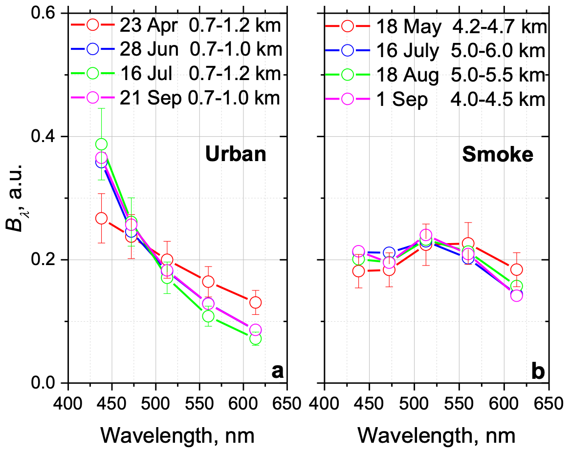
Figure 1 Fluorescence spectra for (a) urban aerosol within the PBL and (b) smoke in the middle troposphere observed in 2024. Spectra are normalized to the sum of the fluorescence backscattering coefficients across all five channels.

In Veselovskii et al. (2025a), the reference spectra $B_{\mathit{\lambda }}^{\text{Uref}}$ and $B_{\mathit{\lambda }}^{\text{Sref}}$ were defined as averages over all 2023 observations. Given the high variability in fluorescence spectra, at present study for each analyzed episode, we selected spatiotemporal intervals expected to represent pure smoke or urban aerosol. When such an interval was unavailable for a given episode, we used appropriate spectra from temporally proximate measurements.

To calculate particle volume concentration from the retrieved backscattering coefficients, we use extinction-to-volume conversion factors at 355 nm specific to urban aerosol, $C_{\mathrm{355}}^{\mathrm{U}}$, and smoke, $C_{\mathrm{355}}^{\mathrm{S}}$. This requires first converting the backscattering coefficients to extinction coefficients:

$$\begin{array}{}\text{(3)}& {\mathit{\alpha }}_{\mathrm{355}}^{\mathrm{U}}={\mathit{\beta }}_{\mathrm{355}}^{\mathrm{U}}\times S_{\mathrm{355}}^{\mathrm{U}}\text{and}{\mathit{\alpha }}_{\mathrm{355}}^{\mathrm{S}}={\mathit{\beta }}_{\mathrm{355}}^{\mathrm{S}}\times S_{\mathrm{355}}^{\mathrm{S}}\end{array}$$

where $S_{\mathrm{355}}^{\mathrm{U}}$ and $S_{\mathrm{355}}^{\mathrm{S}}$ are the corresponding lidar ratios at 355 nm wavelength. The volume concentration for smoke is then:

$$\begin{array}{}\text{(4)}& V_{\mathrm{S}}=C_{\mathrm{355}}^{\mathrm{S}}\times {\mathit{\alpha }}_{\mathrm{355}}^{\mathrm{S}}\end{array}$$

and the mass concentration is given by:

$$\begin{array}{}\text{(5)}& \begin{array}{rl}{M}_{\mathrm{s}}& ={\mathit{\rho }}_{\mathrm{S}}{V}_{\mathrm{S}}={\mathit{\rho }}_{\mathrm{S}}{C}_{\mathrm{355}}^{\mathrm{S}}{\mathit{\alpha }}_{\mathrm{355}}^{\mathrm{S}}={\mathit{\rho }}_{\mathrm{S}}{C}_{\mathrm{355}}^{\mathrm{S}}{S}_{\mathrm{355}}^{\mathrm{S}}{\mathit{\beta }}_{\mathrm{355}}^{\mathrm{S}}\\ & ={\mathit{\rho }}_{\mathrm{S}}{C}_{\mathrm{355}}^{\mathrm{S}}{S}_{\mathrm{355}}^{\mathrm{S}}{\displaystyle \frac{B_{\mathit{\lambda }}^{\mathrm{S}}}{G_{\mathit{\lambda }}^{\mathrm{S}}}}=K_{\mathit{\lambda }}^{\mathrm{S}}{B}_{\mathit{\lambda }}^{\mathrm{S}}\end{array}\end{array}$$

where ρ_S is the smoke density. Thus, factor $K_{\mathit{\lambda }}^{\mathrm{S}}$ relates the fluorescence backscattering to the smoke mass concentration. The mass concentration of urban aerosol is calculated analogously using its respective density ρ_U, conversion factor $C_{\mathrm{355}}^{\mathrm{U}}$ and lidar ratio $S_{\mathrm{355}}^{\mathrm{U}}$. Based on values reported by Li et al. (2016) and Ansmann et al. (2021), the smoke particle density typically falls within the range of 1.0–1.3 g cm⁻³. In this study we use the mean value ρ_S=1.15 g cm⁻³.

The extinction-to-volume conversion factor at 532 nm for aged smoke, $C_{\mathrm{532}}^{\mathrm{S}}$ has been derived by Ansmann et al. (2021) from AERONET measurements and by Veselovskii et al. (2025b) from multiwavelength Mie–Raman lidar observations. Both methods yielded a value of $C_{\mathrm{532}}^{\mathrm{S}}\approx \mathrm{0.13}$ µm³ cm⁻³ Mm. For the conversion of our 355 nm lidar measurements we adopt the value $C_{\mathrm{355}}^{\mathrm{S}}=\mathrm{0.085}\pm \mathrm{0.015}$ µm³ cm⁻³ Mm, reported by Veselovskii et al. (2025b). For urban aerosol a lidar-derived value of $C_{\mathrm{355}}^{\mathrm{U}}=\mathrm{0.08}\pm \mathrm{0.03}$ µm³ cm⁻³ Mm was obtained for Lille, France (Veselovskii et al., 2025b). However, urban aerosol composition, and thus its conversion factor, can vary significantly by region. For instance, the $C_{\mathrm{532}}^{\mathrm{U}}$ value from Lille is nearly half that reported by Mamouri and Ansmann (2017) for Leipzig. Consequently, applying the Lille-derived $C_{\mathrm{355}}^{\mathrm{U}}$ to the urban aerosol in Moscow could introduce substantial uncertainty. In this study we calculate and report mass concentration only for aged smoke. The overall uncertainty in quantifying smoke mass concentration mixed with urban aerosol depends on the combined uncertainties of the parameters used: the smoke density, the lidar ratio, the fluorescence capacity, and the conversion factor. We estimate the total uncertainty of this procedure to be below 40 %. In contrast, the relative spatiotemporal variations in smoke concentration within a single measurement episode can be derived with significantly lower uncertainty, which we estimate to be below 10 %.

2.3 Sensitivity of fluorescence lidar measurements to presence of smoke

As a first step in the analysis of the measurements, it is important to estimate expected sensitivity of fluorescence lidar to the presence of smoke, within the PBL. For an external mixture of urban and smoke particles the total measured fluorescence backscatter is $B_{\mathit{\lambda }}=B_{\mathit{\lambda }}^{\mathrm{U}}+B_{\mathit{\lambda }}^{\mathrm{S}}$.

As mentioned, for the lidar used, a convenient indicator of smoke intrusion to the PBL is an increase of the spectral ratio $R_{\mathrm{560}/\mathrm{438}}$. Pure urban aerosol is characterized by the spectral ratio $R_{\mathrm{560}/\mathrm{438}}^{\mathrm{U}}$. The intrusion of smoke increases this ratio by factor A, such that $R_{\mathrm{560}/\mathrm{438}}=A{R}_{\mathrm{560}/\mathrm{438}}^{\mathrm{U}}$. Thus, measured spectral ratio is:

$$\begin{array}{}\text{(6)}& \begin{array}{rl}{R}_{\mathrm{560}/\mathrm{438}}& ={\displaystyle \frac{B_{\mathrm{560}}^{\mathrm{U}}+B_{\mathrm{560}}^{\mathrm{S}}}{B_{\mathrm{438}}^{\mathrm{U}}+B_{\mathrm{438}}^{\mathrm{S}}}}\\ & ={\displaystyle \frac{R_{\mathrm{560}/\mathrm{438}}^{\mathrm{U}}{B}_{\mathrm{438}}^{\mathrm{U}}+R_{\mathrm{560}/\mathrm{438}}^{\mathrm{S}}{B}_{\mathrm{438}}^{\mathrm{S}}}{B_{\mathrm{438}}^{\mathrm{U}}+B_{\mathrm{438}}^{\mathrm{S}}}}\end{array}\end{array}$$

And consequently:

$$\begin{array}{}\text{(7)}& B_{\mathrm{438}}^{\mathrm{S}}=B_{\mathrm{438}}^{\mathrm{U}}{\displaystyle \frac{R_{\mathrm{560}/\mathrm{438}}^{\mathrm{U}}(\mathrm{1}-A)}{(A{R}_{\mathrm{560}/\mathrm{438}}^{\mathrm{U}}-R_{\mathrm{560}/\mathrm{438}}^{\mathrm{S}})}}\end{array}$$

Our instrument can reliably detect a 10 % change in the spectral ratio (i.e. A=1.1). Using the characteristic values of $R_{\mathrm{560}/\mathrm{438}}^{\mathrm{U}}=\mathrm{0.5}$, $R_{\mathrm{560}/\mathrm{438}}^{\mathrm{S}}=\mathrm{1.5}$ and a typical urban fluorescence backscatter $B_{\mathrm{438}}^{\mathrm{U}}=\mathrm{2}$ ${\mathrm{Tm}}^{-\mathrm{1}}{\mathrm{sr}}^{-\mathrm{1}}{\mathrm{nm}}^{-\mathrm{1}}$, the Eq. (7) yields a detectable smoke fluorescence backscatter of $B_{\mathrm{438}}^{\mathrm{S}}\approx \mathrm{0.1}$ ${\mathrm{Tm}}^{-\mathrm{1}}{\mathrm{sr}}^{-\mathrm{1}}{\mathrm{nm}}^{-\mathrm{1}}$. The smoke mass concentration corresponding to this fluorescence backscatter can be calculated from Eq. (5) as:

$$\begin{array}{}\text{(8)}& M_{\mathrm{S}}={\displaystyle \frac{B_{\mathrm{438}}^{\mathrm{S}}{\mathit{\rho }}_{\mathrm{S}}{C}_{\mathrm{355}}^{\mathrm{S}}{S}_{\mathrm{355}}^{\mathrm{S}}}{G_{\mathrm{438}}^{\mathrm{S}}}}\end{array}$$

Substituting typical aged smoke properties, such as $S_{\mathrm{355}}^{\mathrm{S}}=\mathrm{40}$ sr (Haarig et al., 2018) and $G_{\mathrm{438}}^{\mathrm{S}}=\mathrm{4}\times {\mathrm{10}}^{-\mathrm{6}}$ nm⁻¹ we obtain a detectable smoke mass concentration M_S≈0.1 µg m⁻³. This is a rough estimation, but it reveals high sensitivity of fluorescence technique, which is a direct result of the pronounced difference between the fluorescence spectra of smoke and urban particles. For more accurate evaluation of smoke concentration, it is necessary to solve the system of Eq. (1), as will be done in the following section.

3 Results of the measurements

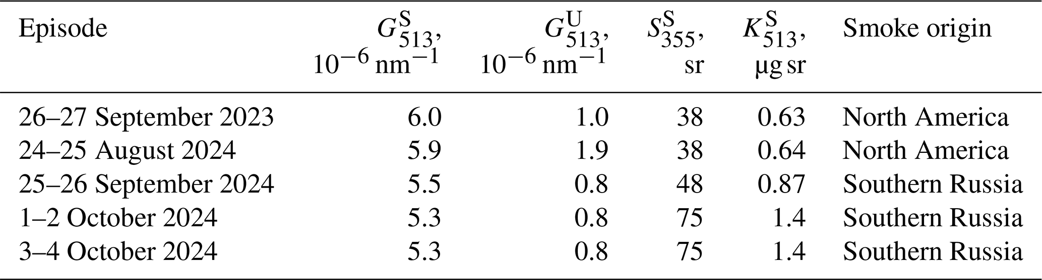
This study analyzes smoke episodes over Moscow in 2023 and 2024 observed with a five-channel fluorescence lidar. Smoke was present during most measurements in the May–October period. In 2024, for instance, we performed 67 measurement sessions from April to October, detecting smoke in 59 episodes. Of these 59 episodes, back-trajectory analysis indicates that the majority were associated with long-range transport from North America, with only 12 originating from fires in southern Russia. In this section, we examine several representative cases, focusing on smoke from both North American wildfires and fires in southern Russia. The values of $G_{\mathrm{513}}^{\mathrm{S}}$, $S_{\mathrm{355}}^{\mathrm{S}}$ and K₅₁₃, used to calculate the smoke mass concentration during the episodes considered in this study, are summarized in Table A1 in the Appendix.

3.1 26–27 September 2023. Long-range transported smoke

On the night of 26–27 September 2023, air masses originating from North America descended from approximately 7000 m to 2000–3500 m height range, as indicated by HYSPLIT backward trajectory analysis (Stein et al., 2015) shown in Fig. 2. This enabled the mixing of transported smoke with urban particles within the PBL. The spatiotemporal distributions of aerosol parameters, such as β₃₅₅, B₅₁₃, G₅₁₃, and $R_{\mathrm{560}/\mathrm{438}}$ are shown in Fig. 3. Two distinct aerosol layers are evident. A lower layer extends from the surface to ∼1250 m altitude. It is characterized by a low fluorescence capacity ($G_{\mathrm{513}}<\mathrm{1.5}\times {\mathrm{10}}^{-\mathrm{6}}$ nm⁻¹) and a low spectral ratio ($R_{\mathrm{560}/\mathrm{438}}<\mathrm{0.7}$), indicating the predominance of urban aerosol. Above 1250 m both G₅₁₃ and $R_{\mathrm{560}/\mathrm{438}}$ increase markedly, with $G_{\mathrm{513}}>\mathrm{4}\times {\mathrm{10}}^{-\mathrm{6}}$ nm⁻¹ and $R_{\mathrm{560}/\mathrm{438}}$ up to 1.5. These values are characteristic of smoke particles. Radiosonde measurements taken at 00:00 UTC on 27 September 2023 reveal a temperature inversion at , confirming this altitude as the PBL top. The smoke layer is thus situated directly atop the PBL. Notably, within the PBL itself, the spectral ratio $R_{\mathrm{560}/\mathrm{438}}$ for the period 17:00–22:00 UTC is higher than that observed during 23:00–00:00 UTC. This suggests that smoke penetrated into the PBL up to approximately 22:00 UTC.

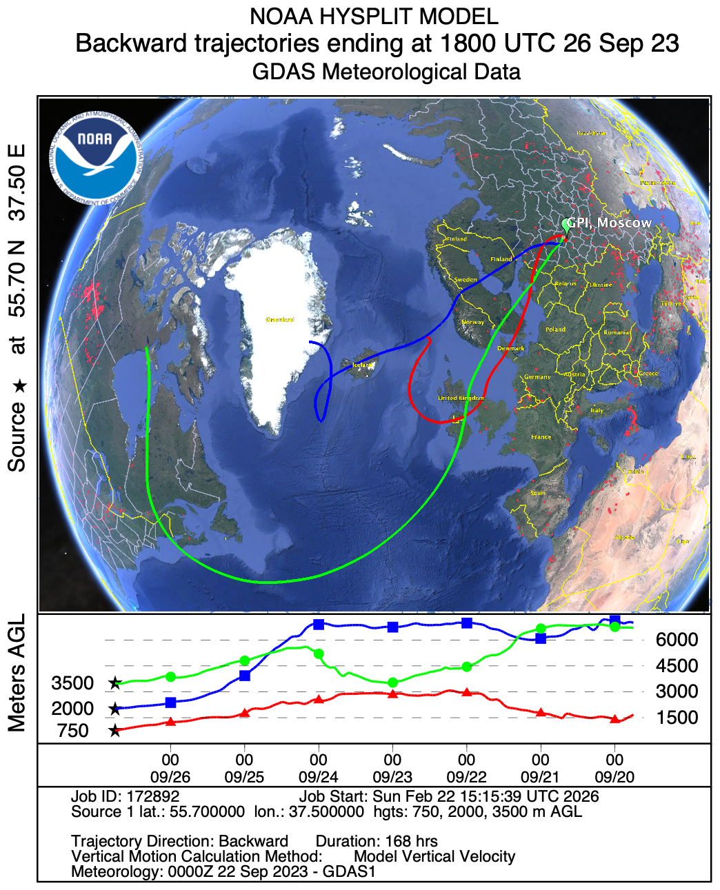
Figure 2 The HYSPLIT six-day backward trajectories for the air mass over Moscow at altitudes 750, 2000, and 3500 m on 26 September 2023 at 18:00 UTC.

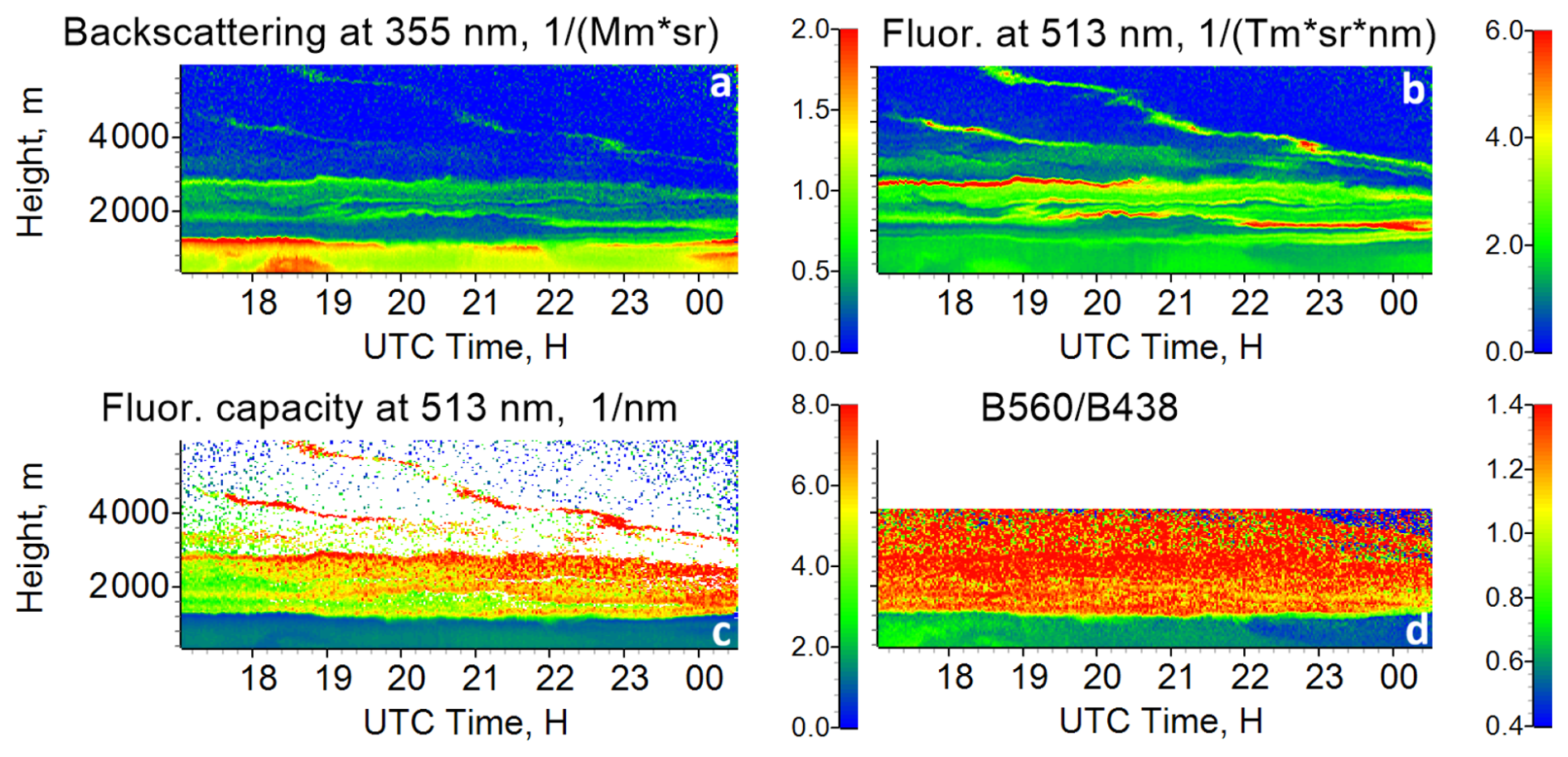
Figure 3 Spatio-temporal distributions of (a) the aerosol backscattering coefficient β₃₅₅ (in ${\mathrm{Mm}}^{-\mathrm{1}}{\mathrm{sr}}^{-\mathrm{1}}$), (b) the fluorescence backscattering coefficient B₅₁₃ (in ${\mathrm{Tm}}^{-\mathrm{1}}{\mathrm{sr}}^{-\mathrm{1}}{\mathrm{nm}}^{-\mathrm{1}}$), (c) the fluorescence capacity G₅₁₃ (in 10⁻⁶ nm⁻¹), and (d) the spectral ratio $B_{\mathrm{560}}/B_{\mathrm{438}}$ during the night of 26–27 September 2023.

To separate the fluorescence backscatter contributions of smoke and urban particles using the method described in Sect. 2, reference spectrum of pure smoke, $B_{\mathit{\lambda }}^{\text{Sref}}$, was derived from the elevated layer at ∼2800 m, where the fluorescence capacity G₅₁₃ exceeded $\mathrm{6}\times {\mathrm{10}}^{-\mathrm{6}}$ nm⁻¹. The pure urban aerosol spectrum, $B_{\mathit{\lambda }}^{\text{Uref}}$, was taken from measurements the previous night (25–26 September), when smoke content within the PBL was below detection limit. The particle parameters used in the analysis of this episode are given in Table A1.

Recall that this method relies on the spectral shape, i.e., the relative fluorescence backscatter across wavelengths. The absolute magnitude is not used directly in the separation algorithm. Formally, the algorithm contains no threshold. However, for low signals, the ratios of fluorescence backscattering in different channels become oscillatory. In data analysis, this manifests as oscillations in the retrieved fluorescence components. Normally, in the lower troposphere, we limit our consideration to values where B₅₁₃>0.5 ${\mathrm{Tm}}^{-\mathrm{1}}{\mathrm{sr}}^{-\mathrm{1}}{\mathrm{nm}}^{-\mathrm{1}}$.

The resulting spatiotemporal distributions of the separated fluorescence backscattering coefficients for urban aerosol, $B_{\mathrm{513}}^{\mathrm{U}}$, and smoke, $B_{\mathrm{513}}^{\mathrm{S}}$, are shown in Fig. 4. Urban aerosol is confined primarily within the PBL. While the main smoke plume resides above the PBL, a significant amount of smoke ($B_{\mathrm{513}}^{\mathrm{S}}$ up to ∼1.0 ${\mathrm{Tm}}^{-\mathrm{1}}{\mathrm{sr}}^{-\mathrm{1}}{\mathrm{nm}}^{-\mathrm{1}}$) is present within the PBL.

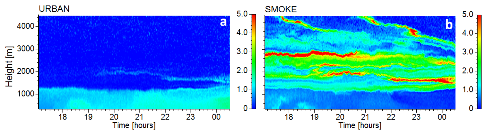
Figure 4 Spatio-temporal distributions of the fluorescence backscattering coefficients (in ${\mathrm{Tm}}^{-\mathrm{1}}{\mathrm{sr}}^{-\mathrm{1}}{\mathrm{nm}}^{-\mathrm{1}}$) attributed to (a) urban, $B_{\mathrm{513}}^{\mathrm{U}}$, and (b) smoke, $B_{\mathrm{513}}^{\mathrm{S}}$, particles on 26–27 September 2023.

Vertical profiles of particle properties averaged from 17:15–23:00 UTC are presented in Fig. 5. Due to incomplete geometrical overlap below ∼1000 m, the lidar ratio within the PBL is not shown. Radiosonde measurements indicate that relative humidity increases with height, reaching 83 % at 1150 m. The observed increase in the aerosol backscattering coefficient β₃₅₅ near the PBL top is likely due to particle hygroscopic growth. Within the PBL, the fluorescence spectral ratio $R_{\mathrm{560}/\mathrm{438}}$ is elevated (∼0.65), indicating a mixture of smoke and urban particles. In contrast, above the PBL, where smoke predominates, this ratio increases to ∼1.5. The spectral shape also differs between layers. Within the PBL, fluorescence decreases monotonically with wavelength, which is characteristic of urban aerosol predominance. Above the PBL, the spectrum exhibits a distinct maximum at 513 nm, a known signature of biomass burning smoke. The potential temperature measured by radiosonde (not shown) is constant up to ∼1200 m, confirming a well-mixed PBL. Therefore, we would expect fluorescence backscatter to be relatively uniform with height within this layer. However, Fig. 5b shows a clear decrease in B₅₁₃ between 500 and 1000 m. This reduction is consistent with fluorescence quenching caused by water uptake at elevated RH, as reported by Veselovskii et al. (2025b).

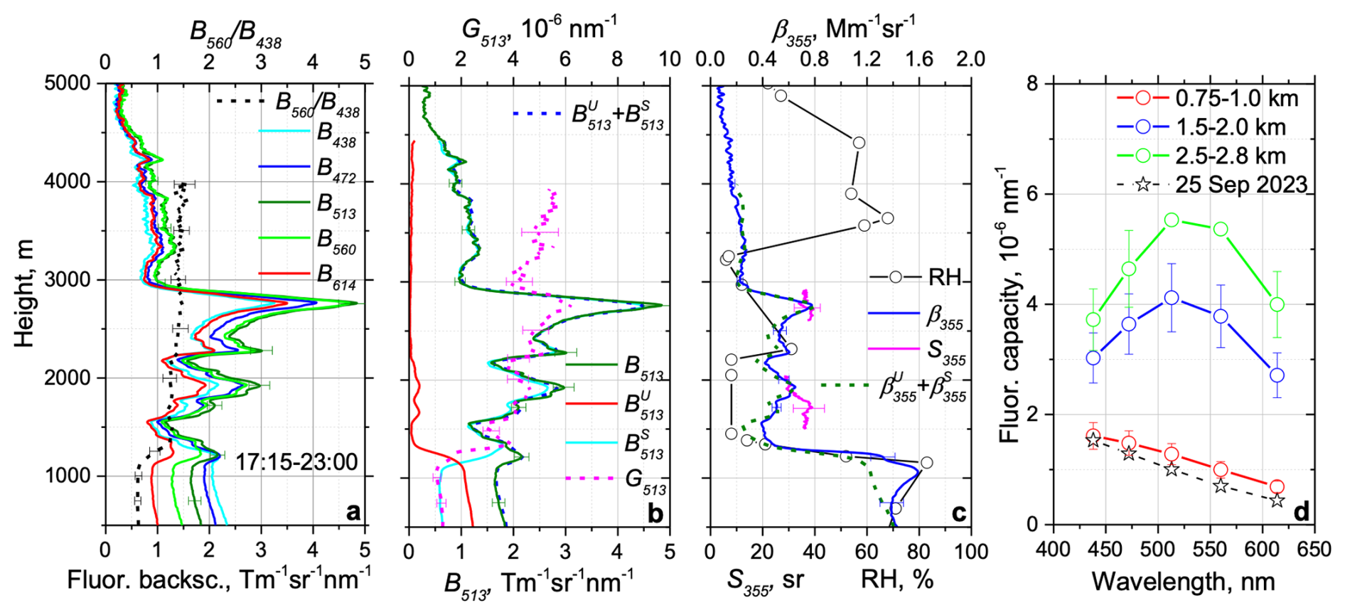
Figure 5 Vertical profiles of particle parameters measured from 17:15–23:00 UTC on 26 September 2023. (a) The fluorescence backscattering coefficients, B_λ, and the spectral ratio $B_{\mathrm{560}}/B_{\mathrm{438}}$. (b) The fluorescence backscattering coefficients attributed to urban, $B_{\mathrm{513}}^{\mathrm{U}}$, and smoke, $B_{\mathrm{513}}^{\mathrm{S}}$, particles, the total measured B₅₁₃, the reconstructed sum $B_{\mathrm{513}}^{\mathrm{U}}+B_{\mathrm{513}}^{\mathrm{S}}$, and the fluorescence capacity, G₅₁₃. (c) The aerosol backscattering coefficient β₃₅₅, the lidar ratio, S₃₅₅, and the reconstructed sum of backscattering coefficients, ${\mathit{\beta }}_{\mathrm{355}}^{\mathrm{U}}+{\mathit{\beta }}_{\mathrm{355}}^{\mathrm{S}}$, attributed to urban and smoke particles. Open symbols show the radiosonde-measured relative humidity, RH. (d) Spectral dependence of fluorescence capacity for different height ranges. The spectrum from 25 September 2023 (0.75–1.0 km), when smoke was absent in the PBL, is shown with stars for reference.

The vertical profiles of the retrieved fluorescence backscattering coefficients $B_{\mathrm{513}}^{\mathrm{U}}$ and $B_{\mathrm{513}}^{\mathrm{S}}$ along with the total fluorescence backscatter B₅₁₃ are shown in Fig. 5b. The reference spectra, used in the retrieval are presented in Fig. 6a. The reference spectrum of smoke is an average taken overnight within the 2600–2800 m height interval. The reference spectrum of urban aerosol was obtained from measurements in the PBL on 25 September 2023, when smoke contamination was minimal.

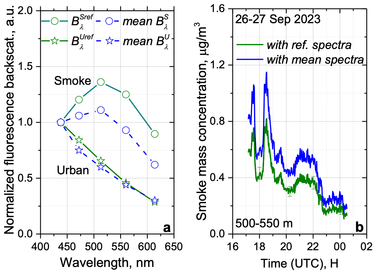
Figure 6 (a) Reference fluorescence backscattering spectra (solid lines) for smoke and urban aerosol used in the retrievals shown in Fig. 5b. Dashed lines represent the 2023 annual mean spectra. All spectra are normalized to their respective values at 438 nm. (b) Temporal evolution of smoke mass concentration within the 500–550 m altitude range, retrieved using the reference spectra and the annual mean spectra from panel (a).

The measured B₅₁₃ is accurately reconstructed by the sum $B_{\mathrm{513}}^{\mathrm{U}}+B_{\mathrm{513}}^{\mathrm{S}}$. To convert $B_{\mathrm{513}}^{\mathrm{U}}$ and $B_{\mathrm{513}}^{\mathrm{S}}$ into corresponding aerosol backscattering coefficients, ${\mathit{\beta }}_{\mathrm{355}}^{\mathrm{U}}$ and ${\mathit{\beta }}_{\mathrm{355}}^{\mathrm{S}}$, accurate values for the fluorescence capacities $G_{\mathrm{513}}^{\mathrm{U}}$ and $G_{\mathrm{513}}^{\mathrm{S}}$ are required. For this case, we used $G_{\mathrm{513}}^{\mathrm{S}}=\mathrm{6.0}\times {\mathrm{10}}^{-\mathrm{6}}$ and $G_{\mathrm{513}}^{\mathrm{U}}=\mathrm{1.0}\times {\mathrm{10}}^{-\mathrm{6}}$ nm⁻¹. The aerosol backscattering coefficient β₃₅₅ is well reconstructed by the sum ${\mathit{\beta }}_{\mathrm{513}}^{\mathrm{U}}+{\mathit{\beta }}_{\mathrm{513}}^{\mathrm{S}}$ within the elevated smoke layers. However, within the PBL, the sum ${\mathit{\beta }}_{\mathrm{513}}^{\mathrm{U}}+{\mathit{\beta }}_{\mathrm{513}}^{\mathrm{S}}$ is systematically less than measured β₃₅₅. This discrepancy is attributed to particle hygroscopic growth occurring at high relative humidity.

The smoke mass concentration, M_S can be derived from Eq. (5). For the elevated smoke layer, the lidar ratio is $S_{\mathrm{355}}^{\mathrm{S}}=\mathrm{38}\pm \mathrm{6}$ sr and $G_{\mathrm{513}}^{\mathrm{S}}=\mathrm{6.0}\times {\mathrm{10}}^{-\mathrm{6}}$ nm⁻¹. For these values, coefficient K₅₁₃ in Eq. (5) is of 0.63 µg sr, meaning that a fluorescence backscatter $B_{\mathrm{513}}^{\mathrm{S}}=\mathrm{1.0}$ ${\mathrm{Tm}}^{-\mathrm{1}}{\mathrm{sr}}^{-\mathrm{1}}{\mathrm{nm}}^{-\mathrm{1}}$ corresponds approximately to a smoke mass concentration of M_S≈0.63 µg m⁻³. From spatiotemporal distribution in Fig. 4b we estimate that the smoke mass concentration exceeds 30±12 µg m⁻³ within the main elevated smoke layer. As noted, smoke mass concentrations within the PBL can be underestimated due to fluorescence quenching during hygroscopic growth. Therefore, to analyze relative trends less affected by this bias, Fig. 6b presents the temporal evolution of the mean smoke mass concentration within the 500–550 m altitude range. This layer was selected because the relative humidity remains below 70 % and the total aerosol backscattering β₃₅₅ is accurately reconstructed by the sum ${\mathit{\beta }}_{\mathrm{513}}^{\mathrm{U}}+{\mathit{\beta }}_{\mathrm{513}}^{\mathrm{S}}$. Within this layer, the derived mass concentration decreased from approximately 0.8±0.3 to 0.2±0.08 µg m⁻³ over the course of the night.

As discussed, the retrieved smoke concentration depends on the choice of reference fluorescence spectra. However, because smoke and urban aerosol have fundamentally different spectral shapes, the retrieval is not overly sensitive to minor spectral variations. Figure 6a compares the reference spectra used in our retrieval (solid lines) with the 2023 annual mean spectra (dashed lines). While the urban aerosol spectrum closely matches $B_{\mathit{\lambda }}^{\text{Uref}}$, the annual mean spectrum for smoke deviates noticeably from the reference spectrum $B_{\mathit{\lambda }}^{\text{Sref}}$ used in the retrieval. The impact of this spectral difference on the retrieved smoke mass concentration is shown in Fig. 6b. Using the annual mean spectra increases the derived concentration by approximately 40 %, although the relative temporal trend is mostly preserved. From these results, we conclude that selecting episode-specific reference spectra is essential for accurate concentration estimates. At the same time, it is reasonable to expect that the fluorescence spectra of pure smoke and urban aerosol do not vary significantly within the PBL during a single episode. Consequently, the retrieval method should reliably capture the relative temporal and vertical variations in smoke mass concentration, particularly under conditions where hygroscopic effects are minimal.

3.2 Smoke from regional fires in southern Russia

Between August and October 2024, intensive wildfires in southern Russia generated multiple episodes of smoke transport to Moscow. In this section, we analyze three representative events: 25–26 September, 1–2 October, and 3–4 October. The corresponding five-day HYSPLIT backward trajectories, shown in Fig. 7, confirm that the sampled air masses passed over active fire regions. These cases exemplify distinct scenarios of smoke interaction with the urban environment: (i) a strong smoke plume directly invades the PBL; (ii) relatively weak smoke plumes are observed against a background of urban aerosol; and (iii) a smoke layer rests atop the PBL. For all three episodes, the relative humidity remained below 60 %. These dry conditions minimized the effects of hygroscopic growth and fluorescence quenching, allowing for a more reliable reconstruction of smoke mass concentration.

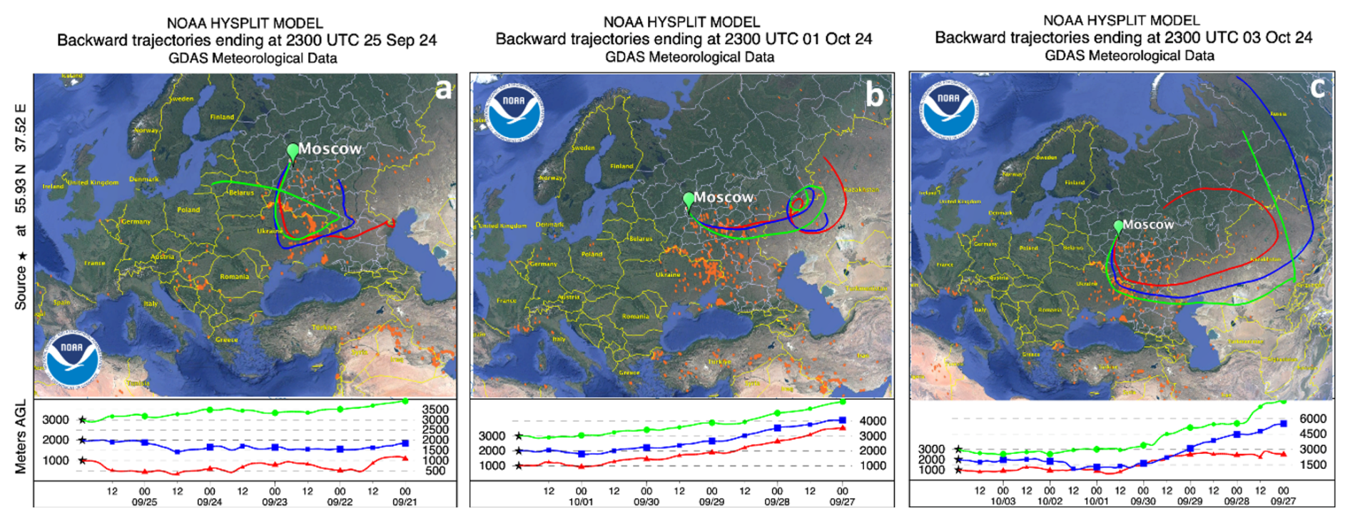
Figure 7 The HYSPLIT five-day backward trajectories for the air mass over Moscow at altitudes 1000, 2000, and 3000 m at 23:00 UTC on (a) 25 September, (b) 1 October and (c) 3 October 2024.

25–26 September 2024

The spatiotemporal distributions of particle parameters (identical to those in Fig. 3) for the night of 25–26 September are presented in Fig. 8. A strong aerosol plume, centered at approximately 1400 m altitude, is observed between 22:00 and 01:00 UTC. Within this plume, the aerosol backscattering coefficient, β₃₅₅, exceeds 10 ${\mathrm{Mm}}^{-\mathrm{1}}{\mathrm{sr}}^{-\mathrm{1}}$. The plume is characterized by an enhanced fluorescence capacity ($G_{\mathrm{513}}>\mathrm{5.0}\times {\mathrm{10}}^{-\mathrm{6}}$ nm⁻¹) and high spectral ratio ($R_{\mathrm{560}/\mathrm{438}}>\mathrm{1.7}$). Figure 7a indicates that the air mass associated with this plume was transported at low altitudes over fire regions near the Black Sea.

Figure 8 Similar to Fig. 3, but for the night of 25–26 September 2024.

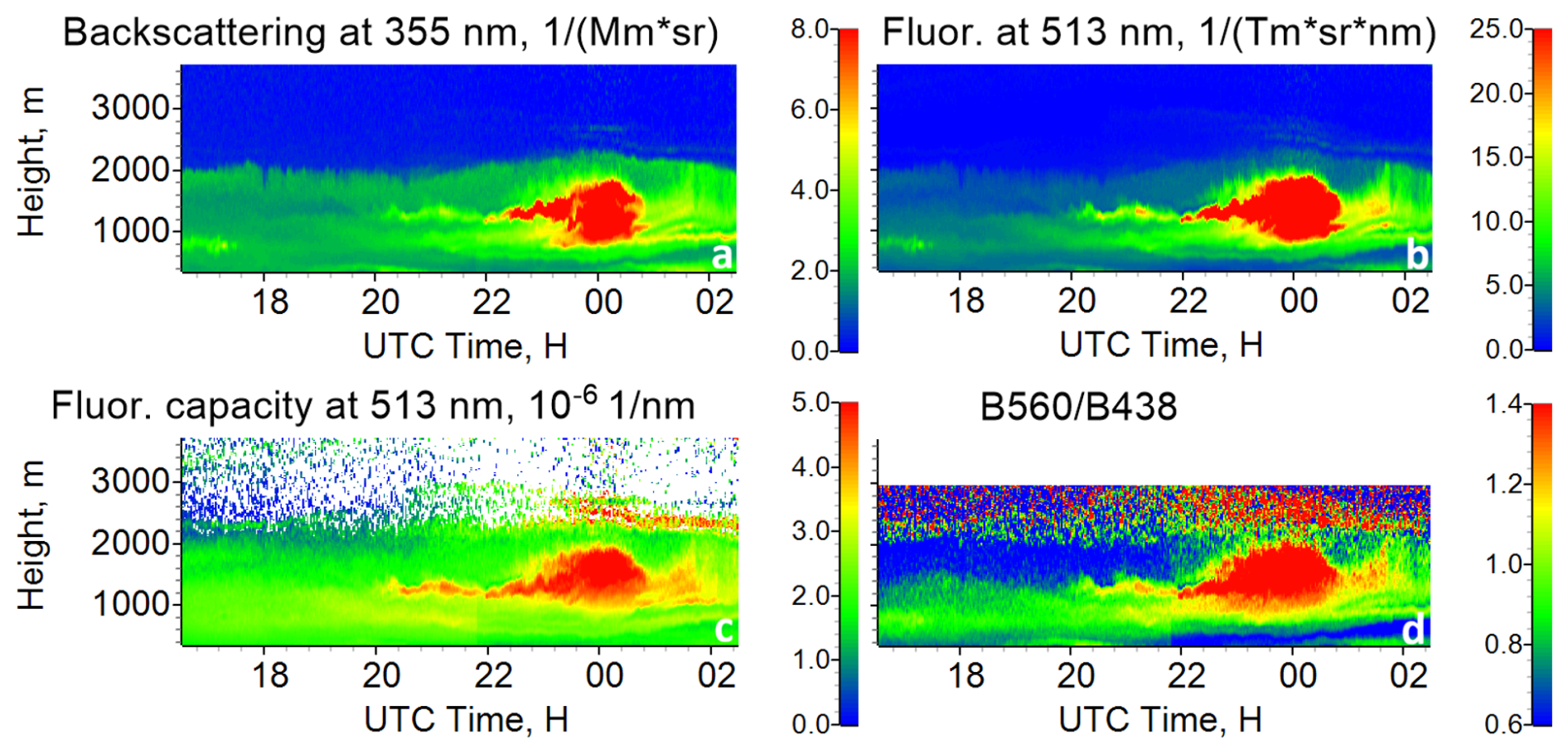
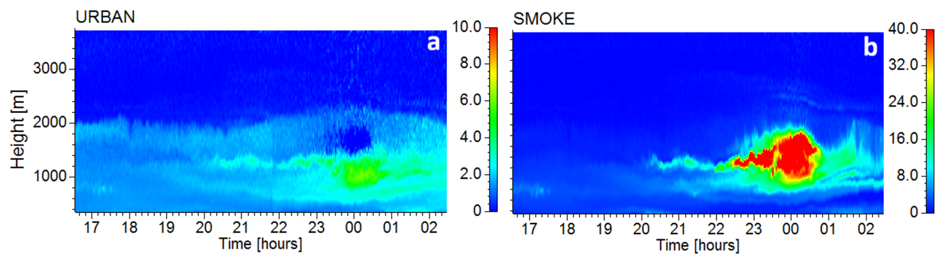
For the separation $B_{\mathrm{513}}^{\mathrm{U}}$ and $B_{\mathrm{513}}^{\mathrm{S}}$, the reference smoke spectrum was obtained near the top of the plume (1600–1800 m altitude), where the fluorescence capacity G₅₁₃ was the highest. The reference urban aerosol spectrum was derived from measurements on 24 August 2024 within the 750–1000 m interval (as will be shown in Fig. 21d), with no smoke in the PBL. The values of $G_{\mathrm{513}}^{\mathrm{U}}=\mathrm{0.8}\times {\mathrm{10}}^{-\mathrm{6}}$ and $G_{\mathrm{513}}^{\mathrm{S}}=\mathrm{5.5}\times {\mathrm{10}}^{-\mathrm{6}}$ nm⁻¹ were used for analysis. The separated fluorescence backscattering coefficients are shown in Fig. 9. The aerosol plume is dominated by smoke, though a moderate increase in urban aerosol concentration within the plume is also observed ($B_{\mathrm{513}}^{\mathrm{U}}$ up to 5 ${\mathrm{Tm}}^{-\mathrm{1}}{\mathrm{sr}}^{-\mathrm{1}}{\mathrm{nm}}^{-\mathrm{1}}$). Outside of plume (17:00–19:00 UTC) the fluorescence backscatter of urban aerosol and smoke is relatively weak ($B_{\mathrm{513}}^{\mathrm{U}}<\mathrm{2}$ and $B_{\mathrm{513}}^{\mathrm{S}}<\mathrm{5}$ ${\mathrm{Tm}}^{-\mathrm{1}}{\mathrm{sr}}^{-\mathrm{1}}{\mathrm{nm}}^{-\mathrm{1}}$).

Figure 9 Similar to Fig. 4, but for the night of 25–26 September 2024.

Vertical profiles of particle parameters within the plume are shown in Fig. 10. The spectral ratio $R_{\mathrm{560}/\mathrm{438}}$ and the fluorescence capacity G₅₁₃ increase with altitude, reaching peak values of approximately 1.75 and $\mathrm{5.5}\times {\mathrm{10}}^{-\mathrm{6}}$ nm⁻¹ respectively, near the plume top (∼1750 m). The lidar ratio also increases slightly from 45 to 48 sr. This vertical gradient likely results from the mixing of the smoke with local background pollution during transport. Additionally, atmospheric aging processes, which can alter particle composition during transport, may further contribute to the observed gradient. The measured B₅₁₃ and β₃₅₅ are well reconstructed by the sums $B_{\mathrm{513}}^{\mathrm{U}}+B_{\mathrm{513}}^{\mathrm{S}}$ and ${\mathit{\beta }}_{\mathrm{513}}^{\mathrm{U}}+{\mathit{\beta }}_{\mathrm{513}}^{\mathrm{S}}$ respectively. Using the G₅₁₃ and S₃₅₅ values from 1700 m we calculate that $K_{\mathrm{513}}^{\mathrm{S}}=\mathrm{0.87}$ µg sr. As follows from Fig. 10b, the maximum smoke mass concentration within the plume is approximately 50±20 µg m⁻³.

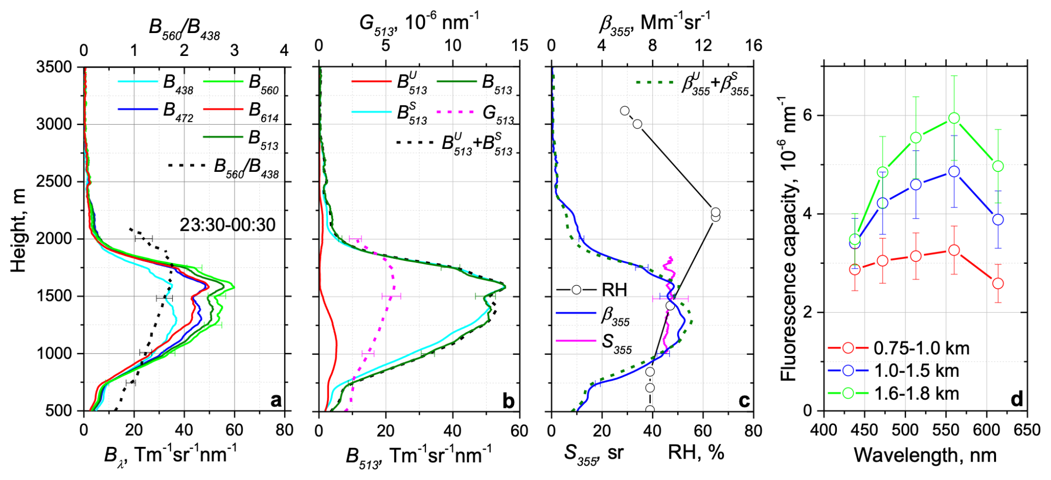
Figure 10 Similar to Fig. 5, but for 25–26 September 2024 for the period 23:30–00:30 UTC. RH profile was obtained from the Global Data Assimilation System (GDAS).

1–2 October 2024

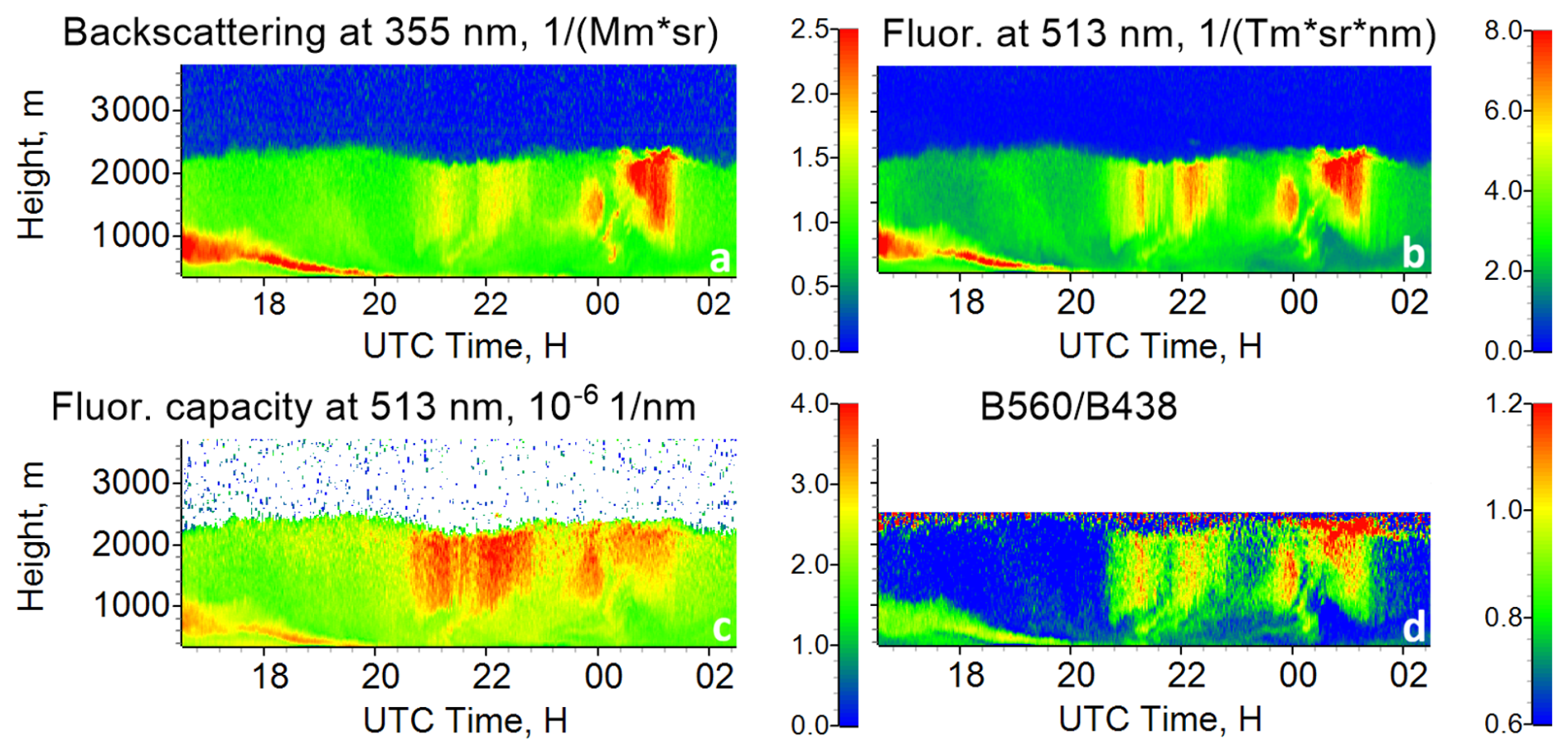
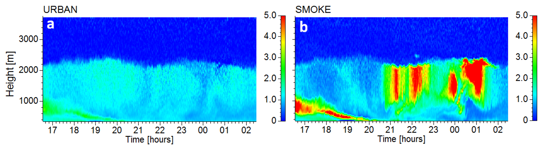
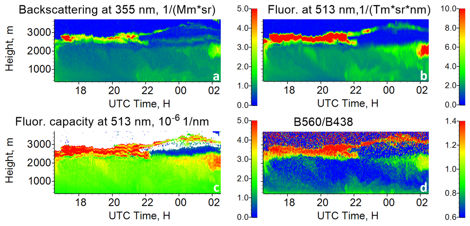
On the night of 1–2 October several intense aerosol plumes were observed within 1000–2000 m altitude range. The air mass trajectory (Fig. 7b) did not intersect the main fire zone but instead skirted its northern periphery. Figure 11 presents the spatiotemporal distributions of the particle parameters (the same as in Fig. 4). Within the plumes the fluorescence capacity G₅₁₃ and the spectral ratio $R_{\mathrm{560}/\mathrm{438}}$ increase to approximately $\mathrm{3}\times {\mathrm{10}}^{-\mathrm{6}}$ nm⁻¹ and 1.2 respectively, which are the values characteristic of smoke. However, these values are lower than in the previous episode, as background urban aerosol contributes significantly to the total fluorescence backscatter in this case.

Figure 11 Similar to Fig. 3, but for the night of 1–2 October 2024.

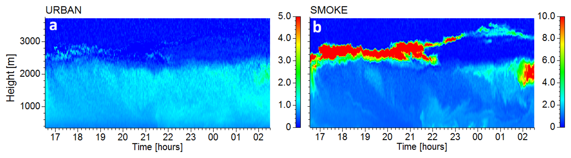
Urban aerosol and smoke were mixed throughout the PBL. To separate their contributions, we used the reference spectrum for urban aerosol measured on 24 August 2024, and the reference spectrum for smoke obtained on 3 October 2024, as detailed in the following section. The results of separation $B_{\mathrm{513}}^{\mathrm{U}}$ and $B_{\mathrm{513}}^{\mathrm{S}}$ are shown in Fig. 12. The distribution of background urban aerosol is relatively uniform, confirming that the observed aerosol plumes consist predominantly of smoke.

Figure 12 Similar to Fig. 4, but for the night of 1–2 October 2024.

Vertical profiles of particle parameters, averaged over the period 00:15–01:15 UTC and encompassing a strong smoke plume, are displayed in Fig. 13. Both the fluorescence capacity G₅₁₃ and the spectral ratio $R_{\mathrm{560}/\mathrm{438}}$, increase with altitude, reaching maximum values of $\mathrm{3.2}\times {\mathrm{10}}^{-\mathrm{6}}$ nm⁻¹ and 1.3 respectively, near the top of the plume. The lidar ratio also increases with height, rising from 50±8 to 60±9 sr. For reference, the lidar ratio for pure smoke measured on 3 October 2024 is 75±10 sr. The observed increase of S₃₅₅ with height is thus consistent with an increasing proportion of smoke in the aerosol mixture. The fluorescence capacity spectra in Fig. 13d differ from those presented for 26 September 2024 (Fig. 10). Specifically, the enhancement in G₅₁₃ and G₅₆₀ near the plume top is less pronounced, which can again be attributed to a greater degree of mixing between smoke and background urban aerosol.

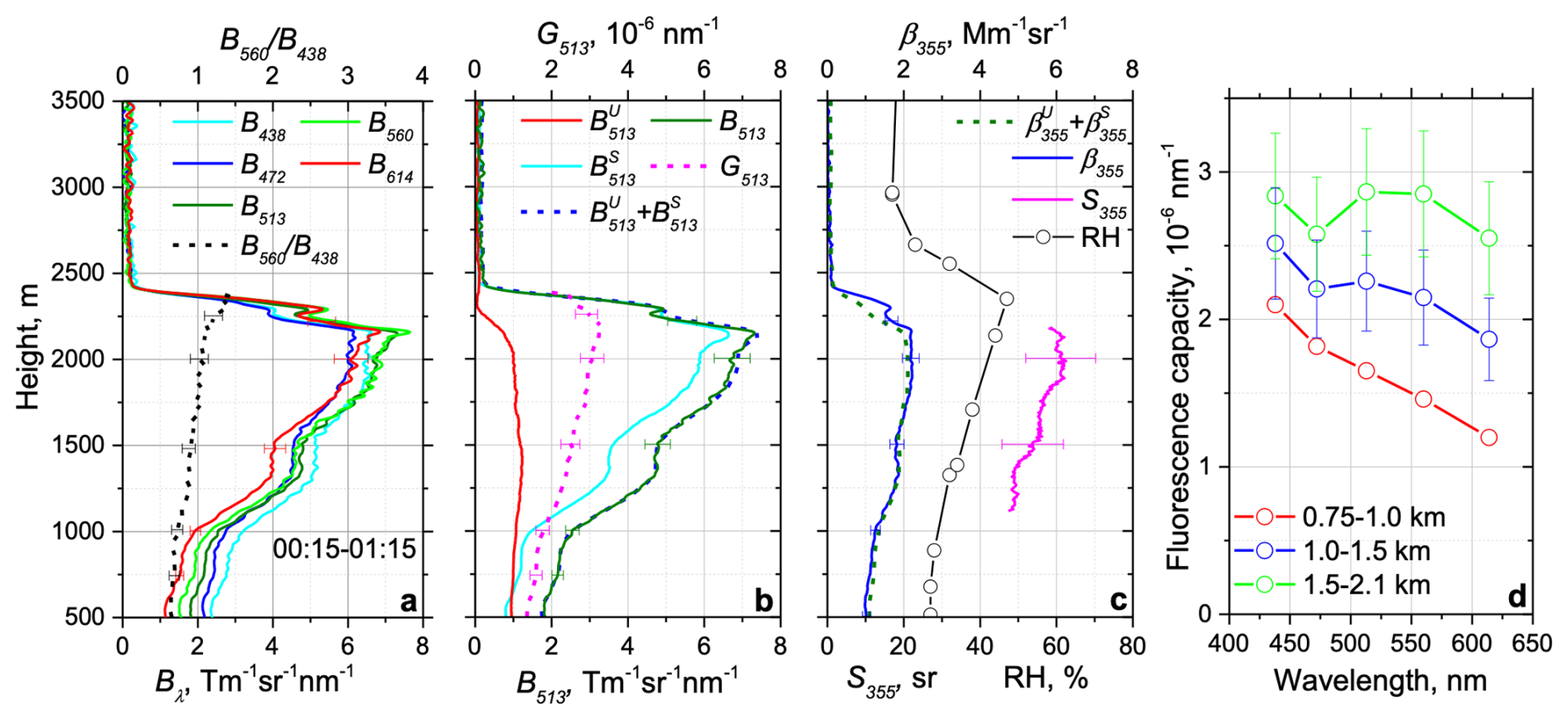
Figure 13 Similar to Fig. 5, but for 2 October 2024 for the period 00:15–01:15 UTC. RH profile was obtained from the GDAS.

For calculation the aerosol backscattering coefficients, we used $G_{\mathrm{513}}^{\mathrm{U}}=\mathrm{0.8}\times {\mathrm{10}}^{-\mathrm{6}}$ nm⁻¹ (from 24 August 2024) and $G_{\mathrm{513}}^{\mathrm{S}}=\mathrm{5.3}\times {\mathrm{10}}^{-\mathrm{6}}$ nm⁻¹ (from 3 October 2024). As shown in Fig. 13c, the measured β₃₅₅ is accurately reconstructed by the sum ${\mathit{\beta }}_{\mathrm{513}}^{\mathrm{U}}+{\mathit{\beta }}_{\mathrm{513}}^{\mathrm{S}}$, corroborating the assumption, that fluorescence capacity of smoke and urban particles remained constant with altitude. Using Eq. (5) with S₃₅₅=75 sr we find that $K_{\mathrm{513}}^{\mathrm{S}}\approx \mathrm{1.4}$ µg sr. Consequently, the maximum smoke mass concentration within the plume is approximately 9.0±3.6 µg m⁻³.

3–4 October 2024

On 3–4 October air mass passed again over region of intense fires (Fig. 7c). As shown in Fig. 14, a smoke layer with high fluorescence capacity ($G_{\mathrm{513}}^{\mathrm{S}}>\mathrm{5}\times {\mathrm{10}}^{-\mathrm{6}}$ nm⁻¹) and a high spectral ratio ($R_{\mathrm{560}/\mathrm{438}}>\mathrm{1.4}$) is located at the top of the PBL between 17:00 and 22:00 UTC. To separate the fluorescence backscattering contributions of smoke and urban aerosol, the smoke reference spectrum was obtained from the 2600–2800 m altitude range, while the urban aerosol reference spectrum was again taken from measurements on 24 August 2024. The resulting spatiotemporal distribution of background urban aerosol, shown in Fig. 15, is relatively uniform, with $B_{\mathrm{513}}^{\mathrm{U}}<\mathrm{1.5}$ ${\mathrm{Tm}}^{-\mathrm{1}}{\mathrm{sr}}^{-\mathrm{1}}{\mathrm{nm}}^{-\mathrm{1}}$. In contrast, the smoke layer atop the PBL exhibited strong fluorescence backscatter $B_{\mathrm{513}}^{\mathrm{S}}>\mathrm{18}$ ${\mathrm{Tm}}^{-\mathrm{1}}{\mathrm{sr}}^{-\mathrm{1}}{\mathrm{nm}}^{-\mathrm{1}}$, while within the PBL $B_{\mathrm{513}}^{\mathrm{S}}$ remained low (below 2 ${\mathrm{Tm}}^{-\mathrm{1}}{\mathrm{sr}}^{-\mathrm{1}}{\mathrm{nm}}^{-\mathrm{1}}$). Thus, smoke was primarily localized above, rather than within, the PBL.

Figure 14 Similar to Fig. 3, but for the night of 3–4 October, 2024.

Figure 15 Similar to Fig. 4, but for the night of 3–4 October, 2024.

Vertical profiles of particle parameters averaged over the 16:50–22:00 UTC period are shown in Fig. 16. A smoke layer atop the PBL is centered at approximately 2700 m, with a peak aerosol backscattering coefficient β₃₅₅ of 3.5 ${\mathrm{Mm}}^{-\mathrm{1}}{\mathrm{sr}}^{-\mathrm{1}}$. Within this layer both the spectral ratio $R_{\mathrm{560}/\mathrm{438}}$ and the fluorescence capacity G₅₁₃ increase sharply to values of 1.4 and $\mathrm{5.3}\times {\mathrm{10}}^{-\mathrm{6}}$ nm⁻¹ respectively. Below 2250 m the lidar ratio is 45±7 sr, but within the smoke layer S₃₅₅ increases to 75±10 sr, a value typical for fresh smoke (Haarig et al., 2016).

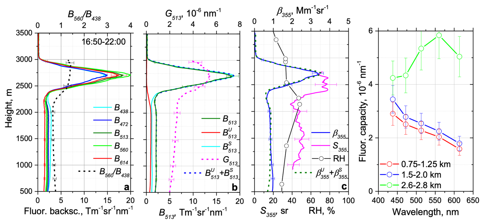
Figure 16 Similar to Fig. 5, but for 3 October 2024 for the period 16:50–22:00 UTC. RH profile was obtained from GDAS.

For the calculation of aerosol backscattering coefficients ${\mathit{\beta }}_{\mathrm{513}}^{\mathrm{U}}$ and ${\mathit{\beta }}_{\mathrm{513}}^{\mathrm{S}}$ we used fluorescence capacities $G_{\mathrm{513}}^{\mathrm{U}}=\mathrm{0.8}\times {\mathrm{10}}^{-\mathrm{6}}$ and $G_{\mathrm{513}}^{\mathrm{S}}=\mathrm{5.3}\times {\mathrm{10}}^{-\mathrm{6}}$ nm⁻¹. The sum $B_{\mathrm{513}}^{\mathrm{U}}+B_{\mathrm{513}}^{\mathrm{S}}$ accurate reconstructs the measured fluorescence profile B₅₁₃ at all altitudes. However, for the aerosol backscattering coefficient, the sum ${\mathit{\beta }}_{\mathrm{513}}^{\mathrm{U}}+{\mathit{\beta }}_{\mathrm{513}}^{\mathrm{S}}$ falls below the measured β₃₅₅ at altitudes below 1000 m. This discrepancy may be due to a change in the composition of urban aerosol at these lower altitudes. The factor $K_{\mathrm{513}}^{\mathrm{S}}$ from Eq. (5) is approximately 1.4 µg sr, therefore, the maximum smoke mass concentration within the smoke layer is 23±9 µg m⁻³, while within the PBL this value is below 2±0.8 µg m⁻³.

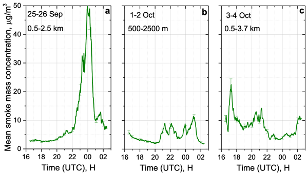
The fluorescence measurements allow to evaluate the temporal evolution of the smoke mass concentration mixed with the background urban aerosol. Figure 17 shows the mean smoke mass concentration for the three episodes discussed in this section. Values are averaged within the altitude intervals indicated on the plots. On 25–26 September, the concentration was highest, reaching ∼50 µg m⁻³. On 1–2 October, concentrations were lower, peaking near 10 µg m⁻³. On 3–4 October, the mean concentration was enhanced at the beginning of the measurements (M_S>20 µg m⁻³) due to the presence of the elevated smoke layer and then it decreased to ∼4 µg m⁻³. The results presented in this section demonstrate that smoke from regional fires leads to significantly higher concentrations within the PBL compared to long-range transported North American smoke.

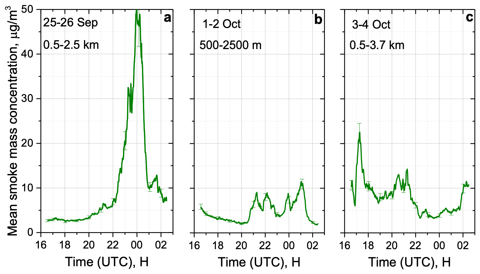
Figure 17 Temporal evolution of the mean smoke mass concentration for the periods (a) 25–26 September, (b) 1–2 October and (c) 3–4 October 2024. Data are averaged over the height intervals of 0.5–2.5, 0.5–2.5 and 0.75–3.7 km, respectively.

3.3 Extreme pollution event on 24–25 August 2024

While the dominant aerosol layers observed in our 2024 measurements originated from fires, and the technique described in this paper reliably separates smoke from background urban aerosol, we also identified episodes involving transported layers with high optical depth (OD) that were attributed to anthropogenic pollution. This section presents one such episode from 24–25 August 2024.

HYSPLIT seven-day backward trajectories for air masses over Moscow at 1000, 2000, and 4300 m are shown in Fig. 18. The episode featured a complex multi-layered aerosol structure. Relative humidity from the Global Data Assimilation System (GDAS) remained below 60 % thus, minimizing interference of particle hygroscopic growth on data analysis. The spatiotemporal distributions of particle parameters are presented in Fig. 19. At the start of the measurements a layer at ∼5000 m descended overnight to ∼4000 m. This layer exhibited a high fluorescence capacity $G_{\mathrm{513}}>\mathrm{5}\times {\mathrm{10}}^{-\mathrm{6}}$ nm⁻¹ and spectral ratio $R_{\mathrm{560}/\mathrm{438}}>\mathrm{1.0}$, identifying it as smoke from Canadian wildfires, consistent with the backward trajectories in Fig. 18.

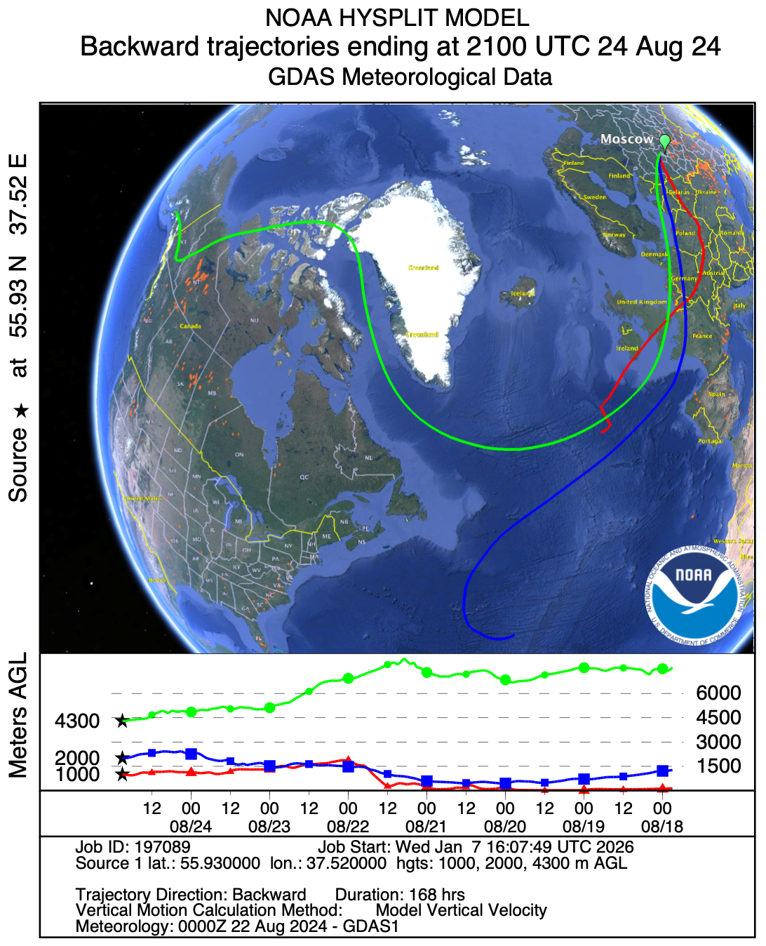
Figure 18 The HYSPLIT seven-day backward trajectories for the air mass over Moscow at altitudes 1000, 2000, and 4300 m on 24 August 2024 at 21:00 UTC.

Figure 19 Similar to Fig. 3, but for the night of 24–25 August 2024.

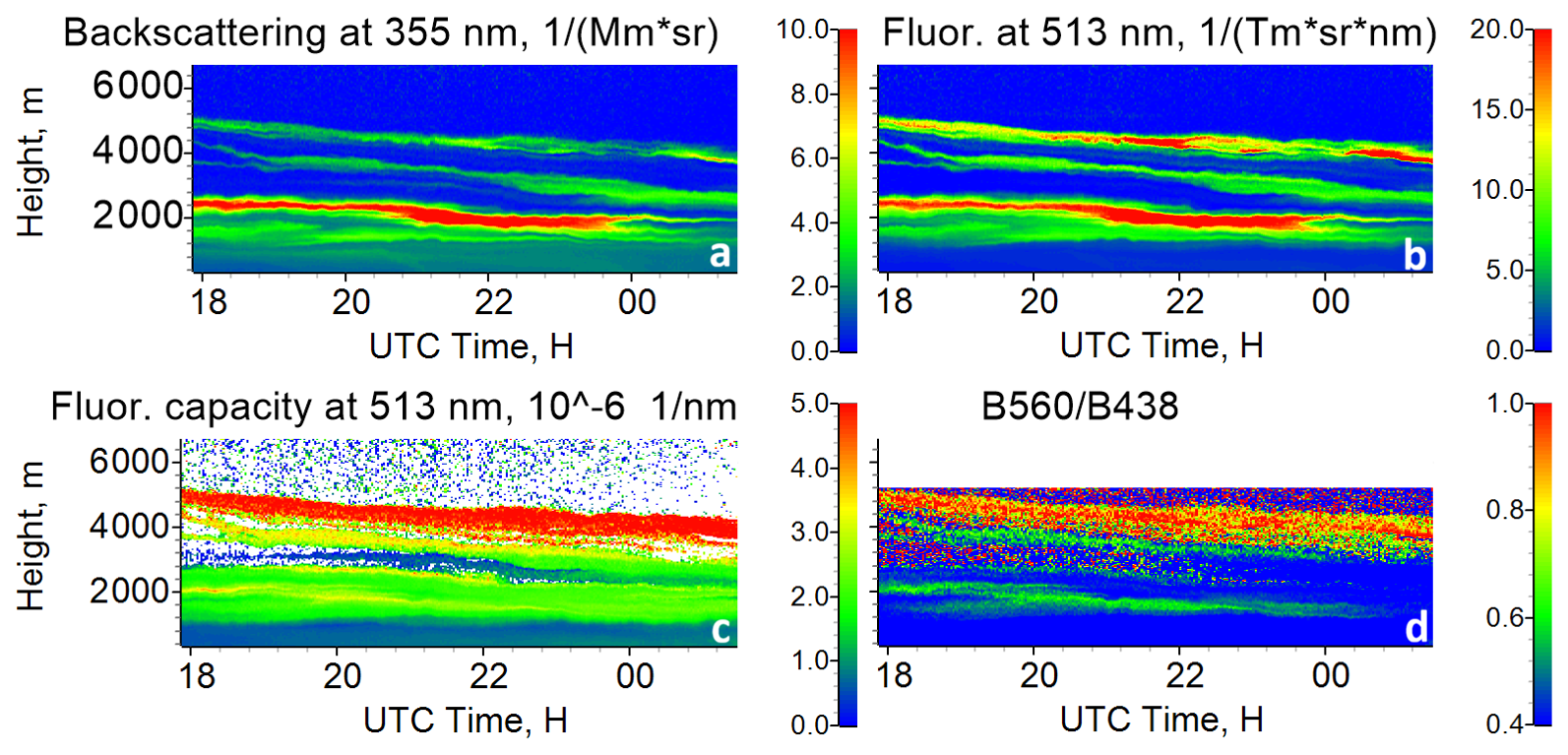
A second strong layer with the aerosol backscattering coefficient β₃₅₅>10 ${\mathrm{Mm}}^{-\mathrm{1}}{\mathrm{sr}}^{-\mathrm{1}}$ was observed initially at ∼2500 m and descended to ∼2000 m. Its fluorescence characteristics, $G_{\mathrm{513}}\sim \mathrm{2}\times {\mathrm{10}}^{-\mathrm{6}}$ nm⁻¹ and $R_{\mathrm{560}/\mathrm{438}}$ ∼0.5, are indicative of urban/industrial particles. The corresponding backward trajectories show transport at low altitudes across Europe, likely passing over a strong pollution source, though we cannot presently identify its exact origin. To separate the contributions of urban aerosol and smoke we used the reference fluorescence spectra, measured within 750–1000 m range for urban particles, within 4100–4400 m for smoke and averaged from 21:00 to 24:00 UTC. The results of this separation are shown in Fig. 20. The smoke is predominantly contained in the upper layer, while aerosol below 4000 m consists mainly of urban particles.

Figure 20 Similar to Fig. 4, but for the night of 24–25 August 2024.

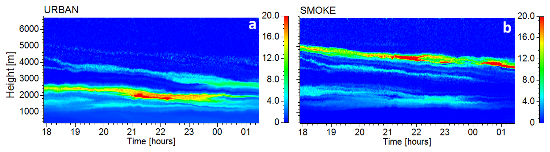
Vertical profiles of particle parameters are shown in Fig. 21. The aerosol backscattering coefficient in the layer centered at 2000 m peaks near 10 ${\mathrm{Mm}}^{-\mathrm{1}}{\mathrm{sr}}^{-\mathrm{1}}$. The lidar ratio in this layer is $S_{\mathrm{355}}=\mathrm{30}\pm \mathrm{5}$ sr and it is even lower (S₃₅₅∼25 ±4 sr) between 2750 and 3750 m, values that are too low for aged smoke. The characteristic lidar ratio for long-range transported Canadian smoke $S_{\mathrm{355}}=\mathrm{38}\pm \mathrm{6}$ sr, typical for long transported Canadian smoke, is observed only in the layer near 4300 m.

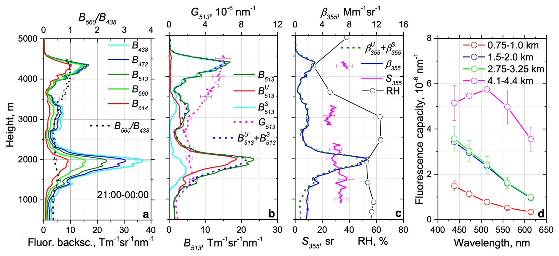
Figure 21 Similar to Fig. 5, but for 24 August 2024 for the period 21:00–00:00 UTC. RH profile was obtained from the GDAS.

The spectrum of fluorescence capacity within the 750–1000 m range (Fig. 21d) and the value $G_{\mathrm{513}}=\mathrm{0.8}\times {\mathrm{10}}^{-\mathrm{6}}$ nm⁻¹ are typical for background urban aerosol. In contrast, within the layers at 2000 and 3000 m, G₅₁₃ increases to $\mathrm{2.3}\times {\mathrm{10}}^{-\mathrm{6}}$ nm⁻¹, while the spectral shape remains similar ($R_{\mathrm{560}/\mathrm{438}}\sim \mathrm{0.5}$). This indicates that the urban aerosol above 1400 m has a different composition. A likely explanation is an elevated proportion of organic components (relative to inorganic species like sulfates and nitrates) in the transported pollution layer.

Results of separation the fluorescence backscatters $B_{\mathrm{513}}^{\mathrm{U}}$ and $B_{\mathrm{513}}^{\mathrm{S}}$ are shown in Fig. 21b. The sum $B_{\mathrm{513}}^{\mathrm{U}}+B_{\mathrm{513}}^{\mathrm{S}}$ accurately reconstructs the measured total fluorescence profile B₅₁₃ at all altitudes. Urban aerosol predominates in the layers at 2000 and 3000 m, though a minor smoke component is also present. To calculate the aerosol backscattering coefficients ${\mathit{\beta }}_{\mathrm{513}}^{\mathrm{U}}$ and ${\mathit{\beta }}_{\mathrm{513}}^{\mathrm{S}}$ via Eq. (2), we used fluorescence capacities $G_{\mathrm{513}}^{\mathrm{U}}=\mathrm{1.9}\times {\mathrm{10}}^{-\mathrm{6}}$ and $G_{\mathrm{513}}^{\mathrm{S}}=\mathrm{5.8}\times {\mathrm{10}}^{-\mathrm{6}}$ nm⁻¹. Since the urban aerosol composition differs below 1400 m, $G_{\mathrm{513}}^{\mathrm{U}}$ was taken from the 2600 m altitude, where the smoke contribution was minimal. The sum ${\mathit{\beta }}_{\mathrm{513}}^{\mathrm{U}}+{\mathit{\beta }}_{\mathrm{513}}^{\mathrm{S}}$ reconstructs the measured β₃₅₅ well above 1400 m and strongly underestimates it below that height, due to the difference in urban aerosol properties.

Converting the retrieved smoke fluorescence backscatter to mass concentration, shows that $K_{\mathrm{513}}^{\mathrm{S}}\approx \mathrm{0.64}$ µg sr. Consequently, the smoke mass concentration within the layer at is estimated as 3±1.2 µg m⁻³. This episode demonstrates that transported pollution layers can have a composition distinct from the local background urban aerosol. While the source of the pollution layer remains unidentified, the method provides fluorescent signatures for distinguishing such events.

4 Conclusions

The results presented in this study demonstrate that a lidar equipped with several discrete fluorescence channels enables the retrieval of smoke mass concentration within the PBL, even when smoke is mixed with urban aerosol. The technique exhibits high sensitivity, capable of detecting vertical and temporal variations in M_S with an estimated detection threshold of approximately 0.1 µg m⁻³. Observations over Moscow from 2023 to 2024 reveal that from spring through autumn, smoke was frequently present not only in the free troposphere but also within the PBL, intermixed with background urban aerosol. The episodes considered in this study are representative and were selected to demonstrate different scenarios of smoke and urban aerosol mixing within the PBL. Notably, long-range transported smoke from North American wildfires contributed up to ∼1 µg m⁻³ to the PBL mass concentration in Moscow. Regional wildfires constituted another significant source of smoke. During August–October 2024 we observed 12 episodes where smoke from fires in southern Russia was detected within the Moscow PBL, with mass concentrations reaching up to 50 µg m⁻³.

The use of multi-channel fluorescence lidar thus moves fluorescence lidar beyond qualitative aerosol-classification tool and towards a quantitative methodology capable of monitoring the dynamics of smoke-urban aerosol mixing. However, the accuracy of the quantitative retrieval is influenced by several factors. In particular, the fluorescence quenching by water uptake during hygroscopic growth may require dedicated correction schemes. A further priority for future work is the validation of this retrieval technique through direct comparison with in situ, ground-based aerosol measurements, in order to better quantify the total uncertainty budget and to strengthen the fluorescence-to-mass conversion.

A further practical consideration involves instrumental trade-offs. To measure fluorescence across a wide spectral range, we have chosen a system configuration that excluded simultaneous aerosol measurements at 532 and 1064 nm. The traditional 3β+2α lidar observations (three aerosol backscattering and two extinction coefficients), along with multi-wavelength depolarization measurements, remain a valuable tool for aerosol characterization. Therefore, a compromise for future integrated lidar systems may involve the synergistic use of 2–3 discrete fluorescence channels (within the ∼420–520 nm spectral range) along with Mie–Raman measurements at 532 and 1064 nm wavelengths. At present, such strategy is developed at ATOLL (ATmospheric Observation at LiLLe) instrumentation site at the Laboratoire d'Optique Atmosphérique, University of Lille.

Appendix A

Table A1 summarizes the particles parameters used in the analysis of smoke episodes in this study. The fluorescence capacities $G_{\mathrm{513}}^{\mathrm{S}}$ of long-range transported North American smoke and of regional smoke from southern Russia are similar and vary within the interval (5.3–6.0) $\times {\mathrm{10}}^{-\mathrm{6}}$ nm⁻¹. The lidar ratios of regional smoke in October 2024 were twice as high as those of North American smoke. Consequently, the factors $K_{\mathrm{513}}^{\mathrm{S}}$ for regional smoke are also higher. We should also recall that, when separating the fluorescence contributions of smoke and urban particles, only the normalized reference spectra are used; therefore, the absolute value of $G_{\mathrm{513}}^{\mathrm{U}}$ is not employed in calculating the smoke mass concentration. It is only essential for verifying that the aerosol backscattering coefficient β₃₅₅ is well reconstructed by the sum of corresponding contributions ${\mathit{\beta }}_{\mathrm{513}}^{\mathrm{U}}+{\mathit{\beta }}_{\mathrm{513}}^{\mathrm{S}}$.

Table A1 The particle parameters used for the analysis of smoke episodes in this study.