Cloud height mapping using multi simultaneous sky images from an all-sky camera network

This study presents a refined, automated in near-real time methodology to obtain cloud height maps using a network of 20 all-sky cameras. This low-cost and easily manipulated instruments are distributed in the city of Valladolid, Spain, trying to cover uniformly an estimated area up to 200 km², with the actual spatial coverage depending on cloud height. Camera distances vary from more than 50 km to less than 200 m, in order to have different viewing angles of the clouds above them. All these cameras are geometrically calibrated and maintained within GOA-SCAN (Group of Atmospheric Optics all-Sky CAmeras Network). The methodology utilizes a stereoscopic approach, pairing simultaneous images from all the cameras. Correlation between the image pixels is computed in order to find the same sky point in both images. Then knowing the baseline distance and the orientation of the cameras, the height of every pixel identified as cloudy is computed. This is repeated for all the camera pairs that have a significant overlapping field of view. Filtering criteria are applied to retain only the significant values. With this methodology, cloud base and top heights (CBH and CTH) maps with a 50 m spatial resolution are obtained every five minutes during daytime and every two minutes for nighttime. These maps are compared with the scene classification product from Sentinel-2 satellite images, finding significant agreement. Some discrepancies were found for high transparent clouds and cloud edges. In addition, all CBH and CTH data available during two and a half years are compared against the independent values measured by a ceilometer collocated with one of the cameras. The determination coefficient for the median CBH values within a circular 150 m distance is 0.93. The obtained CTH values tend to overestimate the ceilometer ones and have wider dispersion, with lower determination coefficient of 0.72. Illuminating conditions are crucial for the correct segmentation of cloudy pixels, limiting the performance of the algorithm at nighttime. Overall, the proposed methodology is promising for obtaining cloud spatial masks and cloud height maps, over different cloud types, layering and conditions.

1 Introduction

It is estimated that approximately 67 % of the Earth is continuously covered by clouds (King et al., 2013); therefore they play a key role in Earth's energy budget. Clouds, mainly formed by liquid water and ice crystals, reflect and absorb part of solar and thermal radiation; hence, they regulate the distribution of the radiative energy in the Earth-atmosphere system, modulating big scale atmospheric dynamics but also small scale regional processes (Hartmann, 1993). In recent years, this topic has attracted particular interest due to the considerable uncertainty that remains in cloud–atmosphere feedbacks (IPCC, 2023). Estimations of cloud vertical structure, specifically cloud base height (CBH) and cloud top height (CTH), are essential for studying the radiative effect of clouds, as properties such as radiative forcing or heating rates are highly height dependent (Stephens, 2005). Cloud height estimations serves as well as a fundamental physical constraint for cloud typing (Huertas-Tato et al., 2017).

Cloud height mapping is interesting for all the aforementioned reasons, but it also has other applications. Knowing CBH with spatial resolution can also be very useful for cloud monitoring, as it helps to understand formation and dissipation processes, as well as the evolution of clouds under different regimes (Seiz and Davies, 2006). This is particularly important for climate and weather prediction models. Another application is solar nowcasting, which requires capturing the high spatio-temporal variability of cloudiness to predict the solar energy budget in near-real time (Cirés et al., 2019). Accurate short-term cloudiness forecasting combined with detailed information on the 3D cloud field have been proven essential for the integration of renewable energy into power grids, as it allows for the prediction of irradiance fluctuations and ramp-rate events, thereby facilitating more efficient plant management and grid stability (Gregor et al., 2023; Papachristopoulou et al., 2024; Papadimitriou et al., 2026). These estimations are also crucial for other issues related to visibility, particularly in aviation but also for monitoring local atmospheric conditions that affect road and maritime transport, as well as for civil protection in adverse weather situations (Isaac et al., 2014).

Several remote sensing techniques are currently employed to estimate cloud base height. Ground based ceilometers and lidars offer high temporal resolution as they provide continuous and reliable direct measurements of CBH; however, these instruments are limited to a narrow field of view, generally measuring only at the zenith, lacking spatial resolution (Costa-Surós et al., 2013). Another ground based instrument is the cloud radar, which can retrieve more detailed cloud microphysical properties and reconstruct the cloud field by scanning the sky (Lamer et al., 2014). However, the minimum time required to complete a 360° sweep limits the ability to describe a cloud field in real time (Borque et al., 2014). These systems also involve high operational complexity and cost. On the other hand, satellites provide global coverage and information on cloud masks and CTH, but retrieving CBH requires additional assumptions (Zhang et al., 2025). Although satellite observations have an extensive global coverage, the temporal and spatial resolution of this data is often insufficient for short-term applications or regional studies (Hamann et al., 2014; Noh et al., 2017). Also, satellite based cloud retrievals often face challenges in accurately identifying cloud shadows (Zhai et al., 2018), and in resolving the 3D structure of clouds, which can lead to significant uncertainties (Yu et al., 2024).

In this framework, the use of all-sky cameras has increased as these cost effective instruments are relatively simple and accessible technology, have low maintenance requirements, and ease of deployment compared to active remote sensing instruments such as lidars and cloud radars, while still providing valuable scientific information for monitoring cloud properties such as cloud cover, cloud type or cloud modification factor among others (Calbó and Sabburg, 2008; Li et al., 2022; González-Fernández et al., 2024). In addition, all-sky cameras have a wide field of view, providing sky images with information of the spatial cloud field with high temporal resolution. These characteristics make them particularly attractive for operational applications such as solar nowcasting in urban environments and over distributed solar power plants (Rodríguez-Benítez et al., 2021). While a single all-sky camera can effectively localize the relative position of clouds within an image (Arbizu-Barrena et al., 2015), it lacks the inherent capability of a lidar or ceilometer to measure vertical distance, nor can it provide the absolute geographic coordinates typical of satellite data. However, this limitation can be overcome by multi-camera setups. Using stereoscopic techniques with two or more synchronized devices, it is possible to triangulate the three-dimensional geometry of cloud fields. This approach not only yields cloud height estimations but also determines cloud spatial positioning, providing a complete picture of their extent.

Nguyen and Kleissl (2014) attempted to obtain the CBH from two daytime images taken by a pair of all-sky cameras, located 1230 m apart, using two different methods. Both approaches used a cloud mask filter based on the saturation channel of the RGB images to remove the cloud-free and sun pixels. The first method was bidimensional and used the georeferenced projection of the images at different hypothetical heights. The mean bias error of the overlapping pixels was computed, and the height that minimizes this error was selected as the CBH. This method was proven to produce root mean square errors of less than 400 m when compared with a ceilometer, and the computational time cost was minimal (2 s per image). However, it did not provide information about different cloud layers, as only a single height value was obtained for the entire layer. The second proposed method was based on epipolar geometry and tried to find the cloud pixel seen in one of the images in the projection of the line joining the center of the camera and that pixel to the other camera image. This method provided three-dimensional information about the clouds, but it had some difficulty with the homogeneous central part of the clouds due to spurious pixel correlation. To address this issue, the reversed process of computing the epipolar line in the other camera was attempted. However, this resulted in a high computational cost. As a potential improvement, the authors suggested incorporating the correlation values of neighbour pixels along the epipolar line to refine the matching process and reduce ambiguities.

Beekmans et al. (2016) proposed another approach to the three-dimensional reconstruction of the clouds during daytime also using a pair of all-sky cameras. Provided the calibration parameters of the cameras it is possible to align the images of both cameras with respect to their baseline so that the epipolar lines matches the rows of the images. This improves the computational cost, as it is only necessary to search in the same row for correlation of one pixel. In order to improve the sensitivity, the comparison was not done pixel by pixel but in small blocks that tried to avoid multiple matching and reduce noise problems. The authors pointed out the potential of this method for the study of convective clouds but the limitation of the retrieval to 5–6 km cloud heights due to the short baseline distance between the used cameras (330 m), and suggested the implementation of a third camera in order to make a more robust analysis.

A similar approach was proposed by Crispel and Roberts (2018), using two all-sky cameras situated 150 m apart and aligned in the same horizontal plane. After correcting for fish-eye lens distortion using a laboratory calibration method (Scaramuzza et al., 2006), the two images were matched using differentiated elements in the images, such as borders or textures, via the Scale Invariant Feature Transform (SIFT) algorithm (Lowe, 2004). Using the paired points and epipolar geometry, the essential matrix was computed by the least median of squares method. This matrix contains information about the orientation and relative position of the cameras. It is therefore possible to obtain the rotation and translation matrices that enable the alignment of the two camera images by their rows. Once the images were aligned, a block-matching procedure was used to correlate two pixels from the same row, obtaining a matrix of horizontal displacements and finally the cloud heights. In order to smooth the results, the image was reduced and blue sky filtering was applied. Additionally, they used a segmentation algorithm to isolate individual cumulus clouds and georeference them. The results were compared with the daytime measurements of a ceilometer, which found limitations for high clouds due to the small baseline of the cameras.

Later on, Blum et al. (2021) applied a similar methodology to a network of all-sky cameras. They deployed seven cameras separated by distances ranging from 1.6 to 15 km, taking images simultaneously every 30 s during daytime. Each image was projected onto a horizontal plane, and the difference in the red image component between two consecutive images was analyzed to identify features such as cloud edges, which appear as intensity changes. These features were then searched for in the images of the other cameras, combining them in pairs and applying a cross-correlation method that looks for the maximum correlation of a pixel window along the epipolar line. They used four different ceilometers to validate and correct their CBH estimations during three months period. That information was used to build probabilistic distributions, which allowed combining all the pairs' information, minimizing bias and measurement errors, and optimizing the importance of the camera distance for different cloud height ranges. Using these coefficients, each camera pair produced a CBH estimate, which was then evaluated through the probabilistic distributions, yielding the most likely cloud height as a combination of the information of all the pairs. This methodology demonstrated that the network provides better results than any individual pair, and particularly improves the estimation of high clouds compared with previous approaches.

Regarding the three-dimensional reconstruction of cloud fields, Nouri et al. (2019) evaluated three different methods. The first approach employed four all-sky cameras separated by distances ranging from 495 to 891 m, taking images every 30 s during daytime. The four images acquired simultaneously were projected into a predefined voxel space, and the intersection of the projected rays defined the possible cloud volumes. This approach strongly depended on the accuracy of cloud-pixel segmentation, and since no stereoscopic correlation was applied, large dispersions and uncertainties were observed. The second method used a pair of cameras placed 500 m apart. After geometric calibration, the hemispheric images were projected onto an orthogonal horizontal plane. Using stereoscopy, pixels in both images were correlated by block-matching, and the displacement between corresponding pixels was converted into cloud height estimates. Although this method was computationally efficient, it produced inaccurate results for high clouds. Finally, a hybrid approach combining both methods was analyzed, leading to a more consistent three-dimensional reconstruction of the clouds but more computationally demanding.

All this framework motivates the main goal of this work: to develop and test a refined methodology for estimating cloud height maps that can be easily implemented at a reasonable computational cost in a network of all-sky cameras. In this sense, another objective is to demonstrate that this methodology can be automated and scaled up for any location and number of cameras. This paper is structured as follows: Sect. 2 presents the technical characteristics of the instrumentation used, as well as the description of the all-sky camera network in Valladolid. Section 3 explains in detail the methodology developed to obtain the cloud heights. Section 4 presents the results obtained for different cloud scenarios, as well as a comparison with the Sentinel-2 cloud mask and the CBH obtained with a ceilometer. Finally, Sect. 5 summarizes the main conclusions of this work.

2 Instrumentation and data

2.1 All-sky camera network

The all-sky cameras that form the network used in this work, are mainly installed in Valladolid (Spain), a city located in the north-central region of the Iberian Peninsula, with approximately 400 000 inhabitants including the metropolitan area (INE, 2025), surrounded by rural area. The prevailing climate is continental, characterized by dry and hot summers and cold winters (Bennouna et al., 2013). Cloud conditions for Valladolid site show the lowest radiative impact during winter due to the lower solar zenith angle and the prevalence of thinner cloud layers like fog, compared to the thick convective clouds of spring (Mateos et al., 2013).

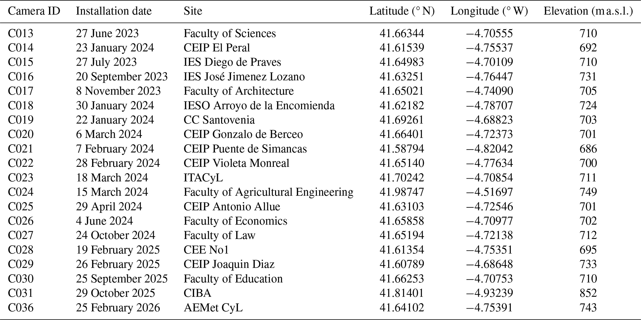
The mentioned network is called PRESENTE as it was developed thanks to a project of the same name. It can be considered as a sub-network within GOA-SCAN (GOA all-Sky CAmeras Network), a bigger all-sky camera network managed by the Group of Atmospheric Optics from the University of Valladolid (GOA-UVa). The PRESENTE network is currently formed by 20 all-sky camera stations (as of February 2026), deployed on public buildings across the city (schools, high schools, university faculties, community centers, among others). The distribution of the stations tries to cover a wide variety of camera distances from more than 50 km to less than 200 m, in order to have different viewing angles of the clouds above them. Two extra cameras are deployed outside the city at 40 and 25 km, in order to assess the capability of the system to retrieve really high clouds (see locations in Fig. 1 and coordinates in Table 1).

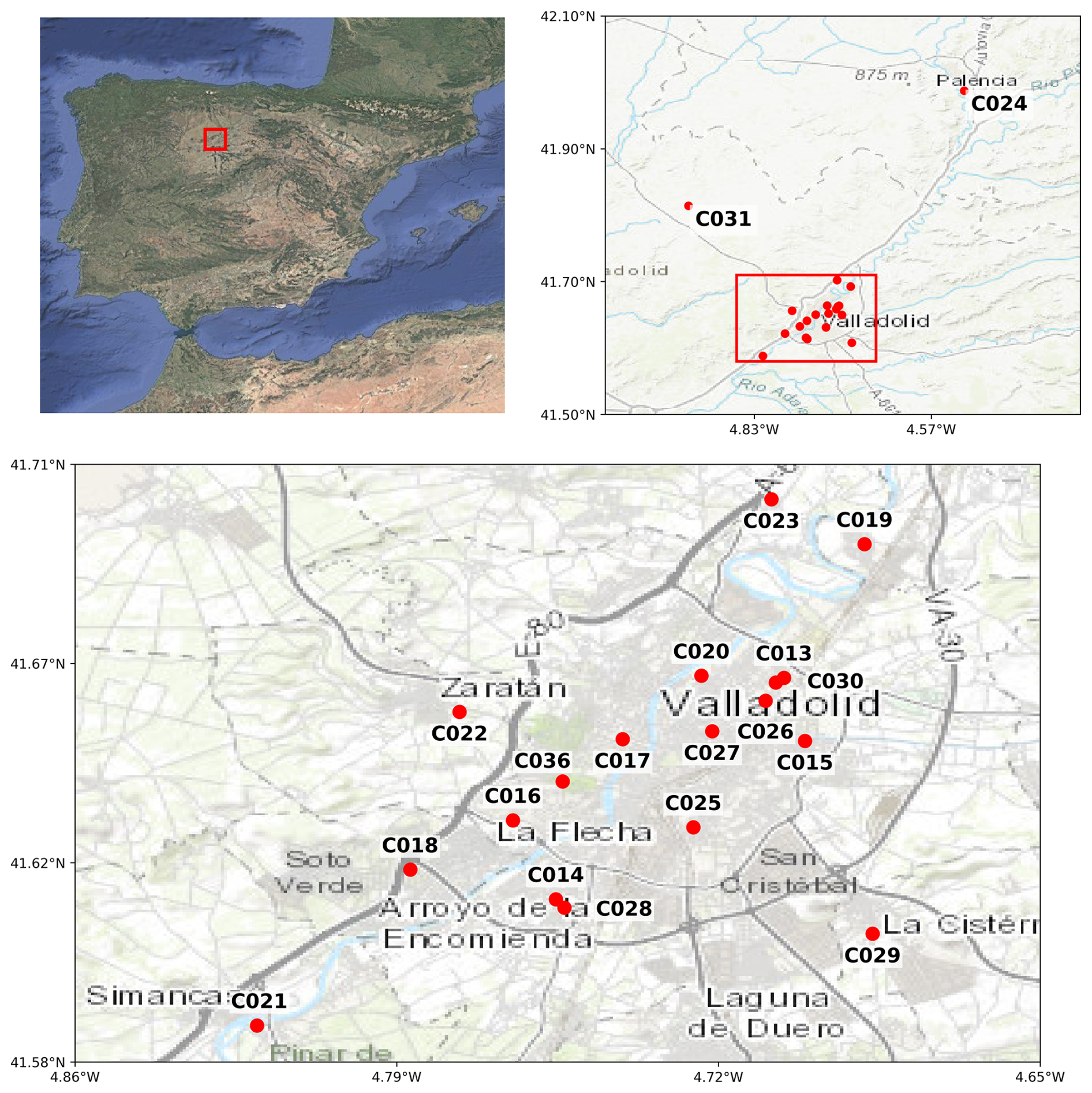
Figure 1 Location of the all-sky cameras of the PRESENTE network. GOA-SCAN identifier for each station can be found in Table 1. Base map: CARTO Positron, data © OpenStreetMap contributors.

Table 1 Details of PRESENTE all-sky camera network. Each instrument is identified by its ID in GOA-SCAN, the installation date and its coordinates. All the installations have been selected in public buildings. CEIP, IES, CEE and CC are the Spanish acronym for public school, public high school, special education school and community center, respectively. All the faculties buildings belong to the University of Valladolid. ITACYL stands for Agricultural Technology Institute of Castilla y León. AEMet CyL refers to territorial delegation of the state meteorological agency and CIBA is the Research Center for the Lower Atmosphere, managed by the University of Valladolid as well.

The all-sky camera model of the PRESENTE network is the OMEA-3C-TF a modified version of the OMEA-3C camera manufactured by Alcor Systems (Román et al., 2025). This camera is formed by a SONY IMX178 CMOS sensor with a fisheye lens, both encapsulated in a weatherproof case with a BK7 glass dome on top, including a heating system to avoid water condensation (González-Fernández et al., 2024). The sensor has three RGB filters (Red, Green and Blue) arranged in a RGGB Bayer pattern mosaic and a triband filter over the sensor (instead of an infrared cutting-off filter like in the OMEA-3C model) in order to reduce the spectral width of each color channel (Román et al., 2025).

These cameras are operated through an external computer placed inside a weatherproof outdoor box. These computers run the GOA OMEA-Capture software (Román et al., 2025), which handles camera configuration, image acquisition, downloading, processing, and data transfer. Following the GOA-SCAN protocols, the PRESENTE instruments are set up to capture a set of multi-exposure raw sky images every five minutes during the daytime and every two minutes at nighttime, which is considered when the solar zenith angle (SZA) is above 97°. For the OMEA-3C-TF model, exposure times are specifically adjusted. At night (SZA>97°), the camera uses, in addition to an ISO amplification set to a gain of 150, a multi-exposure sequence of 1, 5, 10, 20, and 30 s for moonlit nights (when the Moon is between the first and third quarters and the Moon zenith angle below 80°), and 3, 6, 12, 24, and 48 s under moonless conditions. During the day, the sequences depend on SZA: from 0 to 35°, the times are 214, 356, 640, 1208, and 2344 µs; from 35 to 75°, a 4616 µs exposure is added; and finally from 75 to 88°, a 9160 µs exposure is included (Román et al., 2025). These different SZA intervals are set to best adjust to different illumination conditions, also distinguishing fast changes during twilight. To optimize storage without losing coverage of the full sky, the captured images are cropped to 2000×2000 pixels and saved in raw format (14-bit stored in 16-bit format, without demosaicing or white-balance corrections). Each image sequence is stored in a single Hierarchical Data Format version 5 (HDF5) file that also contains the associated metadata. The software is designed to automatically send these files to the GOA-SCAN servers, where they are processed into 8-bits RGB High Dynamic Range (HDR) color images (Antuña-Sánchez et al., 2022; Román et al., 2025). These HDR images are then published on the GOA-UVa website, which provides continuous updates from each station in the network (https://goa.uva.es/proyecto-presente/, last access: 9 September 2026). In this work, all references in the methodology to all-sky images refer to HDR images.

Each GOA-SCAN camera is carefully leveled to face the zenith and geometrically calibrated. This calibration is done with the ORION software (Antuña-Sánchez et al., 2022). This calibration involves identifying the positions of several stars in a set of cloud-free nighttime images, and relating their measured pixel coordinates to their known astronomical coordinates. Using this information, the software reconstructs the camera's pointing geometry by estimating the image center (sky zenith), the azimuthal offset with respect to image north, and the polynomial relationship between radial pixel distance and zenith angle. The resulting calibration matrices allow the precise mapping of any pixel to its corresponding viewing direction (zenith and azimuth coordinates). The GOA-SCAN cameras are subject to regular maintenance, which includes cleaning and inspection and a new geometric calibration is carried out whenever the camera is moved or its orientation shifts, even slightly (Román et al., 2025).

In addition, a semantic segmentation model developed by GOA-UVa and described by Gatón et al. (2026) has been used to provide a segmented sky mask for identifying cloudy pixels in each sky image. This model is named “GOA-UVa All-Sky Segmentation U-Net Model” and it is available in Román et al. (2026). The model segments into five semantic classes: cloud-free, cloud, thin cloud, sun or other. Validation results from Gatón et al. (2026) showed that it achieves a recall of 87 % in the class non-thin clouds and 96 % in the class clear skies. This model was developed for daytime images, but is also used for nighttime images in this work.

2.2 Ceilometer

Ceilometers are single-wavelength lidar-based instruments designed to continuously monitor the vertical structure of the lower atmosphere and widely used to determine the CBH. They operate by emitting short laser pulses upward and measuring the backscattered signal returned by aerosols, cloud droplets, and other atmospheric constituents (Herrero del Barrio et al., 2024). The CBH is generally estimated as the height for the local maxima in the backscatter signal or in its vertical gradient, allowing the detection of one or multiple cloud layers depending on atmospheric conditions (Martucci et al., 2010). The ceilometer model used in this study is a Lufft CHM15k-Nimbus, which operates with a pulsed 1064 nm Nd:YAG laser and provides continuous vertical backscatter profiles at 15 m resolution up to 15 km above ground level (a.g.l.). Two different instruments are used, one installed on the same rooftop as the C013 camera, and the other one at CIBA location as the C031 camera (see Table 1). Both are part of the ICENet network, and their data are calibrated and processed following ICENet operational protocols (Cazorla et al., 2017). These instruments are configured to provide a range-corrected signal every 15 s. They can provide CBH and cloud penetration depth (CPD) products at three different height levels with the same temporal resolution. From these parameters, the CTH can be estimated by adding the CPD to the CBH at each corresponding level. However, according to the manufacturer's specifications (Lufft, 2021), the CPD represents the depth into the cloud at which the laser signal is fully attenuated. Therefore, CTH values calculated this way are only fully reliable if the ceilometer detects an additional cloud layer above the current one, which guarantees that the laser has completely penetrated the first layer. In many cases, especially with low and dense clouds, the signal may be extinguished before reaching the actual top or any higher layers. In such instances, the CPD does not represent the total cloud thickness, and the resulting CTH must be handled with caution as it likely underestimates the real cloud top.

2.3 Satellite imagery

The Sentinel-2 mission, part of the European Space Agency (ESA) Copernicus Programme, provides high-resolution optical imagery for monitoring land and coastal environments. It is composed of two identical satellites, Sentinel-2A and Sentinel-2B, which fly in the same sun-synchronous orbit separated by 180°. Together, they achieve a swath width of 290 km and a revisit frequency of approximately five days under identical viewing geometry; in higher latitudes or overlapping orbits, this frequency can increase (Obregón et al., 2019).

Each satellite carries a MultiSpectral Instrument (MSI) that records reflected solar radiation in 13 spectral bands spanning from the visible and near-infrared (VNIR) to the shortwave infrared (SWIR) regions. The data are provided at three spatial resolutions: 10 m for four bands, 20 m for six bands, and 60 m for three bands. The 60 m bands are primarily designed for atmospheric correction and cloud detection operations (Drusch et al., 2012). The Sentinel-2 true color product is generated by directly mapping the reflectances of bands B4 (red), B3 (green), and B2 (blue) into an RGB image (Sovdat et al., 2019).

The Scene Classification Layer (SCL) product, provides a per-pixel mask with 60 m resolution that efficiently detects clouds, snow, and cloud shadows, producing a classification map that includes four cloud-related classes (including cirrus) and six surface classes (shadows, vegetation, bare soil/desert, water, and snow). It operates on Level-1C Top-of-Atmosphere (TOA) reflectances at 60 m resolution and generates additional quality indicators expressing the probability of cloud or snow occurrence. To optimize performance for operational processing, the algorithm relies on a sequential filtering approach that combines spectral thresholds, band ratios, and normalized indices such as NDVI and NDSI to identify potential cloudy pixels. These pixels undergo successive spectral tests in which the cloud probability is iteratively updated, ranging from 0 (high-confidence cloudless sky) to 1 (high-confidence cloud). The sequence terminates when the probability drops to zero, classifying the pixel as cloud-free. This probabilistic framework allows the algorithm to be computationally efficient and robust under varying illumination and atmospheric conditions. A self-organizing neural network (SOM) is also used in later steps to refine cloud and shadow classification. This classification is introduced into Sen2Cor processing chain, which performs the atmospheric correction used to generate level-2A products (Richter et al., 2012). In this work, the Sentinel-2 true color and SCL products corresponding to tile 30TUM, defined within the Military Grid Reference System (MGRS) and covering the Valladolid region, have been downloaded from the Copernicus Data Space Ecosystem.

3 Methodology

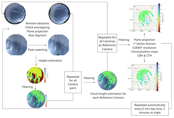
This section describes the proposed methodology for computing the cloud heights maps (specifically CBH and CTH) from the simultaneous all-sky images, from the mentioned PRESENTE network, captured at a given time. The procedure for image processing, cloud height computation, and cloud height map generation is explained. This algorithm can be implemented continuously to process the pictures taken by all the all-sky cameras of the network. It is important to remark that by using various camera pairs with different baselines, the system captures parts of the vertical cloud structure, enabling the retrieval of both CBH and CTH. For each grid bin, the minimum and maximum retrieved cloud heights are assigned to CBH and CTH, respectively. It should be noted, however, that cameras observe clouds from the surface; consequently, CTH calculation is expected to be less accurate and precise than CBH, as the top part of the clouds is often obstructed by the cloud layer itself and is only visible from a few viewing angles.

3.1 Two images approach

3.1.1 Image rectification

To enable the inter comparison of fisheye images, the following procedure is implemented. First, a camera from the network is chosen as the reference camera and its image is paired with the corresponding image captured by another camera. For clarity, this second camera is denoted as the auxiliary camera in this description.

The Sun and surrounding objects, such as buildings, trees, and street lamps, are removed from both sky images by filtering out the saturated pixels and applying a custom made mask indicating the position of these obstacles for each camera. Also, a zenith angle control threshold is defined as θ_t=75°. In both sky images, pixels with zenith angles exceeding this threshold are discarded, since such viewing geometries are expected to introduce larger errors in the subsequent stereoscopic cloud height retrieval.

Then the geographical coordinates of the cameras are used to compute the relative displacement between both cameras. With this distance between the cameras on a local cartesian system (Δx, Δy), it is possible to obtain the relative orientation angle between the reference and auxiliary camera as: $\mathit{\beta }=\arctan \left(\frac{\mathrm{\Delta }x}{\mathrm{\Delta }y}\right)$. After that, both the reference and auxiliary fisheye images are transformed into planar projections. This is possible due to the geometrical calibration parameters of each camera. As mentioned in Sect. 2.1, the geometrical calibration provides the azimuth and zenith angles from which each pixel is viewed by the camera, but also the pixel coordinates of the zenith (camera center) and the relationship between the pixel radial distance (r) to this center position and the sky zenith angle (θ); this relationship is given by the coefficients of a second order polynomial. In a first step, the azimuth angles are corrected by an azimuth offset (Δϕ) to align with north-up. To obtain the planar projections of the images, a Cartesian grid with uniform spacing and same resolution as the input image is generated at a fixed height. In this work, the grid is defined as a 4 km square at Z=0.6 km above the camera. This grid is oriented according to the angle β relative to the North, ensuring that both images are projected into the same reference system. This alignment is crucial as it enables a direct pixel by pixel comparison along the rows of both planar images. For each point in the grid (X,Y), the corresponding zenith and azimuth angles are calculated knowing the height and distance from each point to the center of the grid $\left(\mathit{\theta }=\arctan \left(\frac{\sqrt{X^{\mathrm{2}}+Y^{\mathrm{2}}}}{Z}\right),\mathit{\varphi }=\arctan \left(\frac{X}{Y}\right)\right)$. Then the polynomial r(θ) and the azimuth offset Δϕ are used to get the pixel coordinates from the viewing angles ($u=u_{\mathrm{0}}-r\left(\mathit{\theta }\right)\sin (\mathit{\varphi }+\mathrm{\Delta }\mathit{\varphi })$, $v=v_{\mathrm{0}}-r\left(\mathit{\theta }\right)\cos (\mathit{\varphi }+\mathrm{\Delta }\mathit{\varphi })$, where x₀, y₀ are the optical center coordinates obtained from the calibration). Finally, bilinear interpolation is performed on these pixel values (u, v) for each channel of the RGB image, evaluating each pixel of the original fisheye image.

The projected image is then resampled to produce the oriented planar view. To optimize computational efficiency, the planar image is downsampled to a resolution of $\mathrm{200}\mathrm{pixels}\times \mathrm{200}\mathrm{pixels}\times \mathrm{3}\mathrm{pixels}$. This significantly reduces processing time while preserving an adequate compromise between spatial resolution and the quality of the resulting cloud height retrieval. Figure 2 shows an example of two fisheye images taken at the same time for two cameras of the network, with the masked obstacle objects and the saturated pixels colored black (A1, B1), their planar projection (A2, B2) and the oriented planar projection so that the rows of both images align (A3, B3). Note that, since the images are acquired from the ground looking upward, the East–West axis appears reversed with respect to conventional maps, so that the North direction remains oriented upward. From this point, the algorithm only works with these rectified images.

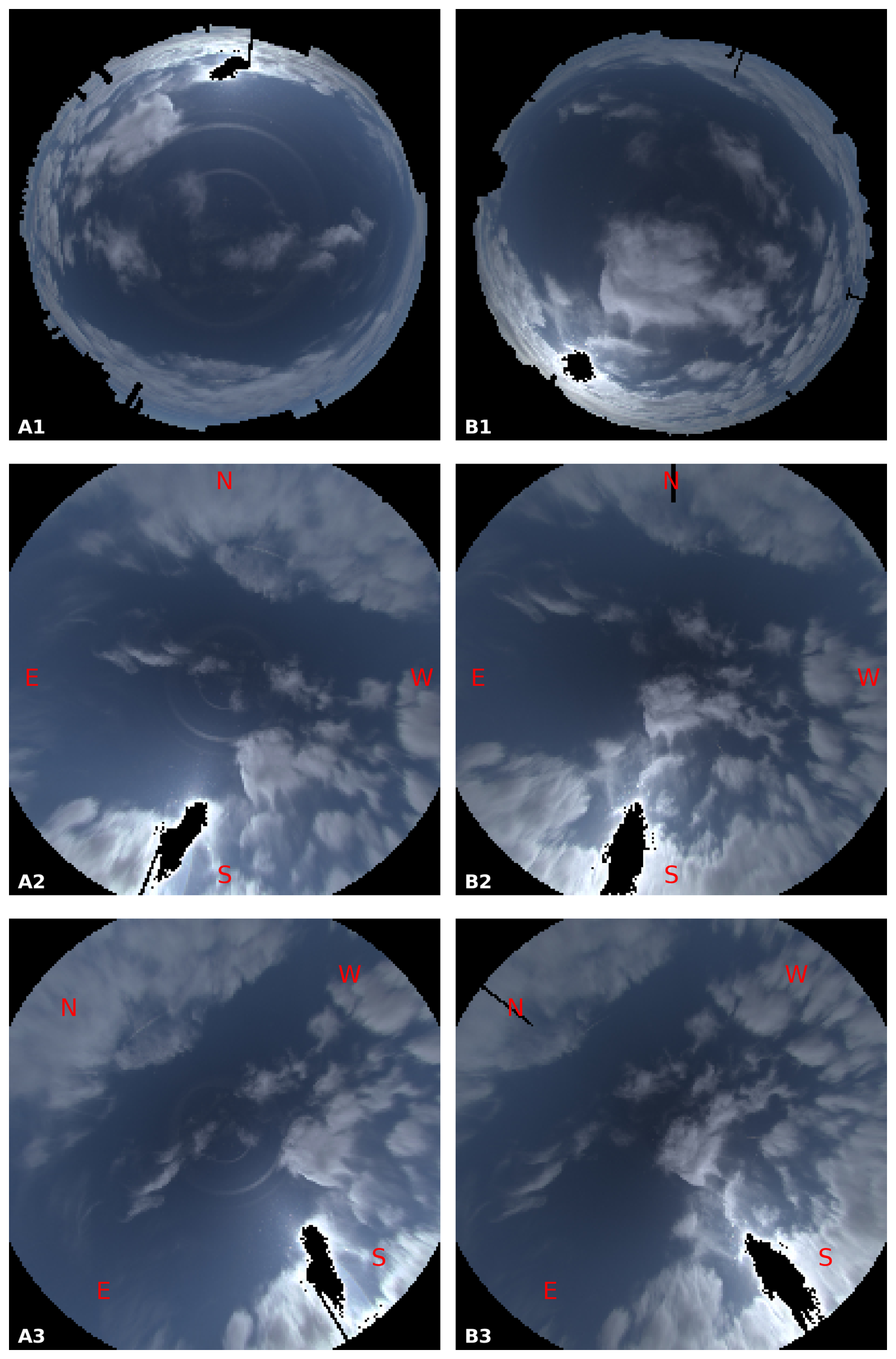
Figure 2 Sky images captured by cameras C013 and C014 on 28 December 2025 at 11:20 UTC. It is shown: fisheye original HDR all-sky images, with the obstacle objects and the sun saturated pixels colored black (A1, B1), their planar projection oriented upside to North (A2, B2) and their planar projection oriented so the rows of both images align (A3, B3).

3.1.2 Pixel matching and cloud height estimation

Once the pair of images (reference and auxiliary) is rectified, the next step is to identify the pixels of the reference image in the auxiliary one. As it can be seen in Fig. 2, the rows of the oriented plane image A3 are coincident with the rows of B3, so corresponding points are constrained to lie along the same image row (row-wise correlation). To improve the pixel correlation with the information of the surrounding pixels, a square window centered on each selected pixel in the reference image is extracted. The window size used is 7 pixels×7 pixels. For each valid window (all 49 pixels in the window are not masked or saturated in any color channel) in the reference image (Fig. 2A3), the algorithm searches for the most similar valid window along the same row in the other camera image (Fig. 2B3). The similarity between the reference window and each candidate window in the auxiliary image is quantified using the sum of the normalized cross-correlation of each color channel, providing a value, hereinafter referred to as RGB-correlation, between −3 and 3. For each pixel sampled in the reference image, the position of the pixel with the maximum RGB-correlation coefficient in the auxiliary camera image is stored. This provides: a maximum RGB-correlation coefficient matrix, storing the mentioned correlation values, and a pixel-column position matrix, recording the pixel column location in the auxiliary image where the best match (maximum RGB-correlation) is found (see Fig. 3). As shown in Fig. 3A, lower correlation values are generally observed in clear sky regions, while the highest values typically occur at cloud edges. These features provide distinct textures that are more easily identified by the matching algorithm than the more homogeneous appearance of both the clear sky and the cloud interior. Regarding the pixel-column position matrix (Fig. 3B), the spatial variation of the values is smoother in areas with high RGB-correlation, indicating a consistent and continuous displacement field across the cloud structures. Conversely, in regions of low correlation, the pixel-column position values are noisier, which typically indicates inaccurate pixel matching.

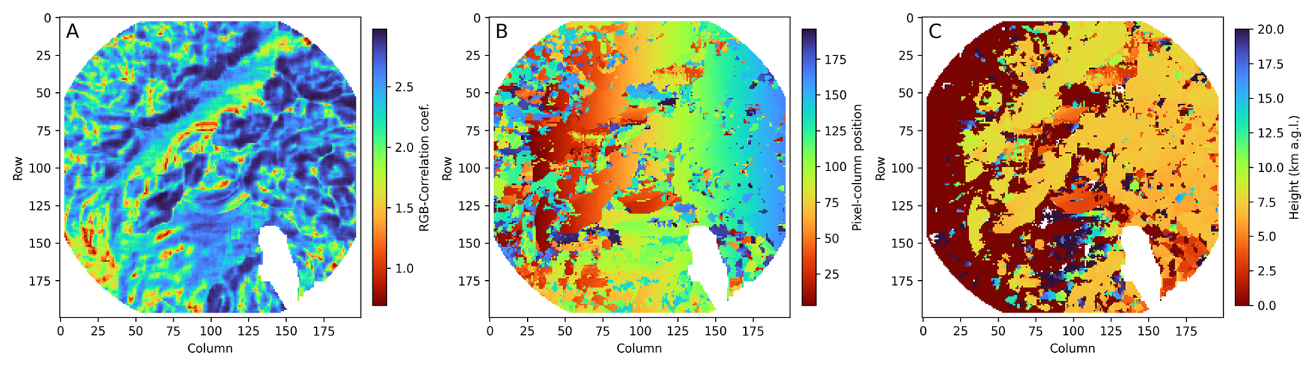
Figure 3 For the same camera pair and timestamp as Fig. 2, maximum RGB-correlation coefficient MATRIX (A), pixel-column position matrix (B) and height matrix (C). To improve visibility, the color bar limits are truncated for the maximum RGB-correlation coefficient matrix (A) and for the cloud height matrix (C).

The zenith (θ) and azimuth (ϕ) viewed by each reference pixel (i,j) and its correspondent pixel in the auxiliary image (i,k) (where k is obtained in the mentioned column position matrix), are well known. Figure 4 shows a schematic representation of a camera pair pointing to the same spot (C), where the index A corresponds to the reference camera and the index B to the auxiliary camera. From this disposition, Eq. (1) can be derived (same index notation used), which gives the altitude (H) above sea level ($\mathrm{a}.\mathrm{s}.\mathrm{l}.$) of the observed point. The altitudes of each camera are denoted as h_A and h_B, Δx is defined as the longitudinal distance between the camera pair and ϕ_A, ϕ_B, and θ_A, θ_B are the respective azimuth and zenith angles.

$$\begin{array}{}\text{(1)}& {\displaystyle }{\displaystyle }H={\displaystyle \frac{h_{\mathrm{B}}\cdot \sin \left({\mathit{\varphi }}_{\mathrm{B}}\right)\cdot \tan \left({\mathit{\theta }}_{\mathrm{B}}\right)-h_{\mathrm{A}}\cdot \sin \left({\mathit{\varphi }}_{\mathrm{A}}\right)\cdot \tan \left({\mathit{\theta }}_{\mathrm{A}}\right)-\mathrm{\Delta }x}{\sin \left({\mathit{\varphi }}_{\mathrm{B}}\right)\cdot \tan \left({\mathit{\theta }}_{\mathrm{B}}\right)-\sin \left({\mathit{\varphi }}_{\mathrm{A}}\right)\cdot \tan \left({\mathit{\theta }}_{\mathrm{A}}\right)}}\end{array}$$

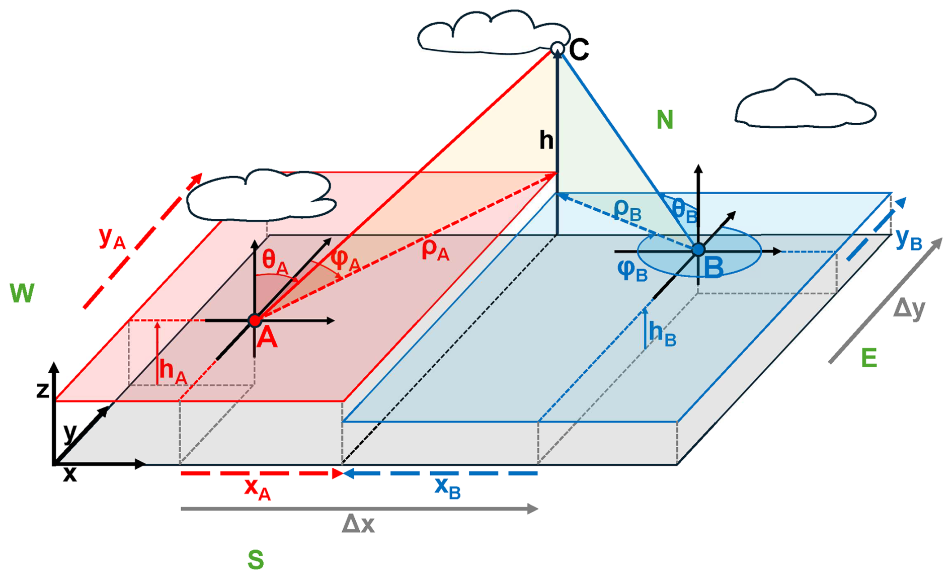
Figure 4 Schematic representation of the system geometry for a camera pair pointing to the same cloud point (C). The index A is used for variables corresponding to the reference camera, while the index B indicates the auxiliary camera. Here, θ represents the zenith angle, ϕ is the azimuth angle, H denotes the height of cloud point C above sea level ($\mathrm{a}.\mathrm{s}.\mathrm{l}.$), and Δx indicates the longitudinal distance between both cameras in km.

Alternatively, H could be calculated from the latitudinal difference (Δy) using the following Eq. (2):

$$\begin{array}{}\text{(2)}& {\displaystyle }{\displaystyle }H={\displaystyle \frac{h_{\mathrm{B}}\cdot \cos \left({\mathit{\varphi }}_{\mathrm{B}}\right)\cdot \tan \left({\mathit{\theta }}_{\mathrm{B}}\right)-h_{\mathrm{A}}\cdot \cos \left({\mathit{\varphi }}_{\mathrm{A}}\right)\cdot \tan \left({\mathit{\theta }}_{\mathrm{A}}\right)-\mathrm{\Delta }y}{\cos \left({\mathit{\varphi }}_{\mathrm{B}}\right)\cdot \tan \left({\mathit{\theta }}_{\mathrm{B}}\right)-\cos \left({\mathit{\varphi }}_{\mathrm{A}}\right)\cdot \tan \left({\mathit{\theta }}_{\mathrm{A}}\right)}}\end{array}$$

Although Eq. (1) was used throughout this study, Eq. (2) is recommended whenever the absolute value of Δx is smaller than that of Δy. An improved approach to be considered in future work, which explicitly accounts for uncertainties in the identified viewing angles (ϕ_A, θ_A, ϕ_B, and θ_B), would be to estimate the H values by minimizing the distance between the two lines of sight corresponding to each camera, as defined by the viewing angles ϕ_A and θ_A, and ϕ_B and θ_B, respectively.

Figure 3C shows an example of the obtained cloud heights for each matching pixel in the auxiliary image. It is important to keep in mind that a cloud height value is calculated even for cloud-free pixels, although these will be removed in subsequent processing steps. As observed in this panel, retrieved heights in cloud covered areas show realistic values around 7 $\mathrm{km}\mathrm{a}.\mathrm{g}.\mathrm{l}.$, whereas cloud-free pixels typically yield unrealistic values, such as negative heights or values exceeding 20 km. This preliminary height map already provides a first approximation for distinguishing between cloudy and cloud-free pixels on the basis of the physical consistency of the stereoscopic retrieval.

The uncertainty in the retrieved cloud height values is obtained by slightly shifting ±1 pixels the column positions of the maximum RGB-correlation coefficient value in the auxiliary image. For each displaced position, the cloud height is recalculated using Eq. (1). Finally, for each pixel, the absolute differences between the original cloud height and the ±1 recalculated values are computed and the maximum of these two is considered as the uncertainty on the retrieved pixel cloud height. This uncertainty is greater than the uncertainties derived from zenith and azimuth because the error from these angles is around 1–2 pixels (Antuña-Sánchez et al., 2022), whereas in this case, because of the image downsizing, the ±1 pixel shift corresponds to ±10 pixels in the original image.

3.1.3 Two-images cloud height filtering

To ensure the reliability of the retrieved cloud heights, several filtering criteria are applied. First, physically plausible cloud heights thresholds are imposed: pixels with cloud height values below the ground level of the reference camera or above 15 km (a.g.l.) are removed. This upper limit is chosen because most clouds are expected to lie within the troposphere, and higher values are likely cloud-free pixels or artifacts of the calculation rather than real cloud heights.

In addition, a range of admissible altitudes is defined based on the distance between the two cameras. This range is directly proportional to the distance between the cameras (d), since the overlapping field of view of two pairs of cameras is more sensitive to lower clouds when the cameras are closer together, and to higher clouds when they are farther apart. The minimum and maximum values of the admitted range are defined as the heights that would be seen from one camera to the other with angles between 80° and 10°, respectively $\left(H_{\text{min}}=\frac{d}{\tan \left(\mathrm{80}\right)},H_{\text{max}}=\frac{d}{\tan \left(\mathrm{10}\right)}\right)$.

Also, cloud height values whose associated uncertainty exceed the chosen threshold of 1 km are also discarded. The error in the assumed height will be 1 km with this threshold; this is a conservative choice, however, in many cases the actual error should be smaller. The quality of the pixel matching is then considered: cloud heights derived from pixels with a RGB-correlation coefficient lower than an established threshold of 2.25, or from undefined values, are rejected, as these cases correspond to poor or ambiguous correlations. Finally, the calculated segmentation sky mask (see Sect. 2.1) of the reference image is used to restrict the analysis to pixels identified as cloudy (cloud and thin cloud classes), thereby avoiding spurious correlations in cloud-free regions.

This process yields an estimation of cloud heights by stereoscopic calculations using a pair of cameras, with one of them designated as the reference camera. Due to the imposed filtering criteria, these cloud heights can be considered to represent reliable cloud points. To allow direct comparison of the cloud points matrices obtained from different pairs, all results must be expressed in the same reference system. For this purpose, the rotation applied earlier to align the image rows is reversed. The matrices are rotated around the image center, aligning the products with the external reference frame (north-up) and the camera viewing geometry. To these matrices, the same filters described earlier, based on geometrical consistency, physical plausibility, and correlation thresholds, are applied in order to remove unreliable values. The result is a set of 200×200 geometrically consistent cloud height, correlation, and uncertainty matrices that can be directly compared between different camera pairs with the same reference camera.

3.2 Multi-image processing

The procedure described in Sect. 3.1 is repeated pairing the reference camera with each of the others available in the network. Since the fields of view of multiple cameras may overlap depending on cloud heights, a filtering process is proposed to avoid redundant data and ensure computational efficiency. For each pair of all-sky cameras, the overlap area of their two vision cones (defined by θ_t=75°) is evaluated at a range of discrete height levels (0.5–15 $\mathrm{km}\mathrm{a}.\mathrm{s}.\mathrm{l}.$, in 0.5 km increments). A camera pair is only considered valid if the overlapping area at a given height level represents between 20 % and 80 %. Specifically, at each height level, it is checked whether the overlapping area has already been covered by a previously processed pair. If the new pair does not increase the overlapping area by at least 5 % at any height level, it is excluded from the calculation.

Figure 5 illustrates the cloud points and their heights retrieved for the reference camera C015 at 11:20 UTC on 28 December 2025, when paired with all the different available cameras that fulfill the overlapping criteria. From Fig. 5, it can be observed in practically all camera pairs, that the clouds identified in the image are located at an altitude of approximately 7 $\mathrm{km}\mathrm{a}.\mathrm{s}.\mathrm{l}.$, with some pixels showing slightly lower heights toward the North. However, certain discrepancies arise depending on the specific auxiliary camera used. These differences may be attributed to several factors, such as geometric calibration uncertainties or optical reflections within the camera domes. Despite these minor variations, the cameras providing the most reliable results are those separated from C015 by distances between approximately 5 and 10 km. In contrast, very few valid cloud height estimates are obtained from camera C031, which lies more than 30 km away from the reference C015 camera. There are also less valid cloud points for camera C026, which is located too close to the reference C015 camera, less than 2 km away. In both cases, the stereoscopic cloud height retrieval deteriorates: for C031, the cameras observe the cloud field from excessively different points, so their fields of view have little overlap, while for C026 the images are too similar for the given cloud height (around 7 $\mathrm{km}\mathrm{a}.\mathrm{g}.\mathrm{l}.$), displacement values are really small, limiting the accuracy of the cloud height retrieval.

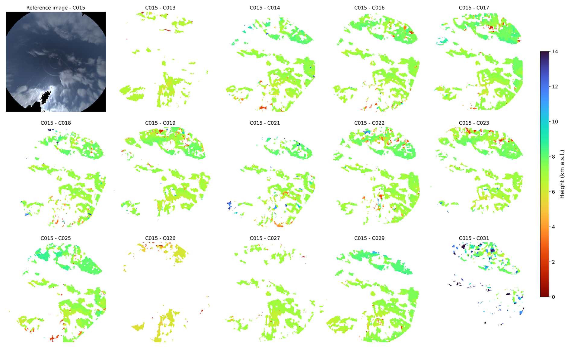
Figure 5 Estimation of cloud height for reference camera C015, after pairing with each one of the available cameras which fulfil the overlapping criteria at 11:20 UTC on 28 December 2025. The first panel (top-left) shows the north-up oriented planar projection of the reference C015. The subsequent panels display the retrieved cloud height maps derived from correlating the reference image with each auxiliary camera, as specified in the titles.

In order to minimize the uncertainties in the derived cloud height values, the median value of the cloud height estimates from the different camera pairings is obtained for each pixel of the reference camera. The formed image with these median values is considered as the cloud height matrix for the reference camera. For the case analyzed in Fig. 5, this would be the median value of all the cloud height matrices shown from the pairing of each all-sky camera available with C015. This approach provides a robust estimate while reducing the influence of noisy or outlier results from individual camera pairs.

To these cloud height estimations obtained for a given reference camera (the mentioned median of all individual pairs results), an additional filtering procedure is applied to refine the results and remove spurious values. First, a median filter with a 3×3 window is applied, and the difference between the filtered and original matrices is calculated. Pixels that deviate by more than 1 km from the local median are discarded, in order to remove isolated outliers and warranty smoothness between adjacent pixels. Next, a layer filtering step is applied. A frequency histogram is computed from the remaining cloud height values, with 1 km bins between 0–15 km (a.g.l.). Then up to four height layers are selected from this distribution corresponding to the most populated bins, retaining only those containing at least 2 % of the valid pixels. The centers of these bins are interpreted as the dominant cloud layers. All pixels whose height differs by more than 0.7 km from the center of every selected layer are discarded, ensuring that only cloud heights consistent with the main layers in the scene are preserved.

The effect of these two filters is to discard outliers, suppress isolated noisy pixels, and smooth the retrieved cloud height distributions while preserving, if existing, the different cloud height layer structure. The result for the case in Fig. 6C shows that the filtered heights are spatially coherent and smooth, replicating the shape shown in the camera image and discarding spurious values produced by abnormal highlighted artifacts.

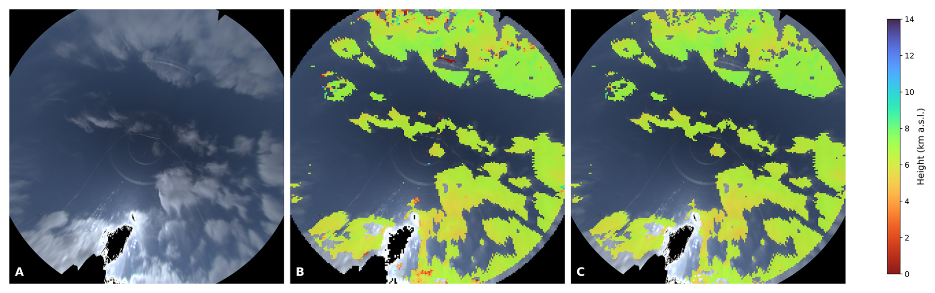
Figure 6 Panel (A) shows the planar projected image from the C015 camera on 28 December 2025 at 11:20 UTC. Panel (B) includes over this image the cloud height median values from all the available camera pairs with C015 camera (see Fig. 5). Panel (C) represents the same panel (B) but after applying the 3×3 median and layer filters.

As explained previously, the image size is reduced to a 200×200 grid in order to optimize the computational time required for the correlation calculations between images. These reduced matrices are resized to the original 2000×2000 resolution using nearest-neighbor interpolation in order to include information for all cloudy pixels of the original image.

Once the cloud points and their heights have been determined for a given reference camera, the procedure is repeated using a different camera as the reference. In this sense, each camera in the system is successively designated as the reference camera, and the same stereoscopic reconstruction and filtering steps are applied. The process continues until every camera has been the reference, yielding a set of cloud fields estimations equal in number to the set of reference cameras.

Figure 7 illustrates the results obtained for each of the cameras in the analyzed case. Cameras C020 and C028 were not working due to malfunctions, C024 is excluded from the plot because it shows few representative cloud heights due to the large distance regarding the rest of the cameras, and C036 was not installed yet. Almost all of them successfully identify a fractured mid height cloud stratum. The retrieved cloud heights are homogeneous through the images, particularly in the central region of the sky image of each camera. There is a decrease in the resolution for the fragmented clouds near the horizon. This is a consequence of the projection geometry and the reduction in effective pixel resolution at high zenith angles, which limits the precision of the correlation process at the edges of the images. In the case of camera C031, the distance to the other cameras prevents it from seeing this range of clouds heights, since the overlapping field of view between cameras is not enough. Only a few pixels from the sky image are correlated with pixels in other cameras' images and maybe there are some wrong correlated pixels that yield on higher altitudes. In the Supplement, Fig. S1 shows another case of interest where it can be seen how the different camera distances in the network can facilitate the retrieval of different cloud layers within the same scene. This Fig. S1 reveals a high level cloud layer with lower level cumulus clouds beneath it. While both structures are not visible in all camera views, they are clearly distinguished in those where they both appear; this points out that the camera network's high density and spatial distribution provide multiple perspectives of the cloud field, enabling distinct cloud layers to be effectively differentiated.

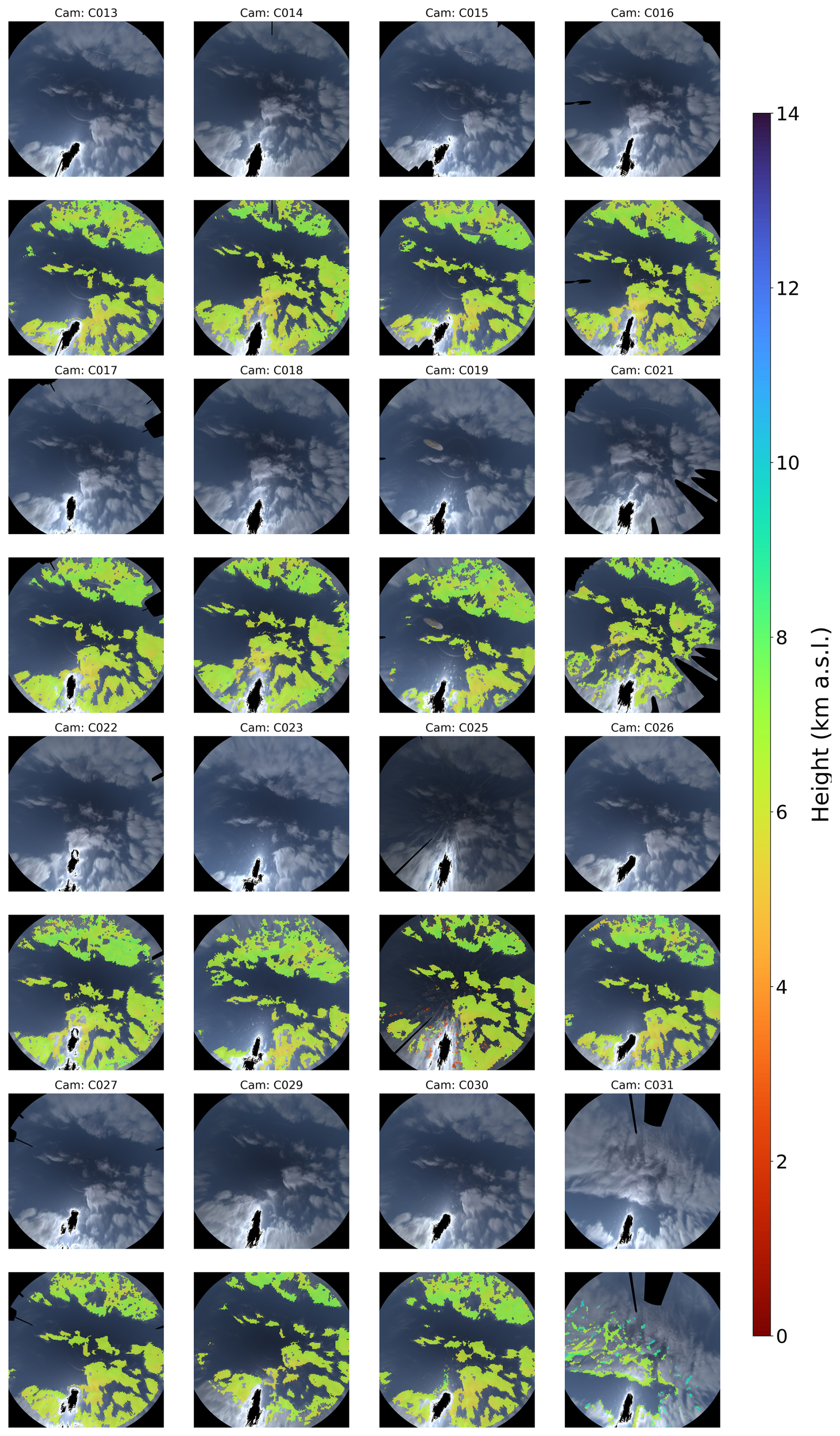
Figure 7 Cloud height values obtained for all cameras available at 11:20 UTC on 28 December 2025. For each camera, a pair of vertically aligned subplots is presented: the upper image displays the north-up oriented planar projection of the original sky scene, while the lower image shows the same projection with the estimated cloud height values overlaid. The color scale represents the retrieved altitude ($\mathrm{km}\mathrm{a}.\mathrm{g}.\mathrm{l}.$).

3.3 Cloud height grid

For each reference camera, the final cloud point pixels are converted to georeferenced coordinates using the zenith, azimuth and cloud height information of each pixel. The chosen reference system is a local cartesian centered in the coordinates of the C013 camera (see Table 1). To spatially aggregate the retrieved cloud points, a regular geographic grid is defined centered in the C013 camera coordinates. This grid covers a domain of ±0.5° in both longitude and latitude and is discretized in bins with a resolution of 0.0005°. This results in a two-dimensional array of bins, for which both the geographical limits and the central coordinates are explicitly determined. At these spatial scales, the geometric distortions associated with Earth curvature are negligible, this may become relevant when cameras are separated by several kilometers or when clouds reach high altitudes. Nevertheless, the results obtained from implementing this correction have proved to be quite equivalent, so the more simple calculation is implemented in the automation of cloud height retrieval to increase speed and reduce computational cost.

Each available cloud point from all reference cameras, its cloud height estimation and the ID of its corresponding reference camera, is then assigned to one of these grid bins. Points falling outside the defined grid are discarded. Thus, for each bin of the grid, there is a number of cloud points, from one or more reference cameras, which will exhibit a specific cloud height distribution for that bin. For each bin, a set of statistics is computed, including the number of different reference cameras providing cloud points to the bin, the maximum, minimum and the standard deviation of the cloud height distribution of the bin and the number of cloud points obtained within this bin. These statistical estimators allow a robust characterization of the variability within each grid bin while also providing a measure of the confidence offered by multiple camera perspectives.

Figure 8A shows the number of cameras that contribute with at least one cloud point to each grid bin. The highest overlap appears in the central region of the network, where multiple cameras have overlapping fields of view. In contrast, peripheral areas are only seen by a few cameras. Figure 8B displays the total number of individual cloud points assigned to each bin. Higher counts indicate regions where the stereoscopic retrieval is most reliable due to strong camera overlap. Lower counts highlight areas with limited observations or pixels removed by the quality filters. It is important to note that the number of data points per bin typically decreases as cloud altitude increases. This is because, for a given viewing angle, the physical area covered by each pixel expands with height, causing the available data to be distributed over a larger surface area. Based on these distributions and in order to ensure the reliability of the aggregated information, only grid bins meeting two criteria are retained: at least two distinct cameras must contribute to the bin, and there must be four or more individual cloud points inside it. These threshold values were manually selected based on an empirical review of the results. While they provide a robust filter for this study, they are not necessarily the most optimal in all scenarios, as the ideal thresholds likely depend on the density of the camera network and the altitude of the clouds being observed. This filtering guarantees that the resulting grid highlights only those regions supported by sufficient sampling, effectively reducing the impact of outliers. The outcome is a set of gridded cloud height maps that are spatially consistent and directly suitable for subsequent analysis and visualization.

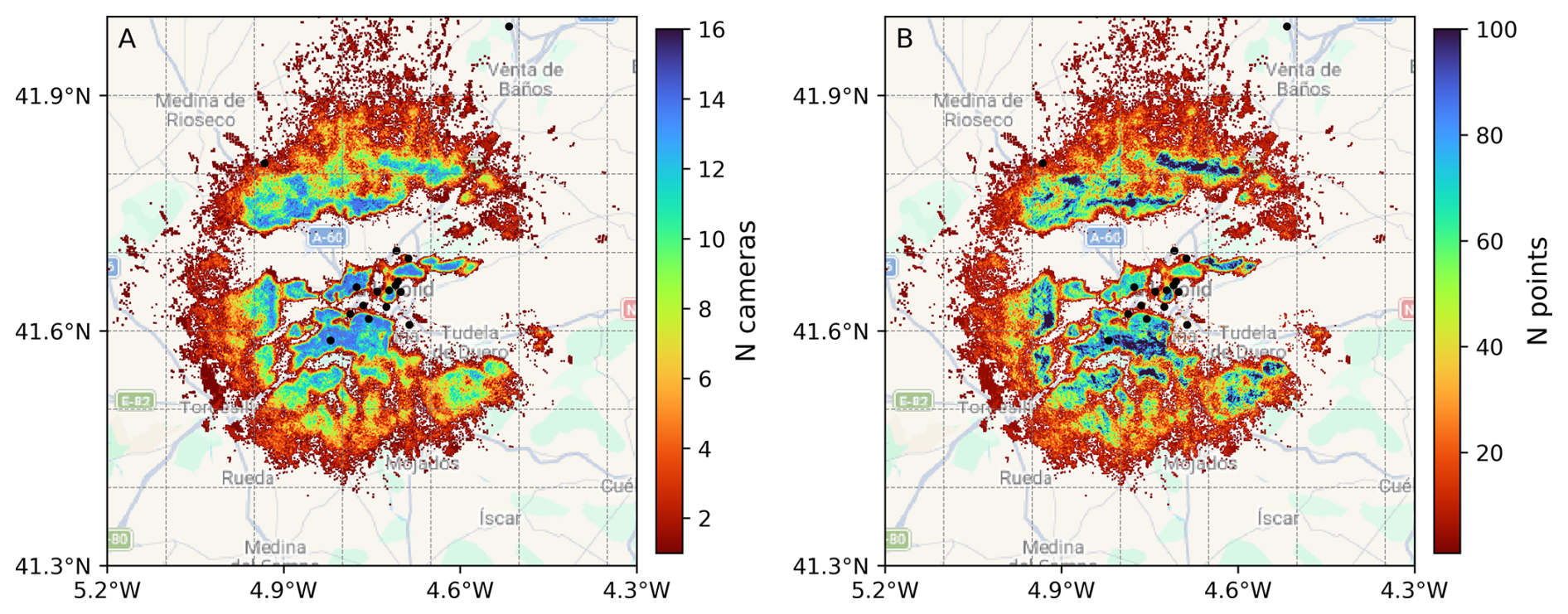
Figure 8 Number of cameras providing cloud points (A) and number of cloud points (B) for each bin of the latitude–longitude grid. White dots indicate the locations of the cameras that contribute to the stereoscopic calculation (28 December, 11:20 UTC).

Figure 9A shows the minimum height values retrieved, hereafter referred to as the CBH, for the analyzed case. In this example, the CBH remains relatively constant around 7 $\mathrm{km}\mathrm{a}.\mathrm{s}.\mathrm{l}.$, although slightly lower values are observed in the central region of the map. Figure 9B presents the maximum cloud heights within each grid bin, hereafter denoted as the CTH. These values are generally centered around 8 $\mathrm{km}\mathrm{a}.\mathrm{s}.\mathrm{l}.$, even though some isolated bins show abnormally high values that likely correspond to spurious data. Figure 9C illustrates the standard deviation of all height estimates within each grid bin. Higher standard deviation values indicate increased variability in the retrieved cloud point heights within a given bin. This variability is typically associated with multilayer cloud structures, although in some cases it may also reflect the presence of residual outliers (e.g. the aforementioned spurious CTH values). Notably, the standard deviation is lower in the central part of the grid. This may be attributed to a more precise characterization resulting from the higher number of cameras covering this area; however, it could also be related to the viewing geometry, since these clouds are located in the central part of the images, it is more challenging to distinguish their vertical edges and thickness compared to more slanted views. Together, these three cloud products provide a consistent description of both the vertical structure and the spatial variability of the reconstructed cloud field. Based on these three parameters, it can be concluded that the analyzed cloud layer appears highly homogeneous around 7 km and relatively thin, with differences between top and base heights approximately of 1 km, and with the standard deviation of the heights remaining low, roughly 0.2 km, except for some localized areas in the northern sector. Similarly, in the Supplement, Fig. S2 presents a more complex scenario where the methodology effectively distinguishes distinct cloud levels within the same field of view. In this case, the retrieved heights reveal cloud structures at altitudes between 10–12 $\mathrm{km}\mathrm{a}.\mathrm{s}.\mathrm{l}.$, while other regions of the map show clouds at much lower levels, around 2 $\mathrm{km}\mathrm{a}.\mathrm{s}.\mathrm{l}.$ This example confirms the system's ability to identify and separate distinct cloud layers.

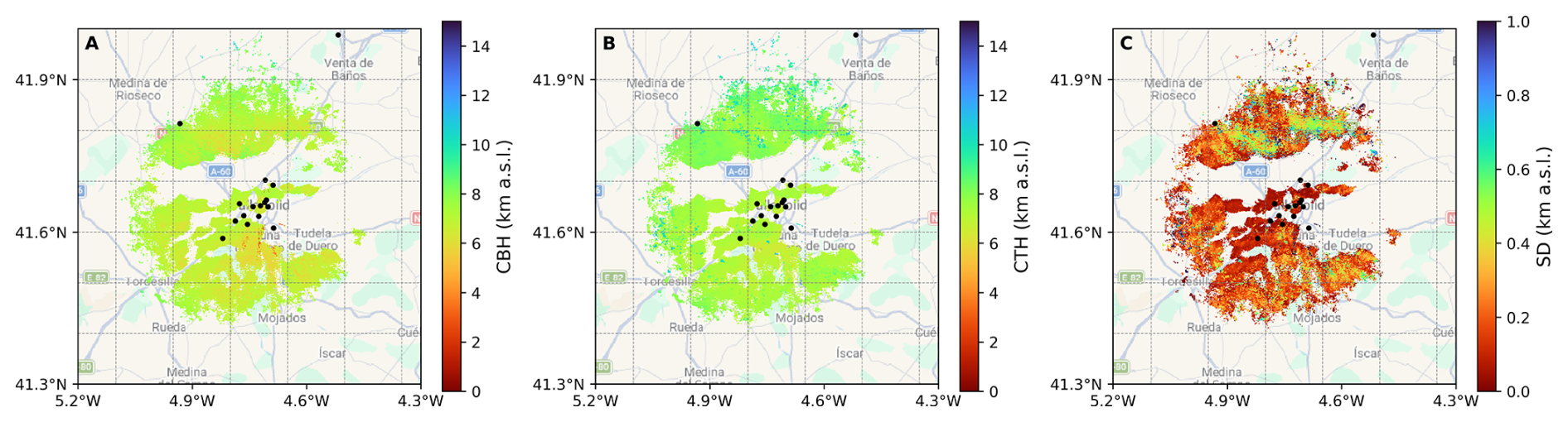
Figure 9 Panel (A) values for cloud base height (CBH), panel (B) cloud top height (CTH) and panel (C) standard deviation of the cloud point heights within each bin of the latitude–longitude grid. White dots indicate the locations of the cameras that contribute to the stereoscopic calculation (28 December 2025, 11:20 UTC).

To fully assess the accuracy of these results, they must be compared against independent measurements from other instruments. For this purpose, the following section presents a validation study using the CBH and CTH products derived from the methodology applied to the entire historical image record available, comparing them with data from independent ground based and satellite sensors.

4 Validation of cloud estimations from the all sky camera network

4.1 Comparison with Sentinel-2 cloud mask

Satellite imagery and ground-based all-sky cameras provide complementary perspectives of the cloud field. The proposed stereoscopic method provides cloud height estimates with high temporal resolution at the local/regional scale, while some polar satellite instruments, such as Sentinel-2, offer an overhead view with robust cloud detection but lower temporal resolution. By comparing both datasets, it has been possible to assess whether the cloud structures estimated from the camera network are consistent with the distribution of clouds observed from space.

For a qualitative comparison of the cloud maps obtained from the all-sky camera network with those derived from Sentinel-2, both datasets have been evaluated on a point to point basis. Sentinel-2 SCL (60 m) has been first filtered to obtain the different cloud classes (medium probability, high probability, and thin cirrus). The cloud mask retrieved from the all-sky has been obtained for a geographical grid as explained in Sect. 3. To ensure spatial consistency, this Sentinel-2 cloud mask has then been resampled to the camera network's geographical grid using the nearest neighbor interpolation method. This has allowed each grid point to be directly compared and classified as cloudy or cloud-free if there was an available cloud height value or not, respectively.

Figure 10 shows the mentioned Sentinel-2 SCL product at 60 m resolution and its comparison with the all-sky cameras cloud mask, for the particular case, which has been analyzed in the previous section (28 December 2025 at 11:20 UTC). A large fraction of the cameras' retrieved cloud field agrees with medium and high-probability cloud classes in the SCL layer (green pixels), confirming that the camera network captures the main cloud structures, which can also be distinguished in the satellite true-color image. The differences between both datasets have been found mainly at cloud borders. One possible explanation for this is the difference in contrast between cloud and cloud-free pixels and land and cloud pixels, which could make the Sentinel-2 algorithm discard more cloud values in the edges of the clouds where transparency is high. On the other hand, satellites have an almost zenithal point of view of the clouds, whereas cameras observe clouds from different angles. This implies that the level of detail captured depends on the cloud's position in the image; a cloud located near the zenith (the center of the image) is captured with much finer detail than when it is observed near the horizon. This leads to lower sensitivity for the reconstruction algorithm, especially for small, fragmented clouds. In addition, the width of fragmented clouds frequently prevents observing the cloud-free space between them, which can cause an overestimation of the cloud cover, especially between cloud edges. The cloud height is a key factor determining this sensitivity; higher structures are visible over a wider spatial extent and are therefore sampled by a larger number of cameras, leading to a more homogeneous and robust reconstruction of the cloud field, although the quality of the retrieved product also depends on the distance between the cameras. In contrast, mid and low clouds are observed over a more limited common field of view, so fewer cameras contribute to the same grid bins, making the reconstruction more sensitive to outliers. It can be seen in Fig. 8A, that pixels located at cloud borders coincide with grid bins where the number of contributing cameras is lower, even if the minimum threshold of more than two cameras contributing per bin is satisfied. Although these pixels pass the imposed filtering criterion, the reduced spatial overlap suggests increased uncertainty in the retrieved classification and height at these transition regions. Additionally, the satellite acquisition time does not exactly match the time of the camera images. Even short temporal offsets can result in small displacements of cloud structures, primarily affecting the cloud edges. Nevertheless, the blue regions indicate a robust agreement in cloud-free detection, confirming that the stereoscopic algorithm does not produce significant false positives in cloud-free zones and the discrepancies are found mostly at the transitions between the clouds. Furthermore, the Sentinel-2 SCL product, generated via the Sen2Cor algorithm, presents well-documented limitations. Recent evaluations demonstrate that Sen2Cor's cloud and shadow detection frequently misses thin clouds, partial clouds, and transparent cloud boundaries (Liang et al., 2024). Comprehensive accuracy assessments, including validations using the global CloudSEN12 dataset, show that Sen2Cor significantly underperforms in overall accuracy and F1-scores when compared to both alternative physical-rule-based algorithms (like Fmask or MAJA) and modern spatial-temporal machine learning models such as Cloud Score+ (Aybar et al., 2022; Cal, 2026). Consequently, the discrepancies observed at the cloud edges may partly stem from the satellite mask's own misclassifications rather than solely from stereoscopic reconstruction uncertainties.

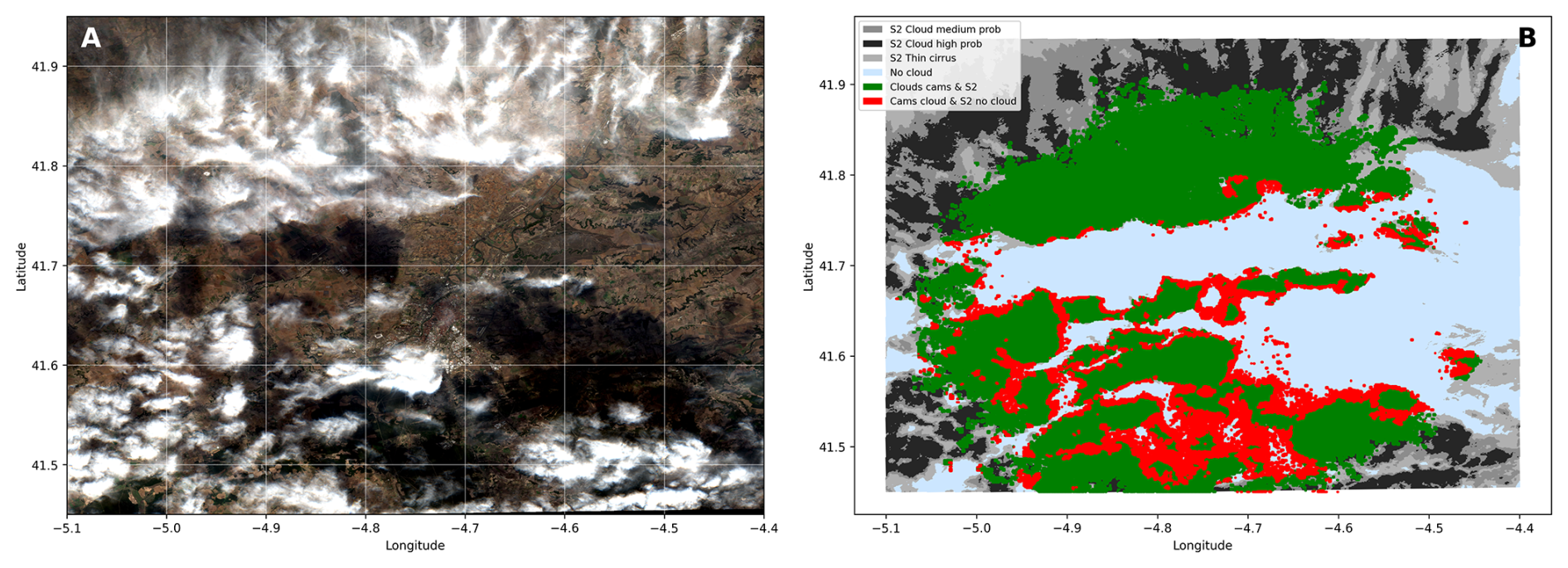
Figure 10 At 28 December 2025, 11:20 UTC: Sentinel-2 true color product (A) and cloud mask obtained from the camera network, together with the Sentinel-2 scene classification product (B). Red points represent cloud height values from the all-sky camera network that Sentinel-2 does not classify as clouds. Green points represent areas where both the all-sky cameras and Sentinel-2 agree that there are clouds. The different shades of grey represent the different cloud scenes classified by Sentinel-2 that the cameras do not detect. Blue represents cloud-free regions predicted by both datasets.

The field of view of the network can also be observed for the present cloud heights, as clouds above 41.9° N latitude are not visible. In the central part of the network, the higher camera density results in shorter camera distances, which ensures strong overlap and reliable detection of low to mid level clouds. Moreover, these central cameras can be combined with more distant peripheral stations, providing larger camera distances that improve the triangulation geometry for higher cloud layers within the same region of the map. In contrast, grid bins located near the outer boundary of the network do not benefit from this geometric complementarity. While clouds in these bins may be observed by nearby stations within the central part of the network, they lack additional outer stations that could provide overlapping views from the opposite side. Consequently, the stereoscopic configuration becomes geometrically constrained toward the perimeter, particularly affecting the reconstruction of lower cloud layers.

Overall, this simple qualitative comparison points out the robustness of the proposed method to detect cloud points with high spatial resolution, identifying the same cloud systems detected by Sentinel-2 at least in the case shown. Discrepancies are largely confined to cloud edges, where fewer cameras see the same cloud point, blind zones, and slight temporal offsets between datasets increase uncertainty.

4.2 Ceilometer cloud heights comparison

For a more quantitative analysis of the retrieved CBH and CTH values with the cameras, the results have been compared with the independent measurements from the mentioned ceilometer installed in the Science Faculty of Valladolid, collocated with the C013 camera, in the center of the defined cloud grid. The cloud height maps derived from the all-sky camera network have been first projected onto a common geographic grid with a spatial resolution of 0.0005° in both latitude and longitude as explained in the previous section. Specifically, the CBH and CTH values that have been used in this comparison correspond to the grid bin closest to the ceilometer's location, which represents the central bin of the grid. To account for the different integration times when matching both datasets, all ceilometer observations within a ±30 s window have been considered, selecting the CBH or CTH value closest to the camera's estimate. Also, nocturnal camera timestamps have been shifted 45 s to better align them with the center of the exposure interval, that increases for low light conditions, ensuring a more accurate temporal match with the ceilometer data. The analysis covers the period from 27 July 2023 to 19 January 2026. During this time, 377 647 paired ceilometer and camera measurements have been taken, excluding those matches for which the ceilometer presented a sky condition index (SCI) indicating precipitation, fog, snow, reduced window transmission or malfunction.

Table 2 summarizes the performance of the camera network against the ceilometer for cloud detection. Of all cases where the cameras have identified clouds in the ceilometer's grid bin, they agree with the ceilometer in 95 % of times, indicating a very low false positive rate. In contrast, cameras have correctly identified 59 % of the clouds reported by the ceilometer. The remaining 41 % of clouds detected by the ceilometer but missed by the cameras are primarily due to the ceilometer's ability to operate in nearly all conditions. On the one hand, there are limitations related to very low clouds and overcast conditions, also cases not classified as fog by the ceilometer. While the ceilometer identifies the presence of a cloud layer at very low altitudes, the cameras often fail due to a lack of image texture and contrast, as the images are quite homogeneous and is difficult to find high RGB-correlations. Furthermore, at such low altitudes, there may be no overlap between the field of view of any cameras from the network. On the other hand, there are limitations related to the detection algorithm under specific lighting conditions, it should be noted that the segmentation algorithm used to discard outliers was not originally designed for nocturnal conditions, where it tends to misclassify clouds as cloud-free sky; this even happens sometimes for very dark clouds during daytime. Regarding the few cases (3 %) where the cameras have detected clouds but the ceilometer has reported cloud-free skies, these are likely due to external factors such as dust deposition on the camera, or dome reflections that may be misclassified as clouds. It is also important to note that since the methodology requires a minimum of two reference cameras viewing cloud points in the same bin and applies height constraints based on camera distances, some cloud cases detected by the ceilometer are filtered out for the cameras network by these quality criteria. This is particularly relevant during the periods when only two cameras were operational (almost two months at early stages of the network, see installation dates in Table 1); causing many of these missed detections. Despite these limitations, the agreement in cloud-free scenarios has remained remarkably high at 97 %.

Table 2 Comparison of cloud and cloud-free detections between the camera system and the ceilometer using the punctual data at the ceilometer coordinates as the reference. The values represent the number of data points where both systems coincide or differ, with the percentages relative to the total number of detections in each ceilometer category shown in parentheses.

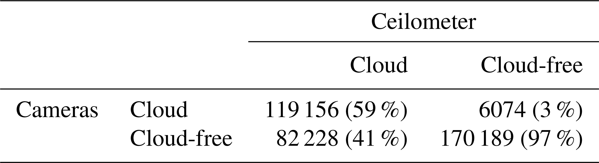
Figure 11 shows the outcome of extending this comparison to the cloud height values estimated by both instruments. The plots show a notable difference between CBH (panels A, B) and CTH (panels C, D) analysis. Results for CBH show a high correlation with a determination coefficient (R²) about 0.89. The majority of the data points are concentrated at low altitudes (<2 $\mathrm{km}\mathrm{a}.\mathrm{g}.\mathrm{l}.$) and align closely with the 1:1 line, confirming the strong agreement between both independent datasets. Some dispersed points are observed where the camera network underestimates the CBH compared to the ceilometer. The mean bias error (MBE) calculated as the mean of the differences (ΔCBH) between camera and ceilometer values, is remarkably low (−0.19 km), indicating high accuracy, as the camera network predicts the CBH at an altitude very similar to the ceilometer on average. This can also be seen in the histogram of CBH differences (Fig. 11B), which shows a Gaussian-like distribution centered at zero. Approximately 25 % of the differences fall within ±0.2 km, and about 35 % are within ±0.4 km. The Standard Deviation (SD) of the differences is 1 km, which establishes the precision of the method at approximately this value for the current network configuration. Furthermore, the Root Mean Square Error (RMSE) is 1.02 km, nearly identical to the SD because the MBE is close to zero. This value reflects the impact of the dispersed points observed in Fig. 11A, although most of the data remains closely aligned with the 1:1 line, as is indicated by the pixel density values.

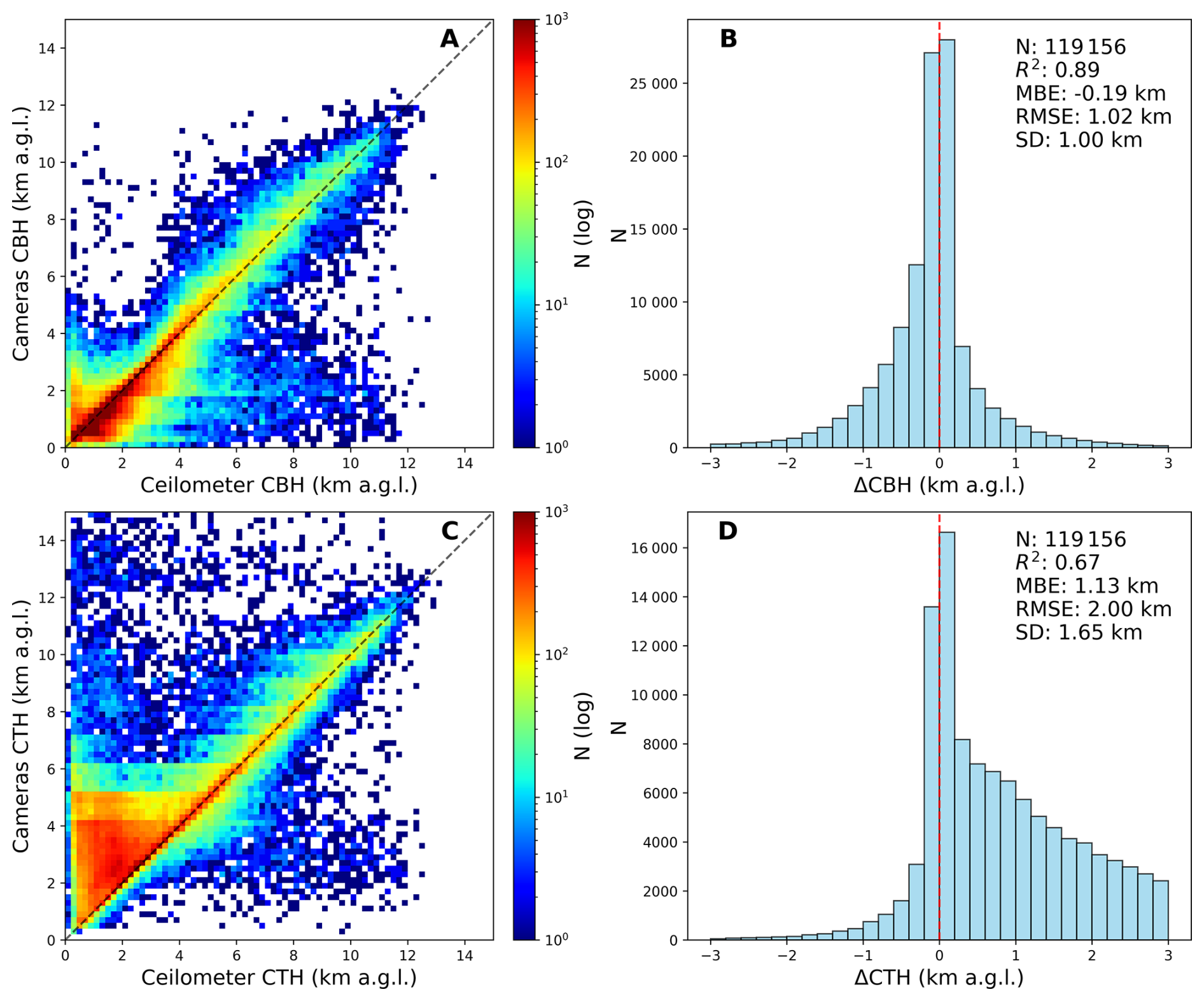
Figure 11 Bidimensional frequency histogram of camera values against ceilometer ones for cloud base height (CBH) and cloud top height (CTH) in panels (A) and (C), respectively. Colorbar represents the number of data of each bin in a log scale. Panels (B) and (D) represent the frequency histogram of the differences (ΔCBH and ΔCTH) between both instruments. Statistical metrics provided include the total number of cases (N), coefficient of determination (R²), mean bias error (MBE), root mean square error (RMSE) and standard deviation (SD).

Regarding the CTH, Fig. 11C shows that the camera network and ceilometer also correlate, though with a lower R² value of 0.67. While many observations still fall close to the 1:1 line, there is significantly more dispersion compared to the CBH analysis. The cameras tend to yield higher CTH values than the ceilometer for low ceilometer CTH values. This discrepancy is likely due to two factors: first, the ceilometer signal often saturates in low, thick clouds, potentially underestimating the cloud width, and consequently the CTH, but also failing to detect higher layers and thus underestimating the true CTH. Second, the limitation of the cameras as the top part of the cloud is only visible from fewer viewing angles. This trend is reflected in the histogram of differences (Fig. 11D) by a prominent right-shifted tail of positive values. Despite this, the highest frequency of differences remains centered near 0 km. The mentioned overestimation in low cloud scenarios results in a higher MBE of 1.13 km. The precision of the CTH measurements degrades compared to the CBH as SD increases to 1.65 km. Consequently with these MBE and SD values, the RMSE rises to 2 km, reflecting the increased dispersion in the CTH compared to the CBH.

To ensure a more consistent comparison between the camera network and the ceilometer, a spatial averaging approach has been implemented. Initially, the cameras' cloud heights have been extracted from the single grid bin at the ceilometer's location. However, this isolated bin may not fully represent the ceilometer's measurement, which is integrated over a 15 s interval, whereas the camera acquisition is quasi-instantaneous during daytime and longer than the ceilometer at nighttime. As clouds move during these temporal offsets, a single spatial point can result in discrepancies. To account for this and achieve a more robust comparison, the grid bins within a 150 m radius of the ceilometer location (31 bins in total) have been considered to be a more representative area. The median and standard deviation of these bins have been calculated for each obtained CBH and CTH maps, separately. This median values provide a more realistic information of the cloud height retrievals from the cameras, but in order to ensure the reliability of this dataset, the following filtering criteria has been applied: for each defined grid bin, if there are less than 20 height values within the selected area (31 bins), those values and their median are discarded.

Using this new spatial representativeness criterion, the matching process with the ceilometer data has been repeated following the same procedure as the point to point analysis. In this approach, an observation is classified as cloud-free if no valid cloud height is retrieved among all the bins within the mentioned 150 m radius window. These results, presented in the first row of Table 3, show an overall agreement of 66 % predicting clouds, which represents an improvement over the point to point comparison. The case when cameras detected clouds not identified by the ceilometer remains the same at only 3 %.

Table 3 Comparison of cloud detection by the camera network, validated against the ceilometer as the reference instrument, under various solar zenith angle (SZA) ranges. Camera detections are based on the median cloud height value within a 150 m radius of the Valladolid ceilometer location. Rows represent different lighting conditions: SZA 0–180° (all conditions), SZA 0–80° (daylight), SZA 80–110° (twilight), SZA 110–180° (night), and SZA 110–180° night with moon presence. Filtering criteria have been applied to discard heights provided by two or fewer cameras and with fewer than 20 height values. The values represent the number of data points where both systems coincide or differ, with the percentages relative to the total number of detections in each ceilometer category shown in parentheses.

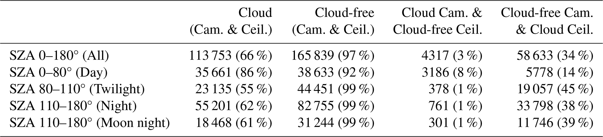
Since the illumination conditions seem to affect noticeably the cameras measurements and the performance of the segmentation model, an analysis of the cloud detection depending on the SZA is presented in Table 3. For daylight conditions the system achieves its peak performance, with the highest cloud detection coincidence of 86 %. In this regime, the high contrast and clear image texture of the images allow for easy visualization and identification of clouds, with high RGB-correlations. The performance of the cloud segmentation algorithm in retaining cloudy pixels is also significant. On the other hand, a higher number of cases where the cameras predict clouds not identified by the ceilometer (8 %) has been found during daytime. This is likely due to the strong presence of the sun in these images, which produces significant saturation if not obstructed by clouds (one example of this can be seen in Fig. S1 Cam C017 in the Supplement). Furthermore, direct solar radiation makes reflections and dirt on the camera dome more apparent (see in the Supplement Figs. S3 and S4 for an example of a dirty dome case); these features can generate high but fictitious RGB-correlations, leading to artifacts and the retrieval of non real clouds in the final product. The performance of cloud detection for the cameras degrades during twilight, close to sunset and sunrise (SZA between 80 and 110°); while the agreement for cloud-free scenarios remains exceptionally high at 99 %, the cloud detection coincidence drops to its worst performance (55 %), with missed clouds increasing to 45 %. Under these conditions, where most of the solar radiation becomes diffuse, the cloud-free sky and the clouds are difficult to distinguish even visually. Consequently, the segmentation model is unable to correctly identify many clouds, increasing the underestimation of cloud presence by the camera method compared to the ceilometer. This highlights the challenges of quick light intensity transitions where the signal to noise ratio decreases, as the exposure times need to be increased. For the nighttime data, there is a 62 % agreement for cloud presence, while 38 % of clouds identified by the ceilometer are missed by the camera network. Interestingly, when filtering for night with moon presence (SZA 110–180° Moon night), the detection accuracy remains similar at 61 %, suggesting that moonlight does not fully compensate for the limitations of the segmentation algorithm and the lower contrast compared to daytime images. Moreover, nocturnal sky images exhibit greater variability between cameras than daytime images due to the influence of nearby artificial light sources; these spatial differences in illumination can also cause the proposed cloud identification algorithm to perform worse under these conditions. Notably, the rate of cases where cameras detect clouds not identified by the ceilometer is lower for twilight and nighttime conditions (1 %). This discrepancy supports the hypothesis that these infrequent false detections are primarily driven by dome reflections and dirt and dust deposition; such factors are significantly more impactful under direct solar illumination, whereas their influence is minimized during the night.

To study the performance of the proposed methodology to retrieve the CBH and CTH values, Figs. 12 and 13 show the mentioned cloud height median values by the camera compared to the measured by the ceilometer for the different illumination regimes. Figure 12 shows the results for CBH, presented in columns A (bidimensional frequency histogram) and B (histogram of differences). Figure 13 shows the results for CTH, following the same structure for the whole dataset in columns A and B, and additionally including, in columns C and D, the subset of cases where the CPD is considered reliable – that is, when an additional cloud layer is detected above, as specified by the manufacturer (see Sect. 2.2). This comparison complements the results of Table 3, showing not only whether clouds are detected, but also how precise the measurement of their altitude is. To ensure the reliability of the spatial averaging approach, an additional filtering criterion has been applied: any CTH or CBH median value with a standard deviation above 1 km within the <150 m area of the grid has been discarded. This ensures the homogeneity of the median value, as cases with multiple cloud layers at different altitudes within the same 150 m radius area could yield unrealistic median estimates for ceilometer comparisons.

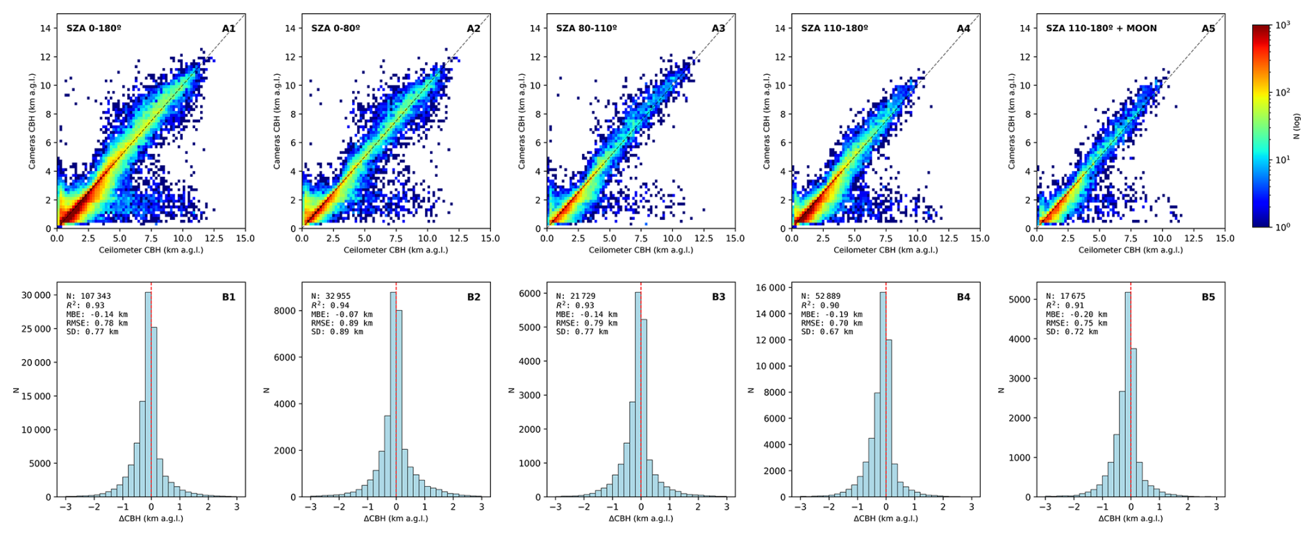
Figure 12 First row (A) presents the bidimensional frequency histogram of median cloud heights values from the camera network within a 150 m radius of the Valladolid ceilometer location, against ceilometer values for cloud base height (CBH). Second row (B) presents the frequency histogram of the differences (ΔCBH) between both instruments. Filtering criteria have been applied to discard heights provided by two or fewer cameras, with fewer than 20 height values and a standard deviation higher than 1 km. Rows represent different lighting conditions: SZA 0–180° (all conditions), SZA 0–80° (daylight), SZA 80–110° (twilight), SZA 110–180° (night), and SZA 110–180° (night with moon presence). Results include total number of cases (N), coefficient of determination (R²), mean bias error (MBE), root mean square error (RMSE) and standard deviation (SD).

The results show a significant improvement in correlation compared to the single pixel analysis; for the all conditions dataset, the determination coefficient increases to 0.93 for CBH and to 0.72 for CTH. Regarding the different illumination regimes, for CBH, the highest determination coefficient is found during daylight conditions (R²=0.94; Fig. 12A2), as expected. However, the CTH shows the highest correlation values during twilight (R²=0.77; Fig. 13A3) and moonlit nights (R²=0.77; Fig. 13A5), surpassing the daytime correlation (R²=0.68; Fig. 13A2). Although the camera network's detection sensitivity decreases at night and twilight (highest rates of missed detection respect to the ceilometer), it consistently measures the height of the clouds it successfully identifies. Consistent with the previous central pixel analysis, the data pairs for both CBH and CTH remain primarily concentrated around the 1:1 line, as evidenced by the high density of points in the panels A1–A5 in Fig. 12 and A1–A5 in Fig. 13. However, the CTH exhibits higher dispersion, particularly at lower cloud heights, likely for the same reasons discussed in the point to point analysis of Fig. 11: the ceilometer signal saturates in low, thick clouds, preventing it from detecting higher cloud layers. When restricting the comparison to cases where the CPD is considered reliable (Panels C and D in Fig. 13), the overestimation of the CTH by the cameras is notably less pronounced. For the all conditions dataset, R² increases from 0.72 to 0.80 and the MBE decreases from 1.06 to 0.52 km (Panel D1), while the RMSE decreases from 1.78 to 1.21 km. This improvement is consistent across illumination regimes. This suggests that the observed overestimation at lower levels, while statistically significant, might not be entirely an artifact of the camera system, but could also be due to the ceilometer's lack of sensitivity to higher cloud layers when obscured by optically thick low-level clouds. However, restricting the validation to the filtered subset alone would be overly strict, as it would discard a substantial number of cases in which the ceilometer signal reached a single cloud with no additional layer above it, that the ceilometer fully penetrates. For this reason, both the unfiltered and CPD filtered results are presented.

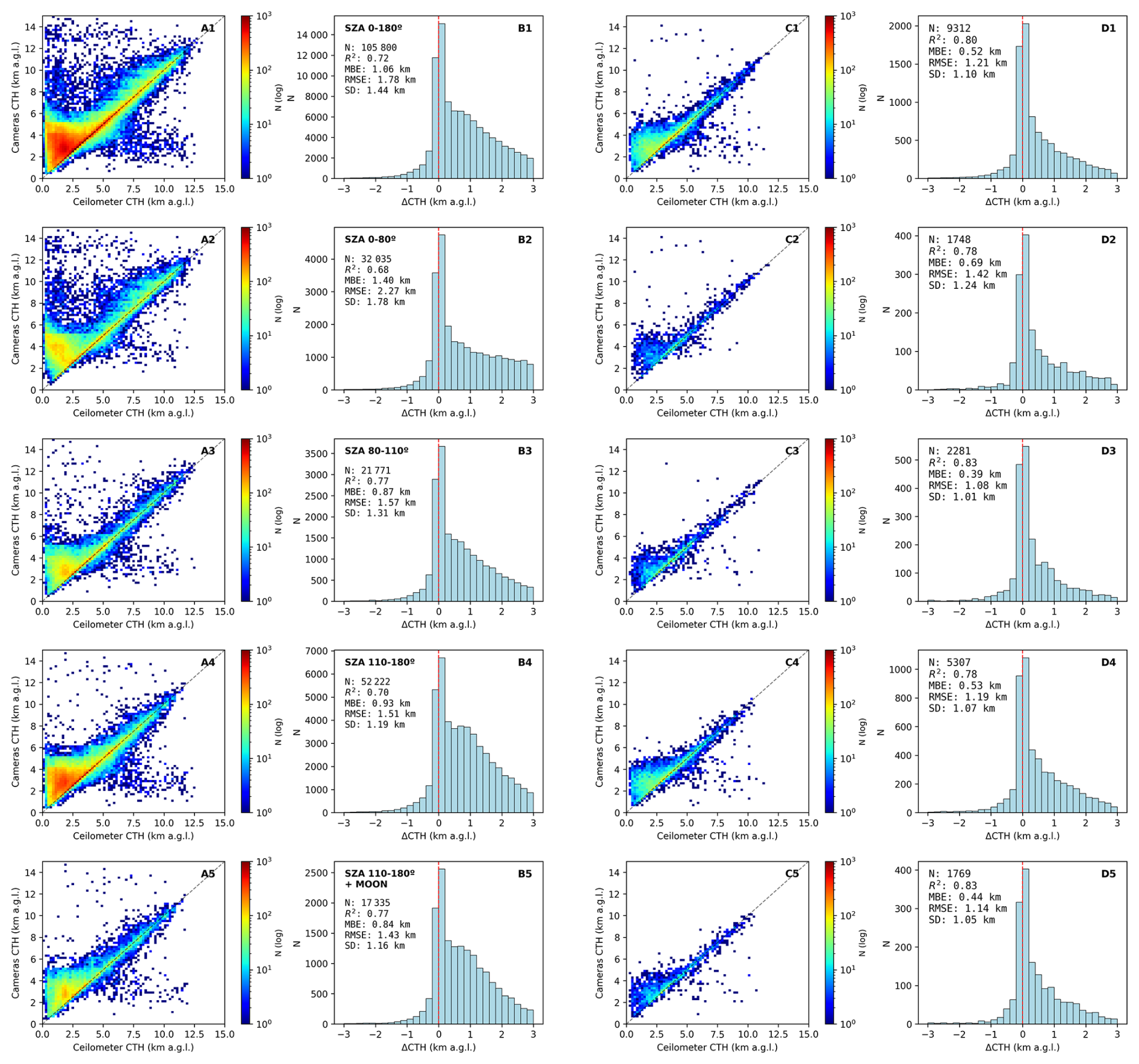
Figure 13 Bidimensional frequency histogram of median cloud heights values from the camera network within a 150 m radius of the Valladolid ceilometer location, against ceilometer values for cloud top height (CTH) in panels (A) and (C), respectively. Panels (B) and (D) represent the frequency histogram of the differences (ΔCTH) between both instruments. For columns (C) and (D), only those cases where the signal successfully penetrated the cloud layer, according to the manufacturer's criteria mentioned in Sect. 2.2 have been included. Additional filtering criteria have been applied to discard heights provided by two or fewer cameras, with fewer than 20 height values and a standard deviation higher than 1 km. Rows represent different lighting conditions: SZA 0–180° (all conditions), SZA 0–80° (daylight), SZA 80–110° (twilight), SZA 110–180° (night), and SZA 110–180° (night with moon presence). Results include total number of cases (N), coefficient of determination (R²), mean bias error (MBE), root mean square error (RMSE) and standard deviation (SD).

Regarding the accuracy for the entire dataset, the CBH shows a MBE value of −0.14 km, whereas the unfiltered CTH shows a MBE value of 1.06 km. For CBH distinguishing different illumination intervals, the highest accuracy occurs during daytime, with an MBE of −0.07 km. In contrast, nocturnal conditions show a slight underestimation of CBH, with the MBE reaching −0.19 and −0.20 km for total night and moonlit nights, respectively. In the case of CTH, the MBE has positive values across all intervals due to the overestimation observed for low clouds. This trend is most pronounced during daytime, where the MBE reaches 1.4 km. For twilight and nocturnal conditions, the overestimation is less severe, with MBE values remaining between 0.84–0.93 km. The histograms of the cameras and ceilometer differences (Panels B1–B5 in Fig. 12 and B1–B5 and D1–D5 in Fig. 13) reflect a normal behavior in the differences distribution where the highest frequencies are centered near zero for both CBH and CTH values; however, the ΔCTH distributions shows a skewness behavior with a noticeable positive tail, which explains the obtained positive MBE values for the CTH.

Panels A1–A5 in Fig. 12 and A1–A5 in Fig. 13 show for both CBH and CTH a cluster of points where camera derived heights are significantly lower than those from the ceilometer. These represent specific cases associated with multilayer cloud scenarios, such as low cumulus clouds situated beneath a higher cirrus stratum. This discrepancy arises from the differing spatial and temporal resolutions of the instruments, while the ceilometer provides a 15 s highly precise point measurement, the camera network provides a quasi-instantaneous (in daytime) picture of the clouds but the spatial resolution is limited by the constrains of the algorithm and may overestimate the horizontal extent of the lower cumulus. Consequently, the cameras may perceive the lower clouds as a bigger or continuous layer that obstructs the view of the higher clouds identified by the ceilometer. An example for these discrepancies is presented in the Fig. S5, which shows a sequence of images with a sky predominantly covered by low level clouds, with an additional high level cloud layer above them. In this case, the ceilometer at 14:00 UTC reported a cloud height about 9.43 km, whereas the camera network indicates 1.81 $\mathrm{km}\mathrm{a}.\mathrm{g}.\mathrm{l}.$, since low clouds were close to the zenith of the image. The higher MBE observed for CBH during nocturnal conditions could be explained by a similar artifact. At night, the cameras have longer exposure times, if clouds are moving fast, this could cause the clouds to appear larger in the image than their actual physical dimensions. Given that higher clouds are also difficult to see under low illumination conditions, this exacerbates the bias towards low altitudes. This is less pronounced in the filtered CTH (Fig. 13C1–C5).

The precision of the CBH and CTH products from the proposed methodology, represented by the SD, is generally better under the spatial averaging approach compared to the central pixel analysis. Regarding CBH, the SD for the complete dataset is 0.77 km (Fig. 12B1), whereas for unfiltered CTH, it is 1.44 km (Fig. 13B1) and it is reduced to 1.1 km for the filtered CTH (Fig. 13D1). For CBH, the lowest dispersion is found at night (SD=0.67 km), (Fig. 12B4), while the daytime shows a higher SD of 0.89 km (Fig. 12B2). These values result in an RMSE of 0.78 km for the entirety of the observations and 0.89 km for daylight conditions. As mentioned, the CTH exhibits greater dispersion due to the difficulty of capturing cloud tops. For the unfiltered CTH, the SD is higher during the day (1.78 km) compared to twilight (1.31 km) and nighttime (1.19 km) (Fig. 13B2–B4). Consequently, the RMSE for the unfiltered CTH reaches 1.78 km across all conditions and 2.27 km during the day. These metrics align with the higher variability observed in the CTH plots. This effect is less pronounced when filtering for those cases were it is clear that the ceilometer signal was not saturated and it penetrated an entire cloud. In these filtered cases, the SD decreases to 1.24 km during daytime, 1.01 km during twilight, and 1.07 km at night (Fig. 13D2–D4), further supporting that part of the residual CTH dispersion reflects ceilometer limitations.

This analysis proves that lighting conditions are a key factor for the cloud height retrievals of the all-sky camera network. A lack of light leads to low contrast images, variations between the images captured in different sites due to artificial light sources, and also cloud segmentation errors. Overall, the accuracy is robust, maintaining acceptable errors and proving the spatial averaging and the filtering criteria acceptable.

The obtained results indicate that the accuracy of cloud height retrievals, using the ceilometer as reference, varies significantly across different altitude layers, especially for CTH values. A statistical analysis of these discrepancies has been carried out using 1 km height ranges. The same filtering criteria is applied to the median cloud height value within a 150 m radius of the ceilometer location for all illumination scenarios. Figure 14 presents the distribution of the differences (ΔCBH and ΔCTH), for each 1 km bin of ceilometer height, showing the following statistical estimators in a box and whisker plot, presenting the interquartile range (IQR), median, mean, standard deviation and percentile 5th (P5) and 95th (P95). In addition, to complement this figure, Table 4 shows the metrics, including N (the number of coincident cloud height values), MBE, SD and RMSE, for both CBH and CTH in the dataset of all conditions.

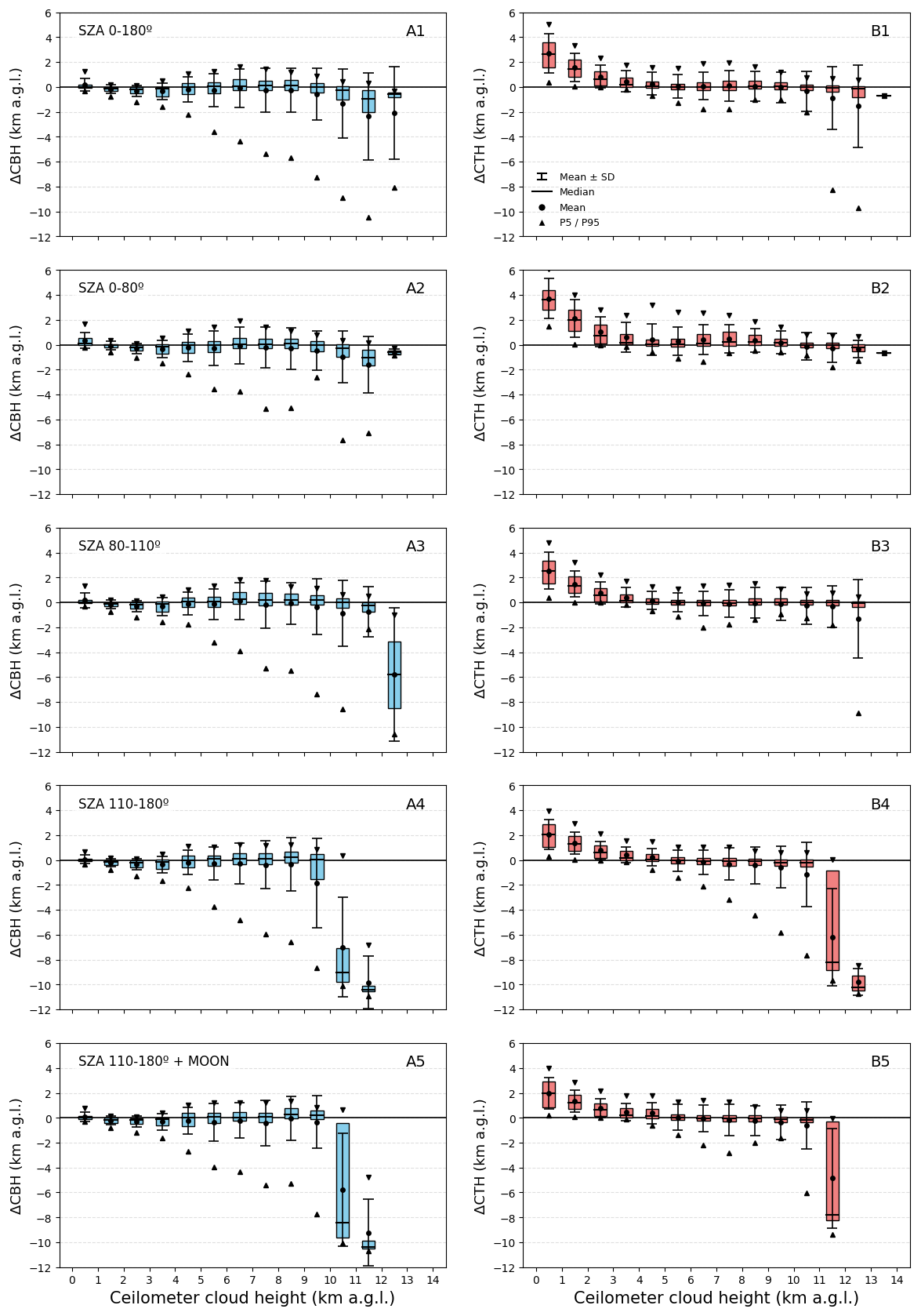
Figure 14 Box and whiskers plots for the differences between camera and ceilometer at 1 km height ceilometer cloud height bins. Camera values are based on the median height value within a 150 m radius of the ceilometer location. Filtering criteria have been applied to discard heights provided by less than two cameras, and those with fewer than 20 values and a standard deviation higher than 1 km. Column (A) Analysis for cloud base height (ΔCBH). Column (B) Analysis for cloud top height (ΔCTH). The boxes represent the interquartile range (IQR), the horizontal line is the median, and circular markers indicate the mean and triangle markers the percentiles (5th and 95th). Rows represent different lighting conditions: SZA 0–180° (all conditions), SZA 0–80° (daylight), SZA 80–110° (twilight), SZA 110–180° (night), and SZA 110–180° (night with moon presence).

Table 4 Statistical metrics including the number of coincident cloud height values (N), Mean Bias Error (MBE), Standard Deviation (SD), and Root Mean Square Error (RMSE), for the differences (ΔCBH and ΔCTH) between camera and ceilometer at 1 km ceilometer cloud height bins. Camera values are based on the median height value within a 150 m radius of the ceilometer location. Filtering criteria have been applied to discard heights provided by less than two cameras, and those with fewer than 20 values and a standard deviation higher than 1 km.

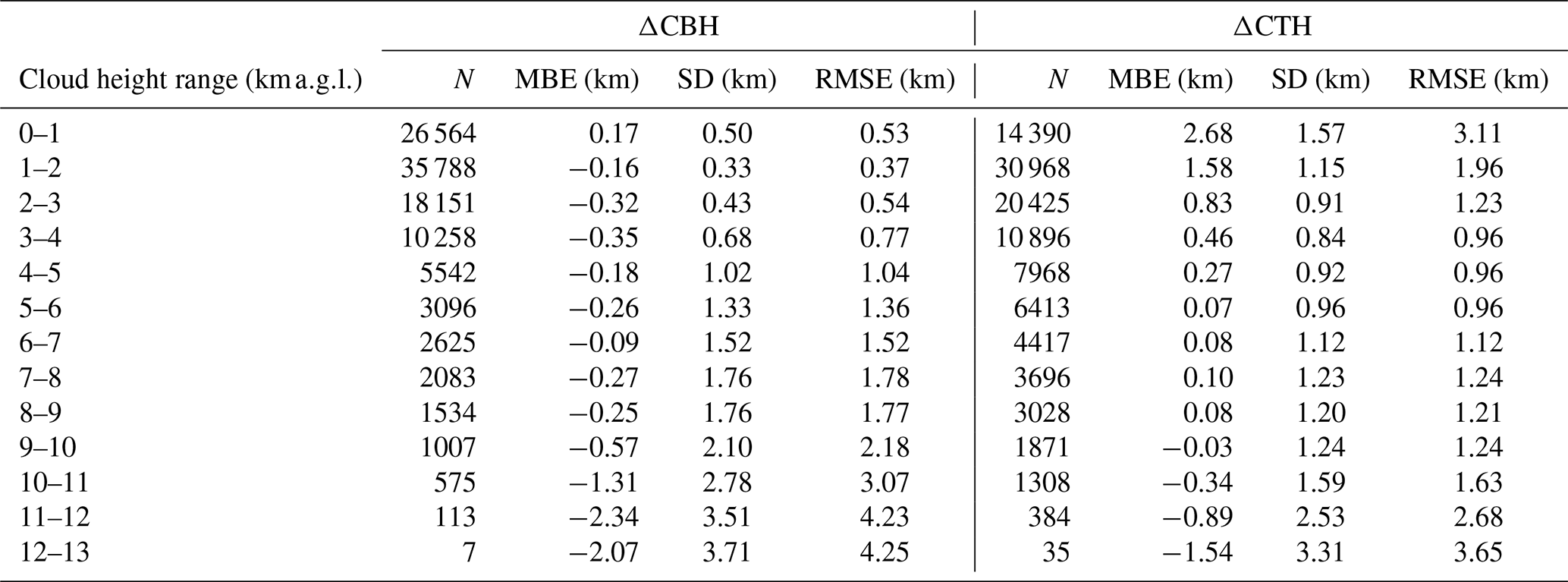
Regarding ΔCBH, for the all conditions case, both the mean and median values remain remarkably stable and near zero for cloud layers below 10 km. As indicated in Table 4, the MBE varies, from 0.17 km (0–1 km range) to −0.57 km (9–10 km range). However, for altitudes exceeding 10 km, there is a more significant underestimation of the CBH, with the MBE reaching −2.34 km in the 11–12 km interval. Figure 14A1–A5 reveals that this high altitude underestimation is primarily driven by nocturnal conditions, particularly during moonless nights (Panel A4), as expected, since high clouds, such as cirrus, are notably difficult to identify due to their high transparency. However, the retrieval of lower cloud layers (below 4–5 km) remains consistent regardless of lunar illumination. This is likely due to the reflection of artificial light from the city on the cloud base, providing sufficient contrast for the cameras to detect these lower layers even on moonless nights. In contrast, daytime observations (Panel A2) do not exhibit such dependence on altitude, showing only a slight underestimation. The dispersion of ΔCBH generally increases with cloud height. This is evidenced by the increase of IQR, a decrease in the P5, and a monotonic increase in the SD from 0.33 km at 1–2 to 3.71 km at the 12–13 km range. Notably, the higher SD in the 0–1 km range (0.50 km) compared to the 1–2 km range (0.33 km) likely reflects the initial lack of nearby cameras by the ceilometer location, until the installation of C030, enabling the retrieval of lower clouds from this point. These results suggest that while CBH retrieval is highly accurate and precise under daylight, precision decreases with altitude during low light conditions, with accuracy significantly degrading above 10 km.

The analysis for CTH, shows that the median of ΔCTH remains close to zero for most height ranges, except for the lowest layers (up to 3 km). For higher cloud heights, the mean values deviate from zero as well at nighttime conditions. However, the data availability for this high altitude clouds is considerably lower (see N in Table 4). In contrast, the results for low altitude clouds are highly representative, as they correspond to the height ranges with the largest number of observations. In these low layers, the cameras overestimate the ceilometer's CTH values, with MBE values ranging from 2.68 km (0–1 km range) to 0.83 km (2–3 km range). This overestimation is more pronounced during daytime conditions (Panel B2), which explains the poorer CTH agreement found for the daylight interval in Fig. 12. While the potential limitations causing this bias have been addressed previously, it is important to emphasize that the ceilometer's signal often fails to penetrate optically dense low clouds, preventing the detection of higher layers. This is likely to happen more during daylight hours, when solar background radiation increases the noise in the ceilometer signal and reduces its sensitivity to higher altitudes. Consequently, the cameras, which benefit from multiple viewing angles, may be obtaining in some cases true cloud tops that the ceilometer cannot resolve due to signal extinction. Regarding the precision of the CTH retrievals, although IQR exhibits larger values for clouds below 3 km, the SD remains relatively stable for mid level clouds (3–6 km), showing values around 1 km. The P5 values remain closer to zero for CTH than for CBH across most intervals, revealing a lower presence of extreme outliers in the cloud top estimates, except during moonless nights. These results indicate that the camera network is capable of retrieving the CTH with high accuracy and consistency for altitudes above 3 km.

In order to complement the statistical analysis, a direct comparison of two distinct days with varying cloud layer configurations is presented in Fig. 15. It illustrates the temporal evolution of the RCS (panels A and C) obtained by the ceilometer, and the estimated CBH and CTH from the camera network and the ceilometer (panels B and D). Consistent with the previous analysis, camera values are derived from the median height within a 150 m radius of the ceilometer's location.

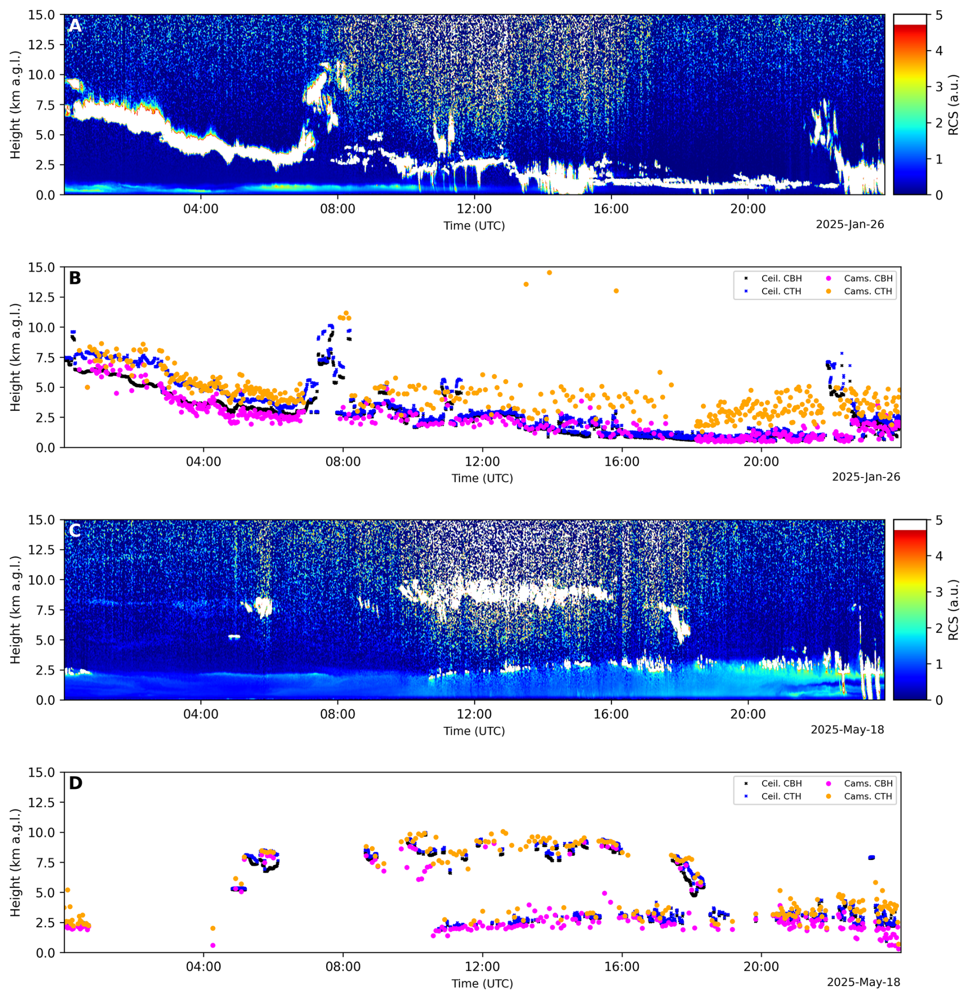
Figure 15 Temporal evolution for two different days of the ceilometer range corrected signal (RCS) overlaid with the cloud base and top heights (CBH and CTH) and those estimated by the all-sky camera network. Camera values are based on the median height value within a 150 m radius of the ceilometer location.

For the case of 26 January 2025, the RCS (panel A) shows the evolution of a day where a high to mid level cloud layer during the night gradually descended in altitude. At 07:00 UTC, another mid to high cloud is observed, and until 16:00 UTC, the RCS indicates the likely presence of a very low and thick cloud layer, as the ceilometer signal became saturated. Between 14:00–16:00 UTC, precipitation was likely occurring. In the afternoon, again a thick low level cloud layer appeared to saturate the RCS and at night, around 22:00–23:00 UTC, a higher cloud descended with precipitation. Regarding the CBH and CTH values in Panel B, clouds were detected by the ceilometer around 00:00 UTC about 10 km, that the cameras do not detect; as explained previously, this is likely because thin and translucent high clouds are extremely difficult to identify at night. During the rest of the night, both the CBH and CTH from the cameras show good agreement with the ceilometer. In the twilight intervals (around 07:00 and 18:00 UTC), the cameras show a lack of sensitivity, evidenced by two gaps in the cameras retrieved CBH and CTH. During daylight hours, the discrepancy in the cameras' CTH is likely partly due to the ceilometer signal saturating, whereas the cameras provide more information by viewing from different angles. Nevertheless, these values are also noisy. Also, during intervals with rain, droplet deposition on the domes, may explain the presence of high CTH outliers.

In the case of 18 May 2025, the RCS (Panel C) shows clouds around 2.5 km during the first hours of the night, followed by a cloud-free period. Around 05:00 UTC, higher clouds are seen at approximately 7.5 km. During the day, there was a more complex situation with a low layer at around 2.5 km that was probably not very opaque, allowing another layer to be detected between 7.5–10 km. From 18:00 UTC onward, only the lower layer remained. Regarding the cloud heights in Panel D, both instruments agree throughout the day, showing the capability of the cameras network to detect different cloud layers.

Finally, to evaluate the broader capabilities of the proposed method, based on the cameras network, an additional comparison has been performed using a second ceilometer situated at the Research Center for the Lower Atmosphere (CIBA), 35 km away from the primary site. This location also hosts an all-sky camera (C031, see Table 1). It is important to note that, due to the geometric limitations of the cameras' fields of view caused by the geographical camera distribution, and the criteria imposed in the proposed methodology, only high altitude clouds can be detected in this location. Figure 16 shows the camera CBH and CTH values against the ceilometer ones at CIBA station. This figure (panels A and B) clearly illustrates the mentioned limitation to high altitude layers, as no cloud retrievals are found below 7 km. Given this specific limitation, a categorical evaluation of cloud detection is not representative for this station. Camera values agree with the ceilometer cloud heights for both CBH and CTH values even for the low number of observations (CIBA's ceilometer was installed on 30 October 2025). Outliers where the cameras report high altitude clouds while the ceilometer identifies clouds at significantly lower levels (below 2 km) can be attributed to the presence of low clouds at CIBA that attenuate the ceilometer signal, preventing the detection of higher layers, as discussed previously. These outliers impact the accuracy and precision metrics of the dataset. The MBE is shifted toward overestimation, reaching 0.99 km for CBH and 1.19 km for CTH. Similarly, the precision is affected, with SD values of 2.40 and 2.65 km for CBH and CTH, respectively. Despite the presence of these outliers, it can be observed that the most frequent differences between the cameras and the ceilometer are centered around zero for both CBH and CTH. Nevertheless, if these specific outliers are discarded, the remaining data points align closely with the 1:1 line, demonstrating that the camera network is capable of providing reliable cloud height estimates even at significant distances from the network center.

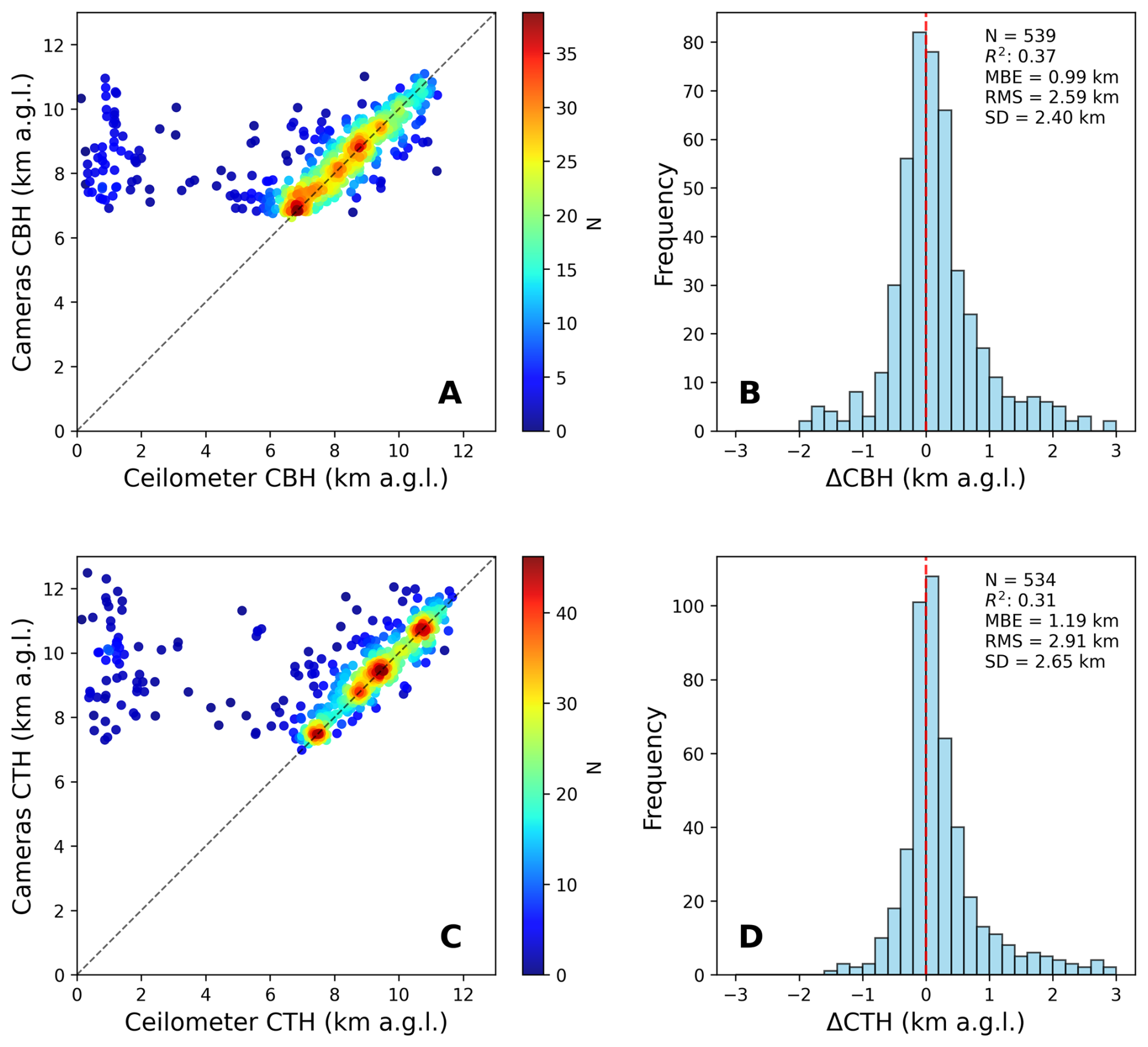
Figure 16 Bidimensional frequency histogram of median cloud heights values from the camera network within a 150 m radius of the CIBA ceilometer location, against ceilometer values for cloud base height (CBH) and cloud top height (CTH) in panels (A) and (C), respectively. Panels (B) and (D) represent the frequency histogram of the differences (ΔCBH and ΔCTH) between both instruments. Filtering criteria have been applied to discard heights provided by two or fewer cameras, with fewer than 20 height values and a standard deviation higher than 1 km. Results include total number of cases (N), coefficient of determination (R²), mean bias error (MBE), root mean square error (RMSE) and standard deviation (SD).

5 Conclusions

This work proposes a robust methodology for the identification and three dimensional localization of clouds using stereoscopic calculations, implemented through an unprecedented 20 all-sky camera dense network deployed around the city of Valladolid (Spain). It presents a novel aggregation strategy in which each camera is paired with every overlapping camera, and the resulting heights are combined onto a common spatial grid, together with a fully automated, near real time operational implementation, generating openly available cloud height products every 5 min during daytime and, as a further novelty, every 2 min at nighttime. The workflow also brings together for the first time a combination of different recommendations from previous studies, such as downsizing images, using rectified row-oriented pairs of simultaneous images to improve finding pixel correlations, using blocks of neighboring pixels in the correlation to avoid mismatches, using different baseline distances and applying smoothing filters that improve the segmentation of clouds. In addition, this implementation is also relevant due to the simultaneous application of all these novelties and aggregation strategies, while significantly optimizing the processes to achieve a high computational efficiency. For the case study shown in Sect. 3 (28 December 2025 at 11:20 UTC), the total processing time to retrieve cloud heights for the 16 available camera pairings was 102 s using our server infrastructure. However, this processing time is significantly optimized in the operational version through parallelization. By executing 40 processes simultaneously, a total of 120 cases (captured between 07:30–17:25 UTC) were processed in just 6min44 s. This results in an effective average processing time of 3.37 s per case. This allows for the generation of cloud position maps, including cloud base and top height (CBH and CTH), in near-real time, representing a substantial improvement over previous implementations.

The wide dispersion of the network enables the retrieval of a wide range of cloud heights, effectively reaching high clouds and providing observations from distant geographic positions. Potential biases are minimized by selecting for each case only those camera pairs that offer significant overlap for specific height ranges. A fundamental aspect of this methodology is its robust filtering process, which utilizes different criteria based on defining cloud levels and frequency analysis to validate the cloud height retrievals from the multiple camera pairs. These thresholds were selected empirically from a set of representative reference cases, balancing the rejection of outliers against the retention of a sufficient number of valid retrievals. This filtering stage is essential for integrating the vast amount of data generated by the network, as it successfully discards unrealistic values and allows for the determination of both CBH and CTH values.

Validation against a significantly larger dataset of ceilometer observations than those used in previous literature confirms that the network consistently detects clouds across a wide range of conditions. The proposed method is capable of obtaining the CBH with an accuracy, given by the mean bias error (MBE), of −0.14 km and a precision, reflected by the standard deviation (SD) of 0.78 km. In general, precision decreases with cloud height, and accuracy deteriorates for clouds above 10 km, especially during low light conditions such as night and twilight, corresponding to solar zenith angles (SZA) greater than 80°. This degraded performance at high cloud heights may be partly attributed to the presence of dirt or dust but also internal reflections over the camera domes, which can generate artifacts mistaken for low clouds. Furthermore, high clouds are more difficult to observe in low light situations, where the segmentation model also exhibits its poorest performance.

In addition, the proposed methodology is capable of estimating the CTH with considerable accuracy for clouds between 3–11 km, with MBE values ranging from 0.46 to −0.34 km, although it tends to overestimate the height of low clouds. This overestimation might not be entirely real, potentially resulting from the ceilometer's limited sensitivity to higher cloud layers when low level clouds are present. Under daytime conditions, the proposed method predicts the presence of clouds in 86 % of the cases identified by the reference instrument. This percentage decreases significantly at night to 62 % regardless of lunar illumination, and reaches its lowest point during twilight at 55 %. This lower identification rate is primarily due to the reduced performance of the segmentation model in these conditions. Additionally, longer exposure times at night result in increased image noise and sometimes in motion blur. This negatively affects the correlation between pixel blocks during the matching process.

The reliability of the system has been further corroborated through comparison with a second ceilometer located more than 35 km away from the center of the network. This analysis confirms that the method accurately identifies CBH and CTH even in locations distant from the densest part of the network, with the most frequent differences falling within the −0.2–0.2 km range. However, due to geometric limitations, the minimum detectable cloud height increases with distance from the network; thus, lower clouds are only detectable near the cameras, while the detection area for high clouds is significantly larger.

This methodology provides not only vertical resolution but also high spatial resolution (0.0005° ∼50 m), producing cloud masks similar to those obtained by satellites. A case study comparison with Sentinel-2 revealed that the methodology effectively captures the spatial distribution of clouds, with discrepancies mainly found at cloud edges due to temporal mismatches or specific filtering thresholds. These results highlight the potential of the PRESENTE network for satellite calibration and validation tasks with a high spatial and temporal resolution even in near-real time.

Although this study focused on CBH and CTH, with the aforementioned limitations, the developed methodology has the potential to reconstruct full 3D cloud structures, which can be explored in future work. This is particularly valuable for cloud modeling and monitoring in near-real time. Also, for studying cloud interactions with other atmospheric components such as aerosols or solar and thermal radiation. The adaptability of the methodology, including the ability to increase temporal resolution as needed or to be applied to other scaled cameras network, establishes it as a powerful and flexible tool for atmospheric research.

To ensure the generation of high quality products, several critical factors must be meticulously managed, including the maintenance of clean camera domes to prevent the appearance of artifacts, the precise synchronization of internal clocks to ensure simultaneous image acquisition, and the implementation of geometric calibrations that are both reliable and frequently updated to account for even minor positional changes. Looking ahead, the methodology could be further improved by establishing dynamic filtering thresholds tailored to cloud height and the number of available images, as well as by developing an advanced segmentation model capable of more effectively distinguishing between clear sky and clouds, with a specific focus on high clouds during both daytime and challenging low-light conditions such as nighttime or during sunrise and sunset.