On the origin of the twilight color index maximum and its application to cloud-height retrieval

A number of previous studies have demonstrated the capability of detecting high-altitude clouds during twilight using the color index (CI), defined as the ratio of zenith intensities at two different wavelengths, typically selected in the visible range or near infrared (NIR). When high clouds are present, a maximum or minimum (depending on the wavelengths selection) is observed in the CI signal (Sarkissian et al., 1991; Toledo et al., 2016). These studies also showed that the solar zenith angle (SZA) at which the CI maximum or minimum occurs (SZA_max) strongly depends on cloud altitude, enabling cloud-height retrieval through comparison with radiative transfer (RT) simulations. Twilight conditions require RT simulations in spherical geometry, which are computationally expensive. In this work, it is introduced a single-scattering formulation of the CI that provides a physically transparent framework for identifying the mechanisms that determine the SZA of the CI maximum and, consequently, the inferred cloud altitude. The simplified formulation is explicitly compared with Monte Carlo RT simulations in spherical geometry and is shown to accurately reproduce the behavior of SZA_max over a wide range of conditions relevant for high-altitude clouds. In particular, the model provides reliable cloud-height estimates for cloud optical depths up to τ_C≲0.3. Within this single-scattering formulation, it is demonstrated that SZA_max occurs at the SZA for which the relative SZA-variations of the zenith intensity at the two selected wavelengths become equal, thereby explaining the emergence of the extremum in differential terms. However, achieving a well-defined CI extremum requires selecting two wavelengths with sufficient spectral separation, typically spanning distinct regions of the visible–NIR spectrum. To overcome this spectral dependence, it is introduced a Rayleigh-referenced color index (CI^R), defined as the ratio between the measured zenith intensity and the corresponding intensity expected for a purely Rayleigh-scattering atmosphere at the same wavelength. This index reproduces the characteristic extrema associated with high-altitude clouds while requiring simulations and observations at only a single wavelength. The proposed formulation facilitates extensive sensitivity studies and provides greater flexibility in spectral selection, particularly in regions affected by gas absorption.

1 Introduction

Clouds play a major role in Earth's climate system through their influence on the planetary radiation budget (Ramanathan et al., 1989). High-altitude clouds such as cirrus clouds, which cover a large fraction of Earth’s surface (∼30 %), are especially important because they interact with both incoming solar and outgoing terrestrial radiation (Hartmann et al., 2001). In the visible range, cirrus clouds scatter part of the incident solar radiation back to space (the albedo effect), while in the infrared they absorb and re-emit terrestrial radiation, contributing to the greenhouse effect. As a result, their overall climatic impact depends strongly on their optical and microphysical properties. Monitoring cirrus clouds through remote sensing observations is therefore essential for characterizing their spatial and temporal variability and for improving their representation in climate models. In addition, since cirrus clouds typically form in the upper troposphere close to the tropopause, determining their altitude can also provide a useful lower bound for the tropopause height.

In addition to cirrus clouds in the upper troposphere, other types of high-altitude clouds also play an important role in atmospheric processes. For instance, polar stratospheric clouds (PSCs), which form in the stratosphere during the cold polar winter, are particularly important because they participate in chemical reactions that lead to ozone depletion. PSCs are composed of supercooled ternary solutions (STS), nitric acid trihydrate (NAT), and/or ice particles (Spang et al., 2018), which provide surfaces for heterogeneous reactions that release reactive chlorine and bromine species that subsequently participate in catalytic ozone destruction cycles. Monitoring PSCs using remote sensing techniques is therefore essential for understanding their composition, microphysics, and variability, as well as for assessing their impact on stratospheric chemistry and ozone layer evolution.

Among the different techniques available for the observation of high-altitude clouds, lidar instruments provide some of the most detailed measurements. Both ground-based and spaceborne lidars, such as the Cloud-Aerosol Lidar with Orthogonal Polarization (CALIOP) (Winker et al., 2009) on board the Cloud-Aerosol Lidar and Infrared Pathfinder Satellite Observations (CALIPSO) satellite, allow the detection of clouds and the retrieval of their vertical structure with high vertical resolution. However, the number of ground-based lidar stations is relatively limited and their geographical coverage remains sparse. For this reason, complementary observational techniques have been developed to investigate high-altitude clouds. Although these techniques generally provide less detailed information about cloud microphysical properties, they can offer valuable insights into their occurrence and variability. In this context, Sarkissian et al. (1991) proposed the use of ground-based UV-VIS spectroscopic observations to detect PSCs and estimate their altitudes during twilight through the analysis of the color index (CI), defined as the ratio between intensities measured at two different wavelengths. This approach was later extended to the detection of cirrus and subvisual cirrus clouds using ground-based optical measurements based on the CI derived from dual-channel radiometric observations (Toledo et al., 2016).

The objective of this work is to investigate the physical basis that explains why the CI can be effectively used for the detection and characterization of high-altitude clouds during twilight. To this end, a new formulation based on the single-scattering approximation is introduced. In addition, methodological improvements are investigated in order to enhance the robustness and applicability of this technique. This study is motivated by recent works in which the CI approach has also been applied to ground-based zenith DOAS observations (Gomez-Martin et al., 2021; Lauster et al., 2022), further demonstrating the potential of twilight measurements for the study of high-altitude aerosol layers. The paper is organized as follows. Section 2 introduces the CI technique and describes how it can be used during twilight for the detection of high-altitude clouds and the estimation of their altitudes. Section 3 presents the new methodology developed in this work to investigate the influence of clouds on the CI signal, as well as an alternative index based on measurements at a single wavelength. Section 4 presents a series of sensitivity analyses, and Sect. 5 summarizes the main conclusions of this study.

2 The color index approach

The detection and characterization of clouds can be achieved by monitoring the evolution of the CI during twilight. In this work, twilight is defined as the time period when the solar zenith angle (SZA) ranges between 90 and 100°. For a given SZA, the CI is defined as:

$$\begin{array}{}\text{(1)}& \text{CI}\left(\text{SZA}\right)={\displaystyle \frac{I({\mathit{\lambda }}_{\mathrm{2}},\text{SZA})}{I({\mathit{\lambda }}_{\mathrm{1}},\text{SZA})}},\end{array}$$

where I represents the intensity at zenith at the wavelengths λ₁ and λ₂, generally selected in the visible or near-infrared range. The presence of high-altitude clouds induces a maximum or a minimum in the CI signal, depending on the choice of λ₁ and λ₂. The SZA at which this maximum or minimum occurs (SZA_max) depends on the cloud altitude. To simplify notation, subsequent references to the maximum or minimum in the CI signal will be denoted as CI_max. On Earth, CI_max primarily arises from the wavelength dependence of molecular opacity (Rayleigh scattering), as demonstrated in Sect. 3.1. In the absence of a significant spectral variation of the background atmospheric opacity between the two wavelengths, no pronounced maximum or minimum would be expected in the CI signal. Although this approach for cloud-altitude characterization is straightforward, it relies on three-dimensional RT simulations in spherical geometry (as SZA>90°), whose computational cost for a given cloud, aerosol scenario, and wavelength is very high. Furthermore, the geometry of the problem implies that the cloud layer cannot be modeled as a spherical shell in RT simulations at twilight (Gomez-Martin et al., 2021; Lauster et al., 2022). Assuming that the cloud under study is the only cloud present in the atmospheric scene, treating it as a spherical shell rather than as a localized layer would imply that, for SZA>90°, the direct solar radiation interacts twice with the cloud (see Fig. 1). This would imply a cloud layer extending horizontally over several hundred kilometers, which is not realistic and could lead to simulations that do not accurately represent actual atmospheric conditions. For these reasons, in the next section it is analyzed the CI under the single-scattering approximation, introducing a new methodology that provides a clearer understanding of the factors driving the maximum in the CI when high-altitude clouds are present. The goal of this approach is not only to reduce the computational complexity and facilitate the exploration of different atmospheric scenarios, but also to enable a more transparent investigation of the physical processes governing CI_max.

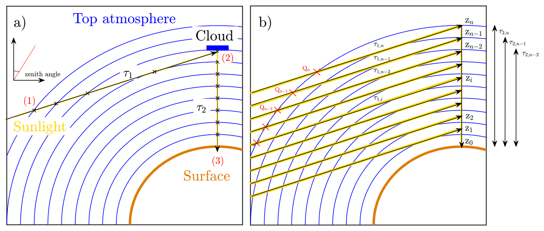
Figure 1 (a) Schematic showing the path followed by a direct solar photon scattered by a cloud at a scattering angle equal to the SZA. The inset illustrates the definition of the zenith angle. Direct light enters the atmosphere at point (1) and propagates to point (2), where it is scattered by the cloud toward the instrument located at point (3). The quantities τ₁ and τ₂ represent the opacity due to molecules and aerosols along segments (1)–(2) and (2)–(3), respectively. (b) Same as panel (a), but for trajectories intersecting the vertical axis at point (3) at different altitudes (z₁,z₂, …,z_n). The points Q_n, Q_n−1, … indicate the locations where direct solar radiation enters the atmosphere for the different trajectories.

3 Single scattering color index

3.1 Methodology

Instead of solving the RT equation under the single-scattering approximation, it is formulated the problem in terms of the probability that an instrument located at the surface and pointing at the zenith detects a photon scattered by a cloud at an altitude h_C during twilight. If it is assumed that photons undergo at most a single scattering event, then for given values of SZA, h_C, and λ, the probability P that the instrument detects a cloud-scattered photon can be written as:

$$\begin{array}{}\text{(2)}& \begin{array}{rl}P(\text{SZA},z=h_{\mathrm{C}},\mathit{\lambda })& =P_{\mathrm{1}}(\text{SZA},z=h_{\mathrm{C}},\mathit{\lambda })\\ & \times P_{\mathrm{2}}^{\mathrm{c}}(\text{SZA},z=h_{\mathrm{C}},\mathit{\lambda })\\ & \times P_{\mathrm{3}}(\text{SZA},z=h_{\mathrm{C}},\mathit{\lambda })\end{array}\end{array}$$

Here, (i) P₁ represents the probability that a direct solar photon reaches the cloud without being scattered or absorbed along its trajectory from the top of the atmosphere to the cloud (path between points (1) and (2) in Fig. 1a); (ii) $P_{\mathrm{2}}^{\mathrm{c}}$ represents the probability that the cloud scatters the photon toward the instrument, corresponding to a scattering angle equal to the SZA; and (iii) P₃ is the probability that a photon at altitude h_C, traveling downward at a zenith angle of 180°, reaches the instrument without undergoing absorption or additional scattering (path between points (2) and (3) in Fig. 1a). The probabilities P₁ and P₃ are determined by the properties of the background atmosphere at wavelength λ, whereas $P_{\mathrm{2}}^{\mathrm{c}}$ depends solely on the cloud scattering optical depth and phase function. Equation (2) accounts only for photons scattered by the cloud at altitude h_C. Therefore, to reproduce the total zenith intensity measured at the surface, contributions from photons scattered at all altitudes and by molecules or other aerosols present in the atmosphere must be considered. In this case, the total probability of detecting a photon with the instrument (P_Total) is obtained by integrating P over altitude (see the right panel of Fig. 1b):

$$\begin{array}{}\text{(3)}& \begin{array}{r}{P}_{\mathrm{Total}}(\mathit{\lambda },\mathrm{SZA})\\ & =\underset{z_{\mathrm{dark}}}{\overset{z_{\mathrm{top}}}{\int }}{P}_{\mathrm{1}}(z,\mathit{\lambda },\mathrm{SZA})\\ & \times P_{\mathrm{2}}(z,\mathit{\lambda },\mathrm{SZA})\times P_{\mathrm{3}}(z,\mathit{\lambda })\mathrm{d}z,\end{array}\end{array}$$

where P₂ represents the probability that a photon is scattered at altitude z into the zenith line of sight of the instrument, corresponding to a scattering angle θ=SZA with respect to the incident solar direction. Note that in Eq. (3), P₂ evaluated at z=h_C accounts for photons scattered by the cloud, molecules, and any other aerosols present at that altitude. If the molecular and aerosol opacities are negligible at h_C, then $P_{\mathrm{2}}\left(h_{\mathrm{C}}\right)=P_{\mathrm{2}}^{\mathrm{c}}\left(h_{\mathrm{C}}\right)$. Here, z_top denotes the altitude of the top of the atmosphere, while z_dark, which depends on the SZA, denotes the lowest altitude that still receives direct solar illumination during twilight. Below z_dark, direct solar radiation is completely blocked by the Earth's curvature. From Eq. (3), it is defined the single-scattering CI as:

$$\begin{array}{}\text{(4)}& {\mathrm{CI}}^{\ast }\left(\mathrm{SZA}\right)={\displaystyle \frac{P_{\mathrm{Total}}({\mathit{\lambda }}_{\mathrm{2}},\mathrm{SZA})}{P_{\mathrm{Total}}({\mathit{\lambda }}_{\mathrm{1}},\mathrm{SZA})}},\end{array}$$

where λ₂>λ₁. To compute P_Total, explicit expressions for P₁, P₂, and P₃ are required. For a given altitude z above the instrument and a given SZA, the probability P₁ can be written as

$$\begin{array}{}\text{(5)}& P_{\mathrm{1}}(z,\mathit{\lambda },\mathrm{SZA})=\exp \left[-{\mathit{\tau }}_{\mathrm{1}}(z,\mathrm{SZA},\mathit{\lambda })\right],\end{array}$$

where ${\mathit{\tau }}_{\mathrm{1}}(z,\mathrm{SZA},\mathit{\lambda })$ is the optical depth along the line of sight (see Fig. 1). To estimate ${\mathit{\tau }}_{\mathrm{1}}(z,\mathrm{SZA},\mathit{\lambda })$, it is assumed that aerosol and molecular extinction (S) decrease exponentially with altitude, with scale heights H^A and H^M, respectively:

$$\begin{array}{}\text{(6)}& \begin{array}{rl}{\displaystyle }S(z,\mathit{\lambda })& {\displaystyle }=S_{\mathrm{0}}^{\mathrm{A}}\left(\mathit{\lambda }\right)\exp \left(-{\displaystyle \frac{z}{H^{\mathrm{A}}}}\right)+S_{\mathrm{0}}^{\mathrm{M}}\left(\mathit{\lambda }\right)\exp \left(-{\displaystyle \frac{z}{H^{\mathrm{M}}}}\right)\\ {\displaystyle }& {\displaystyle }={\displaystyle \frac{{\mathit{\tau }}_{\mathrm{0}}^{\mathrm{A}}\left(\mathit{\lambda }\right)}{H^{\mathrm{A}}}}\exp \left(-{\displaystyle \frac{z}{H^{\mathrm{A}}}}\right)+{\displaystyle \frac{{\mathit{\tau }}_{\mathrm{0}}^{\mathrm{M}}\left(\mathit{\lambda }\right)}{H^{\mathrm{M}}}}\exp \left(-{\displaystyle \frac{z}{H^{\mathrm{M}}}}\right),\end{array}\end{array}$$

where $S_{\mathrm{0}}^{\mathrm{A}}$ and $S_{\mathrm{0}}^{\mathrm{M}}$ are the aerosol and molecular extinction coefficients at the surface, and ${\mathit{\tau }}_{\mathrm{0}}^{\mathrm{A}}$ and ${\mathit{\tau }}_{\mathrm{0}}^{\mathrm{M}}$ are the corresponding total aerosol and molecular optical depths. For a given altitude z above the instrument and a given SZA, the optical depth along the line of sight is given by

$$\begin{array}{}\text{(7)}& \begin{array}{rl}{\displaystyle }& {\displaystyle }{\mathit{\tau }}_{\mathrm{1}}(z,\mathrm{SZA},\mathit{\lambda })=S_{\mathrm{0}}^{\mathrm{A}}\left(\mathit{\lambda }\right){\int }_{\mathrm{0}}^{l(z,\mathrm{SZA})}\\ {\displaystyle }& {\displaystyle }\exp \left[-{\displaystyle \frac{\sqrt{{l^{\prime }}^{\mathrm{2}}+(R_{\mathrm{T}}+z{)}^{\mathrm{2}}+\mathrm{2}{l}^{\prime }\mathit{\mu }(R_{\mathrm{T}}+z)}-R_{\mathrm{T}}}{H^{\mathrm{A}}}}\right]\mathrm{d}{l}^{\prime }\\ {\displaystyle }& {\displaystyle }+S_{\mathrm{0}}^{\mathrm{M}}\left(\mathit{\lambda }\right){\int }_{\mathrm{0}}^{l(z,\mathrm{SZA})}\\ {\displaystyle }& {\displaystyle }\exp \left[-{\displaystyle \frac{\sqrt{{l^{\prime }}^{\mathrm{2}}+(R_{\mathrm{T}}+z{)}^{\mathrm{2}}+\mathrm{2}{l}^{\prime }\mathit{\mu }(R_{\mathrm{T}}+z)}-R_{\mathrm{T}}}{H^{\mathrm{M}}}}\right]\mathrm{d}{l}^{\prime },\end{array}\end{array}$$

where l(z,SZA) is the distance between the point (0,z) and the intersection with the top of the atmosphere (points Q_i in Fig. 1b). To derive Eq. (7), it is used the relation $r=\sqrt{l^{\mathrm{2}}+(R_{\mathrm{T}}+z{)}^{\mathrm{2}}+\mathrm{2}l\mathit{\mu }(R_{\mathrm{T}}+z)}$, where r is the radial distance, R_T is the planetary radius, and μ=cos (SZA). Using trigonometry, the path length l(z,SZA) can be expressed as a function of z and the SZA:

$$\begin{array}{}\text{(8)}& \begin{array}{rl}l(z,\mathrm{SZA})& =\sqrt{(z_{\mathrm{top}}+R_{\mathrm{T}}{)}^{\mathrm{2}}+(z+R_{\mathrm{T}}{)}^{\mathrm{2}}\left[{\sin }^{\mathrm{4}}\left(\mathit{\alpha }\right)\right.}\\ & \stackrel{\mathrm{‾}}{\left.-{\cos }^{\mathrm{4}}\left(\mathit{\alpha }\right)\right]+\mathrm{2}(z+R_{\mathrm{T}})\sin \left(\mathit{\alpha }\right)}\\ & \stackrel{\mathrm{‾}}{\sqrt{(z_{\mathrm{top}}+R_{\mathrm{T}}{)}^{\mathrm{2}}-(z+R_{\mathrm{T}}{)}^{\mathrm{2}}{\cos }^{\mathrm{2}}\left(\mathit{\alpha }\right)}},\end{array}\end{array}$$

where $\mathit{\alpha }=\mathrm{SZA}-\mathrm{90}$°. It is important to note that, for the estimation of τ₁, the opacity of the cloud is not included. This is because, in our model, the cloud has a limited horizontal extent and is localized above the instrument, rather than being treated as a spherical shell. The treatment of the cloud horizontal extent, and its impact on P₁, is introduced later in the context of the comparison with the Monte Carlo simulations.

The integrals in Eq. (7) do not admit analytical solutions and must therefore be evaluated numerically. Since the terms $S_{\mathrm{0}}^{\mathrm{A}}$ and $S_{\mathrm{0}}^{\mathrm{M}}$ are outside the integrals, a precomputed look-up table for the integrals in Eq. (7) as a function of z, SZA, H^A, and H^M can be constructed. In this case, P₁ can be written as

$$\begin{array}{}\text{(9)}& \begin{array}{rl}{P}_{\mathrm{1}}(z,\mathrm{SZA},\mathit{\lambda })& =\exp \left[-\left(J^{\mathrm{A}}(z,\mathrm{SZA},H^{\mathrm{A}})S_{\mathrm{0}}^{\mathrm{A}}\left(\mathit{\lambda }\right)\right.\right.\\ & \left.\left.+J^{\mathrm{M}}(z,\mathrm{SZA},H^{\mathrm{M}})S_{\mathrm{0}}^{\mathrm{M}}\left(\mathit{\lambda }\right)\right)\right],\end{array}\end{array}$$

where J^A and J^M denote the integrals in Eq. (7), which are precomputed and therefore do not need to be recalculated when the wavelength or the aerosol scenario is changed.

As indicated above, P₂ represents the probability that direct solar radiation reaching an altitude z above the instrument is scattered at a scattering angle equal to the SZA. Consequently, this probability is proportional to the scattering extinction coefficient at altitude z – including contributions from aerosols, molecules, and clouds – and to the phase function p(θ) evaluated at θ=SZA. If the vertical distribution of the cloud is described by a Gaussian height profile, then P₂ can be written as:

$$\begin{array}{}\text{(10)}& \begin{array}{rl}{\displaystyle }{P}_{\mathrm{2}}& {\displaystyle }(z,\mathrm{SZA},\mathit{\lambda })=C\left[S_{\mathrm{0}}^{\mathrm{A}}\right(\mathit{\lambda }\left){\mathit{\omega }}^{\mathrm{A}}\right(\mathit{\lambda }\left)\exp \left(-{\displaystyle \frac{z}{H^{\mathrm{A}}}}\right)p^{\mathrm{A}}\right(\mathit{\lambda },\mathrm{SZA})\\ {\displaystyle }& {\displaystyle }+S_{\mathrm{0}}^{\mathrm{M}}\left(\mathit{\lambda }\right){\mathit{\omega }}^{\mathrm{M}}\left(\mathit{\lambda }\right)\exp \left(-{\displaystyle \frac{z}{H^{\mathrm{M}}}}\right)p^{\mathrm{M}}(\mathit{\lambda },\mathrm{SZA})\\ {\displaystyle }& {\displaystyle }+{\displaystyle \frac{{\mathit{\tau }}^{\mathrm{C}}\left(\mathit{\lambda }\right){\mathit{\omega }}^{\mathrm{C}}\left(\mathit{\lambda }\right)}{\mathrm{\Delta }{h}_{\mathrm{C}}}}\sqrt{{\displaystyle \frac{\mathrm{2}}{\mathit{\pi }}}}\exp \left[-{\displaystyle \frac{\mathrm{2}(z-h_{\mathrm{C}}{)}^{\mathrm{2}}}{\mathrm{\Delta }{h}_{\mathrm{C}}^{\mathrm{2}}}}\right]p^{\mathrm{C}}(\mathit{\lambda },\mathrm{SZA})],\end{array}\end{array}$$

where ω^A, ω^M, and ω^C are the aerosol, molecular, and cloud single-scattering albedos, respectively; p^A, p^M, and p^C are the corresponding phase functions; τ^C and Δh_C are the cloud total optical depth and geometrical thickness; and C is a normalization constant that, as shown below, does not need to be explicitly evaluated in our analysis. In Eq. (10), the only term depending explicitly on the SZA is the phase function. However, given the limited SZA range considered here, the impact of phase-function variations on SZA_max is expected to be small.

The last term to be computed is P₃(z,λ), which represents the probability that a photon travels vertically from altitude z to the surface without undergoing absorption or scattering. This probability is given by

$$\begin{array}{}\text{(11)}& P_{\mathrm{3}}(z,\mathit{\lambda })=\exp \left[-{\mathit{\tau }}_{\mathrm{2}}(z,\mathit{\lambda })\right],\end{array}$$

where τ₂(z,λ) is the optical depth due to aerosols, molecules, and clouds between altitude z and the surface (see Fig. 1), and is computed as

$$\begin{array}{}\text{(12)}& \begin{array}{rl}{\displaystyle }{\mathit{\tau }}_{\mathrm{2}}(z,\mathit{\lambda })& {\displaystyle }={\mathit{\tau }}_{\mathrm{0}}^{\mathrm{A}}\left(\mathrm{1}-\exp \left[-{\displaystyle \frac{z}{H^{\mathrm{A}}}}\right]\right)+{\mathit{\tau }}_{\mathrm{0}}^{\mathrm{M}}\left(\mathrm{1}-\exp \left[-{\displaystyle \frac{z}{H^{\mathrm{M}}}}\right]\right)\\ {\displaystyle }& {\displaystyle }+{\displaystyle \frac{{\mathit{\tau }}_{\mathrm{C}}}{\mathrm{2}}}\left[\mathtt{\text{erf}}\left(\sqrt{\mathrm{2}}{\displaystyle \frac{z-h_{\mathrm{C}}}{\mathrm{\Delta }{h}_{\mathrm{C}}}}\right)-\mathtt{\text{erf}}\left(-\sqrt{\mathrm{2}}{\displaystyle \frac{h_{\mathrm{C}}}{\mathrm{\Delta }{h}_{\mathrm{C}}}}\right)\right].\end{array}\end{array}$$

Here, erf denotes the error function, defined as

$$\begin{array}{}\text{(13)}& \mathtt{\text{erf}}\left(x\right)={\displaystyle \frac{\mathrm{2}}{\sqrt{\mathit{\pi }}}}\underset{\mathrm{0}}{\overset{x}{\int }}{e}^{-t^{\mathrm{2}}}\mathrm{d}t.\end{array}$$

Once P₁, P₂, and P₃ are defined, the total probability P_Total is obtained by integrating their product from z_dark to the top of the atmosphere. Scripts to compute P₁, P₂, P₃, and P_Total are publicly available at Toledo (2026).

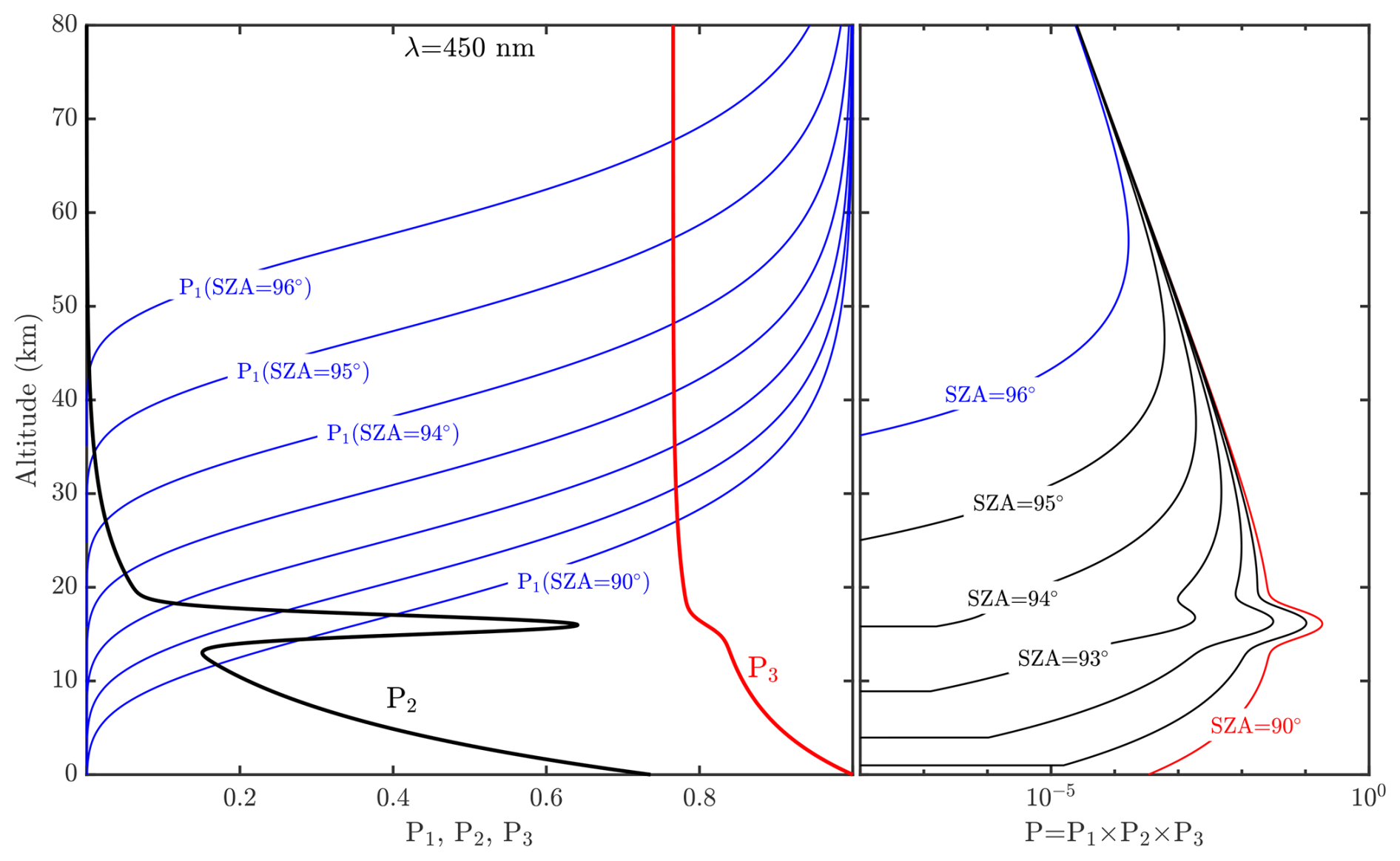
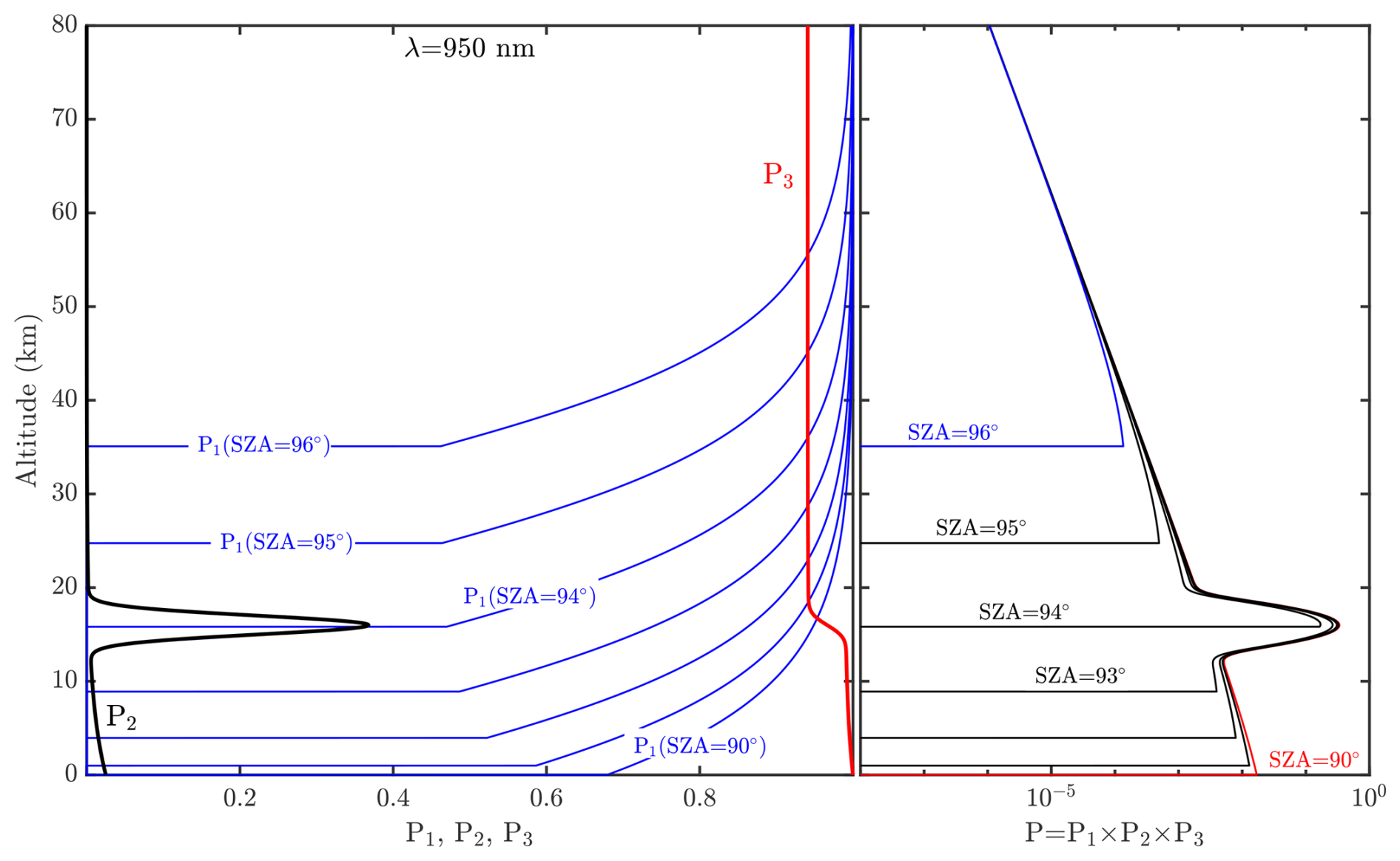
Figure 2 Variation of P₁, P₂, P₃, and P with altitude at 450 nm for different SZAs (90, 91, 92, 93, 94, 95, and 96°), considering a cloud layer located at an altitude of 16 km, with a geometrical thickness of 2 km and a total optical depth of 0.05. The P₂ curves (left panel) were normalized by P_Total at SZA=90°.

In the following sections, it is first analyzed the behavior of P₁, P₂, and P₃, and their contribution to P_Total, in order to study the properties of the CI as a function of cloud altitude and wavelengths. It is shown that the single-scattering CI^∗ reproduces the main features of the CI obtained from full Monte Carlo RT simulations.

3.2 Simulation of P₁, P₂, P₃, P_Total and CI^*

Figures 2 and 3 show the variation of P₁, P₂, P₃, and P with altitude at 450 and 950 nm for different SZAs, considering a cloud layer located at an altitude of 16 km. In these simulations, the phase functions were omitted in the computation of P₂, and both ω^M and ω^C were set to unity. The P₂ curves were normalized by P_Total at SZA=90°. As discussed below, for a given cloud scenario, the choice of normalization in Eq. (10) does not affect the value of SZA_max derived from the model. As shown in Figs. 2 and 3, P₁ increases with altitude and decreases with SZA as a consequence of the dependence of τ₁ (Eq. 7) on these parameters. For a given altitude z above the surface, the path segment between points Q and (0,z) intersects progressively lower atmospheric layers as the SZA increases, where the molecular opacity is higher, leading to larger values of τ₁. For fixed values of SZA and z, P₁ is also larger at 950 nm than at 450 nm, reflecting the decrease of Rayleigh opacity with increasing wavelength. At 450 nm (Fig. 2) and for SZA≳93°, most of the photons reaching the instrument originate from scattering events occurring at altitudes above the cloud layer, as indicated by the behavior of P in Fig. 2. The altitude at which direct solar radiation is completely blocked by the Earth curvature is given by

$$\begin{array}{}\text{(14)}& z_{\mathrm{dark}}=R_{\mathrm{T}}\left(\sqrt{\mathrm{1}+{\tan }^{\mathrm{2}}\left(\mathit{\alpha }\right)}-\mathrm{1}\right),\end{array}$$

Thus, for SZA=93 and 94°, z_dark is 8.7 and 15.5 km, respectively, which are both below the altitude of maximum cloud opacity (h_C=16 km). This indicates that, at 450 nm, and as a result of molecular opacity, the cloud is already effectively in darkness before the surface blocks direct solar radiation at the cloud altitude (SZA>94°). In contrast, at 950 nm (Fig. 3) , and for z_dark<h_C, the maximum in P occurs at the cloud altitude (for SZA=93 and 94°). Therefore, depending on the wavelength, the cloud can enter the dark region of the atmosphere even when h_C>z_dark. As discussed below, this behavior is one of the primary factors responsible for the emergence of a maximum in the CI in the presence of high-altitude clouds. With regard to P₂ and P₃, larger values of P₂ are obtained at 450 nm than at 950 nm as a consequence of the stronger molecular opacity at shorter wavelengths. However, since P₁ decreases much more rapidly at 450 nm than at 950 nm for altitudes above z_dark, and because P₃ is larger at 950 nm than at 450 nm, the resulting values of P are greater at 950 nm for altitudes near the cloud layer (i.e., for z>z_dark).

Figure 3 Same as Fig. 2, but at 950 nm.

These results are further illustrated in Fig. 4a, where the P profiles at 450 and 950 nm are compared for three different SZA values. The horizontal black dashed lines indicate the altitude z_dark corresponding to each SZA. When SZA∼90°, the dominant contribution of photons at both wavelengths originates from altitudes around the cloud layer. However, as the SZA increases, the contribution from these altitudes decreases more rapidly at 450 nm than at 950 nm. As a result, P_Total decreases more slowly with increasing SZA at 950 nm than at 450 nm, and it is precisely this effect that causes CI^∗ to increase over this SZA range, as shown in Fig. 4b. The increase in CI^∗ continues up to SZA∼93.8°, beyond which CI^∗ decreases rapidly with SZA. By comparing the P profiles with the CI^∗ signal in Fig. 4, it is seen that this transition occurs close to the moment when the cloud begins to darken at 950 nm. These results indicate that the maximum in CI^∗ occurs at larger SZA values as λ₂ increases, since lower molecular opacity delays the onset of cloud darkening. In the limiting case where the molecular opacity at λ₂ is negligible, SZA_max approaches SZA_dark, which can be obtained from Eq. (14) by setting z=h_C. For the example shown in Fig. 4, SZA_dark=94.06°, which is close to the corresponding value of SZA_max. From this, it is concluded that for a given SZA_max, the cloud altitude must satisfy

$$\begin{array}{}\text{(15)}& h_{\mathrm{C}}\ge R_{\mathrm{T}}\left(\sqrt{\mathrm{1}+{\tan }^{\mathrm{2}}({\mathrm{SZA}}_{\max }-{\mathrm{90}}^{\circ })}-\mathrm{1}\right).\end{array}$$

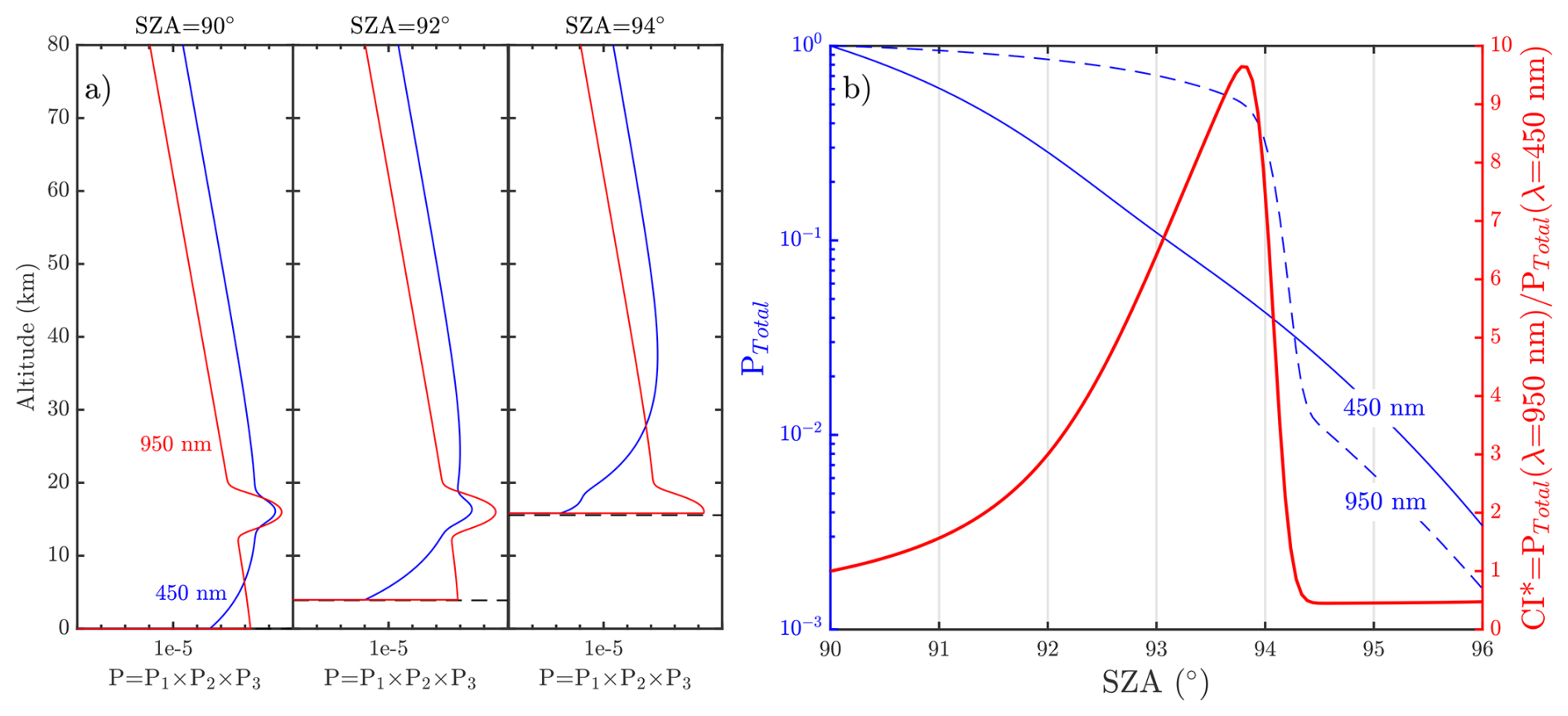
Figure 4 (a) Vertical profiles of P at 450 nm (blue lines) and 950 nm (red lines) for SZA=90, 92, and 94°. The atmospheric scenario is the same as in Figs. 2 and 3. (b) Variation of P_Total at 450 nm (blue solid line) and 950 nm (blue dashed line) with SZA for the atmospheric conditions of Figs. 2 and 3. The red solid line represents CI^∗ obtained from P_Total at 450 and 950 nm.

If an increase in λ₂ results in an increase in the value of SZA_max, the next point to address is the dependence of SZA_max on λ₁ for a fixed λ₂. It was performed simulations similar to those shown in Fig. 4 for different values of λ₁ and found almost no variation in SZA_max when λ₁ ranges between 400 and 500 nm while λ₂ is fixed at 950 nm. Although the shape of the CI^∗ signal changes, the value of SZA_max remains nearly unchanged. However, for larger values of λ₁, a noticeable shift in SZA_max is observed. In the following section, it is further investigated how variations in λ₁ influence CI_max.

3.3 Origin of the wavelength dependence of the CI^∗ maximum

To study the dependence of SZA_max on λ₁ and λ₂ for a given cloud scenario, the condition defining the maximum of CI^∗ is examined. This condition is obtained by differentiating the ratio defined in Eq. (4) with respect to the SZA and setting the derivative equal to zero. Under this condition, SZA_max satisfies:

$$\begin{array}{}\text{(16)}& \begin{array}{rl}& {\displaystyle \frac{\mathrm{1}}{P_{\mathrm{Total}}({\mathit{\lambda }}_{\mathrm{1}},\mathrm{SZA})}}{\displaystyle \frac{\partial P_{\mathrm{Total}}({\mathit{\lambda }}_{\mathrm{1}},\mathrm{SZA})}{\partial \mathrm{SZA}}}\\ & ={\displaystyle \frac{\mathrm{1}}{P_{\mathrm{Total}}({\mathit{\lambda }}_{\mathrm{2}},\mathrm{SZA})}}{\displaystyle \frac{\partial P_{\mathrm{Total}}({\mathit{\lambda }}_{\mathrm{2}},\mathrm{SZA})}{\partial \mathrm{SZA}}}\end{array}\end{array}$$

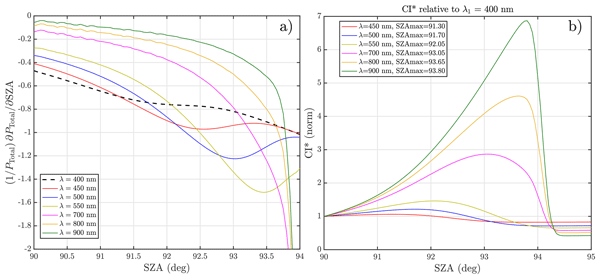
Equation (16) shows that the CI^∗ maximum occurs at the SZA for which both wavelengths exhibit identical relative SZA-variations of P_Total. In other words, the maximum does not arise only from the cloud contribution, but from the differential evolution of the zenith intensity with SZA at the two selected wavelengths. Equation (16) also indicates that any multiplicative constant applied to P_Total in Eq. (3), such as a normalization factor, does not modify the value of SZA_max.

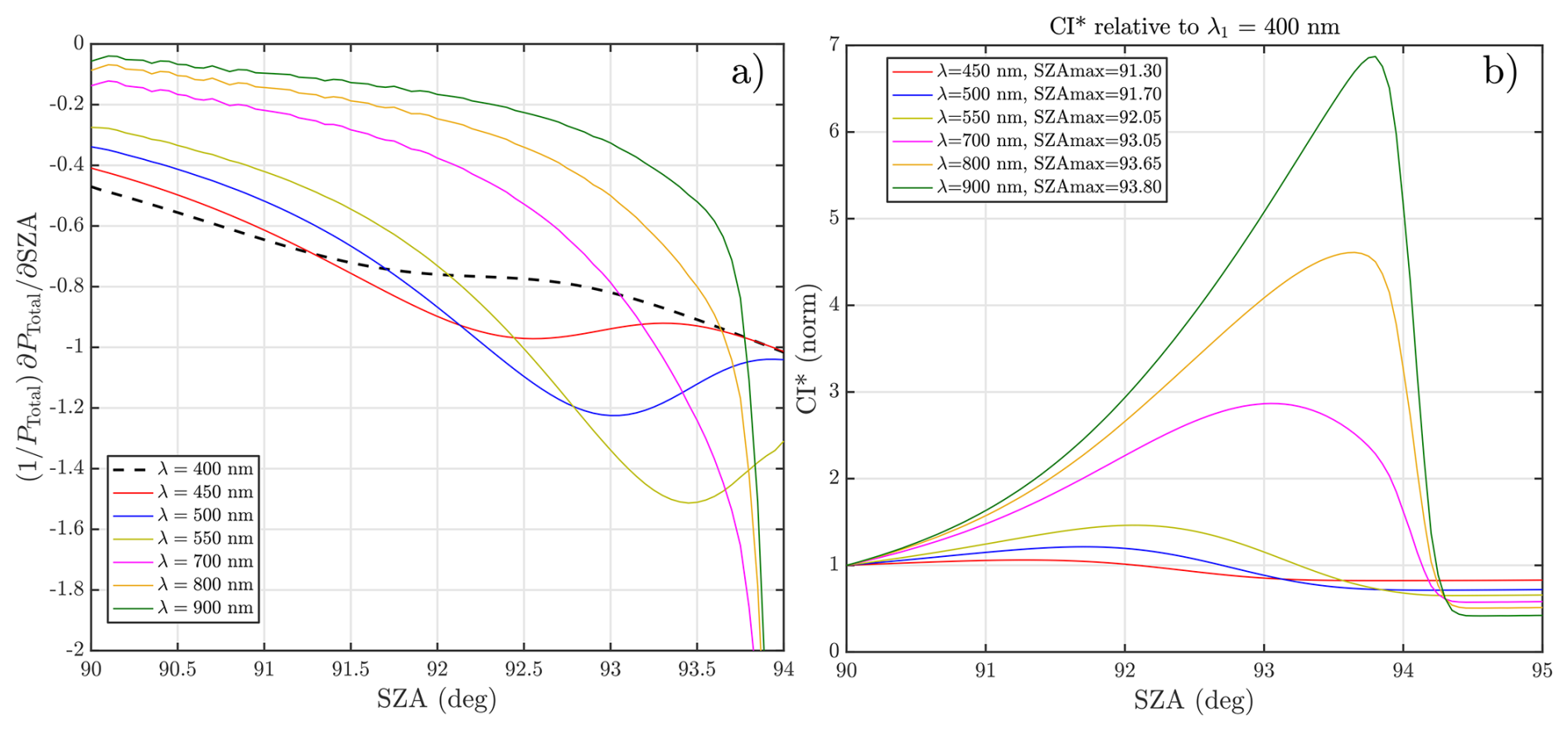
As an example, Fig. 5a shows the relative rate of variation of P_Total(λ,SZA) with respect to SZA at different wavelengths for the same cloud scenario as in Figs. 2 and 3. Figure 5b shows the corresponding CI^∗ signals for the same cloud scenario and wavelength combinations as in Fig. 5a, with λ₁=400 nm fixed and λ₂ varying. The results at 600 and 650 nm have been omitted for clarity, as they follow the smooth spectral evolution observed between the neighbouring wavelengths (550 and 700 nm) and therefore do not provide additional qualitative information. As expected, SZA_max coincides with the SZA at which the relative SZA-variation curves of P_Total intersect. In the previous section, it was indicated that simulations similar to those shown in Fig. 4, but considering λ₁ values between 400 and 500 nm while keeping λ₂=950 nm fixed, exhibit no significant variations in SZA_max. This behaviour is readily understood from the relative SZA-variation curves of P_Total, where the curves corresponding to 400 and 500 nm are nearly indistinguishable for SZA≳93.5°. As a result, their intersection with the λ₂=950 nm curve occurs at essentially the same SZA, leading to nearly identical values of SZA_max. However, if instead of using λ₂=950 nm it is considered λ₂≲700 nm, noticeable variations in SZA_max may arise when λ₁ is varied between 400 and 500 nm.

Figure 5a also shows that, as λ₂ increases relative to 400 nm, the intersection between the corresponding relative SZA-variation curves becomes progressively more transversal, which corresponds to a larger difference between their local slopes at the crossing point. As a consequence, the curvature of CI^∗ around SZA_max increases, leading to a more pronounced and better-defined maximum in Fig. 5b. Conversely, when the relative variation curves intersect with nearly parallel slopes, the resulting CI^∗ maximum is broader and less pronounced. This aspect is particularly relevant for real zenith radiance measurements, where instrumental noise and atmospheric variability introduce uncertainties in the determination of SZA_max. A sharper maximum enhances the robustness of cloud detection and improves the precision in the inferred cloud altitude.

Although these results suggest that increasing the spectral separation between λ₁ and λ₂ generally leads to a sharper CI^∗ maximum and therefore to potentially more precise determinations of SZA_max, the situation is more complex in practice. The shape of the relative SZA-variation curves of P_Total also depend on the cloud altitude and on the overall atmospheric optical properties. Consequently, identifying an optimal combination of λ₁ and λ₂ that minimizes the uncertainty in the retrieved cloud height is not straightforward. In the following section, it is introduced an alternative CI-based index specifically designed to improve the robustness of twilight cloud-height estimation.

Figure 5 Variation of $\left(\frac{\mathrm{1}}{P_{\text{Total}}(\mathit{\lambda },\text{SZA})}\cdot \frac{\partial P_{\text{Total}}(\mathit{\lambda },\text{SZA})}{\partial \text{SZA}}\right)$ with SZA at 400, 450, 500, 550, 700, 800 and 900 nm for the atmospheric conditions of Figs. 2 and 3. Panel (b) shows the corresponding CI^∗ signals for the same atmospheric conditions as in panel (a), with λ₁=400 nm fixed and λ₂=450, 500, 550, 700, 800, and 900 nm.

3.4 Spectral selection constraints and development of a Rayleigh-based CI

In the previous section, it was highlighted the difficulty of identifying a globally optimal combination of λ₁ and λ₂ even under the simplified assumption of a single cloud layer and molecular scattering only. In realistic atmospheric conditions, however, additional components such as aerosol layers or absorbing gases further increase the complexity of twilight RT. An example is the analysis of CI at wavelengths where the absorption of NO₂ or O₃ is significant (Gomez-Martin et al., 2021). In such cases, the presence of an absorbing layer modifies the total optical depth and therefore affects P_Total. Consequently, its contribution must be explicitly incorporated into the analysis. The absorption opacity due to gases can be directly included in Eqs. (7) and (12) if vertical profiles are available, or alternatively parametrized using a Gaussian profile similar to that adopted for the cloud layer. Assuming a Gaussian-type parametrization, the contribution to P₁ requires a term analogous to J^A and J^M, following the same procedure used in Eq. (7) but with a Gaussian dependence on z. For the calculation of P₃ through τ₂, the absorption opacity of gases (τ^Abs) can be incorporated into Eq. (12) through

$$\begin{array}{}\text{(17)}& \begin{array}{rl}& {\mathit{\tau }}^{\mathrm{Abs}}(z,\mathit{\lambda })={\displaystyle \frac{{\mathit{\tau }}_{\mathrm{Abs}}^{\mathrm{Total}}}{\mathrm{2}}}\left[\mathrm{erf}\left(\sqrt{\mathrm{2}}{\displaystyle \frac{z-h_{\mathrm{Abs}}}{\mathrm{\Delta }{h}_{\mathrm{Abs}}}}\right)\right.\\ & \left.-\mathrm{erf}\left(-\sqrt{\mathrm{2}}{\displaystyle \frac{h_{\mathrm{Abs}}}{\mathrm{\Delta }{h}_{\mathrm{Abs}}}}\right)\right],\end{array}\end{array}$$

where ${\mathit{\tau }}_{\mathrm{Abs}}^{\mathrm{Total}}$, h_Abs, and Δh_Abs denote the total optical depth, central altitude, and geometrical thickness of the absorbing layer, respectively.

However, in many cases these gases exhibit a pronounced seasonal variability in both their vertical distribution and total column abundance (see, e.g., Gomez-Martin et al., 2021), and an inaccurate representation of such temporal cycles may lead to significant errors in the retrieved cloud altitude. To illustrate this point, we performed a series of sensitivity tests considering a Gaussian absorbing layer centred at 20 km, with a geometrical thickness of 10 km, and a total absorption optical depth ranging from 0.01 to 0.1 at λ₁=400 nm, while assuming negligible gaseous absorption at λ₂. These calculations were not intended to reproduce a particular atmospheric absorber, but rather to provide a generic test case for investigating the influence of gaseous absorption on CI-based cloud-height retrievals. The simulations show that the displacement of SZA_max generally increases as the spectral separation between the two wavelengths decreases. For example, for a cloud located at 18 km and an absorption optical depth of 0.05, the maximum displacement reached approximately 0.43° for the $\mathrm{400}/\mathrm{500}$ nm wavelength pair, corresponding to an error of about 2 km in the retrieved cloud height. This value should not be regarded as universal, since the impact depends on the selected wavelengths, the cloud altitude, and the optical depth and vertical distribution of the absorbing species. To mitigate these modelling uncertainties, one possible approach is to select λ₁ and λ₂ outside the main absorption bands of the gases present, thereby simplifying the RT modelling.

However, this criterion – avoiding absorption bands while simultaneously maximizing the spectral separation between λ₁ and λ₂ in order to enhance the robustness of the retrieval – is not always feasible in practice. Figure 6 illustrates this limitation by showing, as representative examples, the absorption cross sections of NO₂ (green) and O₃ (blue), derived from Burrows et al. (1998) and Molina and Molina (1986). The spectral bands selected in previous CI-based retrieval studies are also indicated for reference. Figure 5 shows that a suitable choice for λ₁ is around 400 nm, since the cloud signature at this wavelength is less pronounced than at longer wavelengths, which leads to a more pronounced CI^∗ maximum. Figure 6 shows that selecting λ₁ in the blue spectral region is problematic due to the significant absorption of NO₂ in this range. Although one could shift λ₁ towards 500–550 nm to reduce this effect, such a displacement would require a corresponding shift in λ₂ in order to preserve sufficient spectral separation. This would extend the required spectral range beyond the capabilities of many instruments. For instance, Gomez-Martin et al. (2021) employed measurements from a twin (UV/Vis) Multi-Axis Differential Optical Absorption Spectroscopy (MAX-DOAS) system covering the spectral range from 415 to 542 nm, which limits the available wavelength combinations for CI-based retrievals. It is important to note that the absorbers shown in Fig. 6 are representative of the atmospheric conditions considered in Gomez-Martin et al. (2021). Under different atmospheric conditions, other absorbers, such as H₂O, may also need to be taken into account if their vertical distribution extends sufficiently high to influence the CI-based retrievals.

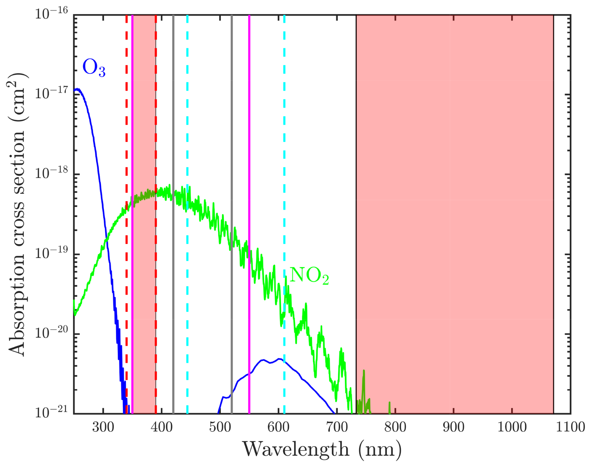
Figure 6 Absorption cross sections of NO₂ (green) and O₃ (blue) from Burrows et al. (1998) and Molina and Molina (1986), respectively. The gray and purple solid vertical lines indicate the wavelength pairs selected by Gomez-Martin et al. (2021) and Sarkissian et al. (1991), respectively, for the computation of the CI. The red and cyan dashed vertical lines indicate the wavelength pairs adopted by Lauster et al. (2022) for the UV and visible CI, respectively. The red shaded regions represent the wavelength ranges employed by Toledo et al. (2016).

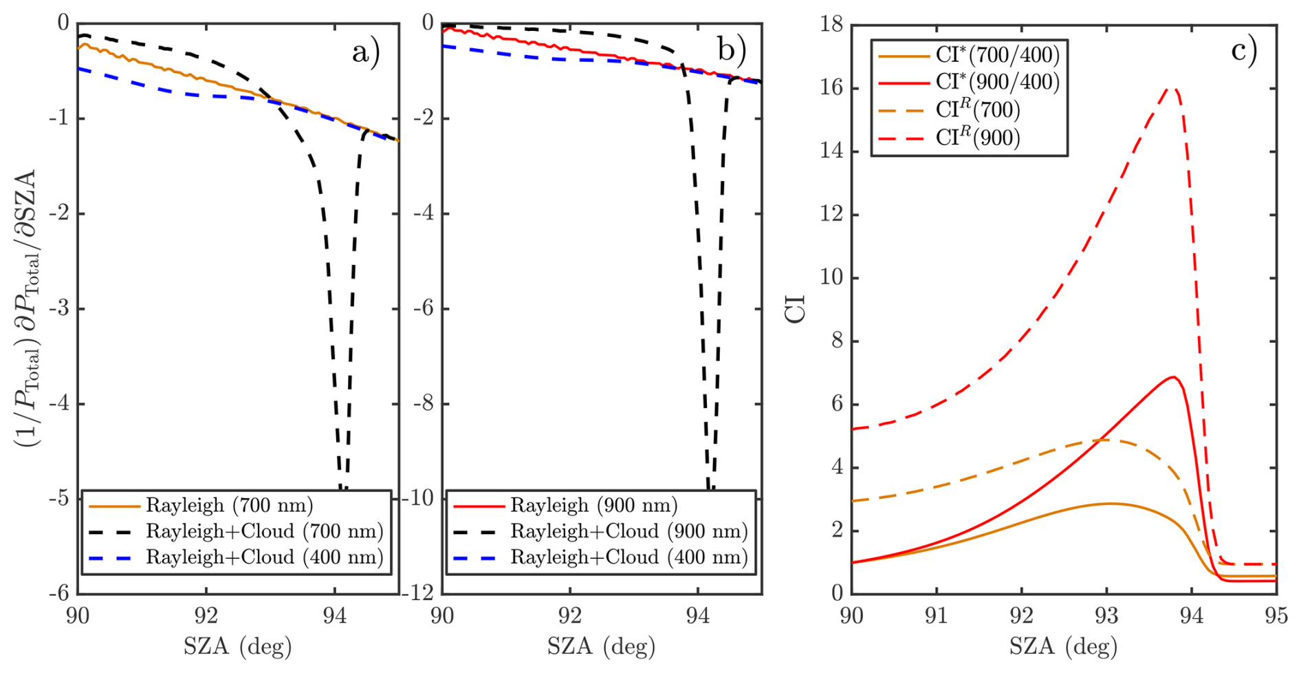
Figure 7 (a) Variation of $\left(\frac{\mathrm{1}}{P_{\text{Total}}(\mathit{\lambda },\text{SZA})}\cdot \frac{\partial P_{\text{Total}}(\mathit{\lambda },\text{SZA})}{\partial \text{SZA}}\right)$ with SZA for a purely Rayleigh atmosphere at 700 nm, and for an atmosphere including Rayleigh scattering and a cloud layer at 16 km (as in Fig. 5) at 400 and 700 nm. Panel (b) shows the same comparison as panel (a), but for 900 nm instead of 700 nm. Panel (c) compares CI^∗ and CI^R for the same cloud scenario as in panels (a) and (b). For CI^∗, λ₁=400 nm and λ₂=700 and 900 nm are used, while CI^R is computed at λ=700 and 900 nm.

The objective of this section is to define a new CI formulation that enables the detection of clouds during twilight and the estimation of their altitude, while avoiding the need to select λ₁ in spectral regions that are problematic for RT simulations. As shown in Figs. 2 and 6, when λ₁=400 nm (or similar) is employed, the CI^∗ maximum occurs at an SZA at which the cloud is already completely in shadow. Thus, at λ₁ and for SZA values around or larger than SZA_max, P_Total does not differ significantly from that expected in a purely Rayleigh-scattering atmosphere. Indeed, Fig. 7a and b show the relative SZA-variation curves $\frac{\mathrm{1}}{P_{\mathrm{Total}}(\mathit{\lambda },\mathrm{SZA})}\frac{\partial P_{\mathrm{Total}}(\mathit{\lambda },\mathrm{SZA})}{\partial \mathrm{SZA}}$ for both the cloud + Rayleigh scenario and the pure Rayleigh case at 400, 700, and 900 nm. In these cases, it can be seen that the relative variations in the pure Rayleigh atmosphere closely resemble those of the cloud + Rayleigh case at 400 nm in the vicinity of the intersection of the curves that determines SZA_max. From this reasoning, it is defined a Rayleigh-referenced color index, CI^R, as

$$\begin{array}{}\text{(18)}& {\mathrm{CI}}^{\mathrm{R}}\left(\mathrm{SZA}\right)={\displaystyle \frac{P_{\mathrm{Total}}(\mathit{\lambda },\mathrm{SZA})}{P_{\mathrm{Total}}^{\mathrm{R}}(\mathit{\lambda },\mathrm{SZA})}},\end{array}$$

where $P_{\mathrm{Total}}^{\mathrm{R}}(\mathit{\lambda },\mathrm{SZA})$ denotes the total signal simulated (or measured, if radiances are used) under purely Rayleigh-scattering conditions at wavelength λ. The principle of cloud detection using Eq. (18) is analogous to that of CI^∗, but with the advantage that it requires observations at only a single wavelength. This allows its application to instruments operating at a single wavelength (or within a narrow spectral band that does not permit the selection of two widely separated wavelengths), thereby simplifying the choice of spectral regions where the observations are less affected by gas absorption. Moreover, provided that the molecular scale height and background atmospheric composition remain stable over time, the SZA dependence of the twilight intensity at a given wavelength in a purely Rayleigh atmosphere is expected to be nearly invariant. Therefore, the same Rayleigh reference signal can be used for the calculation of CI. To show this, Fig. 7c illustrates CI^∗ computed for λ₁=400 nm and λ₂=700 and 900 nm, together with CI^R calculated at λ=700 and 900 nm for the same cloud scenario as in Fig. 5. These results clearly demonstrate that, despite being a considerably simpler index, CI^R effectively captures the presence of high-altitude clouds during twilight and enables their height to be estimated through RT simulations at a single wavelength.

3.5 Comparison against Monte-Carlo simulations

The analyses presented in the previous sections have allowed us to identify the key processes controlling the behaviour of the CI and have led to the definition of a new index, the Rayleigh-referenced color index, CI^R, which may offer practical advantages over the traditional CI based on measurements at two wavelengths. However, it remains necessary to assess how well the single-scattering formulation reproduces the results obtained from a multiple-scattering model in spherical geometry through a comparison of the simulated zenith intensity at twilight. For this purpose, a Monte Carlo RT model was employed, previously used to simulate twilight clouds on Earth (Toledo et al., 2016; Gomez-Martin et al., 2021), Mars (Toledo et al., 2023, 2024), and Titan (West et al., 2016). In order to improve the consistency of the comparison, the vertical and horizontal structure of the cloud is the same in both models. The cloud is assumed to follow a Gaussian distribution not only in the vertical, as described in Eq. (10), but also in the horizontal direction. In this formulation, the cloud extinction coefficient decreases with the horizontal distance from the observer zenith according to:

$$\begin{array}{}\text{(19)}& {\mathit{\beta }}^{\mathrm{C}}(z,\mathit{\rho },\mathit{\lambda })={\displaystyle \frac{{\mathit{\tau }}^{\mathrm{C}}\left(\mathit{\lambda }\right)}{\mathrm{\Delta }{h}_{\mathrm{C}}}}\sqrt{{\displaystyle \frac{\mathrm{2}}{\mathit{\pi }}}}\exp \left[-{\displaystyle \frac{\mathrm{2}(z-h_{\mathrm{C}}{)}^{\mathrm{2}}}{\mathrm{\Delta }{h}_{\mathrm{C}}^{\mathrm{2}}}}\right]\exp \left[-{\displaystyle \frac{{\mathit{\rho }}^{\mathrm{2}}}{\mathrm{2}{R}_{\mathrm{C}}^{\mathrm{2}}}}\right],\end{array}$$

where R_C defines the horizontal extent of the cloud and ρ is the horizontal distance from the local vertical axis of the observer. The horizontal distance is approximated as ρ(l)=r(l) ζ(l), where r(l) is the radial distance along the solar path and ζ(l) is the angular deviation from the local vertical. Here, l denotes the path length along the solar trajectory, as defined in Eq. (8). For clarity, the dependence of l on z and SZA has been omitted in the notation. The angular deviation ζ(l) is obtained from the spherical geometry of the solar path as:

$$\begin{array}{}\text{(20)}& \begin{array}{rl}\mathit{\zeta }\left(l\right)& =\arccos \left({\displaystyle \frac{R_T+z+l\cos \left(\mathrm{SZA}\right)}{r\left(l\right)}}\right)\\ & =\arccos \left({\displaystyle \frac{R_T+z+l\cos \left(\mathrm{SZA}\right)}{\sqrt{l^{\mathrm{2}}+(R_T+z{)}^{\mathrm{2}}+\mathrm{2}l\cos (\mathrm{SZA}\left)\right(R_T+z)}}}\right).\end{array}\end{array}$$

Note that both P₂ and P₃ are evaluated along the vertical direction of the observer (i.e., at ρ=0). As a result, the horizontal Gaussian distribution does not affect these terms, since the cloud extinction reaches its maximum along the symmetry axis. In contrast, the horizontal structure of the cloud directly impacts the computation of P₁, as the incoming solar radiation propagates along a slanted path and samples regions with ρ≠0. However, since this contribution enters as an additional extinction term, it can be naturally incorporated into the computation of P₁ by including it in the optical depth integral defined in Eq. (7):

$$\begin{array}{}\text{(21)}& \begin{array}{rl}{P}_{\mathrm{1}}(z,\mathrm{SZA},\mathit{\lambda })& =\exp \left[-\left(J^{\mathrm{A}}(z,\mathrm{SZA},H^{\mathrm{A}})S_{\mathrm{0}}^{\mathrm{A}}\left(\mathit{\lambda }\right)\right.\right.\\ & +J^{\mathrm{M}}(z,\mathrm{SZA},H^{\mathrm{M}})S_{\mathrm{0}}^{\mathrm{M}}\left(\mathit{\lambda }\right)\\ & \left.\left.+\underset{\mathrm{0}}{\overset{l(z,\mathrm{SZA})}{\int }}{\mathit{\beta }}^{\mathrm{C}}\left(z\right(l^{\prime }),\mathit{\rho }(l^{\prime }),\mathit{\lambda })\mathrm{d}{l}^{\prime }\right)\right],\end{array}\end{array}$$

Figures 8a–e show simulations of the variation of the normalized intensity with SZA obtained using the Monte Carlo RT model and the single-scattering approach described in Sect. 3.1, for a cloud layer with τ^C=0.05 and $h_{\mathrm{C}}=\mathrm{12},\mathrm{14},\mathrm{16},\mathrm{18}$ and 20 km. For all simulations, the wavelength was fixed at λ=700 nm, the horizontal scale at R_C=20 km, and the cloud thickness at Δh_C=2 km. The Monte Carlo simulations are limited to SZA=95° due to the increased computational cost associated with the adopted cloud geometry. In contrast to spherically symmetric cloud layers, the horizontally localized cloud considered here breaks the symmetry between SZA and latitude, requiring independent simulations for each SZA. This range nevertheless fully covers the region of interest, since the SZA_max for each simulated cloud height occurs at SZA below 95°, as indicated by the dashed black line.

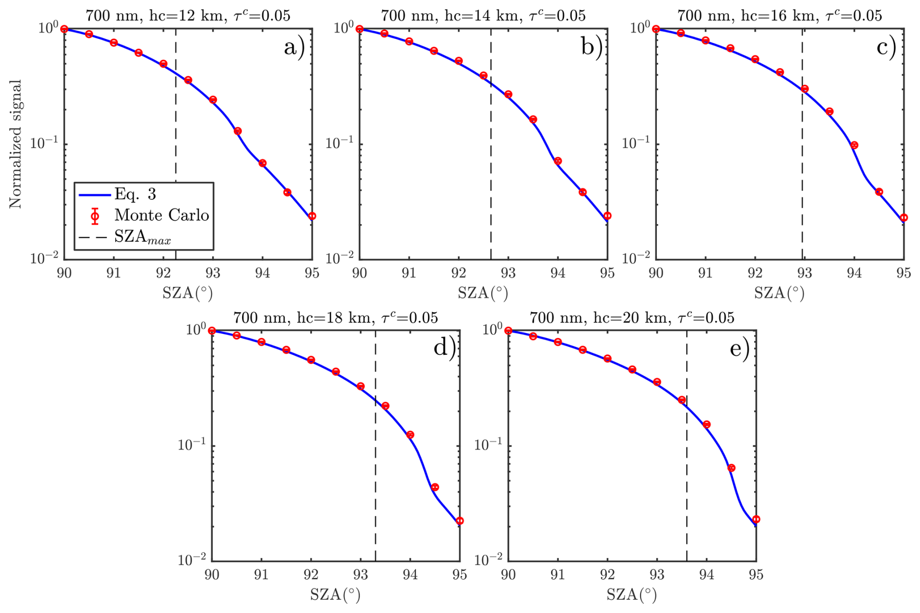
Figure 8 Normalized zenith intensity as a function of SZA for different cloud heights: h_C=12 km (a), 14 km (b), 16 km (c), 18 km (d), and 20 km (e). All simulations were performed at 700 nm, with cloud optical thickness τ_C=0.05, horizontal scale R_C=20 km, and cloud geometrical thickness Δh_C=2 km. Monte Carlo simulations are shown as red dots, while the single-scattering model is represented by the blue solid lines. The black dashed line indicates the value of SZA_max corresponding to each cloud scenario, assuming λ₁=400 nm.

The comparison shown in Fig. 8 demonstrates that the single-scattering model (hereafter SSM) reproduces the Monte Carlo simulations with very good agreement across the full range of cloud altitudes considered. Small differences between both approaches can be observed at larger SZAs (typically above ∼94°), where the deviations slightly increase. However, the SZAs relevant for the determination of the CI maximum occur at lower values, as indicated by the dashed black line marking SZA_max in each panel. Therefore, within the range of interest, the approximations adopted in the SSM remain well within acceptable limits. These results not only support the validity of the formulation developed in the previous sections for investigating the physical origin of the CI maximum, but also demonstrate that the SSM provides a reliable and computationally efficient alternative for the analysis of observational data.

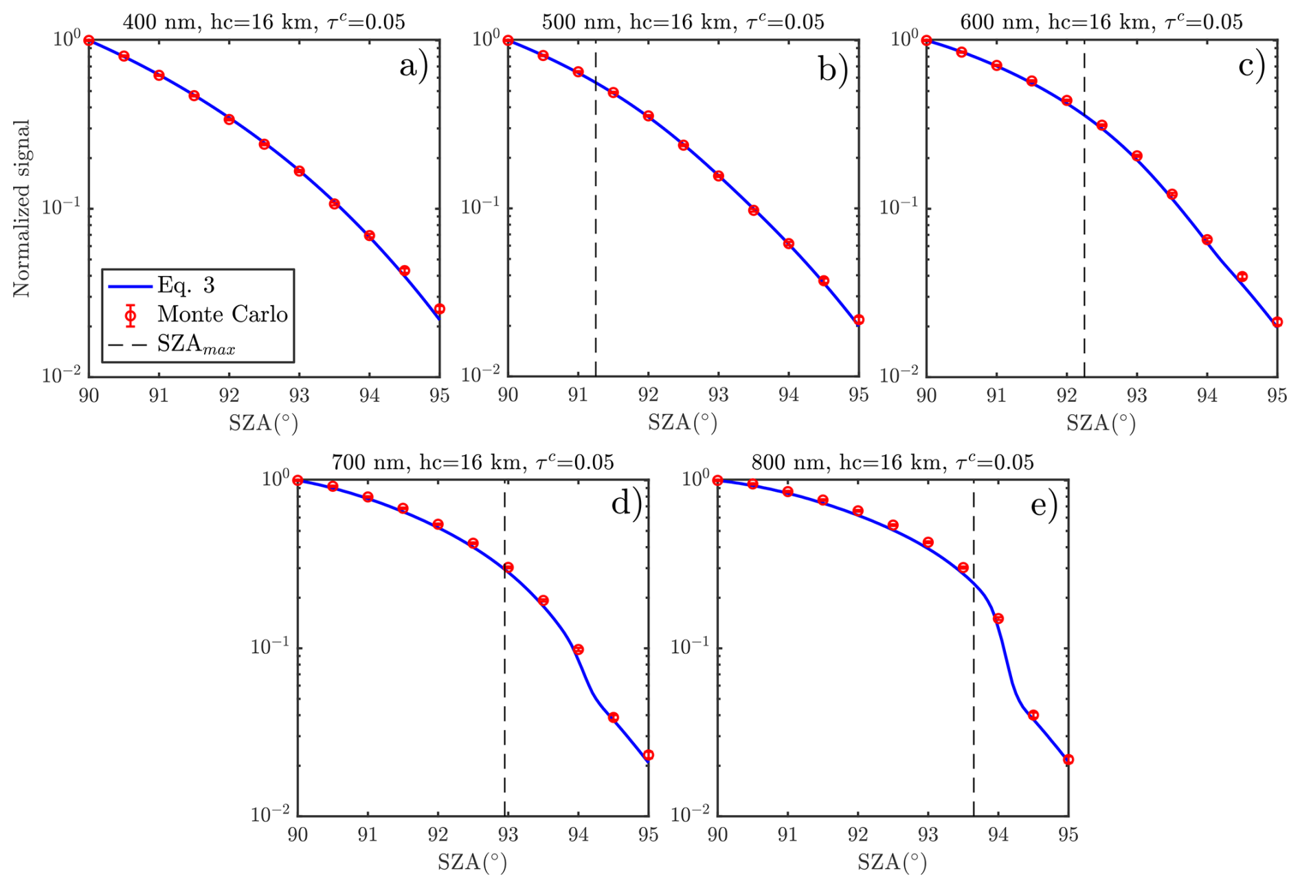
Figure 9 Similar simulations to those shown in Fig. 8, but keeping the cloud height fixed at h_C=16 km and varying the wavelength: 400 nm (a), 500 nm (b), 600 nm (c), 700 nm (d), and 800 nm (e). The remaining parameters are kept identical to those in Fig. 8. No dashed line is shown in (a), since ${\mathit{\lambda }}_{\mathrm{1}}={\mathit{\lambda }}_{\mathrm{2}}=\mathrm{400}$ nm and therefore SZA_max is not defined.

Figure 9 shows a comparison similar to that presented in Fig. 8, but in this case varying the wavelength from 400 to 800 nm in steps of 100 nm, while keeping the cloud height fixed at h_C=16 km. The remaining parameters are kept identical to those used in Fig. 8. In this scenario, the main wavelength-dependent contribution in the model arises from Rayleigh scattering, whose optical depth varies strongly with wavelength. As a result, the attenuation of the signal along the solar path changes accordingly, while the cloud contribution remains unchanged. This behaviour is clearly reflected in the curves, where the cloud-related feature becomes more pronounced as the wavelength increases. This is consistent with the decreasing contribution of Rayleigh scattering at longer wavelengths, which enhances the relative impact of the cloud on the observed signal. As in the comparison shown in Fig. 8, the SSM reproduces the Monte Carlo simulations with very good agreement across all wavelengths. In particular, the change in the structure of the cloud-induced feature in the intensity profiles is accurately captured by the SSM. Therefore, it is concluded that the main findings derived from the comparison in Fig. 8 can be consistently extended to different wavelengths.

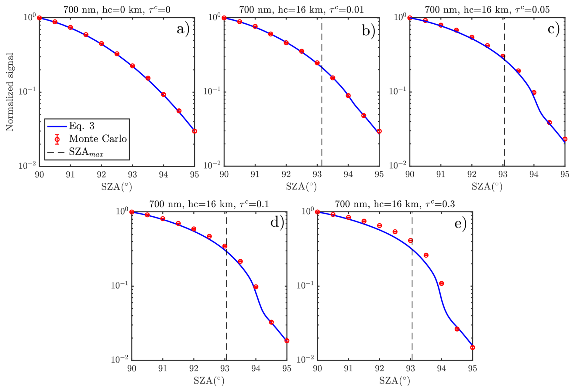
Figure 10 Same as in Fig. 8, but with the cloud height fixed at h_C=16 km and the cloud optical depth varied as follows: τ^C=0 (a), 0.01 (b), 0.05 (c), 0.1 (d), and 0.3 (e). All other parameters are identical to those used in Fig. 8. No dashed line is shown in (a), since no cloud is present and therefore no SZA_max can be defined.

Finally, a similar comparison was performed by varying the cloud optical depth from τ^C=0 (pure Rayleigh atmosphere) up to τ^C=0.3, as shown in Fig. 10. In all simulations, the cloud height is fixed at h_C=16 km and the wavelength at λ=700 nm, while the remaining parameters are kept identical to those used in Fig. 8. The lowest non-zero value considered for the cloud optical depth was τ^C=0.01. As discussed in the context of Fig. 9, the impact of the cloud is expected to be more pronounced at longer wavelengths, which would allow the detection of optically thinner clouds. However, since the objective of this section is to intercompare both models rather than to establish a detection limit, the wavelength and cloud optical depth range were fixed accordingly. The comparison shows that the agreement between both models progressively degrades as the cloud optical depth increases. While the SSM reproduces the Monte Carlo results very well for optically thin clouds (τ^C≲0.1), noticeable differences appear for larger optical depths. These discrepancies can be attributed to multiple-scattering effects within the cloud, which are not accounted for in the SSM.

In order to assess the impact of multiple-scattering effects on the retrieval of cloud height, Fig. 11 shows the relative rate of variation of P_Total(λ,SZA) with respect to SZA, computed for τ_C=0.3 and cloud altitudes of h_C=14, 16, and 18 km, together with the corresponding pure Rayleigh atmosphere. The retrieved value of SZA_max is determined by the intersection between the cloud and Rayleigh relative-variation curves. In these simulations, the Monte Carlo calculations were limited to SZA<94°. This choice is motivated by the high sensitivity of the relative variations of P_Total(λ,SZA) to the SZA sampling, which requires a fine angular resolution (ΔSZA=0.02°). As a consequence, the computational cost increases significantly as ΔSZA decreases, since a larger number of photons must be simulated to maintain a low level of statistical uncertainty. For this reason, the analysis is restricted to the SZA range of interest around the Rayleigh cutoff, where the determination of SZA_max is most relevant.

The results show that, despite the differences in the simulated normalized zenith intensities between the Monte Carlo model and the SSM observed in Fig. 10, the relative variations around the Rayleigh cutoff remain very similar in both cases. In particular, differences in SZA_max are found to be on the order of 0.12–0.15°, which correspond to uncertainties in the retrieved cloud height below 1 km, as will be discussed in the following sections. Thus, it follows that for cloud optical depths below τ_C∼0.3, the SSM is able to reproduce the Monte Carlo simulations with a satisfactory level of accuracy for the purpose of cloud-height retrieval. For optical depths approaching τ_C=0.3, the discrepancies increase, leading to uncertainties in cloud height of up to about 1 km. Based on this analysis, it is established that the SSM provides a reliable framework for the interpretation of twilight zenith intensity measurements and the retrieval of cloud heights for τ_C≲0.3. This range of optical depths is consistent with typical values reported for cirrus and PSCs (see, e.g., Kinne et al., 1989; Gil-Díaz et al., 2024), highlighting the potential of the SSM for application to real observations while avoiding the computational cost of full Monte Carlo simulations.

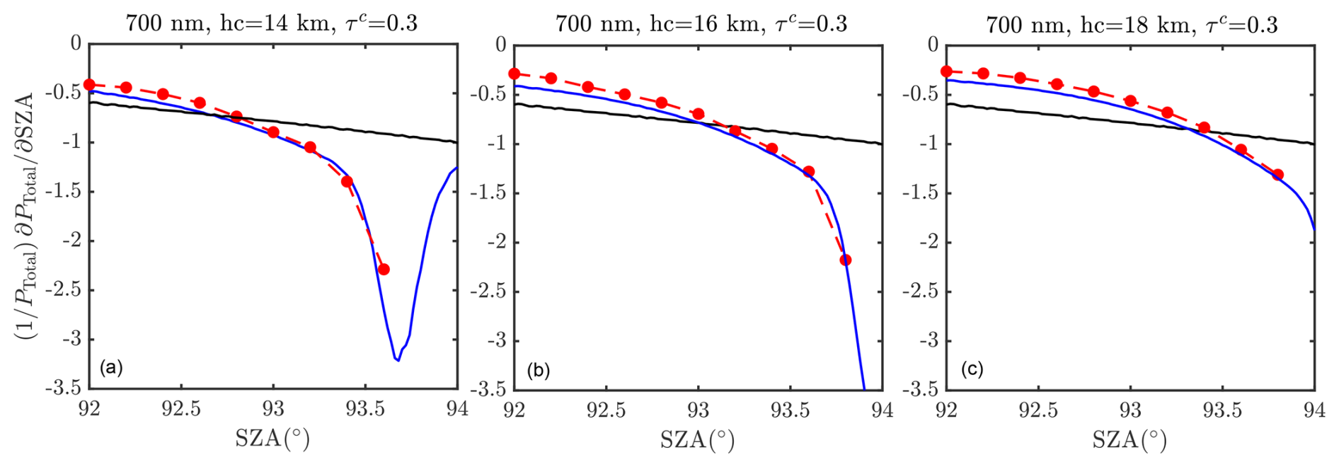
Figure 11 Comparison of the variation of $\left(\frac{\mathrm{1}}{P_{\mathrm{Total}}(\mathit{\lambda },\mathrm{SZA})}\frac{\partial P_{\mathrm{Total}}(\mathit{\lambda },\mathrm{SZA})}{\partial \mathrm{SZA}}\right)$ with SZA computed using the Monte Carlo model (red dots) and the SSM (blue solid lines) at 700 nm, for a pure Rayleigh atmosphere (black line) and different cloud scenarios with τ_C=0.3: h_C=14 km (a), 16 km (b), and 18 km (c). All other parameters are identical to those used in Fig. 8.

4 Sensitivity of cloud-height retrieval

Having validated the SSM against Monte Carlo simulations, it is now exploited its computational efficiency to investigate how uncertainties in atmospheric and cloud properties propagate into errors in the retrieved cloud height. Such an analysis would be computationally prohibitive using the Monte Carlo model due to its computational cost, but can be systematically explored within the present framework. The goal of this section is therefore to quantify the sensitivity of SZA_max, and consequently the inferred cloud height, to assumptions about cloud and atmospheric parameters. It is considered a reference atmospheric configuration consisting of a standard Rayleigh atmosphere and a single cloud layer located at 16 km, with an optical thickness of 0.05, a geometrical thickness of 2 km, and a horizontal scale of R_C=20 km. Starting from this baseline scenario, each parameter is varied individually in order to assess its impact on SZA_max. For each perturbation, the resulting shift in SZA_max is computed and subsequently translated into an error in the retrieved cloud height using the model. This approach allows us to directly quantify how uncertainties in atmospheric and cloud properties propagate into biases in cloud height retrieval. Since the CI maximum is determined by the relative SZA-variations of the zenith intensity (Eq. 16), all sensitivity tests are formulated in terms of this quantity rather than the absolute zenith intensity itself. In all simulations, the extinction due to the cloud is included following Eq. (19), thereby accounting for its horizontal distribution.

4.1 Sensitivity to cloud properties

First, the dependence of the cloud geometrical thickness on SZA_max is investigated. Figure 12a shows the relative rate of variation of P_Total with respect to SZA at 700 nm for different values of the cloud geometrical thickness, $\mathrm{\Delta }{h}_{\mathrm{C}}=\mathrm{1},\mathrm{2},\mathrm{3},$ and 4 km. In each case, SZA_max is defined by the intersection between the corresponding curve and the pure Rayleigh reference (black dashed line). The results show that increasing the cloud geometrical thickness significantly affects both the depth and the width of the minimum. However, these changes occur at SZA values larger than SZA_max. At SZAs close to SZA_max, all curves nearly overlap, indicating that the position of the CI^R maximum is largely insensitive to variations in Δh_C. This behaviour is confirmed quantitatively by the values of SZA_max. For a cloud height of 16 km, variations in Δh_C lead to changes smaller than 0.05°, which is comparable to the angular resolution used in these simulations. For lower cloud heights (12 and 14 km), slightly larger differences in SZA_max are observed when reducing the geometrical thickness from 2 to 1 km, reaching up to 0.15 and 0.1°, respectively. However, for Δh_C≥2 km, the variations in SZA_max remain below 0.05° in all cases. These angular differences translate into uncertainties in the cloud height smaller than 1 km.

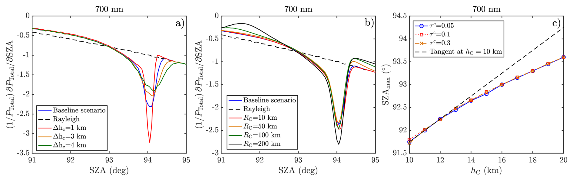
Figure 12 Sensitivity of SZA_max to cloud parameters: (a) variation with cloud geometrical thickness Δh_C, (b) variation with cloud horizontal scale R_C, and (c) relationship between cloud height and SZA_max for different cloud optical depths. The black dashed line in panel (c) represents the tangent to the τ_C=0.05 curve at h_C=10 km.

Next, the impact of the cloud horizontal scale, R_C, is investigated. Figure 12b shows an analysis analogous to that in Fig. 12a, but varying R_C from the baseline value of 20 km to 10, 50, 100, and 200 km. In all cases, the cloud height is fixed at 16 km and the optical thickness at τ_C=0.05. As expected, R_C has a noticeable impact on the relative SZA-variations of P_Total. As R_C increases, the extinction experienced by photons scattered along the line of sight becomes larger, reducing the contribution of P₁. This results in a deeper minimum and modifies the shape of the curves. However, in the SZA range between approximately 92.5 and 93°, all curves tend to converge. Importantly, this convergence occurs close to the intersection with the pure Rayleigh curve, which defines SZA_max. As a result, the variations in SZA_max remain limited despite the significant changes in the curve shape. By comparing the different cases, it is obtained a maximum variation of $\mathrm{\Delta }{\mathrm{SZA}}_{max}\approx \mathrm{0.1}$°, which translates into an uncertainty in cloud height of approximately 800 m. Similar analyses performed for other cloud heights show that the variations in SZA_max can reach up to 0.2° for h_C=12 km. This increase is consistent with the fact that, at lower altitudes, the CI maximum occurs at smaller SZA, where the solar beam propagates more horizontally and traverses a larger portion of the cloud before scattering. Despite these larger angular differences, the resulting uncertainty in cloud height remains of the same order (∼800 m).

To better understand this behavior, Fig. 12c shows the variation of SZA_max as a function of cloud height for τ_C=0.05, τ_C=0.1, and τ_C=0.3. The figure also includes the tangent to the τ_C=0.05 curve at h_C=10 km. It can be seen that the h_C–SZA_max relationship systematically lies below this tangent, indicating a sub-linear behavior. This implies that the sensitivity of SZA_max to cloud height decreases as altitude increases. This explains why, in the R_C sensitivity test, a variation of $\mathrm{\Delta }{\mathrm{SZA}}_{max}\approx \mathrm{0.2}$° at 12 km leads to a cloud-height variation comparable to that produced by a smaller $\mathrm{\Delta }{\mathrm{SZA}}_{max}\approx \mathrm{0.1}$° at 16 km. Figure 12c also shows that the h_C–SZA_max relationship remains essentially unchanged when the only parameter varied is the cloud optical thickness. This indicates that, in practical applications, τ_C can be kept fixed without introducing significant errors in the cloud-height retrieval. Consequently, any residual uncertainty associated with this parameter is expected to arise primarily from the use of the single-scattering model instead of the Monte Carlo approach. As shown in Sect. 3.5, these differences remain small and become only noticeable for optically thicker clouds (τ_C∼0.3), while still leading to cloud-height uncertainties below 1 km.

Finally, the impact of the cloud phase function on SZA_max is investigated. In particular, phase functions are computed using droxtals (quasi-spherical ice crystals with rounded edges) following the model of Yang et al. (2003, 2013), considering effective radii $r_{\mathrm{eff}}=\mathrm{5},\mathrm{10},$ and 20 µm. In this context, r_eff does not correspond to the effective radius of a volume-equivalent sphere, but rather to a geometrical parameter of a lognormal distribution defined in terms of the maximum crystal dimension (D_max), with $r=D_{max}/\mathrm{2}$. For the baseline scenario, the resulting values of SZA_max are 92.92, 92.96, and 93.00° for the three considered values of r_eff. According to the h_C–SZA_max relationship shown in Fig. 12c, these variations correspond to changes in cloud height of less than ∼ 300 m. These results indicate that the impact of the cloud phase function on the retrieval is non-negligible, but remains smaller than that of other parameters explored in this study. Therefore, uncertainties associated with the microphysical properties of the cloud particles are expected to have a secondary influence on the retrieved cloud height.

4.2 Sensitivity to aerosol properties

In all simulations presented so far, it has been considered a pure Rayleigh atmosphere together with the presence of a cloud layer. The next step is to investigate the impact of aerosols on SZA_max, and consequently on the retrieved cloud height. To this end, aerosols are introduced as a vertically distributed layer with an exponential decay characterized by a scale height H^A. The aerosol optical depth at the surface, ${\mathit{\tau }}_{\mathrm{0}}^{\mathrm{A}}$, together with H^A, are varied in order to assess their influence on the results.

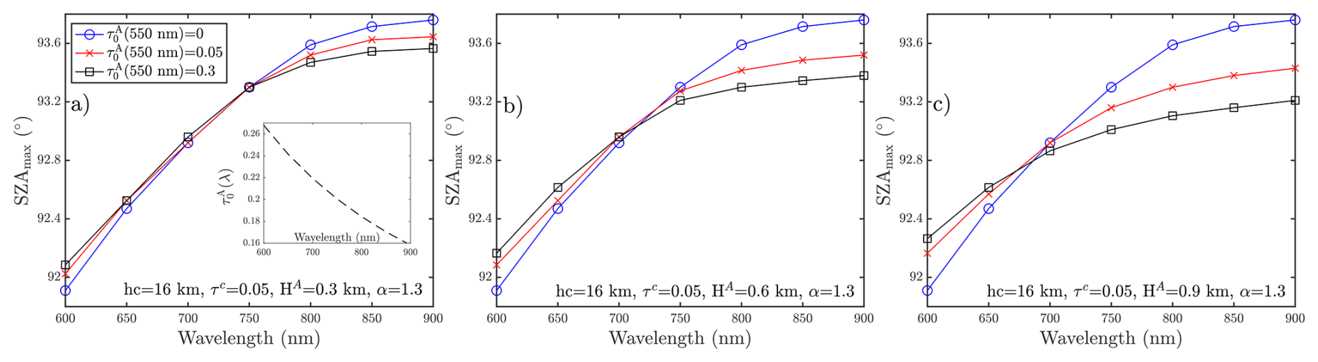
Figure 13 Variation of SZA_max with wavelength derived from CI^R for a cloud layer located at h_C=16 km with optical depth τ_C=0.05. Results are shown for different aerosol scenarios characterized by ${\mathit{\tau }}_{\mathrm{0}}^{\mathrm{A}}\left(\mathrm{550}\mathrm{nm}\right)=\mathrm{0}$ (blue line), 0.05 (red line), and 0.3 (black line), and for three aerosol scale heights: H^A=0.3 km (a), 0.6 km (b), and 0.9 km (c). The spectral dependence of ${\mathit{\tau }}_{\mathrm{0}}^{\mathrm{A}}$ is parameterized using an Ångström exponent α=1.3, whose corresponding curve is shown in the inset of (a).

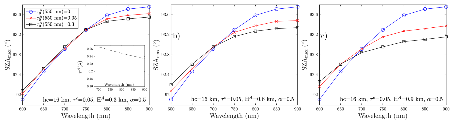
Figure 13 shows the variation of SZA_max with wavelength for a cloud layer with fixed altitude and optical depth of 16 km and 0.05, respectively. Different values of aerosol optical depth, ${\mathit{\tau }}_{\mathrm{0}}^{\mathrm{A}}\left(\mathrm{550}\mathrm{nm}\right)=\mathrm{0},\mathrm{0.05},\mathrm{0.3}$, and scale height, H^A=0.3, 0.6, and 0.9 km, are considered. In these simulations, the spectral dependence of the aerosol optical depth is described using an Ångström exponent of α=1.3. The results show that both the aerosol optical depth and the scale height have a clear impact on SZA_max, and therefore on the inferred cloud height. This effect becomes more pronounced at longer wavelengths (λ≳750 nm), where the Rayleigh optical depth is significantly reduced and the relative contribution of aerosols to the total attenuation becomes more important. However, as shown in Fig. 13, noticeable differences are also present at shorter wavelengths (e.g. 600 nm), indicating that aerosol effects are not negligible even in the visible range. To investigate the impact of the Ångström exponent on SZA_max, Fig. 14 shows simulations similar to those in Fig. 13, but for α=0.5. In this case, the aerosol optical depth decreases more slowly with wavelength over the spectral range considered, resulting in larger values at longer wavelengths. As in the previous case, larger values of ${\mathit{\tau }}_{\mathrm{0}}^{\mathrm{A}}$ and H^A lead to stronger variations in SZA_max, reaching up to ∼0.6° at λ=900 nm for H^A=0.9 km and ${\mathit{\tau }}_{\mathrm{0}}^{\mathrm{A}}\left(\mathrm{550}\mathrm{nm}\right)=\mathrm{0}$ and 0.3. By contrast, only minor differences are observed when varying the Ångström exponent between α=1.3 and α=0.5 (comparison between Figs. 13 and 14), indicating that ${\mathit{\tau }}_{\mathrm{0}}^{\mathrm{A}}$ and H^A are the dominant parameters controlling the variability of SZA_max in these simulations.

To quantify the impact on the retrieved cloud height, it is used a relationship similar to that shown in Fig. 12c. Under this assumption, a variation of $\mathrm{\Delta }{\mathrm{SZA}}_{max}=\mathrm{0.6}$° corresponds to an uncertainty of approximately 4 km in cloud altitude. This implies that, in a realistic aerosol scenario with ${\mathit{\tau }}_{\mathrm{0}}^{\mathrm{A}}\left(\mathrm{550}\mathrm{nm}\right)=\mathrm{0.3}$ and H^A=0.9 km, neglecting aerosols in the analysis (i.e., assuming ${\mathit{\tau }}_{\mathrm{0}}^{\mathrm{A}}\left(\mathrm{550}\mathrm{nm}\right)=\mathrm{0}$) would lead to an error of about 4 km in the retrieved cloud height. However, at 650–700 nm the variations in SZA_max are significantly smaller, with maximum values of $\sim \mathrm{0.08}-\mathrm{0.14}$° for H^A=0.9 km and ${\mathit{\tau }}_{\mathrm{0}}^{\mathrm{A}}\left(\mathrm{550}\mathrm{nm}\right)=\mathrm{0}$ and 0.3. These variations in SZA_max correspond to uncertainties of approximately 300–700 m in the retrieved cloud height. For smaller values of H^A, the differences in SZA_max tend to zero, and therefore the influence of aerosols on the cloud-height retrieval becomes negligible.

Figure 14 Same as in Fig. 13, but with an Ångström exponent α=0.5.

These examples demonstrate that, depending on the observational configuration (i.e., number of channels and selected wavelengths), the presence of aerosols and their vertical distribution can significantly affect the retrieval of cloud height. In this context, the selection of wavelengths around 650–700 nm is preferable, as indicated by the results presented above. However, due to the increase in Rayleigh optical depth at shorter wavelengths, the detection of lower-altitude clouds (below ∼16 km) becomes progressively more challenging as shorter wavelengths are considered. Multi-wavelength observations in the 650–900 nm spectral range provide an optimal compromise. Such observations would allow the spectral variation of SZA_max to be exploited in order to improve the accuracy of cloud-height retrievals, taking into account not only the presence of aerosols but also other cloud properties analyzed in the previous section.

These results highlight that analyses of this type are essential for defining an optimal cloud-height retrieval strategy tailored to a given observational configuration. In this context, the use of the SSM is particularly advantageous due to its negligible computational cost compared to Monte Carlo RT models. In practice, the computational efficiency of the SSM enables extensive sensitivity studies across a wide range of atmospheric scenarios, including variations in aerosol load, vertical distribution, and wavelength selection. Moreover, given its validity for optically thin clouds (τ^C≲0.3), the SSM allows full spectral simulations over the visible range to be performed at very low computational cost.

Finally, in the previous section, the differences between the SSM and the Monte Carlo model were shown to become significant mainly for cloud optical depths of τ^C≳0.3, due to multiple-scattering effects within the cloud that are not included in the SSM and that primarily affect the scattering term P₂. By contrast, the aerosol contribution enters mainly through P₁, for which the SSM reproduces the pure-Rayleigh behaviour accurately. Therefore, as long as the cloud optical depth remains within the range established in Sect. 3.5, the agreement between the SSM and the Monte Carlo model is not expected to change substantially in the presence of aerosols. This further supports the use of the SSM as a reliable and efficient tool for exploring the impact of aerosols and other atmospheric parameters on cloud-height retrievals.

5 Conclusions

In this paper, a methodology based on the single-scattering approximation is presented for the analysis of the color index (CI), defined in Eq. (1), derived from zenith intensity measurements during twilight for the study of high-altitude clouds. Based on the analysis carried out with this methodology, and its comparison with a Monte Carlo multiple-scattering model in spherical geometry, the following conclusions are drawn:

• The presence of high-altitude clouds during twilight produces a maximum in the CI (for λ₁<λ₂), whose position in terms of solar zenith angle (SZA) depends on the cloud altitude. The cloud introduces an additional scattering layer that enhances the zenith intensity at both wavelengths. However, due to the wavelength dependence of Rayleigh opacity, the attenuation of the signal is stronger at shorter wavelengths. As a result, the cloud becomes effectively dark at λ₁ at smaller SZAs than at λ₂, leading to an increase of the CI with SZA. This behaviour can be understood from the geometry of the solar path: for a given cloud altitude, the solar rays reaching the cloud traverse progressively lower atmospheric layers as SZA increases, resulting in a larger optical depth along the path. The CI reaches its maximum when the cloud contribution at λ₂ also starts to vanish. The exact value of SZA at CI maximum (SZA_max) corresponds to the condition where the relative variation of the zenith intensity with respect to SZA is equal at both wavelengths. This condition provides a direct physical interpretation of the origin of the CI maximum, linking it to the differential attenuation of radiation at the two wavelengths.

• The detection of clouds using the CI improves as the spectral separation between λ₁ and λ₂ increases. This is due to the strong wavelength dependence of Rayleigh opacity in the visible range: for wavelengths around λ₁∼400 nm, the Rayleigh optical depth is significant, which reduces the relative contribution of the cloud at λ₁ compared to λ₂. This leads to a stronger enhancement of the CI. In contrast, when both wavelengths are located in the red or near-infrared region (e.g., 700 and 800 nm), the cloud contribution is clearly visible at both wavelengths, resulting in a less pronounced CI maximum. Motivated by this behaviour, it is defined a new index, the Rayleigh-referenced color index, CI^R. Instead of using measurements at two wavelengths during the same twilight, this index relies on a single wavelength λ=λ₂, while the reference signal at λ₁ is replaced by the corresponding signal at λ₂ for a pure Rayleigh atmosphere. As in the case of the CI, the maximum of CI^R occurs at the SZA for which the relative variations of the zenith intensity with respect to SZA become equal, providing a consistent physical interpretation of the index. This index presents some advantages over the traditional CI:

  • (i)

    Only measurements at a single wavelength are required, allowing the use of narrow-band or single-wavelength instruments. For spectrometers, it also facilitates the selection of spectral regions free from strong gaseous absorption features;

  • (ii)

    The contrast of the cloud detection is enhanced in CI^R, since the Rayleigh reference does not include any cloud contribution. This advantage is particularly relevant when the instrument does not allow for a sufficient spectral separation between λ₁ and λ₂, in which case the performance of the traditional CI may be reduced.

  Consequently, the proposed Rayleigh-referenced CI provides a more flexible framework for future studies of optically thin high-altitude clouds, including cirrus and polar stratospheric clouds, using a broader range of observing systems.

• The single-scattering methodology (SSM) was compared with a reference Monte Carlo (MC) radiative transfer model previously used for twilight studies in the atmospheres of the Earth, Mars, and Titan. As expected, the single-scattering approximation becomes increasingly accurate as the cloud optical depth decreases, while maintaining a good agreement with the Monte Carlo model for cloud optical depths up to τ_C≈0.3. For τ^C=0.3, differences in SZA_max of about 0.1–0.2° are observed, which translate into errors in the retrieved cloud altitude smaller than 1 km. The main advantage of the SSM is its significantly lower computational cost compared to the Monte Carlo model, allowing the efficient exploration of a large number of simulations at different wavelengths and for different cloud geometries. Therefore, for cloud optical depths τ^C≤0.3, which is a representative range for high-altitude clouds such as cirrus or polar stratospheric clouds, the SSM provides a powerful and efficient tool for the rapid analysis of twilight zenith observations.

• Sensitivity tests were performed to assess the impact of the main cloud parameters on the retrieval of cloud altitude. In the model, the horizontal distribution of the cloud is assumed to follow a Gaussian profile, analogous to the vertical distribution, with the cloud extinction decreasing with distance from the observer zenith. In addition to the cloud optical depth and altitude, the model includes the parameters Δh_C and R_C, which define the vertical thickness and horizontal extent of the cloud, respectively. Variations of Δh_C between 1 and 4 km, and of R_C between 10 and 200 km, result in differences in the retrieved cloud altitude of approximately 800 m. In contrast, no significant variations in SZA_max are observed when the cloud optical depth is varied between τ^C=0.05 and 0.3. The impact of the cloud particle phase function was also evaluated by varying the effective radius between 5 and 20 µm. This results in changes in SZA_max equivalent to variations in the retrieved cloud altitude of about 300 m.

• Sensitivity analyses of aerosol properties show that aerosols can have a significant impact on the retrieval of cloud altitude, even for low optical depths. In particular, the aerosol optical depth ${\mathit{\tau }}_{\mathrm{0}}^{\mathrm{A}}$ and scale height H^A are identified as the dominant parameters controlling the variability of SZA_max, while the dependence on the Ångström exponent is comparatively weak. In the absence of independent information on aerosol properties, the selection of wavelengths less affected by aerosols, such as those around 650–700 nm, is recommended. Alternatively, the use of representative seasonal aerosol conditions may help reduce potential biases. In any case, the uncertainty in the retrieved cloud altitude associated with aerosol presence should be quantified, particularly in terms of ${\mathit{\tau }}_{\mathrm{0}}^{\mathrm{A}}$ and H^A, as these parameters can introduce errors of several kilometers under realistic atmospheric conditions.

The conclusions of this work are based on the comparison between the SSM and a Monte Carlo RT model previously validated for similar atmospheric conditions. Future work will focus on the application of this formulation to radiometric measurements, with the aim of directly validating the retrievals against independent cloud-height observations from lidar systems.