Employing smoothness of the time series of sky radiances measured in the solar aureole for cloud screening

Cloud screening algorithms have always been a critical component of Aerosol Robotic Network (AERONET) aerosol optical depth (AOD) Level 1.5 and 2.0 product. The initial cloud screening algorithm in the Version 1 and 2 database was semi-automatic and required involvement of a human analyst to finalize the results. It became fully automatic in Version 3 (V3) due to employing information on the angular shape of sky radiances measured in the aureole (curvature algorithm). Although efficient, the curvature algorithm is threshold based and fails to detect clouds when its parameters are beyond the corresponding pre-determined thresholds. This is especially noticeable at high latitudes where the size of ice crystals in cirrus clouds are sometimes relatively small and therefore comparable in size to aerosols. It is shown that additional information can be extracted from analysis of the smoothness of diurnal variability of sky radiances measured at the 3.3° scattering angle. This measurement is a part of the so-called curvature scan (CCS), which takes measurements from 3 to 7.5° scattering angle with 0.3° steps after each measurement of AOD. The analysis of the diurnal variability of CCS (3.3) for cloud-free conditions shows relatively smooth temporal dependencies, which can be fitted by polynomials with high correlation coefficients while in conditions almost completely dominated by clouds, the temporal variability is completely random. For partially cloudy days, the two main features are observed: relatively smooth aerosol signatures and irregular spikes due to clouds. The new technique is proposed that employs the smoothness of the diurnal variability of the CCS(3.3) scan as a criterion of the cloud free conditions. In the case when both features are present, the idea of the new algorithm is to remove irregular spikes due to clouds while keeping the smooth part due to aerosols intact. The new algorithm detects spikes associated with clouds by comparing magnitudes of CCS(3.3) at neighboring time stamps through calculating their first differences (FD). This algorithm was applied to the CCS(3.3) measurements taken at several AERONET sites. The results were analyzed in terms of net change in Angstrom exponent (AE) as well as number of AOD measurements. The analysis showed the algorithm performs satisfactorily at AERONET sites dominated by fine mode aerosols, however at sites dominated by dust, the algorithm removes a big fraction of cloud-free observations. The issue was corrected by introducing an additional cloud screening parameter. It is based on observation of the different rates in changing of AE with iterations for cloud-free and cloudy conditions with a much higher rate in the former case. The new parameter was selected as a slope of the linear regression between integration number and the value of AE after the corresponding iteration. The algorithm disregards FD algorithm results if the slope is smaller than certain threshold value. Finalizing the FD algorithm threshold setting as well as evaluation of the algorithm performance is done by using independent cloud detection information available from Micro-Pulse Lidar Network (MPLNET) data. The AERONET and MPLNET data were time and space collocated with additional averaging over a one-hour period. The comparison showed that, on average, the FD algorithm outperformed V3 L1.5 by about 0.02 in Matthews Correlation Coefficient (MCC), suggesting consistent improvement in overall cloud detection accuracy. Additional analysis performed in terms of MCC metrics also showed that the FD algorithm achieves a more balanced and accurate classification of clouds vs clear.

1 Introduction

The Aerosol Robotic Network (AERONET) has been routinely providing accurate measurements of spectral aerosol optical depth (AOD) since the network started in 1993 (e.g. Holben et al., 1998; Eck et al., 1999). The AOD product is valuable in numerous applications, for example, analysis of aerosol effects on Earth climate through aerosol radiative forcing as well as validation of satellite AOD retrievals. Also, spectral AOD measurements along with those of the sky radiances constitute an input to the AERONET aerosol retrieval code (Sinyuk et al., 2020). A major requirement of high quality AOD measurements is that they should be provided in cloud – free conditions therefore relatively free of cloud contamination effects. It is important because of misperception of optically thin clouds as aerosols can seriously obscure aerosol optical properties. Therefore, cloud screening procedures have always been a critical component of the AOD product in AERONET.

The first AERONET cloud screening algorithm was primarily based on temporal variability of AOD measurements as well as on a number of additional checks which are described in detail in Smirnov et al. (2000). The main shortcoming of this algorithm was in it being semi-automatic and therefore requiring involvement of a human analyst to finalize the AOD cloud clearing. The algorithm became fully automatic in Version 3 (V3) of cloud screening by additionally utilizing sky radiances measured in the solar aureole for thin cirrus detection. The new algorithm employs information on the angular shape of solar aureole measurements which was parameterized by the curvature of the angular dependence of measured aureole sky radiances (e. g. Giles et al., 2019). The algorithm utilizes two thresholds which were determined by comparison of the results of the new algorithm to time and space collocated lidar data (Giles et al., 2019). In conjunction a new scan scenario called curvature scan (CCS) was designed and implemented in new instruments for more efficient application of the new cloud screening algorithm. This CCS scan takes measurements from 3 to 7.5° scattering angle with 0.3° steps after each measurement of AOD (Giles et al., 2019). The shortcoming of the new algorithm was found in some instances when thin cirrus clouds calculated curvature values were beyond operational thresholds. In particular, the V3 algorithm frequently fails to detect clouds at high latitude AERONET sites where the sizes of ice crystals may be smaller at times and therefore comparable in magnitude to that of aerosols. In this paper, we suggest an improvement in the V3 algorithm by further exploring the potential of employing sky radiance measurements in the aureole. Specifically, we propose employing the smoothness of diurnal variability of sky radiances measured by the CCS scan only at the 3.3° scattering angle. The new algorithm is based on assumption of smooth temporal variability of 3.3° CCS measured sky radiance at 1020 nm in the absence of clouds. The physical rationale for this assumption is that temporal variability is equivalent to variability due to variation in solar zenith angle (SZA) which is relatively smooth based on radiative transfer simulations for an aerosol laden atmosphere. The new algorithm inputs time series of CCS(3.3) sky radiances for the entire day, detects spikes due to clouds and marks AOD associated with spikes as cloud contaminated.

The paper is organized as follows: section two reviews the existing V3 curvature algorithm and presents analysis of its shortcomings. Section three describes the concept of employing smoothness of the time series of CCS measurements for cloud detection, section four presents detailed description of the algorithm, while section five discusses algorithm application to select AERONET sites and cases and introduces an additional algorithm parameter which helps to reduce erroneous removal of aerosols. Section six presents algorithm validation by comparing the results to time and space collocated lidar data and also discusses final tuning of the algorithm thresholds. Section seven presents a summary and conclusions of this study.

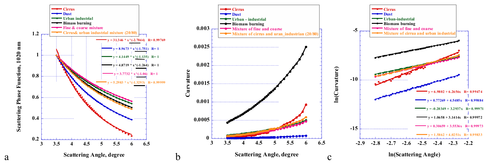
Figure 1 Scattering phase function calculated for different atmospheric particulates. Solid lines represent power law fit (a), Dependence of the curvature on the scattering angle in aureole calculated for three typical fine and coarse mode dominated aerosols, fine-coarse aerosols and aerosol-cirrus mixtures (b), Slope of the curvature in aureole estimated for three typical fine and coarse mode dominated aerosols, fine-coarse aerosols and aerosol-cirrus clouds mixtures (c).

2 Review of the curvature algorithm

The solar aureole curvature algorithm is an essential part of the cloud screening algorithm of AERONET Version 3 allowing for fully automatic cloud screening procedure of the direct Sun measurements of AOD. It is particularly important in the case of spatially and temporally homogeneous cirrus clouds that often pass the other cloud screening checks that rely on temporal variance. The technical aspects of the algorithm are described in detail in Giles et al. (2019). Here we review the physical ideas underlying the curvature algorithm which could be helpful in understanding its shortcomings as well as improvements suggested in this paper.

The concept of employing sky radiances measured in the solar aureole for cloud detection is based on the dependence of their angular shape on sizes of atmospheric particles (aerosols and/or ice crystals). The idea is illustrated in Fig. 1a,which depicts the angular shape of scattering phase functions for aerosols, cirrus clouds, and mixture thereof. It shows scattering phase functions in the range of the scattering angles from 3.5 to 6° calculated for selected aerosol types: desert dust, biomass burning, urban-industrial, the mixture of fine and coarse mode aerosols. These scattering phase functions were calculated using size distributions and complex refractive indexes retrieved by the AERONET operational inversion code at locations dominated by the corresponding aerosol types: Tamanrasset (Algeria, dust aerosols), Mongu (Zambia, biomass burning), GSFC (USA, urban-industrial, Kanpur (India, fine-coarse mixture). Figure 1a also displays scattering phase function for cirrus cloud crystals and mixture of cirrus/urban-industrial aerosols in proportion 20 to 80. Ice crystals scattering phase function was taken from the “Spectrally consistent scattering, absorption and polarization properties of atmospheric ice crystals at wavelengths from 0.2 to 100 µm” database by Ping Yang et al. (2026). All the scattering phase functions are calculated for 1.02 µm and normalized to the 3.5° scattering angle value. The 1.02 µm wavelength of AERONET was selected due to the smallest contribution of molecular scattering among the four standard wavelengths used for sky radiance measurements: 0.44, 0.675, 0.870, and 1.02 µm.

All of these phase functions are fitted by the power law (solid lines) with equations and correlation coefficients displayed in Fig. 1a. It shows that shapes of the scattering phase functions are different for different particulates as characterized by the slope of a power fit. In particular, the ice crystals and desert dust aerosols are clearly separated from other aerosol types as well as “partially cirrus contaminated ” urban industrial aerosols. These results support the idea that shape of sky radiances in the solar aureole can be used to distinguish aerosol from ice crystal clouds under appropriate shape parametrization.

Figure 1a shows the power fit of scattering phase functions assuming the single scattering approximation in aureole provides a rather accurate approximation to its angular shape with correlation coefficients close to one. This is a well-known fact which is called the van de Hulst approximation, (see for example Sviridenkov, 1993 and references therein). The power fit approximation might still be accurate in the presence of a multiple scattering; however, we are not aware of its validation in realistic atmospheric conditions under typical ranges of variability in observation geometry and aerosol optical depth. Therefore, we adopted a general parametrization of angular shape of the scattering phase function in aureole based on the curvature which is a parameter used in differential geometry to characterize a shape of a two-dimensional curve (e. g. Casey, 1996). The curvature describes for any part of a curve how much the curve direction changes over a small distance travelled (e.g. angle in radians/meter), so it is a measure of the https://en.wikipedia.org/wiki/Instantaneous_rate_of_change (last access: 18 September 2026) of direction of a point that moves on the curve: the larger the curvature, the larger this rate of change. In other words, the curvature measures how fast the unit tangent vector to the curve rotates (fast in terms of curve position) (Wikipedia). It can be better understood using the radius of curvature which is the reciprocal of the curvature and equals the radius of the circular arc which best approximates the curve at this point (Wikipedia). In this interpretation, for a straight line the radius of the curvature is an infinity, and the curvature is equal to zero. For a two-dimensional curve described by a function y=f(x), the curvature is defined by the following equation:

$$\begin{array}{}\text{(1)}& k={\displaystyle \frac{\ddot{y}}{(\mathrm{1}+{\dot{y}}^{\mathrm{2}}{)}^{\mathrm{3}/\mathrm{2}}}},\end{array}$$

where $\ddot{y}$ is the second derivative of y, $\dot{y}$ is the first derivative of y, and k stands for the curvature. In the AERONET Version3 cloud screening algorithm the curvature was selected to parameterize the angular shape of sky radiances in the aureole.

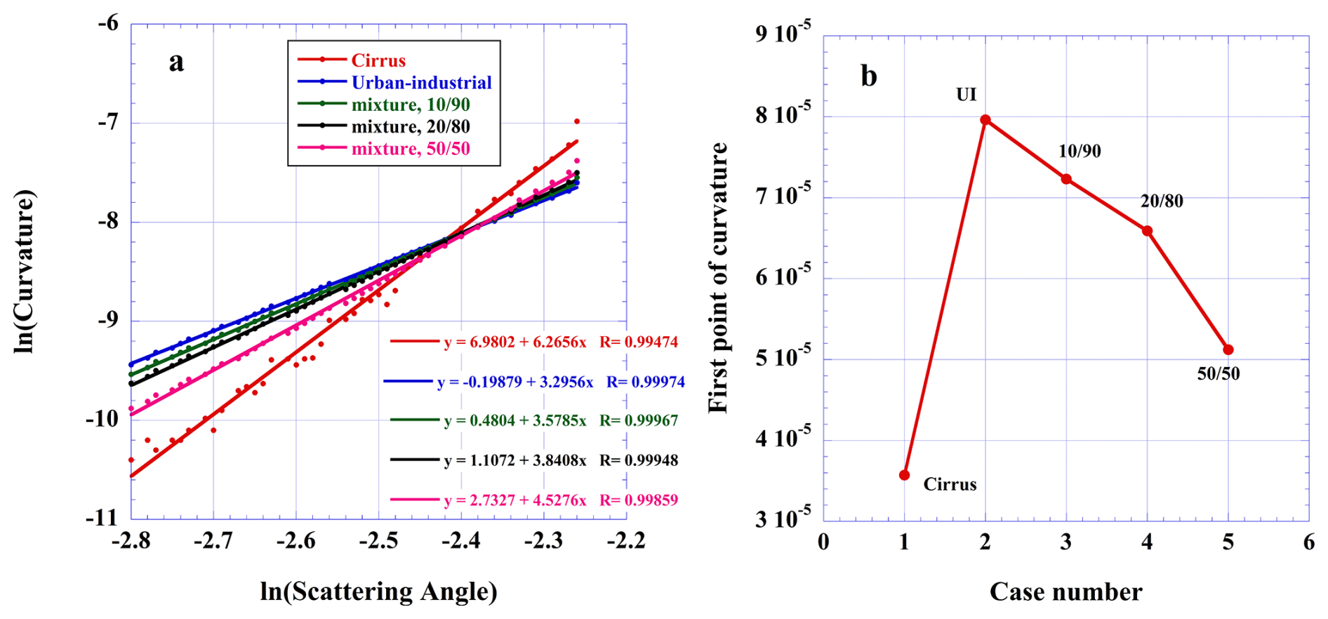
Figure 2 Dependence of the curvature slope on the cloud fraction for the three mixtures of urban industrial aerosol with cirrus clouds, (cirrus clouds/aerosols): 10/90, 20/80, and 50/50 (a), dependence of the first point of the curvature on case number, each case corresponding to the different cloud fraction for the mixture of urban-industrial aerosols with cirrus clouds (b).

Figure 1b shows dependencies of the curvature on the scattering angle in the aureole calculated for the scattering phase functions shown in Fig. 1a. The general trend for all the cases considered is an increase of the curvature with the scattering angle. The magnitude of the curvature, however, is quite different for different types of particles with strongly absorbing biomass burning and desert dust aerosols displaying the largest and the smallest magnitudes respectively. For other types of aerosols, the magnitudes of the curvature are close to each other. However, it is noticeable that the rate of the increase (slope) of the curvature at larger scattering angles is rather different for the ice crystals and aerosols, which can be used as an indicator of the presence of clouds. Figure 1c shows the dependencies displayed in Fig. 1b but on the ln-ln scale, where natural logarithms were taken from scattering angles in radians. Each particle type dependence is accurately approximated by a linear fit with high correlation coefficients. This representation provides clear separation between aerosol particles of different sizes in terms of a slope of the curvature. For example, slope of the curvature for desert dust aerosols (4.55) could be selected as a threshold for aerosols above which the sky radiances are considered as originated from scattering by cirrus clouds. However, for some cloud aerosols mixtures, magnitudes of the curvature slope could be below this threshold and will not be detected: 4.03 for cirrus/urban-industrial mixture is below 4.55 for dust. Therefore, extra information is needed to detect partial cloud contamination for cloud/aerosol mixtures.

Figure 2a shows dependencies of the slope of the curvature in ln-ln scale for cirrus clouds, urban industrial aerosols and three cloud/aerosol mixtures in proportions 10/90, 20/80, 50/50. It can be seen that the magnitude of the slope of the curvature is increasing with increasing cloud fraction but still stands below the curvature slope threshold of 4.55 for dust. Another change is the decreasing of the slope of the curvature magnitude at the smallest scattering angle which is the consequence of the forward peak being shifted into the narrower range of the scattering angles as cloud fraction increases. Figure 2b shows the change in the magnitude of the curvature at the smallest scattering angle as a function of a case number with each case corresponding to the different cirrus cloud fraction. Similar behavior was observed in numerical simulations for biomass burning aerosol (not shown). Both analyses demonstrate sensitivity of the curvature magnitude at the first scattering angle to the cloud fraction contaminating AOD measurements.

The slope of the curvature along with the curvature magnitude at the smallest scattering angle, named simply the first point, were selected as parameters for the part of AERONET Version 3 cloud screening algorithm employing aureole measurements of sky radiances at 1.02 µm. In preliminary testing of the curvature algorithm, the aureole part of the almucantar (ALM) and principle plain (PP) scans between 3.2 and 6° were used. They normally include from four to five scattering angles depending on the solar zenith angle (SZA) and the derivatives in Eq. (1) were calculated numerically. For the latest T version of Cimel sun photometers the new measurements protocol named curvature scan (CCS) was implemented. It takes measurements from 3 to 7.5° scattering angle with 0.3° steps after each measurement of AOD (Giles et al., 2019). Due to these small angular increments, the CCS scans exhibited small angular oscillations which result in substantial noise in curvature calculated numerically. Therefore, it was decided to fit CCS measurements by a power law which is a good approximation for scattering phase functions in the aureole region for scattering angles smaller than 6° (Sviridenkov, 1993). However, to ensure the accuracy of the fit in the presence of multiple scattering and to filter out CCS measurements with high noise, the correlation coefficient of the power fit was required to be larger than 0.98. In this case derivatives can be taken analytically and the expression for the ln of the curvature takes the following form:

$$\begin{array}{}\text{(2)}& \ln k=a+\left(\mathrm{1}-\mathrm{2}b\right)\ln \mathit{\phi },\end{array}$$

where k stands for curvature, φ denotes scattering angle in radians and a and b are parameters of power fit y=aφ^b. So, the curvature slope is defined as 1−2b, and the first point is calculated using Eq. (2) for the scattering angle 3.3°. The 3.0° scattering angle is not used to avoid stray light contamination. In AERONET Version 3, the thresholds for both slope of the curvature and the first point were selected using the Micro-Pulse Lidar Network (MPLNET) (e. g. Welton et al., 2001) lidar cloud identification database which is discussed in detail in Giles et al. (2019). The lower threshold for the slope of curvature was selected at 4.2 and the upper threshold for the first point at $\mathrm{2}\times {\mathrm{10}}^{-\mathrm{5}}$.

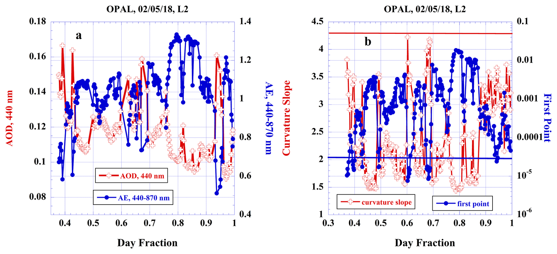
Figure 3 Temporal dependence of level 2 AOD measured at OPAL AERONET site on 2 May 2018 (a), slope of the curvature and the first point of curvature calculated from CCS (3.3) measurements (b).

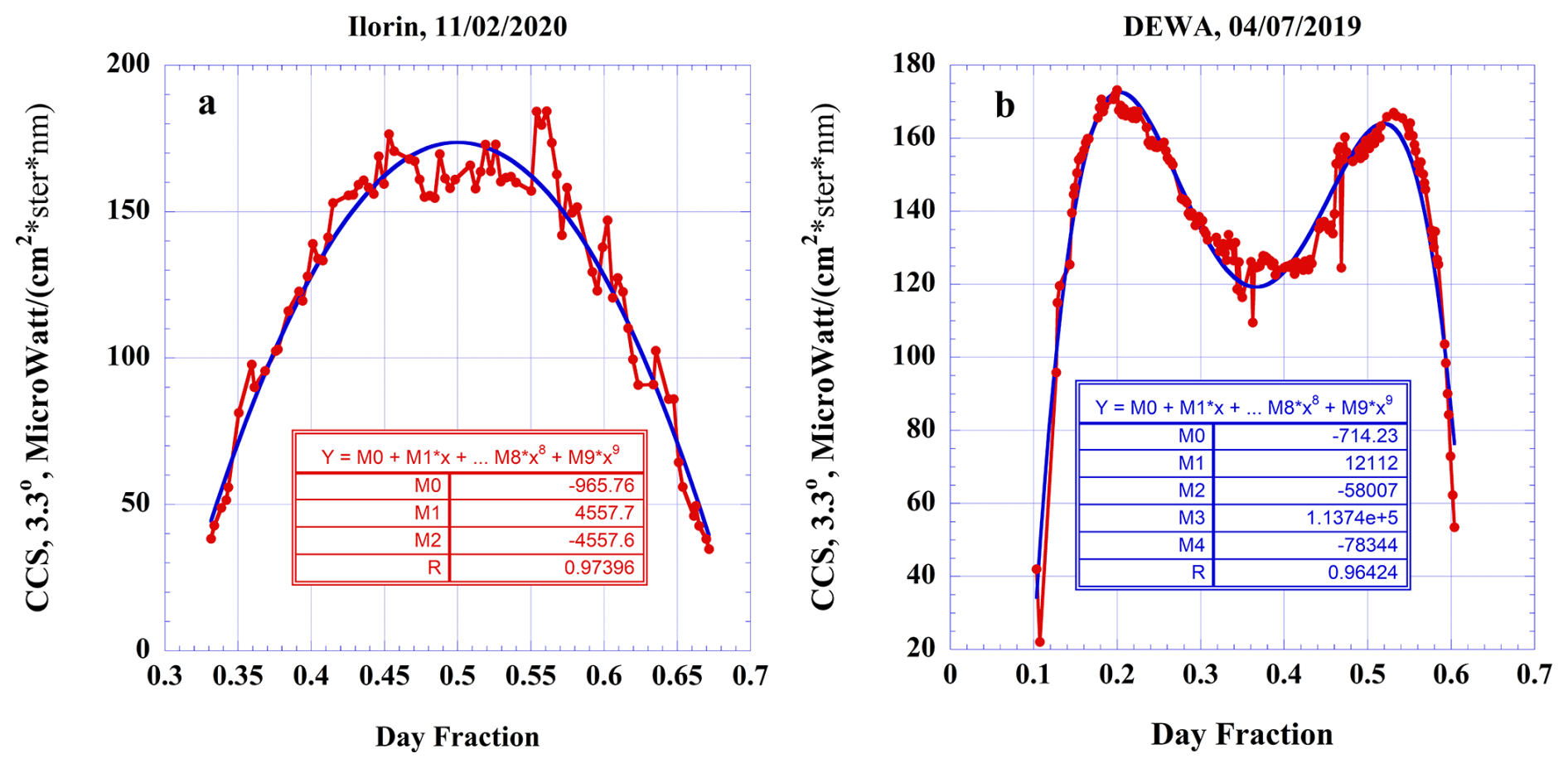
Figure 4 Temporal dependence of CCS (3.3) measured at (a) Ilorin AERONET site on 11 February 2020, (b) DEWA AERONET site on 4 July 2019.

Figure 5 Temporal dependence of CCS (3.3) measured at DEWA AERONET site on 18 July 2019.

Due to this being a threshold-based method, the curvature algorithm fails cloud detection in cases with curvature slope values below or the first point values above the corresponding threshold values. For example, Fig. 4c from Giles et al. (2019) shows that about one third of AERONET/MPLNET coincident cloud contaminated data to the left of the dashed line will not be detected after applying both thresholds. Figure 3a shows an example of the curvature algorithm failing cloud detection at the OPAL AERONET site (Eureka, Canada, 80.05° N) on the second of May 2018. Figure 3a shows the time series of AOD after the V3 cloud screening algorithm was applied (Level 2), and variability of Angstrom exponent (AE; 440–870 nm) throughout the day. The main feature of Fig. 3a is the strong correlation between upward spikes in AOD and downward spikes in AE for the same times of observations. The sharp decrease in AE can be explained by the effect of undetected clouds due to the size of cloud crystals being much larger than that of aerosols. Simultaneously, the clouds presence results in substantial spikes in AOD. Figure 3b shows time series of the slope of the curvature and the first point corresponding to the time series of Fig. 3a. As can be seen, both parameters exhibit sharp spikes: upward for the slope of the curvature and downward for the first point which are indicative of the cloud presence. However, most of the spikes are below (slope of the curvature) or above (the first point) the corresponding thresholds and so clouds giving rise to these spikes were not detected by the curvature algorithm. A similar picture was observed at a number of high latitudes AERONET sites in north Canada, Greenland and the Arctic. The fact that clouds were not detected at these locations by the AERONET V3 algorithm is most probably in part due to cirrus clouds being composed of small ice crystals with sizes comparable to those of aerosols. The possibility of cirrus clouds being composed of relatively small ice crystals at colder northern latitudes was confirmed by in situ measurements by Kramer et al. (2009). Figure 5 of that paper shows that the size of ice crystals is decreasing as ambient temperature decreases reaching the values of integral ice crystals radius as low as ∼ 3 µm in the Arctic. Furthermore, Kramer et al. (2020) showed in situ aircraft measured cirrus cloud mean mass radius varying from 1 to 200 µm. To overcome these shortcomings of the curvature algorithm, additional information is needed to screen cirrus clouds.

3 Smoothness of time series of CCS measurements

The analysis of the OPAL AERONET site case demonstrates that although the majority of clouds were not detected by the way of comparison of the curvature parameters to thresholds, the cloud presence manifests itself in sharp spikes of both AOD and AE in their time series. This implies that in cloud-free conditions the corresponding time series should be smoother. Thus, non-smooth temporal variability of the curvature parameters as well as AE could be considered as an indication of cloud contamination of AOD measurements and used for cloud detection. The curvature parameters as well as AE are derived from the measurements of sky radiances and AOD respectively. The curvature is very sensitive to the measurement noise while the accuracy of AE depends on the magnitude of AOD relative to the AOD uncertainty. Therefore, it would be preferable to use measurements themselves. In particular, temporal non-smoothness of CCS measurements of sky radiances at 3.3° scattering angle could be used as a criterion for cloud detection. The physical rationale for smooth time variations of CCS (3.3) measurements is that CCS temporal changes are due to the change in the solar zenith angle (SZA) in which case radiative transfer calculations will predict smooth temporal behavior of modelled radiances.

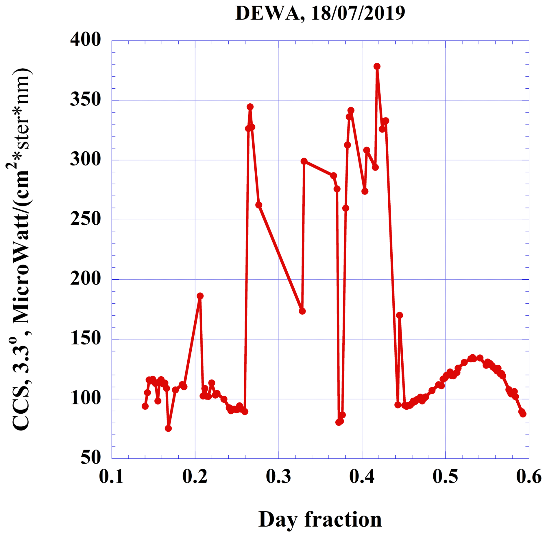
Figure 4 shows examples of temporal variability of CCS (3.3) measured at two different AERONET sites under cloud free conditions; (a) Ilorin, (Nigeria, 11 February 2020), (b) DEWA Research Center (United Arab Emirates, 4 July 2019). The aerosol loading at Ilorin site is dominated by dust with very high AOD: 2.5 ± 0.18 at 0.44 µm (AE ∼ 0.21 ± 0.018). The temporal dependence of CCS (3.3) is accurately fitted by a second order polynomial with high correlation coefficient. The random variability around the polynomial fit is due to temporal variability of aerosols. The CCS (3.3) dependence measured at DEWA site is also dominated by dust with AOD at 0.44 µm of 0.914 ± 0.1 (AE ∼ 0.42 ± 0.07) and is rather accurately approximated by polynomial of fourth order with high correlation coefficient. The common feature in both cases is the presence of a rather smooth temporal aerosol signature interposed by random noise due to natural variability of aerosols. Figure 5 shows the CCS (3.3) temporal dependence measured at DEWA site on 18 July 2019, when clouds were present part of the day. Two main features of Fig. 5 are the smooth part due to aerosols with little or no clouds and the irregular spikes due to clouds. In cases like that when both features are present a cloud screening algorithm could be based on removing spikes due to clouds while keeping the smooth parts intact. The cloud screening procedure introduced in this paper is based on this idea.

4 Algorithm description

The proposed algorithm inputs a time series of CCS (3.3) for the entire day with minimum three measurements required to detect spikes associated with clouds and distinguish these spikes from those due to natural variability of aerosols. Simply put the algorithm compares the magnitude of CCS (3.3) at neighboring time stamps. Technically it is done by calculating the first differences of measured sky radiances:

$$\begin{array}{}\text{(3)}& \mathrm{FD}\left(i\right)=I\left(i+\mathrm{1}\right)-I\left(i\right),i=\mathrm{1},\mathrm{\dots },M-\mathrm{1},\end{array}$$

where M is the number of measurements for the day and I(i) is a CCS (3.3) measured at a time stamp i. It should be noted that no preliminary detrending using a polynomial fit was used. If FD values are above some threshold, the measurements contributing to the spikes will be marked as cloud contaminated. A threshold for FD cloud screening can be estimated from CCS (3.3) data measured in a cloudless day. Due to being based on using first differences of aureole sky radiances at 3.3°, the algorithm was abbreviated as FD.

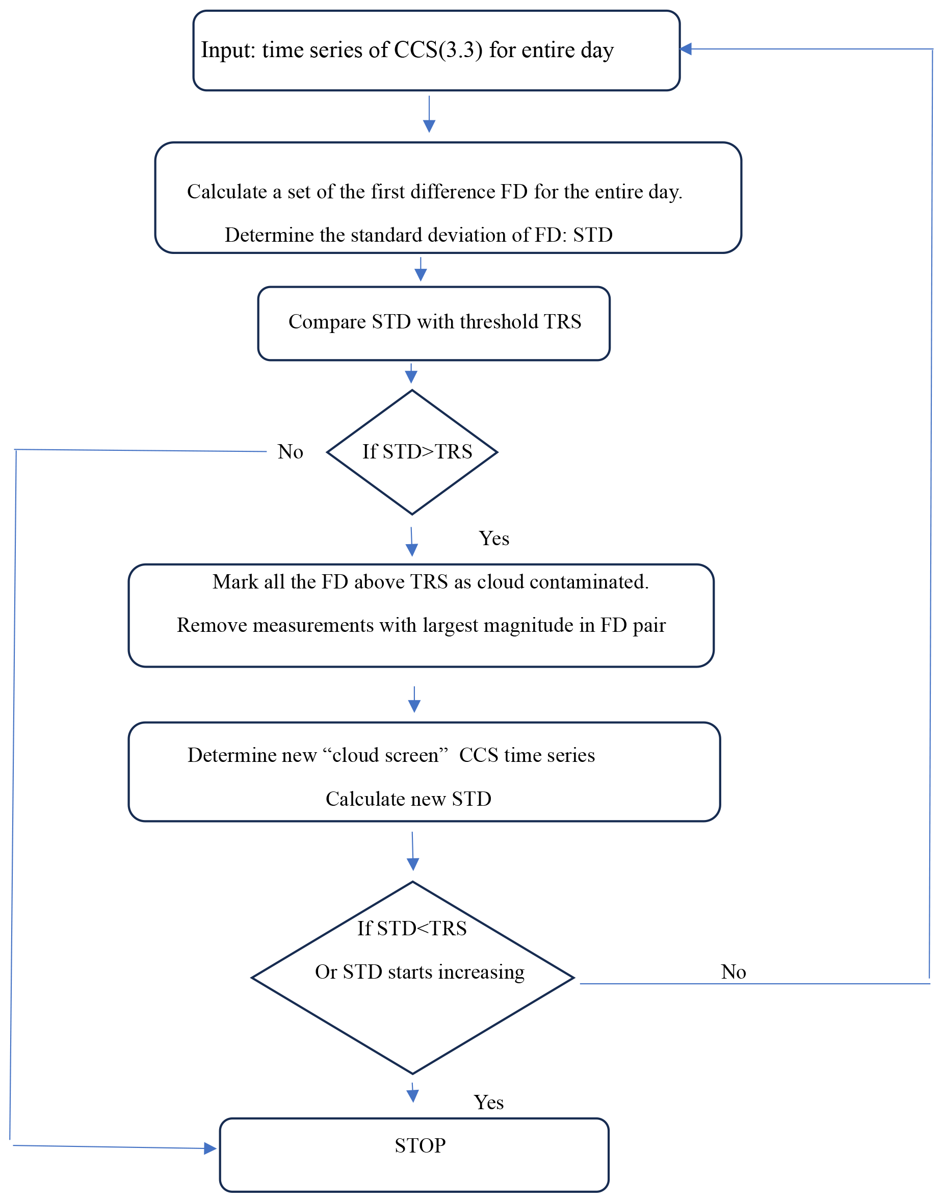
Figure 6 shows a flow chart of the FD algorithm. For the first step, the first differences of CCS (3.3) measurements are calculated for an entire day. It was found that instead of using a threshold in terms of FD values it is more efficient to use the standard deviation of the first differences. Therefore, the standard deviation (STD) is calculated and compared with a threshold standard deviation value estimated for cloudless days (TRS). If STD is greater than TRS, the algorithm marks all the first differences that are above TRS as cloud contaminated. For those FDs which are larger than TRS, the algorithm removes measurements of AOD corresponding to CCS (3.3) with the largest magnitude in FD each pair thereby producing the first iteration “cloud screened” time series for which a new value standard deviation is calculated. Iterations continue while the standard deviation after each iteration is decreasing and also above TRS. As soon as STD is below TRS, or it starts increasing then the algorithm stops. Increasing of STD means that the algorithm is no longer removing irregular spikes associated with clouds and CCS (3.3) variability is mostly random which could be either due to variability of aerosols or alternatively cases completely dominated by clouds with no apparent temporal cloud free aerosol signature. If during iterations, FD connects measurements separated by temporal gaps, and the FD value is larger than TRS, the algorithm will then remove the AOD value corresponding to the CCS measurement with the largest magnitude. These situations are conceptually similar to the cases of temporally adjusted measurements and should not create any additional problems.

Figure 6 Flow chart of FD algorithm.

It should be noted that there is diurnal variability in FD even in cloud free conditions which is predominately due to the variability in the SZA as can be seen from Fig. 4 for polynomial fits of CCS measurements versus time. However, TRS for cloud free 3.3° sky radiances already includes, at least partially, this SZA variability. Figure 7 shows distributions of FD calculated from CCS measurements at the DEWA AERONET site: (1) 4 July 2019 (cloud free conditions, Fig. 4b) (red line), (2) polynomial fit to these measurements (blue line), and (3) 18 July 2019 (partial cloudy day, Fig. 5) (green line). As can be seen from the plot STDs in cases (1) and (2) are finite due to SZA variability. The spikes at 3.3° measured radiances in case (3) resulted in the shoulders in the corresponding FD distribution which exceeded the STD for both cases (1) and (2) and consequently will be removed by the algorithm. The STDs corresponding to the different FD distributions are shown on the plot in corresponding colors. The threshold for TRS was selected from comparison of FD algorithm results to MPLNET cloud detection and found to be 3.0, as described in Sect. 6. This value, on average, accounts for the natural FD variability in cloud free conditions. Figure 7 also shows that the mean value of the FD diurnal variability is close to zero due to the symmetry in FD diurnal dependence on SZA. It is true even in Fig. 7 case (3) where large irregular spikes in 3.3° radiances are present (the mean value is ∼ 0.06).

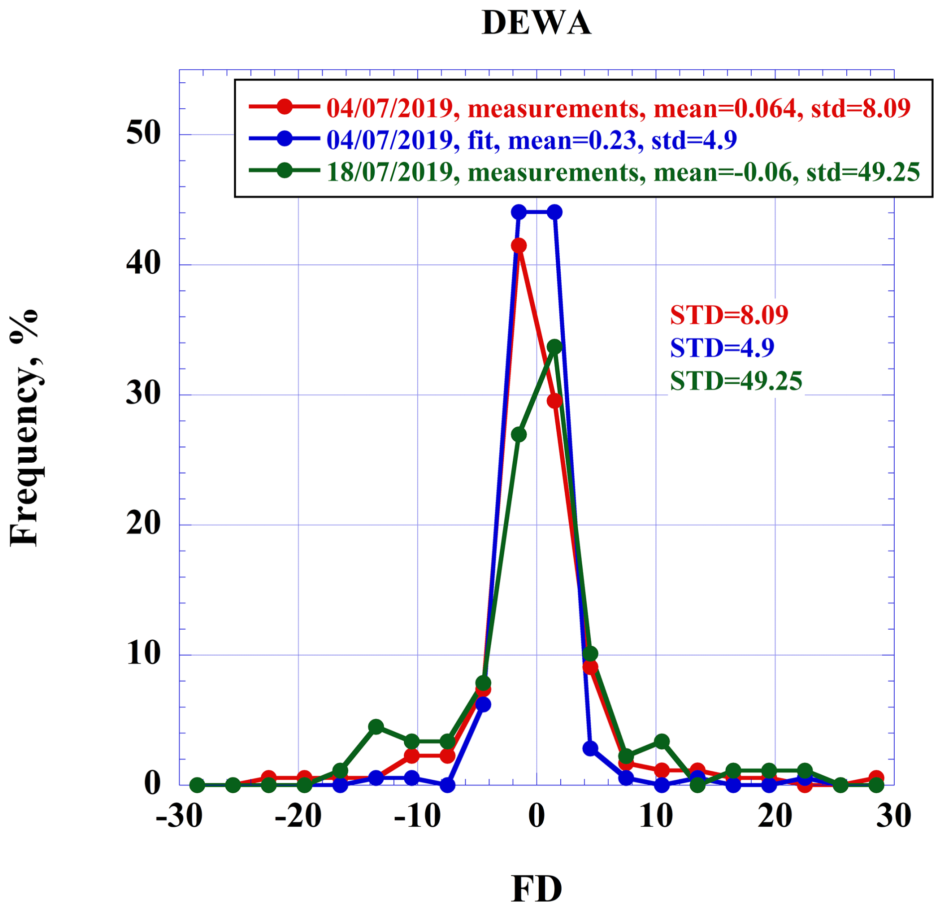
Figure 7 Distributions of FD calculated from CCS measurements at DEWA AERONET site: 4 July 2019 (cloud free conditions), Fig. 4b (red line), polynomial fit to these measurements Fig. 4b (blue line), 18 July 2019 (partial cloudy day), Fig. 5.

The Ilorin case of Fig. 4a is an example of when the algorithm stops after the first iteration because STD starts increasing by removing random spikes due to aerosol. Figure 8a shows an example of CCS (3.3) temporal dependence measured at the Kuopio site (Finland) where it is completely dominated by clouds with no visible aerosol signature. In this case the algorithm also stops after the first iteration. Therefore, the most favorable condition for FD algorithm successful performance is partial cloud contamination throughout the day when an aerosol temporal signature is present. In cases similar to Ilorin (Fig. 4a) the algorithm will keep the aerosol AOD data intact, but for cases like Kuopio it is out of algorithm applicability. Note that the Kuopio case is also completely cloud screened by the current Version 3 algorithm.

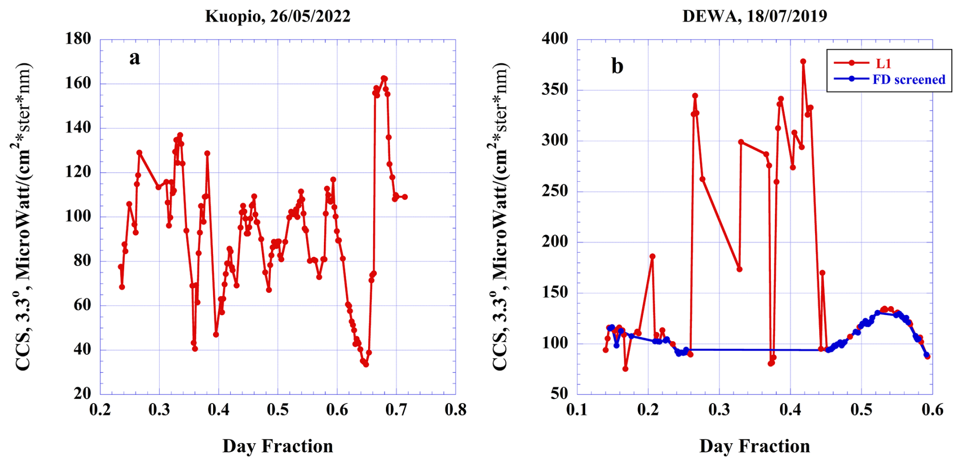
Figure 8 Temporal dependence of CCS (3.3) measured at Kuopio AERONET site on 2 May (a) and at DEWA AERONET site on 18 July 2019 (b).

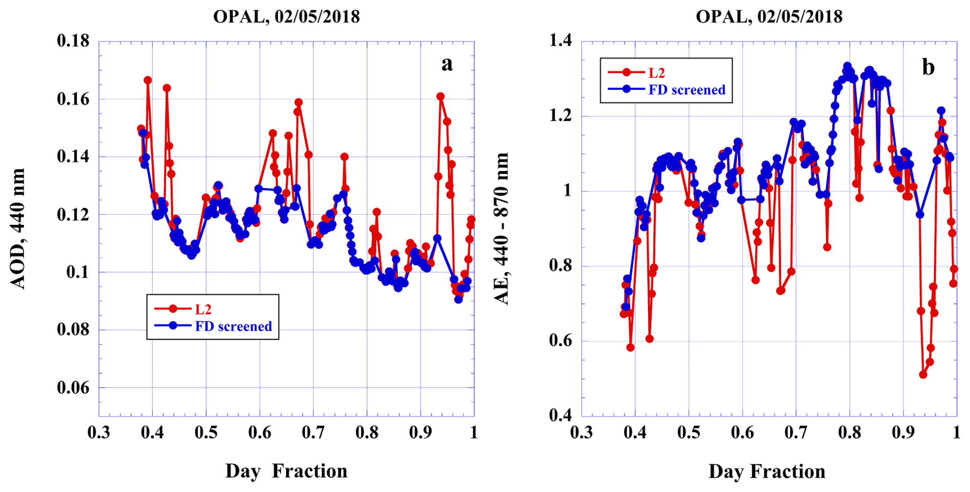
Figure 9 Results of applying of FD algorithm at OPAL AERONET site on 2 May 2018: (a) AOD, (b) AE (440–870).

The FD algorithm was applied to the DEWA case on 18 July 2019 (Fig. 5), and the results are shown in Fig. 8b. For this test the threshold for FD standard deviation was set at 3.0 and was selected from CCS (3.3) temporal dependence measured on a set of cloudless days. Figure 8b shows that application of the algorithm removes irregular spikes associated with clouds and at the same time keeps the smooth part of the temporal CCS (3.3) dependence mostly intact. Figure 9 shows temporal dependencies of AOD (a) and AE (b) for the OPAL site case (Fig. 3) after the FD algorithm was applied. It removes the majority of the upward spikes in AOD and downward spikes in AE associated with clouds. These initial tests illustrate a satisfactory performance of the FD algorithm. However, further adjustments of the threshold value might be needed and adjusted by applying the algorithm to more cases and also subsequent comparison to results of independent cloud detection.

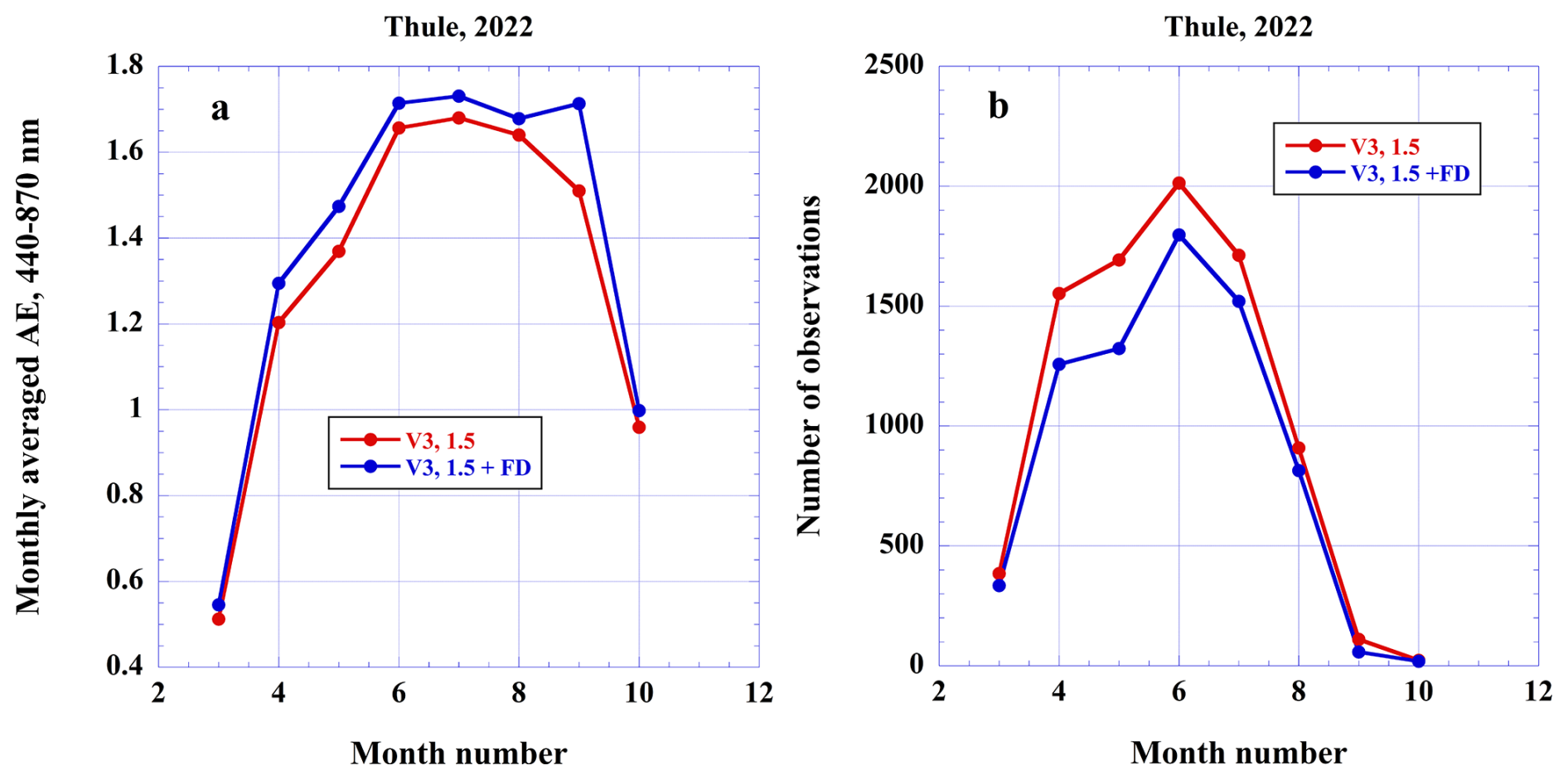
Figure 10 Monthly averaged AE as function of month for Thule AERONET site. Red line corresponds to V3 level 1.5 and blue line after FD algorithm was applied; (a) monthly averaged AE, (b) number of observations.

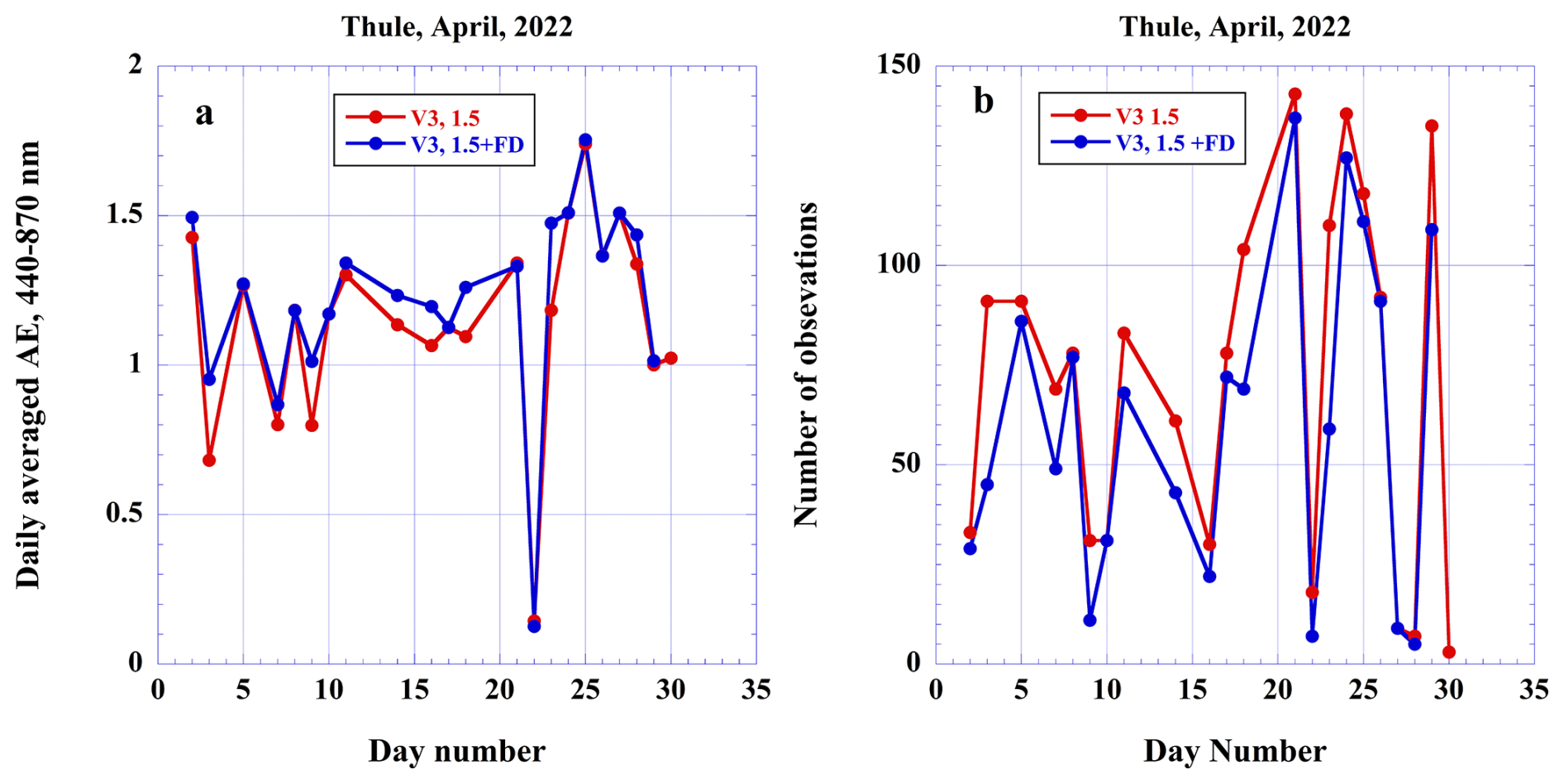
Figure 11 Daily averaged AE as function of day number for Thule AERONET site in April 2022. Red line corresponds to V3 level 1.5 and blue line after FD algorithm was applied: (a) daily averaged AE, (b) number of observations.

5 Algorithm applications at selected AERONET sites

The FD algorithm was applied to the measurements taken at all the AERONET sites in the year 2022. It was found that stand alone performance of FD algorithm, applied to Level 1 (non-cloud-screened data), is less satisfactory than that of cloud screening algorithm of Version 3. However, if applied to Version 3 cloud screened Level 1.5 data, the FD algorithm can identify clouds that were missed by the V3 cloud screening algorithm. Below we present results of applications of the FD algorithm to several AERONET sites. Algorithm performance in the terms of net change in AE and number of observations is analyzed.

Figure 10 shows monthly average AE (a) and number of AOD measurements (b) as a function of month number for the Thule (Greenland) AERONET site. The two curves in each graph correspond to V3 L1.5 (red) and AE averaged values after applying FD algorithm (blue). It should be noted that L1.5 is different from L1.5V which combines cloud-screening and quality assurance (QA) screening as described in Giles et al. (2019). The main feature of Fig. 10a is an increase in AE for all of the months after the FD algorithm was applied which is indicative of the removal of large scattering particles, such as water droplets or ice crystals in clouds. At the same time Fig. 10b shows significant reductions in the number of AOD measurements after the FD algorithm was applied, which is especially noticeable for April, May and June. Figure 11 shows daily average AE (a) and the number of AOD measurements (b) for April. Comparison of Fig. 11a and b shows strong correlation between increases in AE and decreases in the number of AOD measurements which is qualitatively consistent with what is expected after clouds removal. Similar analysis for May and June (not shown) also demonstrated strong correlation between increasing AE and decreasing number of AOD observations. Figure 12 shows analysis of monthly averaged AE and the number of AOD measurements at Hokkaido University, Japan for the year 2022. As in the Thule case, application of the FD algorithm resulted in increasing in AE for all months and reduction in the number of AOD measurements. Additional analysis for April, May and June showed strong anti-correlation between variability of daily averaged AE and the number of AOD measurements.

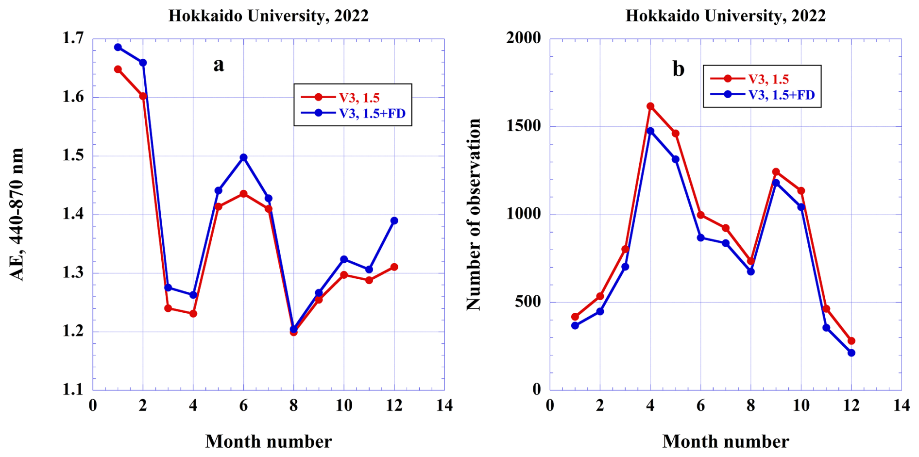
Figure 12 Monthly averaged AE as function of month for Hokkaido University AERONET site. Red line corresponds to V3 level 1.5 and blue line after FD algorithm was applied: (a) monthly averaged AE (440–870), (b) number of observations.

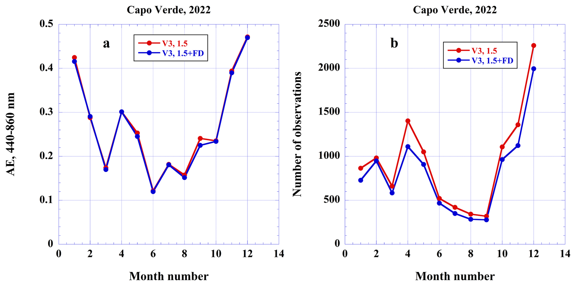
Figure 13 Monthly averaged AE as function of month for Capo Verde AERONET site. Red line corresponds to V3 level 1.5 and blue line after FD algorithm was applied: (a) monthly averaged AE (440–870), (b) number of observations.

Figure 13 shows monthly average AE (a) and number of AOD measurements (b) for the Capo Verde site with aerosol loading dominated by transported desert dust. In contrast to the Thule and Hokkaido University cases, very small changes in AE are accompanied by substantial reductions in the number of AOD measurements. Figure 14 shows daily average AE and the number of AOD measurements for the month of April for which the reduction in the number of measurements is the largest of all the other months. As can be seen, these is no obvious correlation between changes in AE and the reduction in the number of measurements meaning that the FD algorithm removes cloud free observations at this site. In the dust aerosol case, the aerosol/clouds separation becomes very challenging. In the particular case considered (Fig. 14a), the AE during algorithm iteration stays practically constant. In addition, inspection of 3.3° radiances diurnal variability for this day is relatively smooth and does not exhibit any sharp features. Therefore, it was concluded that in this case the algorithm was removing aerosols and was considered algorithm failure. For better understanding of the FD algorithm performance in the Capo Verde case, it might be helpful to analyze the rate of change in AE as the FD algorithm iterations proceed. Figure 15 shows the histograms, based on the data from the entire year of 2022, of the difference between AE of V3 L1.5 and AE after the FD was applied after first (a), second (b) and third (c) iterations. In addition, each graph displays histograms of the relative difference between the number of measurements corresponding to V3 L1.5 and after the FD algorithm was applied. Figure 15a shows that after the first iteration, the maximum change in AE is around −0.006 and the reduction in number of measurements at a maximum of ∼ 15 %. The AE difference variability within the peak is ∼ 0.01 while the total reduction in the number of measurements is about 60 % which is obtained by summing the histogram points corresponding to the relative decrease in the AOD measurements number within AE difference peak. This is a very small change in AE for a rather large change in the number of observations. With the increase in the number of iterations, the maximum peak of AE difference is shifting in the direction of negative values of −0.006, −0.0045, −0.01 with maximum negative AE difference at 10 % level of y axis of −0.009, −0.012 and −0.02 after first, second and third iterations respectively.

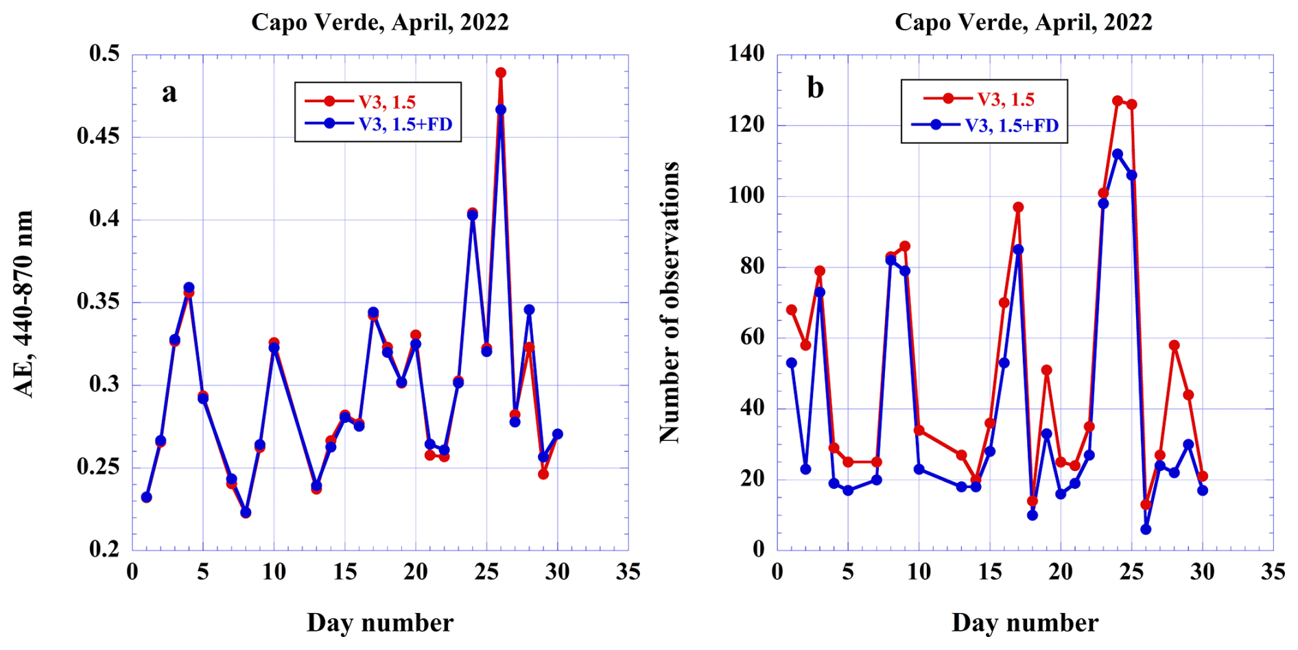
Figure 14 Daily averaged AE as function of day number for Capo Verde AERONET site in April 2022. Red line corresponds to V3 level 1.5 and blue line after FD algorithm was applied: (a) daily AE (440–870), (b) number of observations.

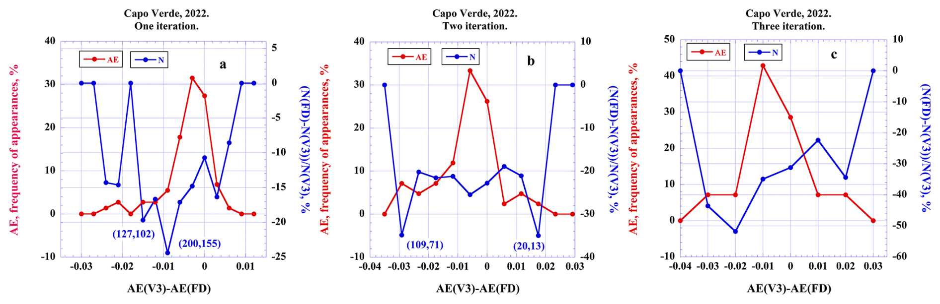
Figure 15 Histograms of the difference between AE corresponding to V3 L1.5 and AE after the first iteration of FD algorithm (red line) as well as relative difference in the number of AOD observations (blue line). Capo Verde AERONET site for the entire year of 2022: (a) after one iteration, (b) after two iterations, (c) after three iterations. The first number in the ordered pair in parentheses is the number of AOD measurements before the iteration and the second number is the one after.

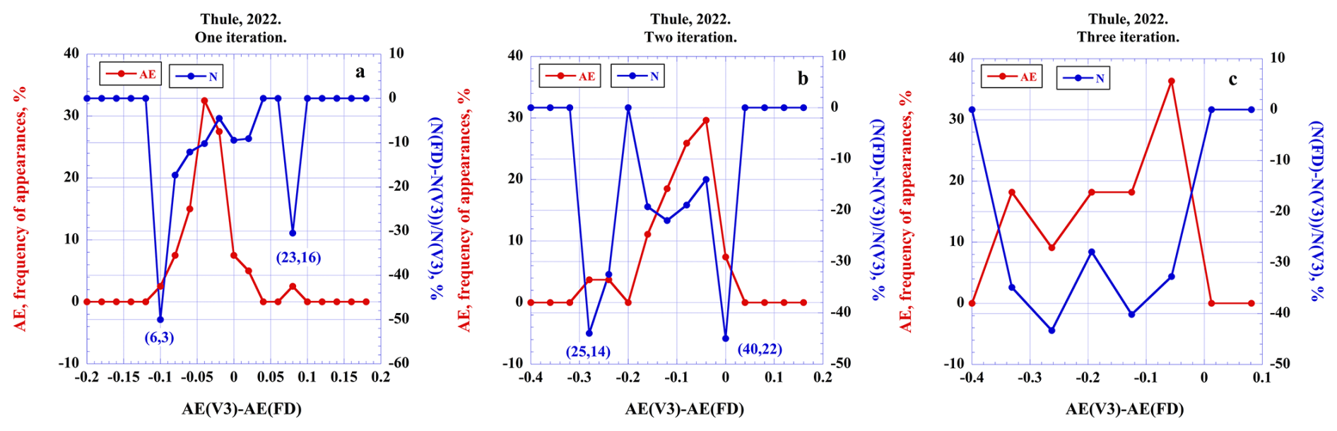
Figure 16 Histograms of the difference between AE corresponding to V3 L1.5 and AE after the first iteration of FD algorithm (red line) as well as relative difference in the number of AOD observations (blue line). Thule AERONET site: (a) after one iteration, (b) after two iterations, (c) after three iterations. The first number in the ordered pair in parentheses is the number of AOD measurements before the iteration and the second number is the one after.

Figure 16 shows a similar analysis for the Thule site data for all of 2022. After the first iteration, the maximum decrease in AE difference is ∼ 0.035 with the reduction in the total number of observations around 10 %. The variability within AE difference peak is ∼ 0.15 while the total reduction in the number of measurements ∼ 75 % as compared to 0.01 (60 %) for Capo Verde. The dynamics of the increase in maximum of AE difference as iteration proceed is ∼ 0.035, 0.04 and 0.06 after the first, second and third iterations respectively. However, due to asymmetry of the maximum AE difference peaks after second and third iterations, the change in AE difference at 10 % of AE difference level to the left is much larger: −0.08, −0.18, and −0.26. The obvious differences between two cases are the different rate of change of AE as iterations proceed. Figure 17 shows the dependence of AE on the number of iterations for 2 April 2022, at the Capo Verde site (a) and 3 April 2022, at Thule (b). In the case of Capo Verde, the linear fit is characterized by low correlation coefficient and very small regression slope. In contrast, for the Thule case, the correlation coefficient is close to one and the regression slope is on order of several magnitudes higher than that for the Capo Verde case. Therefore, the linear regression slope can be used to characterize the rate of change of AE with iteration number. For Capo Verde, the slope is very small in comparison to Thule case where some clouds were removed. This slope value can be used to impose an additional control on the implementation of the FD algorithm. We propose to disregard the FD results if the regression slope is below some threshold. Due to the slope sensitivity to the initial baseline AE, we also explored the option of the AE regression slope after normalization by the first AE value. The results showed that in both cases (Fig. 17) slopes increased after normalization but only slightly: $\mathrm{6.5}\times {\mathrm{10}}^{-\mathrm{5}}$ to $\mathrm{2}\times {\mathrm{10}}^{-\mathrm{4}}$ for Capo Verde and 0.061 to 0.075 for Thule. Therefore, we concluded that normalization of AE would not provide significant improvements in algorithm performance.

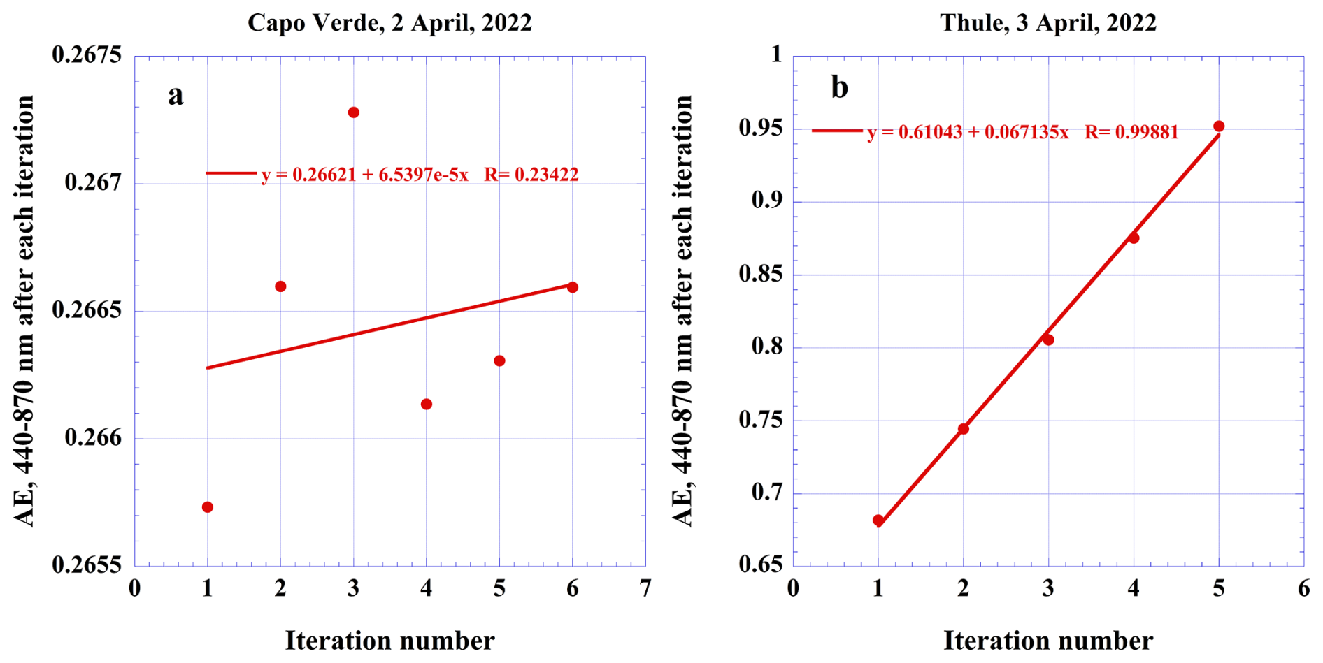
Figure 17 The dependence of net change in AE on the iteration number at (a) Capo Verde AERONET site on 2 April 2022, (b) Thule AERONET site on 3 April 2022.

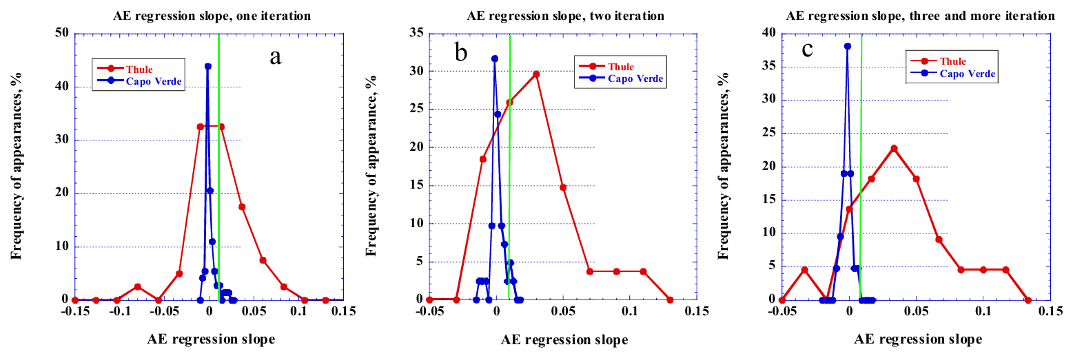
Figure 18 The histograms of AE regression slope after one FD iteration for Thule (red line) and Capo Verde (blue line) for the entire year of 2022: (a) after one iteration, (b) after two iterations, (c) after three and more iterations.

Figure 18 shows histograms of regression slope for Capo Verde (blue line) and Thule (red line) after one (a), two (b) and three iterations (c). The main difference between two cases is that histogram for Capo Verde does not change much with iteration number while histogram for the Thule case is shifting in the direction of larger slopes and becomes wider. As Fig. 18c shows, the upper limit of the histogram for Capo Verde is close to 0.01. This value of the regression slope value could be used as a start value for the threshold to control FD algorithm cloud removal. Figure 19 shows histograms for Capo Verde and Mongu (Zambia) after two FD iterations for the entire year of 2022 data. As can be seen, the histograms for Capo Verde and Mongu are very similar, and the same threshold of regression slope can be applied in both cases. Also, the threshold should be positive because negative value corresponds to decrease of AE after each iteration.

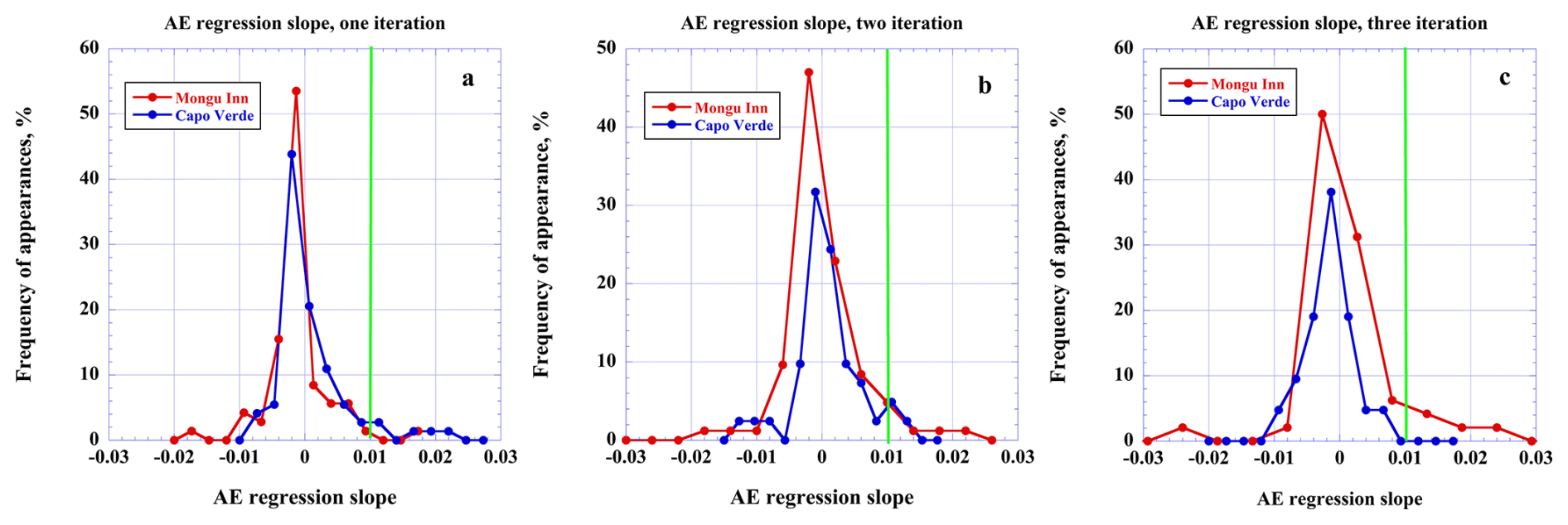
Figure 19 The histograms of AE regression slope after one FD iteration for Mongu Inn (red line) and Capo Verde (blue line) for the entire year of 2022: (a) after one iteration, (b) after two iterations, (c) after three iterations.

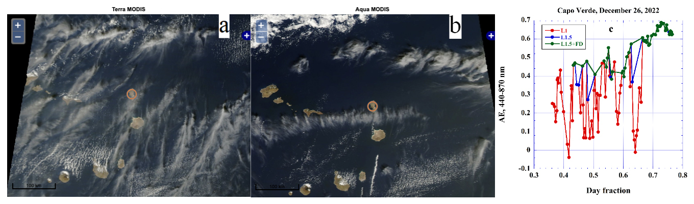
Figure 20 Terra MODIS image of the area in vicinity of the Capo Verde AERONET site on 26 December 2022: Terra (a), Aqua (b), time series of AE, red, blue and green lines depict L1, L1.5 and L1.5 after application of the FD algorithm respectively.

Figures 20, and 21 show examples of application of the FD algorithm to two days at the Capo Verde site: 26 December 2022 (Fig. 20) and 16 November 2022 (Fig. 21). In both cases the FD algorithm was applied without imposing AE regression slope criterion to demonstrate the FD algorithm performance when regression slope is above and below the 0.01 threshold. Figure 20 depicts two MODIS images (Terra, Fig. 20a and Aqua, Fig. 20b) with the Capo Verde site located approximately at the center of each image and the time series of AE (Fig. 20c) with L1, L1.5 and L1.5 plus FD depicted by red, blue and green lines respectively. For this case, the AE regression slope was estimated to be ∼ 0.018 which is above the suggested threshold of 0.01 suggesting some cloud presence. Both MODIS images show some cirrus clouds around the Capo Verde site in each image on 26 December 2022. Applying the FD algorithm resulted in an increase in AE by 0.015 and decrease in AOD at 440 nm by 0.004 (2.7 % from L1.5 AOD ∼ 0.139) and in decrease of the number of observations by 6 from 57 to 51. Figure 20c shows that application of the FD algorithm eliminated some downward spikes in AE time series which are likely due to clouds. Figure 21a and b shows MODIS images and Fig. 21c time series of AE for 16 November 2022. In this case the regression slope was estimated as ∼ 0.0065 therefore being below the 0.01 threshold. Both MODIS images show no or very thin cirrus clouds around the Capo Verde site. In this case applying the FD algorithm resulted in increase in AE by 0.011 and a decrease in AOD at 440 nm by 0.0014 (0.7 % from L1.5 AOD ∼ 0.195) and a reduction in the number of measurements by 29 from 115 to 86. Figure 21c shows that applying the FD algorithm smoothed out the diurnal variability of AE which resulted in an increase of the daily averaged value of AE. However, it is more likely due to elimination of random oscillations of observed AE values due to aerosol and less likely due to clouds. Therefore, imposing a slope of regression check in this case would save ∼ 25 % of mostly cloud free AOD observations.

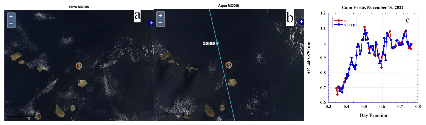
Figure 21 MODIS images of the area in vicinity of the Capo Verde AERONET site on 16 November 2022: Terra (a), Aqua (b), time series of AE, red and blue lines depict V3 and V3 after application of the FD algorithm respectively. On the Aqua image, blue line shows the Aqua MODIS satellite track.

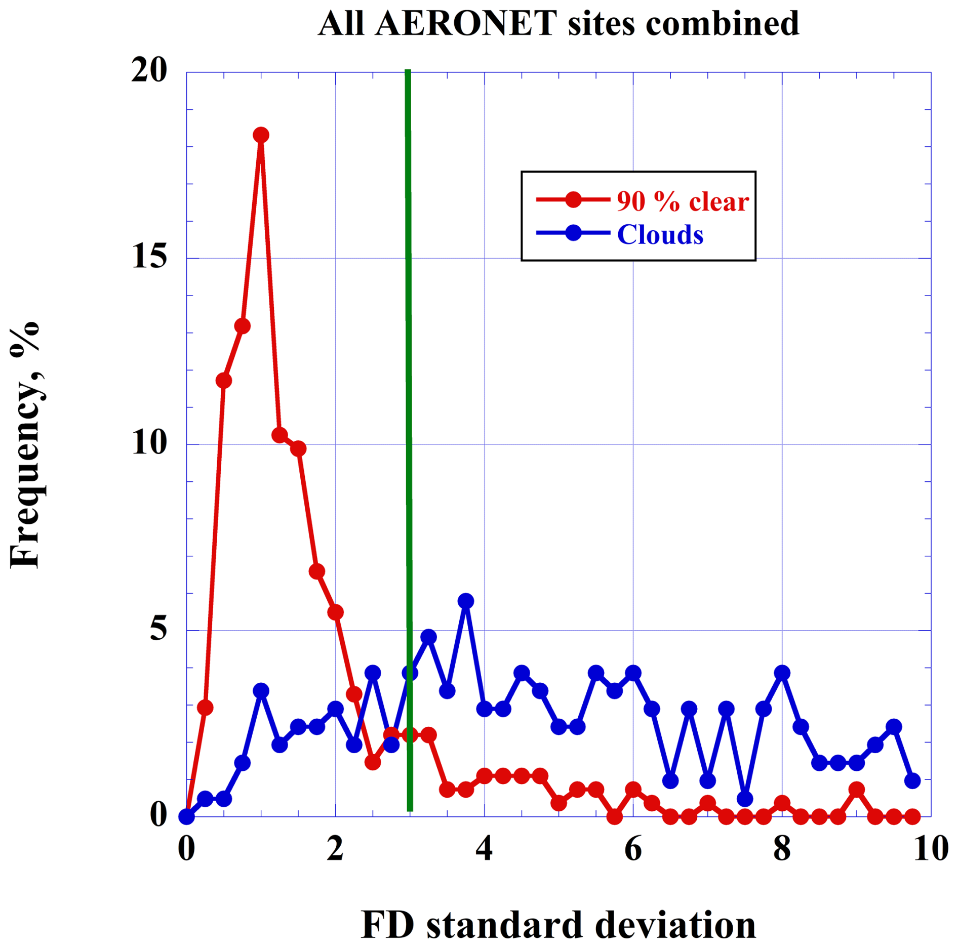
Figure 22 Distribution of FD standard deviation for 90 % clear (red line) and cloudy (blue line) conditions. Vertical line shows selected value for the threshold.

Employing the slope of AE regression as an additional parameter controlling the removal of the AOD data could be considered as an empirical fix in situations when the removal of the large amount of data is in doubt. The rationale for this is the following: one needs to remember that FD algorithm is applied to the results of V3 cloud screening algorithm, which effectively removed the majority of clouds. Therefore, it is assumed that situations with low dynamics of AE variability correspond on average to algorithm failure. The empirical fix will restore the wrongly eliminated data. This is the compromise which was made in situations where separation between large particles and clouds is inheritably difficult.

6 Algorithm validation

Independent cloud detection information from the Micro-Pulse Lidar network (MPLNET) (Campbell et al., 2008; Lewis et al., 2016) was used to both finalize the threshold value for the FD standard deviation and evaluation of FD algorithm performance. MPLNET derives a cloud mask, which provides information on the presence and vertical distribution of clouds. Using vertically resolved lidar backscatter profiles, these datasets identify cloud layers, classify clear versus cloudy conditions, and estimate cloud base and top heights with high temporal resolution. The cloud mask is derived through automated algorithms that analyze signal strength and uncertainty, and temporal continuity to detect cloud boundaries. These data are essential for studying cloud–aerosol interactions, validating satellite retrievals, and improving radiative transfer and climate models. MPLNET cloud mask is sensitive to cirrus cloud, which can be useful for this study. AERONET and MPLNET data were space and time – collocated to perform inter-comparison and assess the quality of the AERONET cloud masking algorithm. In addition, data were averaged over an hour period from both measurements. The MPLNET data from the following eight AERONET stations were used: GSFC (USA), Barcelona (Spain), El Arenosillo (Spain), EPA-NCU (Taiwan), Kanpur (India), Kuching (South Korea), Santa Cruz Tenerife (Spain), and UH Liberty (USA).

The FD standard deviation was calculated for AERONET observations collocated with MPLNET lidars. For estimating the threshold for FD standard deviation, two classifications were derived using the MPLNET cloud mask: 90 % clear and cloudy, which combined all types of clouds detected by lidar. Figure 22 shows frequency distribution of calculated FD standard deviation matched with these two products and combining data from the eight collocated AERTONET sites. Figure 22 shows that in clear condition FD standard deviation exhibits a sharp increase in the range from 0.5 to ∼ 2.0, with the whole range of variability from zero to up to 10.

In this range, distribution of the FD standard deviation corresponding to cloudy conditions does not exhibit any sharp features and stays below ∼ 5 %. Comparing distributions for clear and cloudy conditions allows selecting the threshold value above which clear distribution is dominant. As can be seen from Fig. 22, the threshold value of 3 can be considered as reasonable value. This value is consistent with the value estimated from individual cloud free cases analyzed independent of lidar data.

Figure 23 shows the comparison between the AERONET Version 3 Level 1.5 (V3_L1.5) and the FD (abbreviated as New CS) algorithms across eight co-located AERONET–MPLNET sites as a function of Matthews Correlation Coefficient (MCC). MCC is a is a tool for model evaluation. It measures the differences between actual values and predicted values and is equivalent to the chi square statistics for a 2 by 2 contingency tables (Kaden et al., 2014). The coefficient takes into account true negatives, true positives, false negatives and false positives. This reliable measure produces high scores only if the prediction returns good rates for all four of these categories (Chicco and Jurman, 2020). For each site, data were analyzed under three maximum solar zenith angle (SZA) thresholds – 30, 60, and 90° – to assess how solar geometry affects the agreement between the two cloud screening methods. On average, the FD algorithm outperformed V3 L1.5 by about 0.02 in MCC, suggesting a modest but consistent improvement in overall classification accuracy. Both algorithms exhibited an average decline in MCC with increasing SZA – from about 0.54 at 30° to 0.52 at 90° – indicating reduced comparability at larger zenith angles. This reduction in correlation is mostly due to the lidar pointing straight up (the equivalent to 0° SZA for the sun photometer) while the Cimel is pointing towards the horizon at larger SZAs therefore the two sensors may be detecting different cloud presence due to the spatial variability of clouds in the sky. Despite this degradation, the FD algorithm maintained superior performance across all angles, showing enhanced ability to identify cloud-contaminated observations while retaining a strong balance between detection and rejection. These results suggest that the FD algorithm provides a more refined and reliable screening approach, particularly under favorable illumination conditions, and holds potential for broader application in improving AERONET–MPLNET data synergy and aerosol product quality.

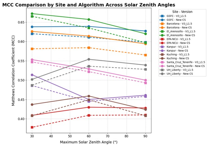
Figure 23 Dependence of Matthews correlation coefficient (MCC) on the maximum solar zenith angle for V3 Level 1.5 cloud screened data and data additionally screened FD algorithm abbreviated here as New CS.

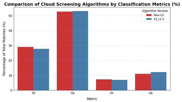
Figure 24 Comparison of V3 Level 1.5 cloud screening results with those of FD (New CS) in terms of the MMC metrics.

Figure 24 compares FD and V3 L1.5 algorithms performance in terms of MCC metrics. The metrics included true positives (TP), true negatives (TN), false positives (FP), false negatives (FN), and MCC, which provides a balanced measure of classification quality. Overall, the FD algorithm achieved higher TP and slightly higher FP counts, indicating a more assertive cloud identification approach, while maintaining better MCC values than V3_L1.5 across all SZAs. The comparison of cloud-screening algorithms reveals that the FD cloud screening method outperforms AERONET V3 L1.5 overall. The FD identifies a higher percentage of true positives and fewer false negatives, indicating improved cloud detection accuracy. While it produces slightly more false positives, the increase is modest and outweighed by its stronger detection sensitivity. Both algorithms maintain high true negative rates, reflecting reliable, clear-sky identification. Overall, the FD algorithm achieves a more balanced and accurate classification, consistent with its higher MCC values across solar zenith angles.

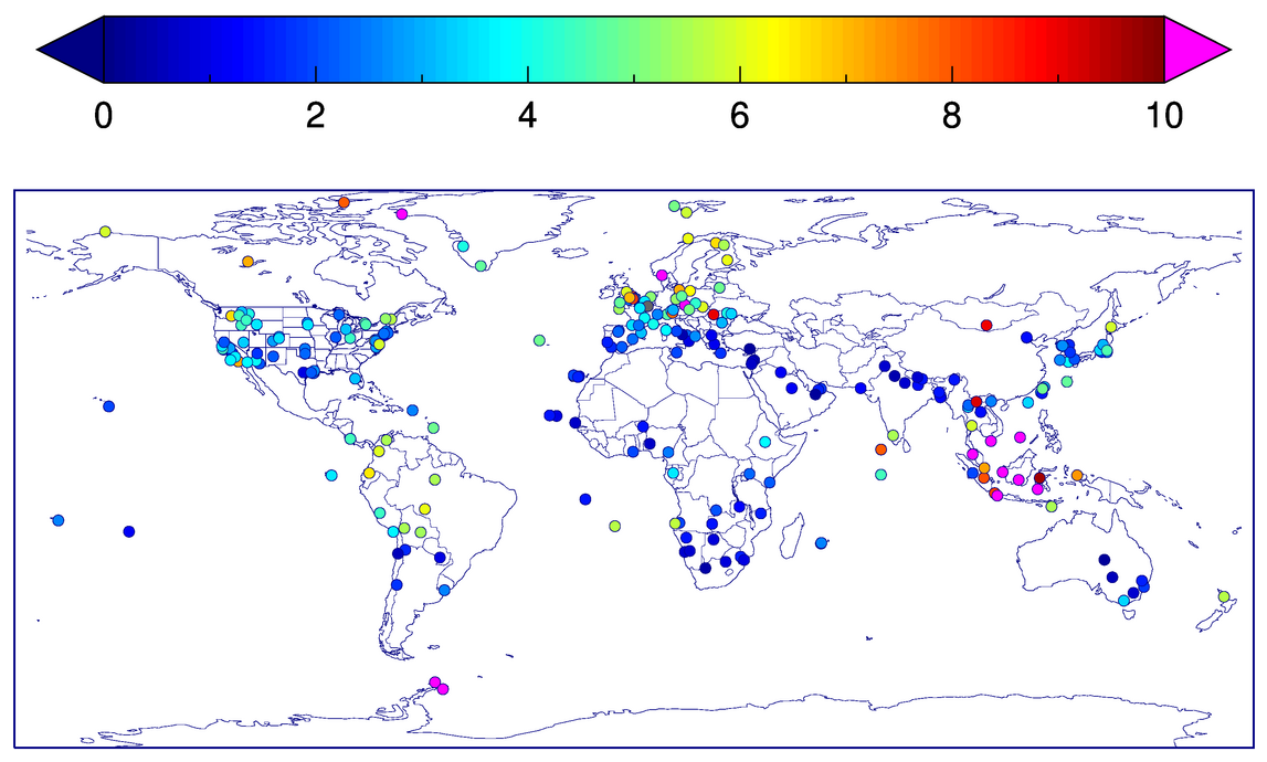
Figure 25 The percentage of data points which did not pass the FD test from V3 L1.5.

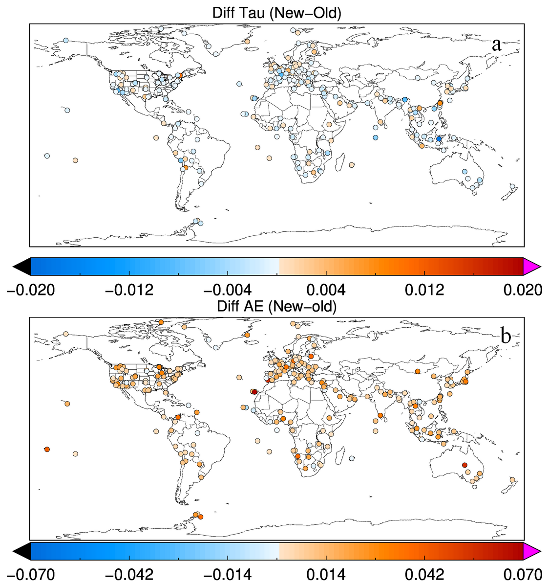
Figure 26 Percentage changes in AOD (a) and AE (b) due to the FD algorithm application. Positive: increased after applying the FD test, negative: decrease after applying the FD test.

The net change in MCC can be put in context of both the number of additional removals of AOD measurements by FD algorithm and the net changes in average AOD and AE. In general, the number of additional removals will vary geographically. Figure 25 shows the geographical distribution of the percentage of data points which did not pass the FD test from V3 L1.5 with an average number of about 3.1 %. Because the FD algorithm is after that of V3 which has already removed the majority of the clouds, even small percentages of additional cloud removal globally or regionally are significant especially in the context of field campaigns or investigations involving limited number of days of sites located in regions with high cirrus cloud fractions. The magnitude of the net changes in AOD and AE depends on the size of the data set analyzed. However, changes in the average AOD and AE are not good metrics for evaluating the FD performance. The FD, being an addition to the V3 cloud screening algorithm, removes relatively small number of AOD measurements to significantly affect the AOD and AE. For example, for Barcelona data set corresponding to the 30 degrees SZA, MCC increase of 0.045 does not correspond to any changes in AE and AOD due to only 6 % increase in TP. Figure 26 shows the geographical distribution of AOD and AE changes due to FD application. The net changes in MCC values should be analyzed considering all the four categories contributing to MCC although the two most important are TP and FN whose variability primarily determines the value of MCC. For example, in the Barcelona case, MCC increase by 0.05 corresponds to the increase of the TP of 9.7 % and decrease of the F N by 12.8 %.

7 Summary and conclusions

A new cloud screening technique augmenting the V3 cloud screening algorithm is presented and discussed. It utilizs the smoothness of diurnal variability of sky radiances measured in the aureole by the CCS scan at 3.3° scattering angle: smooth dependence considered representative of cloud free conditions and sharp spikes are indicative of cloud presence. The technique works best for partially cloudy days when smooth aerosol signature is interrupted by spikes due to clouds presence. The addition of the new technique improves performance of the V3 curvature algorithm in cases when its parameters are below or above corresponding thresholds.

The review of the V3 curvature algorithm is presented and its shortcomings are analyzed. The curvature algorithm allows fully automatic cloud screening procedure and employs two parameters to determine cloud presence: slope of the curvature and curvature calculated at the smallest scattering angle (named the first point) with thresholds for these parameters determined from space and time collocated lidar data. The analysis showed that the curvature algorithm fails cloud detection in cases with curvature slope values below or the first point values above the corresponding threshold values especially at northern latitudes where the size of ice crystals in cirrus clouds are small and comparable with size of aerosols. It is concluded that additional information is needed to improve algorithm performance.

The analysis of diurnal variability of the curvature slope and the first point at the OPAL station in the Canadian high arctic (latitude ∼ 80° N) where majority of the clouds were not detected because both parameters were below (slope) or above (first point) of the corresponding thresholds, demonstrated non-smooth behavior due to the spikes associated with clouds. Similar non-smooth smooth diurnal variability is observed for AE. Therefore, the non-smoothness of temporal variability of curvature parameters as well as AE could be used for cloud detection. However, both curvature parameters are derived from measurements of sky radiances and subjected to constraints such as measurement noise and AOD level. Therefore, it is preferable to use temporal variability of measurements themselves such CCS scan at the second smallest scattering angle (3.3°). The smallest scattering angle (3°) is excluded due to possible stray light effect. Analysis of diurnal variability of CCS(3.3) sky radiances at cloud free conditions demonstrated a smooth dependence that could be approximated by polynomial fit with high correlation coefficients. The common feature in these cases is the presence of a rather smooth temporal aerosol signature interposed by random noise due to the natural variability of aerosols. Another example at the DEWA site in the United Arab Emirates (latitude ∼ 25° N) demonstrated two main features of the temporal variability: smooth part due to aerosols and irregular spikes due to clouds. The main idea of the algorithm is to remove spikes associated with clouds (and associated AODs), while keeping the smooth part intact.

The identification of spikes in time series of CCS (3.3) is done by comparing the magnitude of the sky radiances at neighboring time stamps. Technically it is done by calculating the first differences (FD) of measured sky radiances. Then the standard deviation of FDs for the entire day is calculated and compared to the threshold determined from diurnal dependencies of sky radiances measured on the set of cloud free days. If the standard deviation is larger than the threshold the algorithm marks all the FD pairs above the threshold as cloud contaminated. For those pairs, the algorithm removes measurements of AOD corresponding to CCS (3.3) with the largest magnitude in each pair thereby producing the first iteration “cloud screened” time series for which a new value standard deviation is calculated. The algorithm then proceeds in iterations until the standard deviation is below the threshold or until standard deviation starts increasing. Increasing the standard deviation indicates that the algorithm starts eliminating random variability which can be due to aerosol inhomogeneity or completely cloudy conditions with no clear aerosol signature. The latter case is out of algorithm applicability, and it stops after the first iteration.

The FD algorithm was applied to the measurements taken at all the AERONET sites in year 2022 that had L1.5 data. It was found that stand alone performance of FD algorithm is less satisfactory than that of the curvature algorithm of the V3. However, if applied to the V3 L 1.5 data, the FD algorithm can identify clouds that were missed by the V3 curvature algorithm. The application of the FD algorithm to several AERONET sites is presented and its performance was analyzed in terms of the net change in AE and the number of AOD measurements. It was found that at AERONET sites dominated by fine mode aerosols (Opal, Thule, Hokkaido University), application of the FD algorithm resulted in a systematic increase of the monthly averaged AE as well as the reduction of the number of measurements with AE increase strongly correlated with the decrease in the AOD measurements number. This anticorrelation can be considered as an indication of satisfactory FD algorithm performance at these sites. However, at the Capo Verde site, where aerosol loading is dominated by transported dust, the FD algorithm resulted in a significant reduction in the number of AOD measurements that corresponded to very small changes in AE with no obvious correlation thereby indicating removal cloud free AOD measurements. An additional analysis showed that in cases of remove of cloud contaminated and cloud-free AOD measurements the rate of AE change with iteration number is very different. It is higher for cloudy conditions with linear dependence of AE on the iteration number and it is much lower for cloud free condition with very low correlation between changes in AE and iteration number. The slope of linear regression between iteration number and AE is selected as an additional constraint on the FD algorithm performance. It was decided to disregard FD algorithm results if the slope is smaller than certain threshold value. Based on comparison of FD algorithm dynamics for cloudy and cloud free cases, the threshold value for the slope was selected to be 0.01. The choice was additionally validated by analyzing two days of measurements at the Capo Verde site using MODIS Terra and Aqua images as independent information of cloud presence in the vicinity of the site.

Finalization of the FD algorithm threshold setting as well as evaluation of the algorithm performance was done by using independent cloud detection information available from MPLNET data. AERONET and MPLNET data were space and time collocated, and, in addition, data were averaged over an hour period from both measurements. For finalizing the threshold for the FD standard deviation, two classifications were derived from the MPLNET data product: 90 % clear and cloudy. The FD standard deviation was calculated for AERONET/MPLNET collocated data for both products, and the threshold value was derived from comparison of the corresponding FDs histograms. The determined value of 3.0 was consistent with the value determined earlier from a set of case studies of cloud free diurnal dependencies of CCS(3.3).

The FD algorithm performance was analyzed by comparing both V3 L1.5 and the FD algorithms results to collocated SZAMPLNET data in terms of the Matthews Correlation Coefficient (MCC). MCC measures the differences between actual values and predicted values and takes into account true negatives, true positives, false negatives and false positives and produces high scores only if the prediction returns good rates for all four of these categories. The collocated data were analyzed under three maximum solar zenith angles (SZA) thresholds – 30°, 60°, and 90. The comparison showed that, on average, the addition of FD algorithm outperformed V3 L1.5 alone by about 0.02 in MCC, suggesting consistent improvement in overall cloud detection accuracy. It is also found that both algorithms show a decrease in MCC with increasing SZA with the FD algorithm, however, maintaining superior performance across all angles. These results suggest that the FD algorithm combined with the V3 cloud screening provides a more refined and reliable screening approach.

Additionally, the FD and V3 L1.5 algorithms performance was analyzed in terms of MCC metrics. The comparison demonstrated that the FD identifies a higher percentage of true positives and fewer false negatives, indicating improved cloud detection accuracy. While the FD generates slightly more false positives, the increase is small and outweighed by its stronger detection sensitivity. Both algorithms maintain high true negative rates, reflecting reliable, clear-sky identification. Overall, the FD algorithm combined with V3 clous screening achieves a more balanced and accurate classification versus V3 alone, consistent with its higher MCC values across solar zenith angles.