Satellite-based global monitoring of urban-scale methane emissions

Quantifying and understanding methane emissions of cities are of great importance given their role in current and future mitigation efforts to reduce climate-forcing emissions. However, it remains challenging to routinely and accurately characterize and verify city-scale methane emission inventories. Although previous studies of urban methane emissions have employed a range of emission quantification methods, a simple, efficient, and widely applicable framework for quantifying urban-scale emissions remains lacking. In this study, we describe our development of an advanced mass balance emissions accounting using TROPOspheric Monitoring Instrument (TROPOMI) satellite observations to estimate the orbit-level net bulk (city-level) methane emissions and corresponding emissions uncertainties due to the method. We have tested and demonstrated that the novel integration of hourly-resolved wind data under the planetary boundary layer (PBL) enables a more conceptually-accurate assessment of methane emissions from urban areas than methods that do not consider thermodynamic variability. In addition, we have introduced an upwind-based approach for background determination, in which background methane concentrations were defined using city-adjacent regions along the PBL-pressure-weighted-mean upwind direction. Initial assessments with this approach were tested for three megacities (London, Los Angeles and New York) between 2021 and 2023. Results indicate that existing emission inventories generally underestimate urban methane emissions across all three cities, but with significant inter-annual and inter-city variability. Satellite-derived emissions from 2021 to 2023 range from 5.99 to 11.90 t h⁻¹ in London, 26.21 to 62.77 t h⁻¹ in Los Angeles, and 30.85 to 44.77 t h⁻¹ in New York, corresponding to factors of approximately 1.5–3.0, 1.3–3.1, and 7.0–10.2 times the inventory estimates, respectively. Compared with previous top-down urban studies for the same cities, our results are generally consistent with the reported emission estimates, with most estimates falling within our uncertainty bounds. These results demonstrate that satellite observations can facilitate ongoing city-scale emission quantification, support inventory reconciliation and reporting, offer the potential for long-term monitoring globally, and further aid efforts to assess whether stated methane emission targets are being met.

1 Introduction

Methane (CH₄), the second most significant anthropogenic greenhouse gas after carbon dioxide (CO₂), is responsible for one third of the rise in global mean surface air temperature from 1750 to 2019 (Szopa et al., 2021). The relatively short atmospheric lifetime (about 9 years; Prather et al., 2012) and substantial global warming potential (almost 82 times that of CO₂ over a 20-year period; IPCC, 2023) make the reduction of methane emissions a compelling strategy for tackling near-term climate change (Forster et al., 2021). All projected pathways for restricting global warming to 1.5 °C above pre-industrial levels need a rapid decrease in methane emissions (IPCC, 2023). Over 150 countries have committed to reducing their methane emissions across all sectors by a minimum of 30 % below 2020 levels by 2030, via their respective Nationally Determined Contributions to the Paris Agreement and the Global Methane Pledge (Global Methane Pledge, 2023).

Methane is released through many natural (e.g., wetlands, inland freshwaters, etc.) and anthropogenic processes, but about 65 % (range of 63 %–68 %) of it originates from human activities, which include agriculture, waste management, and fossil fuel production and use (Saunois et al., 2025). Large emission uncertainties (between 20 %–35 %) have been identified across these sectors in terms of average annual magnitudes and trends among different global bottom-up inventories (Saunois et al., 2025; Tibrewal et al., 2024). These disagreements primarily arise from differences in input data (e.g., activity data and emission factors), as well as variations in sectoral coverage and times-series gap-filling strategies (Saunois et al., 2017; Tibrewal et al., 2024). Urban areas are large and spatially-concentrated methane emission sources, which may impede climate goals, given the prevalent use of natural gas (He et al., 2019), pipeline gas leaks due to aging infrastructure (Weller et al., 2020), and wastewater treatment systems (Defratyka et al., 2021). Field studies quantifying methane emissions in urban areas have found that official bottom-up inventories can underestimate methane emissions by a factor of 2 to 3 (Anderson et al., 2021; Pitt et al., 2022; Plant et al., 2019). Such discrepancies imply that there are substantial unexplained urban sources of methane (Saint-Vincent and Pekney, 2019). Monitoring and mitigation efforts are urgently required, as more than half of the global population already resides in urban areas; this proportion is projected to rise to 70 % by 2050 (United Nations Department of Economic and Social Affairs, 2025), which is expected to exacerbate landfill and wastewater emissions (U.S. Environmental Protection Agency, 2019).

Top-down (measurement-led) quantification methods can evaluate emissions in urban areas from unidentified or underestimated sources, in contrast to bottom-up inventories, which rely on activity data and emission factors that are often difficult to define accurately. Many top-down studies have employed in situ observations (Schiferl et al., 2025), mobile and vehicle ground monitors (Maazallahi et al., 2020), or aircraft (Allen et al., 2019; Pitt et al., 2022) to infer total methane emissions in urban regions. These approaches can deliver accurate emissions snapshots, but cannot deliver continuous temporal monitoring and may have restricted spatial sensitivity. Considering the spatial extent of urban area methane emissions across nations and globally, satellite-based instruments with high spatial resolution have been shown to have the potential to provide implementable monitoring solutions (Cooper et al., 2022; Shen et al., 2023; Vanselow et al., 2024). In 2023, de Foy et al. (2023) demonstrated that satellite column concentration from TROPOspheric Monitoring Instrument (TROPOMI) can be used to constrain current urban-scale methane inventories based on significant methane enhancements over 61 urban areas worldwide. More recently, Nesser et al. (2024) used TROPOMI data to conduct a preliminary national analysis of urban methane emissions across North America (focusing on the contiguous U.S.). However, urban methane emissions are often characterized by a total (yet ambiguous) uncertainty in prior literature, without detailed error-propagation information. Moreover, the inferred emission distributions, which depend on the characteristics of the atmospheric transport models used in different inversion systems, are not typically consistent across satellite-based and surface-measurement-based studies (Saunois et al., 2025). In poorly observed regions (e.g. India, China), where most of the global population resides, measurement-led validation of national emissions is even more challenging. This highlights the need to develop more improved methods with greater transparency in uncertainty budgeting, in order to provide simpler, more conceptually-accurate, and more reliable urban-scale emission estimates than the conventional source pixel method, while remaining globally implementable.

In this study, we present and test new developments to the source pixel method (Buchwitz et al., 2017; Jacob et al., 2016), which we have used to quantify emissions of methane for three megacities. These developments include an improved quantification of planetary boundary layer (PBL) winds and upwind background concentration used in the method. Such improvements are more conceptually accurate than more simple source pixel methods that are agnostic to upwind background direction and wind representation throughout the depth of the PBL. We analyze single-orbit (Level-2) methane column measurements from TROPOMI to quantify urban methane enhancements relative to an upwind background for three case study cities (London, Los Angeles, and New York) over the period 2021–2023, mapped onto a regular 0.1°×0.1° spatial grid. We then evaluate methane emission rates and forward-propagate systematic emission uncertainty using this improved source pixel method. To test and develop the method, we also investigated its sensitivity to varying meteorological conditions (especially wind vectors), and differences in data coverage over the urban source region.

2 Data and methodology

To detect emission rates in hotspot cities based on TROPOMI methane products, we applied a fast and simple remapping method to achieve a constant spatial resolution (0.1°×0.1°) of TROPOMI atmospheric dry-air methane column mixing ratio (XCH₄), and then we used an improved data-driven source pixel method to further infer the emission rates of urban areas. The technical framework of our study is illustrated in Fig. 1, which shows data selection and pre-conditioning prior to emissions quantification. Section 2.1 describes data products, including satellite retrievals and data pre-processing steps to filter for high-quality observations, winds, inventory repository and our definition of urban spatial boundaries. Section 2.2 describes the remapping process of pixel-heterogeneous Level-2 satellite data to temporally-averaged Level-3 data. Section 2.3 describes the improved source pixel method, which quantifies city-level methane emission rate for each viable (cloud-free) overpass. Section 2.4 describes the detailed uncertainty analysis for city-scale emission quantification, including both single-orbit estimates and multiple-overpass estimates across different timescales.

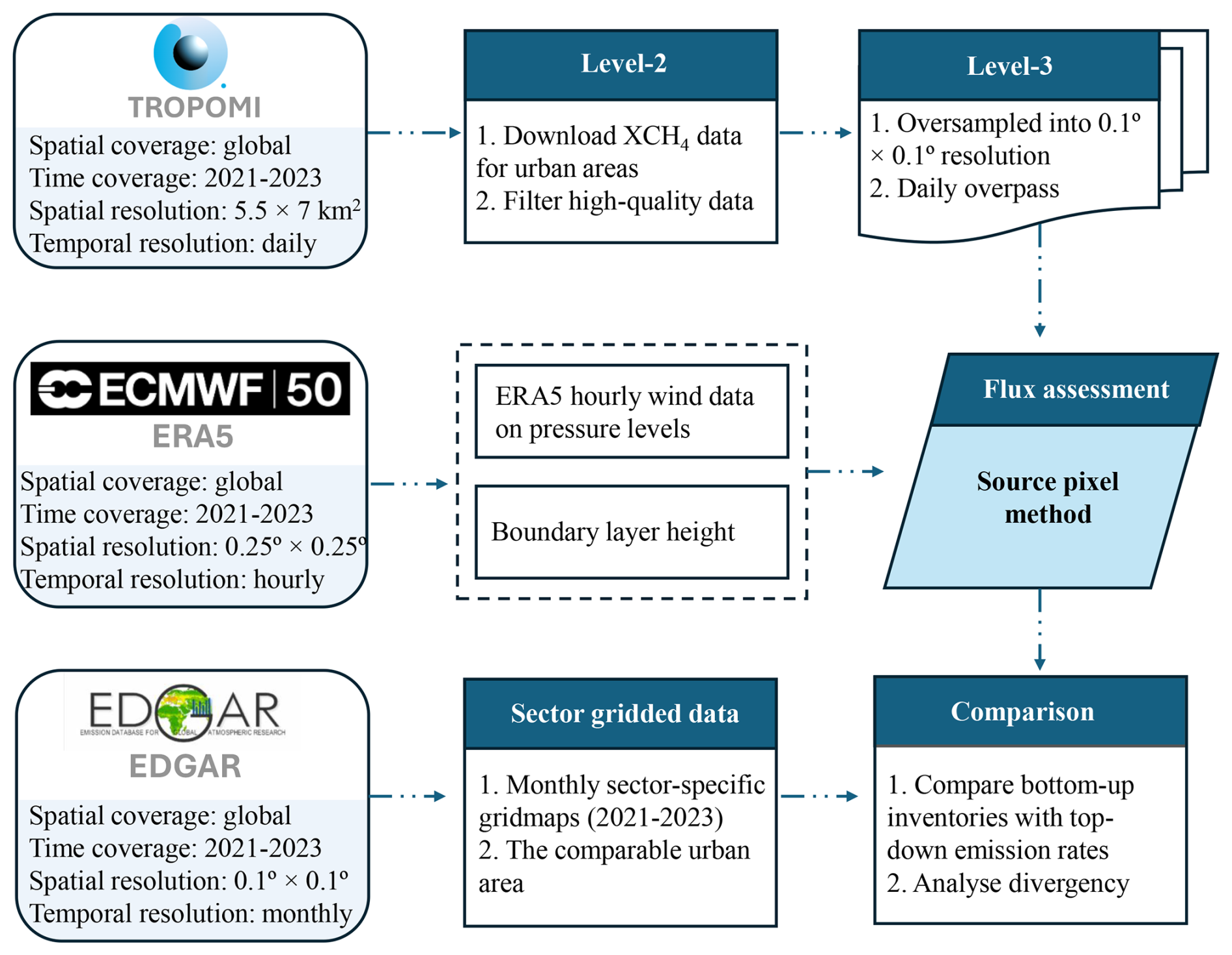
Figure 1 Technique framework of the improved source pixel method designed for urban area methane emissions quantification.

2.1 Data

2.1.1 TROPOMI Satellite retrievals

TROPOMI serves as the only instrument onboard the polar sun-synchronous Sentinel-5 Precursor (S-5P) satellite, launched on 13 October 2017 at an altitude of 824 km, with a consistent 13:30 local overpass time (Veefkind et al., 2012). The instrument retrieves the methane column by detecting solar backscattered light in the shortwave infrared (SWIR) 2.3 µm absorption band with near-uniform sensitivity across the troposphere. XCH₄ is retrieved using a full-physics algorithm under clear-sky conditions, with daily global coverage and spatial resolution of 7×7 km² (7×5.5 km² since August 2019) at nadir (Butz et al., 2011).

In this study, we have used the RemoTeC-S5P operational retrieval product of TROPOMI (Hasekamp et al., 2024). This TROPOMI XCH₄ product was corrected for already known retrieval biases, and validation with independent ground-based measurements from the Total Column Carbon Observing Network showed that the bias-corrected XCH₄ significantly improved the uncorrected product (Hasekamp et al., 2024; Hu et al., 2018). Thus, the corrected column-averaged dry-air mole fraction of methane is used in this study, and obtained at the original swath resolution from 1 January 2021 to 31 December 2023. The retrievals of methane columns achieve an effective success rate of about 3 % of total daytime observations over land (cloud-free measurements), principally constrained by cloud cover, variable topography, heterogeneous albedo of coast pixels and high levels of aerosol scattering (Hasekamp et al., 2024). Thus, we only use good-quality XCH₄ measurements under cloud-free conditions, which we define and filter using the following metadata parameters: qa_value (quality assurance value) > 0.5, solar zenith angle (< 70°), viewing zenith angle (< 60°), and smooth topography (1 standard deviation of surface elevation variability < 80 m within a 5 km radius). Also, pixels with a SWIR aerosol optical thickness > 0.07, or a retrieval precision > 10 ppb were removed. We further screened retrieval data using the surface classification flag recommended by Balasus et al. (2023) and de Foy et al. (2023), keeping only pixels flagged as 0 (land) and 2 (some water), and excluding inland water pixels with poor spectral fits (e.g., with a flag of 2 and SWIR chi-square > 20 000) to remove artifacts. We note that some studies used the well-filtered TROPOMI WFM-DOAS XCH₄ product (Schneising et al., 2023) or blended TROPOMI + GOSAT product (Balasus et al., 2023) that had passed the quality check to estimate emissions of regions (Liu et al., 2024; Wang et al., 2026). But significant differences of XCH₄ retrievals and spatial emission patterns from different products have been identified, which may be attributed to aerosol scattering and sensitivity to albedo (Sicsik-Paré et al., 2026). The operational product used here provides more temporally homogeneous coverage and detailed information about aerosol optical thickness and albedo, which we consider to be the most relevant parameters that may be expected to influence background methane columns, which source pixel methods can be highly sensitive to (see Sect. 2.3).

2.1.2 Wind data

The TROPOMI RemoTeC-S5P data product provides the horizontal components of surface wind at 10 m height, which is derived from the European Center for Medium range Weather Forecasts (ECMWF) and interpolated in space and time to SWIR measurement to calculate the near-surface wind vector of each TROPOMI pixel. In 2019, ECMWF released the latest generation reanalysis model, ERA5, using a four-dimensional variational (4D-VAR) assimilation scheme (Hersbach et al., 2020). For the source pixel method, ERA5 offers significant advantages over 10 m wind in terms of its ability to incorporate u and v wind observations more proximal to time of measurement, and on several pressure levels through the PBL. ERA5 also provides other meteorological variables such as corresponding PBL height and pressure and temperature (from which atmospheric density can be derived). At a spatial resolution of 0.25°×0.25°, ERA5 provides hourly meteorological data, enabling the probability quantification of wind uncertainty (see Sect. 2.4) by incorporating temporal variability in meteorological conditions during satellite overpasses of extensive urban areas. The PBL is the primary layer in which surface emissions are dispersed and advected over urban spatial scales. It is characterized by turbulence and convective mixing, typically mixing throughout the whole layer on timescales of advection across city scales (Pitt et al., 2019). The improved source pixel method is therefore sensitive to prevailing winds throughout the PBL (and not simply 10 m winds), and emission rate is conceptually proportional to mean PBL wind speed (as shown in Sect. 2.3). We therefore calculate total wind for each overpass as the pressure-weighted average of wind speed and direction across all ERA5 PBL pressure levels over a given urban source region, using daily ERA5 PBL height data. Compared with previous studies using prior versions of the source pixel method, we choose here to use the pressure-weighted boundary layer winds instead of 10 m wind provided in the TROPOMI retrieval products, because, conceptually, this better captures the expected ventilation across the source pixel that arises by turbulent horizontal advection in the urban PBL (Pandey et al., 2021; Varon et al., 2018).

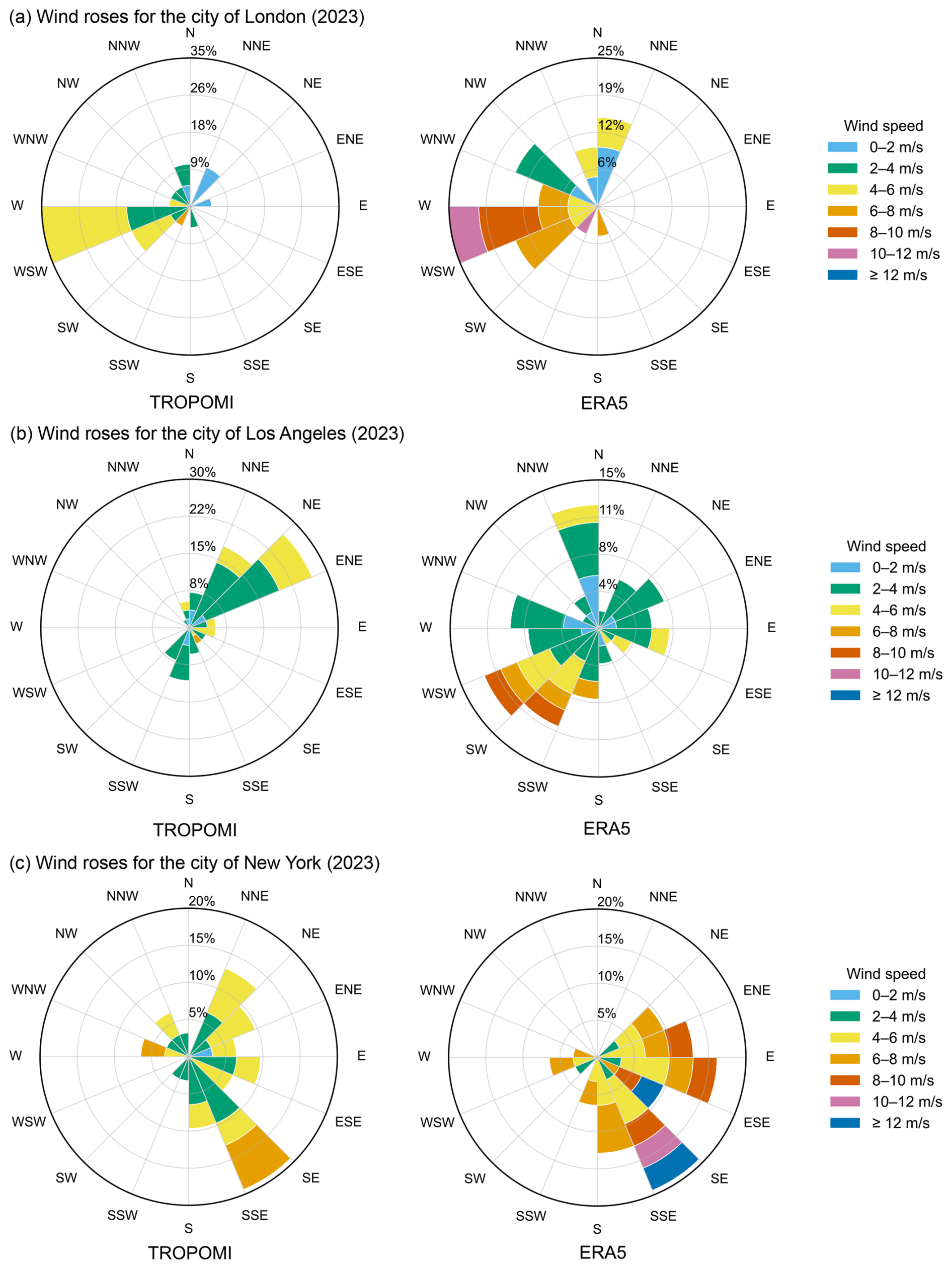
Figure 2 Comparison of wind roses derived from TROPOMI products and ERA5 reanalysis over London (a), Los Angeles (b) and New York (c) for 2023. The annual average wind statistics of each city are calculated using only days with valid TROPOMI overpasses, filtered by all data quality control threshold described in Sect. 2.1.1.

A further comparison of 10 m wind from TROPOMI products and ERA5 data over London, Los Angeles and New York was conducted to assess sensitivity to the choice of winds in the source pixel method in general. Figure 2 indicates that there are significant differences between the 10 m wind and pressure-weighted PBL wind over the source region for the same overpasses. This was a consistent observation in all three cities and influences both the wind speed (that is directly linear to the final methane rate) and the wind direction, which is critical for determining the location of the background region assumed (see Sect. 2.3). In turn, this can affect the magnitude of the methane enhancement, and therefore the calculated emissions. For Los Angeles, most of the time, TROPOMI 10 m wind is from the north-northeast to east-northeast direction and lower than 6 m s⁻¹. But for ERA5 PBL-weighted winds, this is dominated from west-southwest to south-southwest and north to north-northwest, with wind speeds up to ∼ 10 m s⁻¹. Wind direction discrepancies of these two datasets are less significant for London and New York, but all illustrate a higher wind speed in ERA5 (as may be expected). This directly implies a higher emission rate due to the wind ventilation of the source pixel than methods that consider only near-surface wind vector.

2.1.3 Emission inventories

To better understand the nature of any potential discrepancy between bottom-up inventories and top-down measurements, a set of inventories are used for comparison here. The Emissions Database for Global Atmospheric Research (EDGAR v8.0) provides detailed information about anthropogenic emissions of various air pollutants and greenhouse gases (Crippa et al., 2024). EDGAR compiles data from a variety of sources, allowing differentiation between individual sources in a source region. For each sector, annual and gridded emissions are provided from 1970 to 2023 with a spatial resolution of 0.1°×0.1°. This enables us to scale and compare methane emissions in a specified source region with same location and area in EDGAR. Apart from the anthropogenic emissions in EDGAR, the only natural sources of methane included in this study are extracted from WetCHARTs v1.3.3 (Bloom et al., 2024). This dataset was selected because natural wetland emissions constitute the largest and most uncertain component of natural methane sources in bottom-up models and inventories (Saunois et al., 2025).

In addition to EDGAR, gridded methane emission data from the National Atmospheric Emission Inventory (NAEI) for the UK, and the U.S. Environmental Protection Agency (EPA) are also used for comparison. NAEI gives annualized gridded emissions of methane at 1 km × 1 km resolution from 2005 to 2023 and provides sector-specific emissions across the UK (Tsagatakis et al., 2024). The gridded EPA anthropogenic greenhouse gas inventory (GHGI) provides annual methane emissions (0.1°×0.1°) for the contiguous United States (CONUS). The gridded GHGI v2 Express Extension product includes annual emissions from 2012 to 2020 for 27 source categories (Maasakkers et al., 2023). These gridded methane emission products can be used to examine which inventories may perform best and to gain insights on sectors that may dominate uncertainty when compared with the emissions derived in this study at the urban scale.

2.1.4 Choice of urban source domain

Since urban inventories reported for climate change mitigation can be significantly influenced by the choice of city boundary, the cartographic boundary shapefiles of each case study city in this study were obtained from the official website that available to public (City of Los Angeles, 2026; Greater London Authority, 2026; New York State GIS Program Office, 2026). In the process of selecting the urban domain used as the source region in this study, an area was selected as the source region for each study using a square box centered on the mid-points of the maximal meridional and zonal extent of the city's shapefile, oriented such that two sides of the box are perpendicular to the mean PBL wind. This ensures that the full width of the emitted urban plume is observable (in principle) over the city in the TROPOMI scene (assuming cloud-free conditions).

2.2 Remapping method

The pixel size (in terms of ground footprint) during each TROPOMI orbit are different, resulting from changing viewing angles across the swath, and Earth's curvature. In order to map Level-2 pixels to Level-3 grids as a temporal average for use in this work, such that a source region is based on a city boundary shapefile, and directly comparable to gridded bottom-up inventories, we use remapping to generate a regularized grid. Here, we remapped the methane column mixing ratios retrieved from TROPOMI that passed the filters described in Sect. 2.1.1 to a resolution of 0.1°×0.1° for each orbit. Remapping makes use of shifting pixel locations and sizes in daily observations to achieve spatial resolutions finer than the original pixel size. The remapping method treats satellite observation pixels as surface polygons and calculates the fractional area of each grid cell covered by individual pixel polygons. The calculation of this overlapping area requires filling the irregular pixels with regular grid cells, also known as “tessellation”, which is well-described by Zhu et al. (2017). In Zhu et al. (2017), day-to-day observations from multiple overpasses were utilized to oversample satellite column data to increase spatial resolution through temporal averaging. In contrast, in our study, valid pixels from each individual overpass are remapped onto a regular grid to enable orbit-level methane emission estimates. The remapping method is described by the following relationship:

$$\begin{array}{}\text{(1)}& \stackrel{\mathrm{‾}}{\mathrm{\Omega }}\left(i\right)={\displaystyle \frac{{\sum }_{p=\mathrm{1}}^{N\left(i\right)}\frac{A(p,i)}{S\left(p\right)\mathit{\sigma }\left(p\right)}\mathrm{\Omega }\left(p\right)}{{\sum }_{p=\mathrm{1}}^{N\left(i\right)}\frac{A(p,i)}{S\left(p\right)\mathit{\sigma }\left(p\right)}}}\end{array}$$

Where A(p,i) is the overlap area between the pixel p and remapping grid cell i. S(p) is the pixel area. σ(p) denotes the absolute error standard deviation of the satellite observation data as reported in the retrieval products. Ω(p) represents the corrected average total column mixing ratio of methane. Through this remapping method, the area-weighted and error-weighted average column for each 0.1°×0.1° grid cell is then derived. In order to fit to the re-gridded resolution, all variables of TROPOMI retrieval products included in this study were calculated using the same remapping method.

2.3 Emission quantification method

To quantify emissions for each city, the source pixel method that was first introduced by Jacob et al. (2016) is applied here, which was further developed and fully modeled by Buchwitz et al. (2017). This fast data-driven method is derived from the concept of mass balance, and designed to calculate methane surface emissions of areas showing elevated atmospheric concentrations relative to their surrounding areas from satellite retrieval XCH₄ maps. An elegant advantage of the method is that emissions can be inferred solely from methane enhancements (e.g., source minus background value) in the source pixels, along with knowledge of a representative advective flow vector (i.e. mean wind). Source pixel methods usually apply to time-averaged satellite-derived XCH₄ data sets. Despite large systematic emission uncertainties (typically of the order tens of percent), emission uncertainty can be reduced when the signal (over a city) is proportionately larger than the surrounding background area (and when the background is less variable). The source pixel method was used by Buchwitz et al. (2017) to derive urban emissions with magnitudes of several Mt CH₄ yr⁻¹. Here, we propose an improved source pixel method that integrates detailed wind vector information to better represent ventilation over the source region and methane enhancement relative to the upwind background, thereby improving the quantification of city-scale methane emissions.

Detailed application of this improved method in this work is as follows: we first re-grid TROPOMI Level-2 retrieval products using a regular latitude-longitude grid (here: 0.1°×0.1° resolution following remapping as described in Sect. 2.2). The second step defines a source region (SR) and background region (BR) aligned to the mean PBL wind as described in Sect. 2.1.2. Previous applications of the source pixel method assume that the observed methane enhancement in the source area is associated with the source region alone (with no account for the true upwind background) and that any possible enhancement in the background area caused by outflow of the source region can be neglected (Buchwitz et al., 2017). This could bias the estimated methane enhancements and inferred emissions if substantial emissions occur around the source region. Debates remain on the choice of the background domain due to different research scales and locations, including (1) expanding the coordinates of the source region to a size defined by the maximum extents in the meridional and zonal directions (Vanselow et al., 2024), (2) using a large background region to decrease the impacts on emissions estimates from any potential emissions in the background region (Pandey et al., 2021), (3) proposing a land cover weighting method to estimate the background XCH₄ (Xing et al., 2025). An alternative approach to defining a background concentration is to characterize adjacent up-wind regions, though insufficient observations in this region may be caused by clouds, oceans, and other factors affecting retrieval quality can limit the number of days available for emissions analysis. In our variation of the source pixel method, emissions in the background region are implicitly accounted for and subtracted such that the new method does not necessitate the background region to be completely free of methane emission sources. In this work, the background region is defined as an equal area region located upwind of the source region. We chose this novel up-wind method to define the background region located immediately-adjacent and in the upwind direction as defined by PBL-pressure-weighted mean wind as described in Sect. 2.1.2. It is oriented such that two sides of the box (e.g., source region and background region) are perpendicular to the pressure-weighted PBL wind direction, and the full width of the emitted urban plume is observable over the city. The third step calculated the methane enhancement (e.g. ΔXCH₄) for each overpass over the source region compared with its adjacent up-wind background region. This methane enhancement is computed by subtracting the mean retrieved XCH₄ in the background region from the mean over the source region. To minimize potential bias from the statistics of small sampling (and therefore potential bias from outlier pixels remaining after data-filtering), we defined two further thresholds in data coverage that must be met in order for emissions for a city from a single orbit to be considered meaningful, as follows: the source region must be at least 25 % populated with valid data after filtering (Fig. A2). and the background region must have at least 10 observations. This resulted in the loss of the majority of city overpasses (due predominantly to cloudy scenes, in addition to surrounding coasts). We assert that this is an important and necessary loss of data to preserve emissions accuracy. We noted that emissions calculated where we attempted to relax these constraints further, resulted in wildly different and simply impossible results.

Finally, combined with additional TROPOMI retrieval products, the elements extracted above provide all inputs necessary to implement the improved source pixel method and estimate urban methane emission rates:

$$\begin{array}{}\text{(2)}& E={\displaystyle \frac{M_{{\mathrm{CH}}_{\mathrm{4}}}}{M_{\mathrm{air}}}}{\displaystyle \frac{({\mathrm{SR}}_{{\mathrm{CH}}_{\mathrm{4}}}-{\mathrm{BG}}_{{\mathrm{CH}}_{\mathrm{4}}})UPW}{g}}\end{array}$$

where E is the emission rate of the source region with unit t h⁻¹, $M_{{\mathrm{CH}}_{\mathrm{4}}}$ denotes the molecular mass of CH₄, with a constant factor of 0.016 kg mol⁻¹, M_air is the molecular mass of dry air, 0.029 kg mol⁻¹. Methane enhancement ΔXCH₄, computed from the (${\mathrm{SR}}_{{\mathrm{CH}}_{\mathrm{4}}}-{\mathrm{BG}}_{{\mathrm{CH}}_{\mathrm{4}}}$), is observed from a source relative to the upwind background. U is the mean PBL wind speed of the source box in km h⁻¹, P refers to the atmospheric surface air pressure, provided with the retrieval product, W is the length of side of the square source box (unit: km), g is the acceleration of gravity (9.8 m s⁻²).

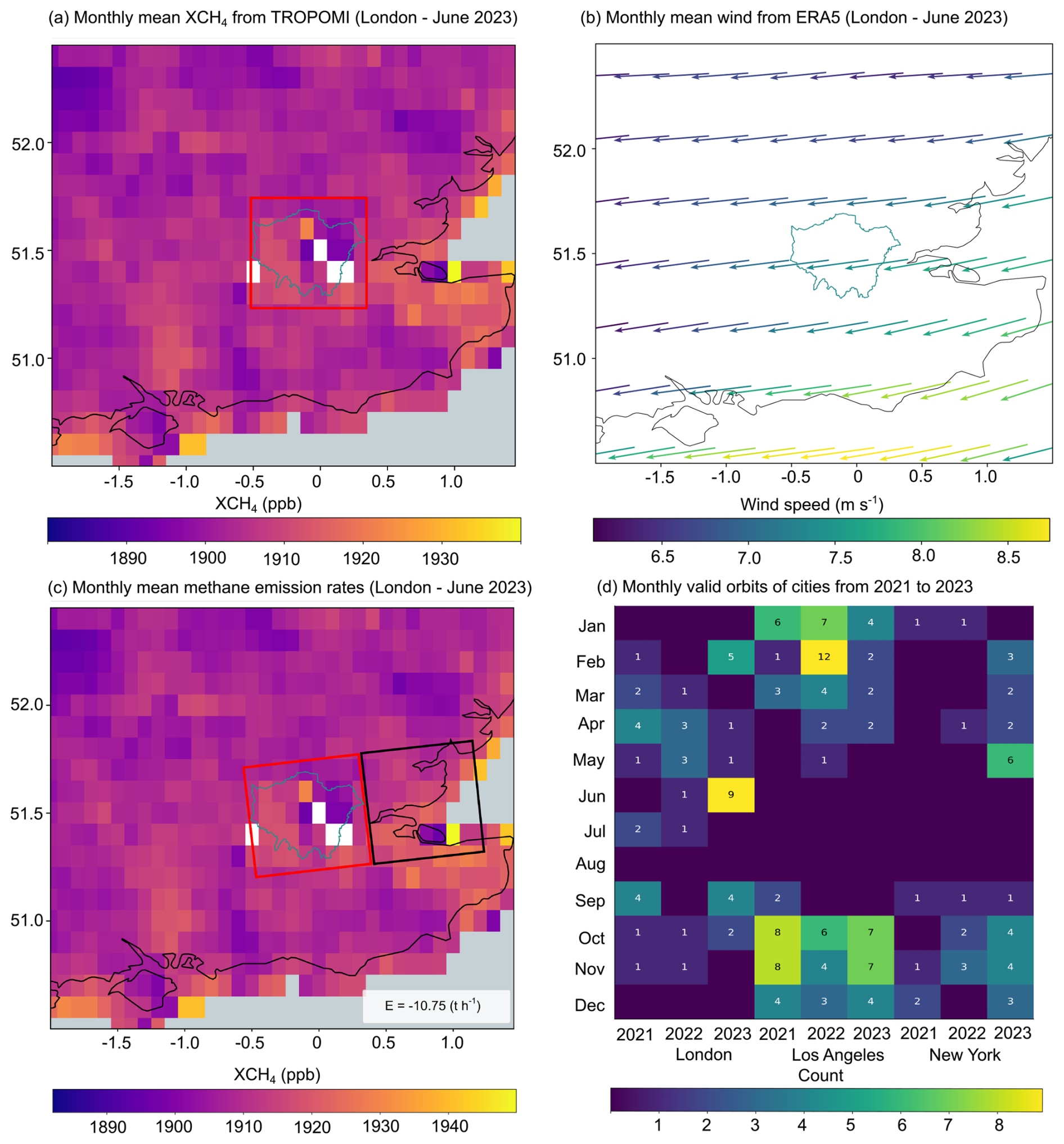
Figure 3 Illustration of the upwind background determination based on the improved source pixel method used in this study. (a) Mean XCH₄ retrievals derived from the TROPOMI instrument for London in June 2023. (b) Monthly mean wind vectors derived from hourly resolved ERA5 reanalysis data set for London in June 2023. (c) Location of the immediately adjacent upwind background region defined according to the wind direction shown in panel (b). (d) Monthly number of valid satellite overpasses for the three cities during 2021–2023 that passed strict quality control and were used in the final emission estimates.

An illustrative example of the improved source pixel method used in this study is shown in Fig. 3 for London, demonstrating how the retrieved methane enhancement over the source region (ΔXCH₄) is defined and oriented to the ERA5 wind direction and the corresponding location of the up-wind background region. To compute the PBL wind speed and direction, ERA5 hourly wind products are gridded onto the same spatial grid as TROPOMI data (Fig. 3b). After calculating the pressure-weighted average wind vector in the PBL over source region, the location of the up-wind background is obtained, as shown in Fig. 3c. Using this method, the valid orbits that pass through the satellite configuration filters, coverage threshold and uncertainty threshold, vary significantly across years and in different months. In Fig. 3d, the lowest observation is in New York city in 2021, with only 5 valid orbits that overpass the urban domain. Coverage increases to 8 and 25 overpass in 2022 and 2023, but the month-to-month variation is notable with most of the orbits observed in spring and winter seasons. Los Angeles has the largest coverage, nearly 100 total single orbits are usable in the method from 2021 to 2023. The number of annual valid satellite overpass over London urban area are between 10 and 25 orbits, and mostly are observed in spring, summer and winter seasons (as might be expected due to autumn storms and cloud). Clearly, such seasonality and inter-year variability in the number of valid scenes can be expected to lead to bias. This would be expected to be a limitation inherent to any application of the source pixel method using TROPOMI, even without the additional filtering we have applied here to reduce potential bias associated with cloudy scenes. We highlight this problem here as an honest appraisal of the challenges and limitations of using satellite data for urban emissions quantification. Put simply, biases implicit to sampling may remain, despite any attempt to minimize their presence. Therefore, when comparing annualized emissions by the improved method in this study (or any other) with inventories, it is important to be cognizant of how such biases may manifest; for example in the context of which periods of a given year may be poorly sampled compared to others and whether this may expected to manifest as a low or high bias overall versus perfect year-round sampling.

2.4 Emission uncertainty quantification

To estimate the uncertainty of urban emission rates, we assess the influence of uncertainties in ΔXCH₄ and U, which can be derived statistically from TROPOMI and ERA5 data products. This procedure captures the potential sensitivity of systematic errors in the retrieved column mixing ratio over source pixels and uncertainty in the background estimate used to define methane enhancements. Also, the simulation of the constant wind within source region can result in large uncertainty because of changes in wind direction over the course of a typical day (Varon et al., 2018).

When assessing the ΔXCH₄ uncertainty, the satellite retrieval measurements of atmospheric albedo and aerosol in SWIR band are involved. They may cause an overestimate or underestimate of the average column dry air mixing ratio relative to its real abundance through lengthening or shortening the light path (Jacob et al., 2016). To calculate the error of methane enhancement results from the albedo and aerosol difference in the source region and background region, we use a linear fitting method to simulate the relationship between the column methane XCH₄ and the factors of albedo and aerosol within the source or background regions. The uncertainty of wind speed is estimated from the standard deviation of wind speed over the source region in a period of four consecutive hours around the TROPOMI local overpass time. Then, a representative statistical confidence error of emission rates σ_E for a single scene is computed as the sum in quadrature of 1σ of methane enhancement and wind speed.

$$\begin{array}{}\text{(3)}& y=ax+b\end{array}$$

$$\begin{array}{}\text{(4)}& {\displaystyle }{\mathit{\sigma }}_{\mathrm{\Delta }{\mathrm{XCH}}_{\mathrm{4}}}=\sqrt{\begin{array}{c}{\left[a_{\mathrm{alb}}(x_{\mathrm{SR},\mathrm{alb}}-x_{\mathrm{BR},\mathrm{alb}})\right]}^{\mathrm{2}}+\\ {\left[a_{\mathrm{aer}}(x_{\mathrm{SR},\mathrm{aer}}-x_{\mathrm{BR},\mathrm{aer}})\right]}^{\mathrm{2}}\end{array}}\text{(5)}& {\displaystyle }{\mathit{\sigma }}_E=E\cdot \sqrt{{\left({\displaystyle \frac{{\mathit{\sigma }}_{\mathrm{\Delta }{\mathrm{XCH}}_{\mathrm{4}}}}{\mathrm{\Delta }{\mathrm{XCH}}_{\mathrm{4}}}}\right)}^{\mathrm{2}}+{\left({\displaystyle \frac{{\mathit{\sigma }}_U}{U}}\right)}^{\mathrm{2}}}\end{array}$$

Here, a_alb and a_aer denote the slopes of the linear regression (Eq. 3) obtained by regressing XCH₄ against surface albedo and aerosol optical thickness, respectively, within the study domain. x_SR and x_BR refer to the mean value of albedo or aerosol in the source region and background region.

For urban areas that have multiple valid overpasses (i.e. days), the emission rates and uncertainties need to be averaged to generate total urban estimates at the desired timescale (e.g. monthly or yearly). To ensure the quality of results, we only include orbits with uncertainties of less than 100 %. Most previous studies using the source pixel method have analyzed aggregated emissions at monthly or yearly timescales from orbit-level estimates by assigning equal weight to each overpass, regardless of whether the overpass has limited or full valid data coverage over the source region. In this study, we use spatial coverage (in %) of valid observations in the source region to weight each overpass during averaging, in an effort to reduce spatial bias arising from potential heterogeneity in methane mixing ratios. Note that potential surface emission transfer among different pixels is not considered. Finally, the uncertainty in the temporally-averaged estimates is calculated as the root mean square error (RMSE), in Eq. (6).

$$\begin{array}{}\text{(6)}& \mathrm{RMSE}\left(\mathit{\%}\right)={\displaystyle \frac{\sqrt{\frac{\mathrm{1}}{N}{\sum }_{i=\mathrm{1}}^N({\mathit{\sigma }}_{E_i}{)}^{\mathrm{2}}}}{\frac{\mathrm{1}}{N}{\sum }_{i=\mathrm{1}}^N{E}_i}}\times \mathrm{100}\end{array}$$

Where ${\mathit{\sigma }}_{E_i}$ refers to the uncertainty of emission rate for orbit i (Eq. 5), and E_i denotes the calculated emission rate of orbit i, N is the valid overpass of TROPOMI for a given urban domain that restricted by cloud, water, and oceans, etc.

3 Results

3.1 Urban emissions in London

The urban domain used to implement the improved source pixel method of this work is defined over London, a source region that has been the topic of numerous methane emission studies (Helfter et al., 2016; Pitt et al., 2019). The results for 2021–2023 are summarized in Fig. 4. Figure 4a presents the spatial distribution of mean XCH₄ levels over London urban area for the study period. The urban enhancement relative to the surrounding background is generally modest, with no persistently strong hotspot visible within the defined source region. The relatively weak spatial contrast implies that the calculated ΔXCH₄ is sensitive to background variability (As shown in Fig. A3). In particular, when the upwind sector (e.g. background XCH₄) contains elevated methane from other nearby source regions, the derived ΔXCH₄ over the study area can be substantially reduced and may occasionally become negative (see Sect. 2.3). This result is consistent with previous aircraft-based and dispersion modeling analyses over London (Pitt et al., 2019), which also reported relatively small urban-scale enhancements. The corresponding monthly time series of ΔXCH₄ of London urban area is shown in Fig. 4c. The annual mean enhancement increased from 1.47±0.76 ppb in 2021 to 1.98±1.38 ppb in 2022, before slightly declining to 1.70±0.83 ppb in 2023. A clear seasonal cycle is observed in the monthly average ΔXCH₄, with larger enhancements during winter months. This seasonality likely reflects a combination of increased emissions and more stable atmospheric conditions. It should also be noted that data coverage is uneven throughout the year due to cloud contamination, which reduces the number of valid TROPOMI overpasses in certain months. Figure 4b presents estimated methane emission rates for London from 2021 to 2023, derived using the method outlined in Sect.  2.3. The 3-year mean emission rate is 7.78±4.84 t h⁻¹, where the long-term uncertainty is estimated from multiple satellite overpasses following Eq. (6). The annual mean emissions are 5.99±3.25 t h⁻¹ (2021), 11.90±8.56 t h⁻¹ (2022), and 7.25±4.64 t h⁻¹ (2023). The relatively low estimate in 2021 is primarily driven by an anomalously low value in October, when background XCH₄ exceeded concentrations within the urban domain, resulting in near-zero or negative ΔXCH₄. If this month is excluded as a statistical outlier, the 2021 annual emission increases to 10.11±6.28 t h⁻¹, highlighting the sensitivity of the method to background characterization under weak enhancement conditions. The mean wind speed over the urban domain during 2021 to 2023 is 5.15±0.55 m s⁻¹, with pronounced seasonal variability (Fig. 4d). Comparison of Fig. 4b–d indicates that temporal variations in emission estimates are primarily controlled by variability in ΔXCH₄ rather than wind speed. Uncertainty propagation analysis attributes approximately 80 % of the total emission uncertainty to variability in the methane enhancement, whereas wind-related uncertainty only accounts for about 20 %. This result underscores that, for weakly enhanced urban regions (such as London), accurate background determination and robust enhancement retrievals are the dominant factors governing emission estimate reliability.

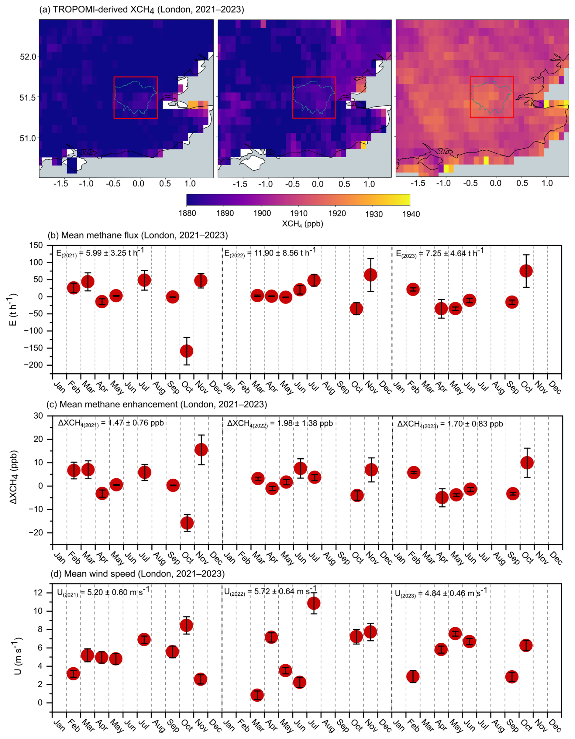
Figure 4 Results for the London urban area during 2021–2023. (a) Spatial distribution of TROPOMI-derived XCH₄, with the defined source box outlined in red based on the blue administrative boundary. (b) Monthly mean methane emission rates derived using the improved source pixel method. (c) Mean methane enhancement. (d) Mean wind speed.

The bottom-up methane emissions for the London urban area, as reported by the EDGAR inventory, are shown in Fig. A1a. To ensure direct comparability with top-down estimates in this work, the gridded EDGAR emissions were extracted and summed over the same source box defined in Sect. 2.1.4. In this way, both bottom-up and satellite-based emissions refer to an identical spatial domain. The EDGAR-derived emissions are significantly lower than the satellite-based emission rates estimated using the improved source pixel method. Over the same spatial domain and time period, the top-town emission estimates in this work are approximately 2.1 times higher than the EDGAR inventory values. According to EDGAR, the dominant methane source in London during 2021–2023 is waste management, contributing on average approximately 63 % of the total emissions (Fig. A4a). Fossil fuel-related emissions (e.g. leakage from natural gas transmission and distribution systems) represent the second largest source, accounting for about 32 %, followed by agriculture activities (nearly 5 % of total emission). Other sectors (e.g., wetlands and other anthropogenic sources) contribute comparatively smaller fractions.

3.2 Urban emissions in Los Angeles

Methane emissions over the Los Angeles urban area for the period 2021–2023 were estimated using the same improved source pixel method. The results are summarized in Fig. 5, along with the mask that delineates the source region. The spatial distribution of TROPOMI-derived XCH₄ in Los Angeles city (Fig. 5a) reveals a pronounced methane hotspot over the defined urban domain, with clearly elevated concentrations relative to the surrounding background. In contrast to London, the methane enhancement over Los Angeles is spatially coherent and persistent, indicating a strong urban emission signal detectable from space. The 3-year average emission estimate from 2021 to 2023 is 47.19 t h⁻¹, with a 1σ uncertainty range spanning from 13.51 to 80.87 t h⁻¹. As shown in Fig.  5b, the annual mean methane emissions increase from 26.21±23.03 t h⁻¹ in 2021 to 50.18±36.55 t h⁻¹ in 2022 and further to 62.77±35.95 t h⁻¹ in 2023, indicating a substantial interannual growth over the study period. Although this apparent increase is inconsistent with the decreasing trends reported in previous studies (Zeng et al., 2023; Schafer et al., 2025; Yadav et al., 2023), the large uncertainties in the annual estimates and their substantial overlap indicate that a decreasing trend similar to those reported previously cannot be ruled out. A clear seasonal pattern is apparent, with higher emission estimates generally occurring during winter and early spring. Notably, little to no valid emission estimates are available during the summer months, particularly in 2021 and 2023, likely due to persistent marine boundary layer clouds and coastal meteorological conditions that substantially reduce the number of usable satellite overpasses (e.g. insufficient valid pixels are available within either the source region or the upwind background region to satisfy the data quality thresholds defined in Sect. 2.1.1 and 2.3). Figure 5c and d show that the average methane enhancement ΔXCH₄ over the study period is 10.66±5.87 ppb, while the mean wind speed is 2.96±1.10 m s⁻¹. Although the seasonal variation of emission rate broadly follows that of ΔXCH₄, uncertainty analysis indicates that more than half of the total emission uncertainty is attributable to wind variability. This reflects the sensitivity of the emission rates calculation to wind speed during the satellite overpass window (19:00, 20:00, 21:00, 22:00 UTC), when coastal circulations and ocean–land breeze dynamics can induce substantial short-term wind fluctuations over the Los Angeles basin.

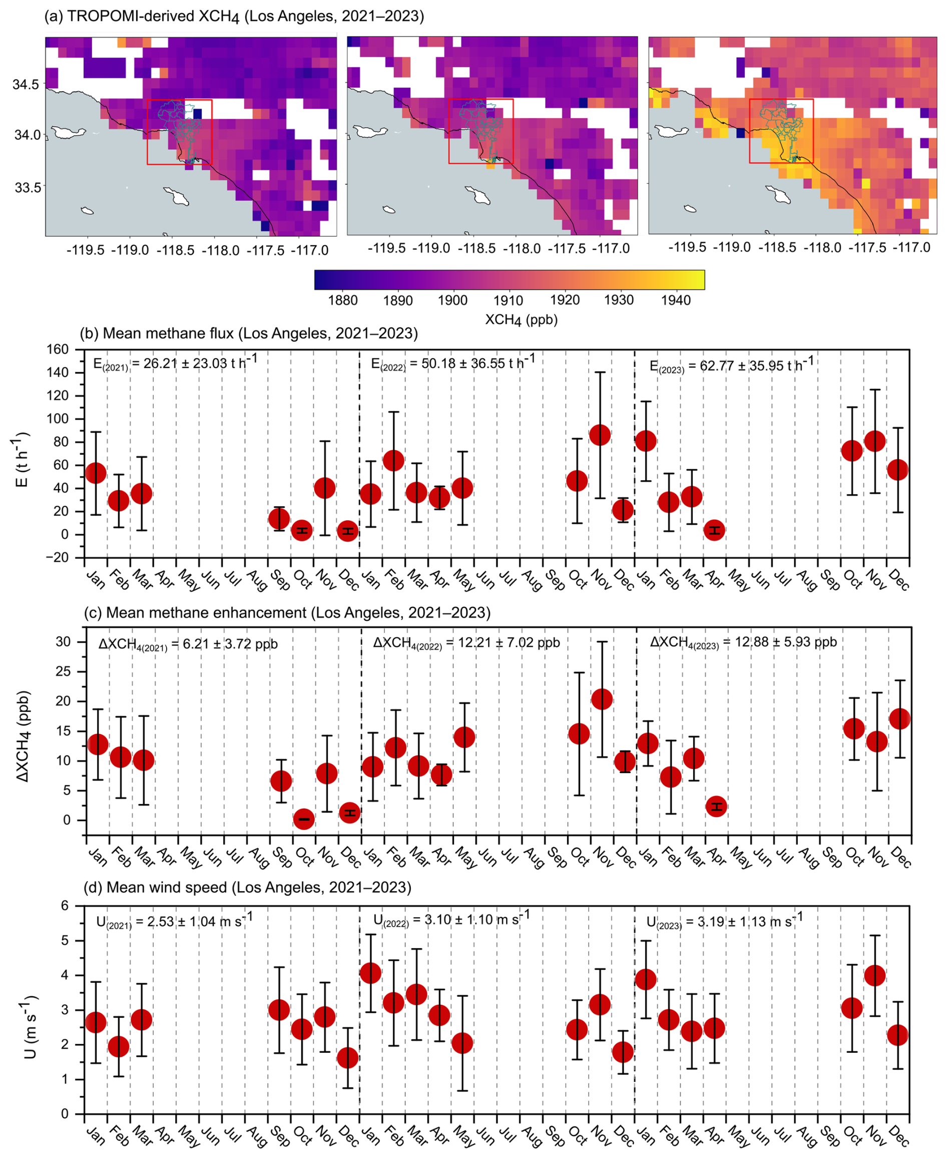
Figure 5 Results for the Los Angeles urban area during 2021–2023. (a) Spatial distribution of TROPOMI-derived XCH₄, with the defined source region outlined in red based on the blue administrative boundary. (b) Monthly mean methane emission rate derived using the improved source pixel method. (c) Mean methane enhancement. (d) Mean wind speed.

The spatial distribution of methane emissions from the EDGAR inventory for 2021–2023 is shown in Fig. A1b. When aggregated over the identical source domain used in the this work, the mean EDGAR emission for Los Angeles urban area is 20.07 t h⁻¹, which is notably lower than the satellite-derived estimate of 47.19±33.68 t h⁻¹. Sectoral attribution (see Fig. A4b) indicates that Los Angeles is dominated by waste-related emissions, primarily from landfills, which account for more than 90 % of the total methane emissions in each study year. Fossil fuel-related sources represent a much smaller contribution, approximately 9 % of the total.

3.3 Urban emissions in New York

New York serves as the third case study for evaluating the improved source pixel method. The corresponding results for 2021–2023 are summarized in Fig. 6. The TROPOMI-derived XCH₄ fields (Fig. 6a) exhibit a discernible enhancement over the defined urban domain, particularly in 2022 and 2023, indicating a persistent methane signal relative to the surrounding background. However, the geographic setting of New York – located at the confluence of major waterways and influenced by frequent cloud cover – limits the number of valid satellite retrievals in certain months, especially during the 2021 and 2022. The temporal evolution of the derived methane emission rate is shown in Fig. 6b. The three-year mean emission is 42.94 t h⁻¹ with a standard deviation of 24.69 t h⁻¹. Among the individual year, 2023 exhibits the highest annual mean emission rate (44.77±25.03 t h⁻¹), whereas 2022 shows the lowest (30.85±21.50 t h⁻¹). Monthly variability reveals a recurring seasonal structure, with relatively elevated emissions during early autumn, particularly in September. In contrast to the other two years, 2023 provides more continuous data coverage, with valid emission estimates available for most non-summer months. However, June–August remain largely data-limited, and intermittent gaps are still evident due to cloud contamination and quality-control filtering of satellite retrievals. Figure 6c and d indicate a mean methane enhancement of 9.15±5.72 ppb and an average wind speed of 5.43±0.91 m s⁻¹ over the study period. Although seasonal variations in emission rates are primarily driven by changes in methane enhancement within the source region relative to the background, wind variability plays a non-negligible role in modulating the magnitude of the calculated emissions. The relatively strong and seasonally variable winds over New York introduce additional variability during the satellite overpass window. Uncertainty analysis shows that methane enhancement accounts for approximately 60 % of the total emission uncertainty, while wind contributes the remaining 40 %, indicating a more balanced uncertainty structure compared to Los Angeles.

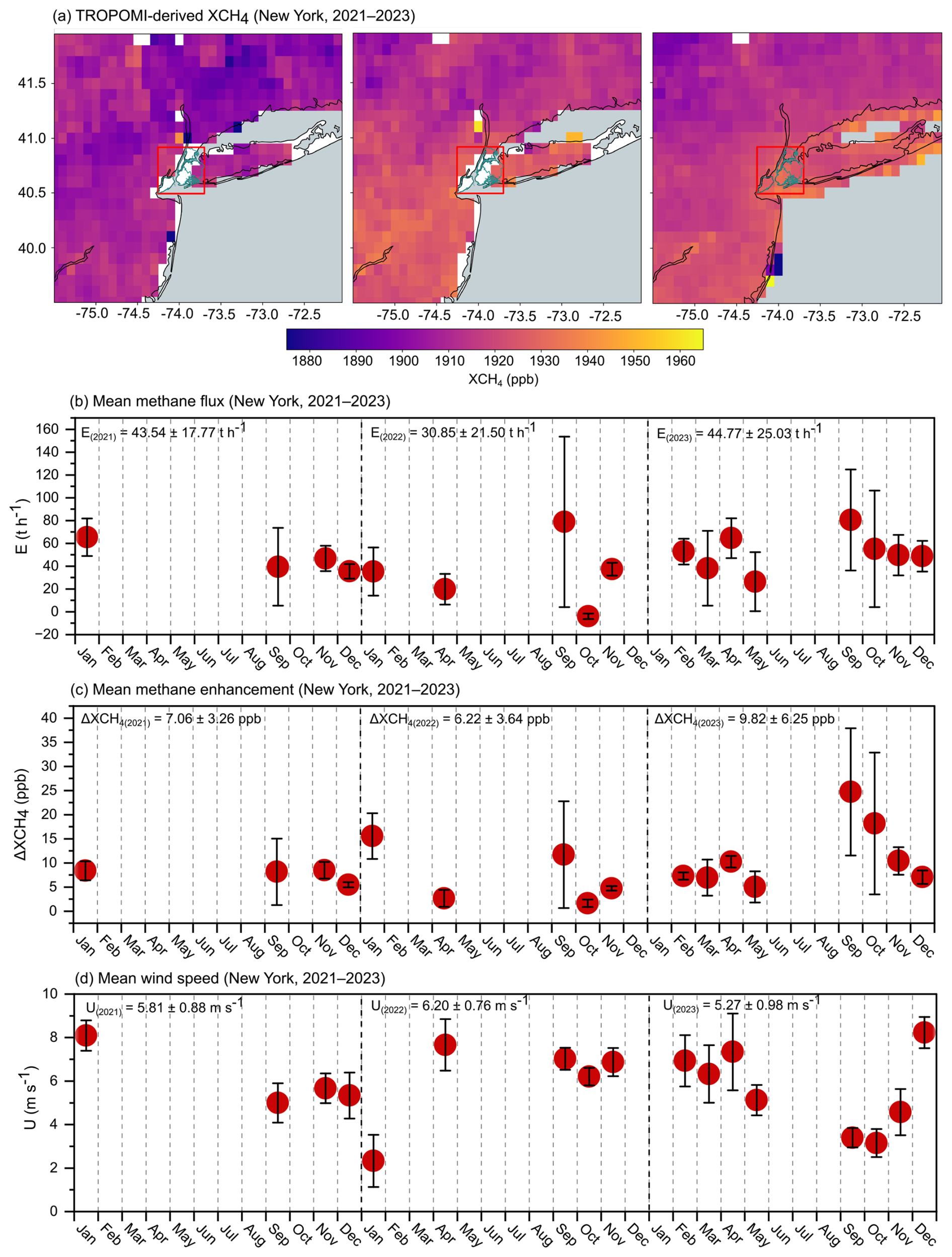
Figure 6 Results for the New York urban area during 2021–2023. (a) Spatial distribution of TROPOMI-derived XCH₄, with the defined region outlined in red based on the administrative boundary (blue). (b) Monthly mean methane emission rate derived using the improved source pixel method. (c) Mean methane enhancement. (d) Mean wind speed.

The spatial distribution of EDGAR gridded methane emissions for New York city is shown in Fig. A1c. Emissions within the urban area are relatively weak and spatially diffuse, with only a few grid cells exhibiting moderate emission values. When aggregated over the identical source box used in this work (red box), the annual mean methane emission for the EDGAR inventory is 4.38 t h⁻¹ for 2021–2023. This value is substantially lower than the satellite-derived estimate and corresponds to approximately 11 % of the emission magnitude inferred from the improved source pixel method. Sectoral attribution indicates that emissions are dominated by waste-related sources (e.g. solid waste and waste water), contributing about 53 % of the total, followed closely by fossil fuel-related activities at approximately 45 %. Other sectors represent only a minor fraction of the inventory-based emissions (Fig. A4c).

3.4 Comparison with inventories and previous studies

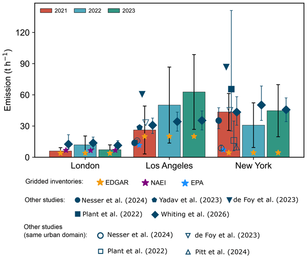
Figure 7 presents a comparison between our satellite-derived emission estimates based on improved source pixel method, three widely used gridded bottom-up inventories, and six recently published top-down studies. Overall, our estimates consistently exceed the gridded inventory values across all three cities, ranging from 1.3 to 10.2 times the publicly available EDGAR inventory. For London, comparison between emission estimates derived from our study and the NAEI inventory (Tsagatakis et al., 2024) indicates that bottom-up estimates generally underestimate urban methane emissions, with the exception of 2021, and the discrepancy reaches up to 45 % in 2022. For the U.S. cities, the EPA inventory (Maasakkers et al., 2023) similarly reports lower emissions than our satellite-based results, with underestimations of approximately 56 % for Los Angeles and 84 % for New York.

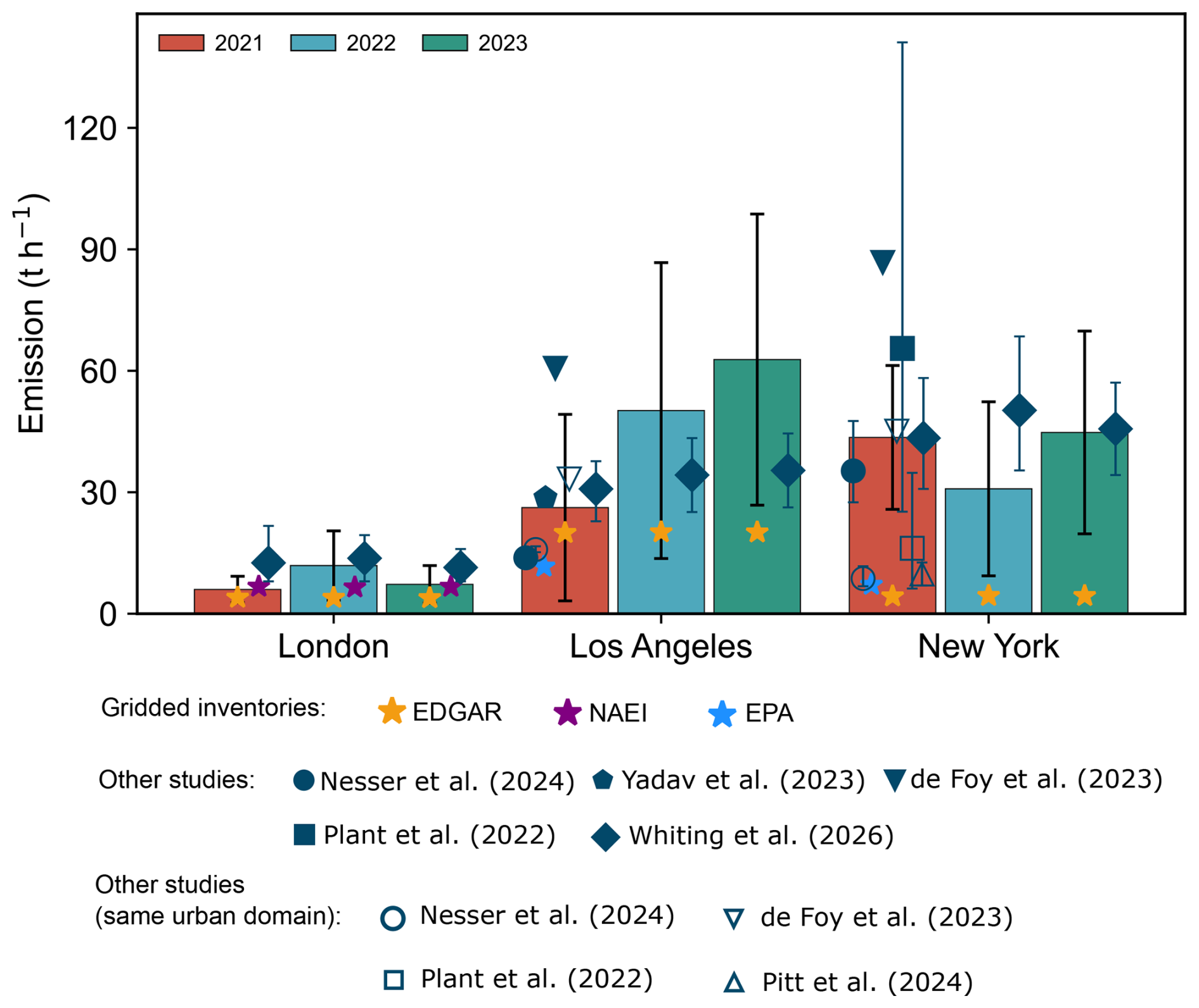
Figure 7 Comparison of annual methane emissions for the three case-study cities (2021–2023), including satellite-derived estimates based on improved source pixel method from this work, gridded bottom-up inventories, and previously published top-down studies.

The magnitude of city-scale methane emission estimates can vary substantially depending on how the urban domain is delineated, particularly when large point sources, such as landfills, are located along the urban fringe. These studies adopt different definitions of urban area and generally include contributions from nearly all source sectors. For example, Plant et al. (2022) and Nesser et al. (2024) quantify urban emissions based on the U.S. Census Bureau's Topologically Integrated Geographic Encoding and Referencing system (TIGER)/Line urban area definitions to standardize the spatial extent across the contiguous United States (CONUS) (U.S. Census Bureau, 2017). Most studies use aircraft measurements, tower observations or satellite retrievals combined with atmospheric chemical transport models to infer methane emissions (Nesser et al., 2024; Pitt et al., 2024; Yadav et al., 2023), while others use characteristic urban $\mathrm{\Delta }{\mathrm{CH}}_{\mathrm{4}}/\mathrm{\Delta }\mathrm{CO}$ enhancement ratios integrated with existing inventories to estimate methane emission rates (Plant et al., 2022; Whiting et al., 2026). de Foy et al. (2023) applied a two-dimensional Gaussian model to estimate the local emissions required to reproduce the observed satellite retrievals. Our emission estimates can be directly compared on a like-for-like basis only with those of Pitt et al. (2024), who developed a new high-resolution (0.02°×0.02°) methane emission inventory for New York for 2019 based on an analytical inversion of aircraft measurements. Even when using the same gridded urban domain, a large discrepancy remains, which may be largely attributable to differences in the reporting period. Direct comparisons between our results and urban emission estimates from other studies remain challenging because of differences in urban domain definitions and reporting periods, as discussed in previous studies (Nesser et al., 2024; Wang et al., 2026). Overall, the estimates reported in these studies are broadly consistent with ours, with most falling within our uncertainty bounds, except for those of de Foy et al. (2023), which represent relatively high urban-scale emission estimates.

To ensure spatial consistency in the comparison, we converted the reported emissions from previous studies into emission intensities (emission rate per unit area) and subsequently rescaled them to our defined urban domain. Yadav et al. (2023) reported a posterior estimate of 28.65±0.55 t h⁻¹ based on sustained station observations for Los Angeles, which is very close to our estimate of 26.21±23.03 t h⁻¹. A study using TROPOMI observations to estimate methane emissions over U.S. urban areas reported substantially higher values of 60.62 t h⁻¹ for Los Angeles and 86.76 t h⁻¹ for New York (de Foy et al., 2023). However, after scaling their estimates to the same urban domain used in this work, these values decrease to 33.27 and 45.09 t h⁻¹, respectively, which align well with our results. Plant et al. (2022) and Nesser et al. (2024) adopted the same U.S. Census urban area definition but applied different emission quantification methods. They found different emission estimates for New York city, although the reported ranges largely overlap with the uncertainty bounds of our derived emissions. After scaling to the same urban domain, our estimated emission range remains consistent with the uncertainty reported by Plant et al. (2022), while remaining higher than the estimate from Nesser et al. (2024). For Los Angeles, although our study employs a different definition of urban boundary and a different emission quantification method, our estimates remain consistent with those of Nesser et al. (2024) under both scaled and non-scaled conditions. We need to acknowledge the relatively large uncertainty involved in this rescaling, especially considering the heterogeneous attribution of urban emission sources such as landfills and gas infrastructure. Given the relatively strict urban domain defined in our study based on administrative boundaries, as well as the use of different emission quantification methods, our emission estimates are likely to approach those reported by de Foy et al. (2023) if more suburban emission sources are included.

4 Conclusions

This study presented a framework for monitoring, identifying, and quantifying urban methane emissions using TROPOMI retrievals in combination with an improved source pixel method. The methodological advancement lies in the incorporation of hourly resolved PBL-pressure weighted wind fields and an explicitly defined upwind background concentration. These refinements enhance the conceptual accuracy of the approach relative to the conventional source pixel method, which does not explicitly account for upwind background direction or the vertical structure of wind within PBL. The principal advantage of this method is that emissions can be inferred directly from satellite-observed methane enhancements over the elevated source region relative to their surrounding areas, along with a representative advective mean wind vector. We applied the improved method to TROPOMI observations over three major cities (London, Los Angeles, and New York) during 2021–2023 to quantify orbit-level methane emissions and associated emission uncertainties. The satellite-derived estimates were further compared with widely used gridded bottom-up inventories and recently published top-down studies. Overall, our estimates consistently exceed the gridded inventory values across all three cities, although great inter-annual and inter-city variability is observed. When compared with previous top-down studies, our results are generally consistent with the reported emission estimates, with most estimates falling within our uncertainty bounds. The inconsistencies between different top-down emission estimates and bottom-up inventories have been well documented in previous studies, and they do remain despite this study. But we hope we can offer an improved method with greater possibility for repeatability going forward. Discrepancies can be partially attributed to the thermodynamic variability (i.e. wind fields) within the planetary boundary layer and the methods used to define background concentrations. In addition, inconsistencies among previous top-down studies are largely driven by differences in the definition of what constitutes the urban area of interest (i.e. city boundary) and the reporting periods (i.e. timescales), which makes direct comparison between studies challenging. By integrating pressure-weighted winds under the planetary boundary layer with an upwind background concentration approach, the method we describe could help bridge methodological differences in flux quantification by providing a more repeatable methodology and approach to urban boundary definitions.

Emission uncertainties in this study are typically on the order of tens of percent, comparable to those found by Buchwitz et al. (2017), who estimated relative uncertainties of about 50 % for large emissions sources (i.e. several Mt CH₄ yr⁻¹). A significant reason for this is that methane enhancement estimates are sensitive to background variability; however, when the signal over the urban area is proportionately larger than the surrounding background and background is less variable, the resulting emission uncertainty is significantly reduced. To reduce systematic uncertainties arising principally from cloud cover, heterogeneous albedo of coast pixels, and aerosol scattering, we retained only high-quality XCH₄ retrievals under cloud-free conditions and applied strict filtering criteria (Sect. 2.1) to exclude pixels with poor spectral fits and other retrieval artifacts. Additional filtering thresholds were introduced in the final emission estimates to minimize the influence of limited sampling and potential outliers that passed earlier constraints. These stringent filtering criteria inevitably resulted in the exclusion of a substantial fraction of satellite overpasses, representing a key limitation of the method used in this work. The reduced data coverage may introduce biases in the inferred seasonal and inter-annual variability. However, we argue that this trade-off is necessary to preserve statistical reliability and avoid systematic overestimation or underestimation of emissions. These considerations highlight the importance of understanding how such biases may manifest when comparing annualized emissions derived from the source pixel method using satellite retrievals. Our results provide evidence that satellite observations can serve as a promising technology for ongoing city-scale emission detection, reconciliation, and reporting through long-term global monitoring, which helps build methane emission characteristics and track whether emission targets are being met.

Appendix A

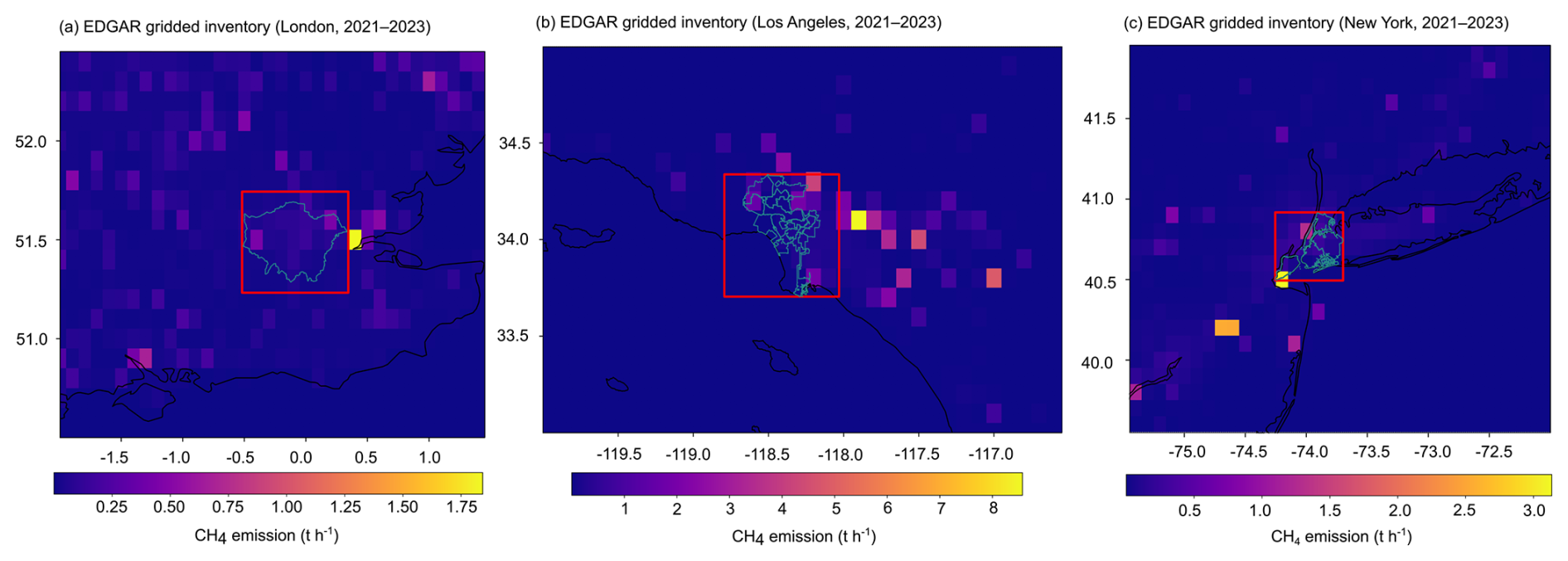
Figure A1 Annual average of emission inventories from EDGAR datasets for London (a), Los Angeles (b) and New York (c) from 2021 to 2023.

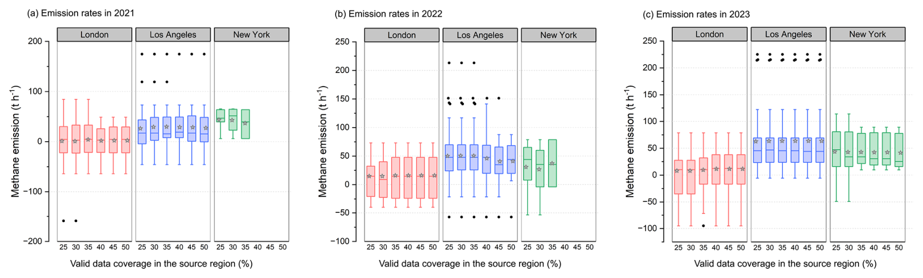
Figure A2 Sensitivity of emission rates in three case study cities to populated valid data coverage in the source region after filtering, shown for (a) 2021, (b) 2022, and (c) 2023.

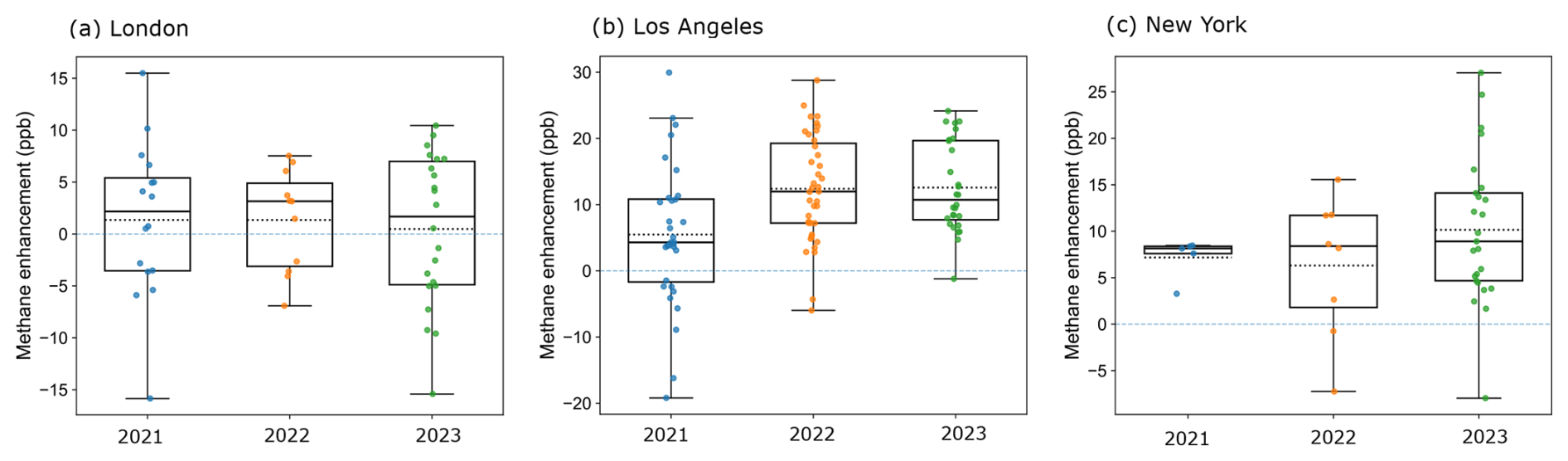
Figure A3 Boxplot of methane enhancement for each overpass in London (a), Los Angeles (b) and New York (c) from 2021 to 2023.

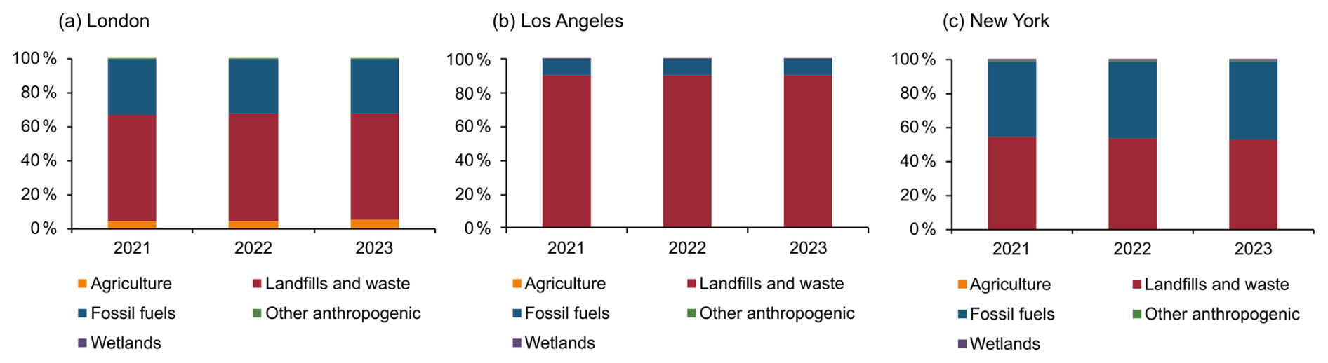
Figure A4 Fractions of four major aggregated emission sectors from EDGAR inventory and natural wetland emissions from WetCHARTs in (a) London, (b) Los Angeles, and (c) New York.