Evaluation of a moist-adiabat cloud-top height retrieval for parallax correction of deep convective clouds across Meteosat generations

Accurate estimation of deep convective cloud (DCC) top height is essential for reliable parallax correction of geostationary satellite imagery and for constructing homogeneous long-term climatologies from multi-generation meteorological satellite records (e.g. Meteosat MVIRI, SEVIRI, and FCI). This study validates the cloud-top height (CTH) retrieval method of Šoljan et al. (2024), which estimates cloud-top pressure in deep moist convection from satellite-derived 11 µm brightness temperature using a fast polynomial approximation of the moist adiabat. The primary objective is to assess whether this method enables parallax correction consistent with operational products across more than 40 years of Meteosat data, including early missions lacking multispectral capability.

Validation was conducted in two configurations reflecting polar-orbiting and geostationary viewing geometries. First, approximately 1.7 million DCC collocations from 2007 were used to compare CTH estimates with MODIS retrievals and lidar–radar profiles from CloudSat and CALIPSO. Second, a SEVIRI time series from 2004 to 2024 was evaluated against the operational CLAAS-3 CTH product. Overall, the method underestimated CTH by 2.7 km (18 %) relative to lidar–radar data and by 1.1 km (10 %) relative to CLAAS, with mean absolute errors of 1.5–2.8 km and correlations up to 0.9. Following a simple regression-based bias adjustment, normalized errors decreased to below 7 % and absolute errors fell below 1.2 km.

The method was subsequently applied to SEVIRI observations to assess its suitability for parallax correction over the European domain. Despite a ∼10 % underestimation of CTH, the impact on parallax correction was minimal: 84 % of pixel geolocations coincided with those derived from CLAAS-based corrections, increasing to 97 % when CLAAS retrieval uncertainty was accounted for. Differences in DCC frequency remained below 7 % on a monthly scale and below 5 % seasonally. These results demonstrate that the method provides operationally sufficient accuracy for parallax correction of DCCs and supports the development of a homogeneous DCC climatology across all generations of Meteosat satellites and, potentially, other geostationary platforms.

1 Introduction

Any off-nadir observation of the Earth acquired from orbit is affected by parallax. Elevated objects viewed at an angle appear displaced farther from the sub-satellite point than their true location. The magnitude of this parallax shift increases with both the viewing angle and the elevation of the observed target. While this effect can be advantageous for stereo mapping (Abrams et al., 2010; Moroney et al., 2002), it poses a significant challenge for the accurate geolocation of elevated atmospheric features. High-level clouds are among the most strongly affected, including deep convective clouds (DCCs), whose tops can approach the tropopause at altitudes of approximately 10–15 km above sea level.

DCCs are associated with severe weather phenomena such as heavy precipitation, hail, lightning, tornadoes, and damaging winds. A single severe deep convective storm can cause average insured losses of about USD 100 million (Changnon, 2011), in addition to causing significant damage to property and risk to human life (Pilorz et al., 2023). DCC-related weather also poses a substantial hazard to aviation, affecting both flight safety (Gultepe et al., 2019) and economic efficiency (Sauer et al., 2019). At the same time, DCCs play an important role in the climate system, contributing significantly to large-scale mass transport, the hydrological cycle, and the global energy balance (Chae et al., 2011; Hartmann et al., 2001).

Accurate geolocation of DCCs is therefore essential for both meteorological and climatological applications. Because they evolve rapidly, their monitoring over large spatial domains relies primarily on observations from geostationary satellites. However, the geostationary viewing geometry introduces substantial parallax distortions in DCC imagery, particularly at large viewing angles away from nadir. This effect is especially pronounced over Europe, which has been continuously observed by Meteosat satellites of the first (de Waard et al., 2025), second (Schmetz et al., 2002), and third (Holmlund et al., 2021) generations from a nominal geostationary position at 0° E.

DCCs are relatively infrequent, which means that even minor errors in their geolocation can lead to substantial relative uncertainties in estimating their frequency of occurrence. However, the parallax effect itself is well described mathematically (Bieliński, 2020; Vicente et al., 2002), and satellite observations can be corrected for parallax provided that both the satellite viewing geometry and the altitude of the observed target – typically represented by cloud-top height (CTH) – are known. The satellite position can be readily obtained from orbital data, whereas reliable CTH retrieval remains a major challenge.

The most accurate CTH estimates are obtained from spaceborne lidars, which emit optical pulses in the ultraviolet, visible, or near-infrared and profile the atmosphere in nadir-viewing geometry, achieving accuracies on the order of tens of metres. However, their very narrow fields of view (swath widths below 1 km) result in sparse spatial and temporal sampling (Kotarba, 2022). This limitation can be partially addressed by complementary radar observations, which are sensitive to optically thick clouds where the lidar signal is attenuated, and by wide-swath imaging radiometry.

Wide-swath CTH retrievals are obtained either photogrammetrically – by exploiting parallax from two or more vantage points, whether through sequential along-track imaging (Anzalone et al., 2019; Lancaster et al., 2003), multi-angle viewing (Diner et al., 1998; Muller et al., 2007), or stereo pairs from independent satellites (Hasler, 1981; Seiz et al., 2007) – or radiatively, through differential absorption in the CO₂ band at 15 µm (CO₂ slicing; Menzel et al., 2008), the O₂ A-band (0.76 µm), or the H₂O band (6.7 µm).

While these approaches treat CTH as a single retrieved quantity, optimal estimation methods go further by simultaneously retrieving multiple cloud properties. The most probable atmospheric state is found by minimising the difference between observed and modelled radiances, subject to a priori constraints (Heidinger and Pavolonis, 2009; Rodgers, 1976). More recently, machine-learning approaches trained on collocated lidar and radar reference data have demonstrated considerable promise for CTH retrieval (Håkansson et al., 2018; Min et al., 2020; Tan et al., 2022; White et al., 2022).

All of the methods described above require either multispectral observations including absorption bands, multi-angle viewing geometry, or high-quality reference data for machine-learning model training. However, these requirements cannot be met when CTH estimation relies on brightness temperature (BT) from a single infrared channel, as is the case for early geostationary satellites such as Meteosat First Generation. Under such constraints, a simplified approach must be adopted.

The standard simplification assumes that the cloud radiates as a blackbody, so that its cloud-top temperature can be represented by the BT in the infrared window channel (11 µm). This provides an acceptable approximation for optically thick clouds, including DCCs, although it is not strictly valid for thin, semi-transparent, or multi-layered clouds. Assuming further that the cloud top is in thermal equilibrium with the surrounding atmosphere, CTH is determined as the altitude at which the atmospheric temperature profile equals the observed BT (Koffler et al., 1973). The required temperature profile may be obtained from radiosondes, numerical weather prediction (NWP) models, reanalysis, or climatology.

For DCCs specifically, however, the full vertical temperature profile may not be necessary. Since DCCs develop along the moist adiabat, CTH can instead be inferred by matching the satellite-derived BT with the temperature of a rising air parcel computed along the pseudoadiabat. When the moist adiabat is approximated using polynomials, rather than computed iteratively (Moisseeva and Stull, 2017; Šoljan et al., 2024), the approach becomes computationally efficient and well suited to processing large volumes of remote sensing data, enabling the generation of parallax-corrected DCC records spanning more than 40 years of Meteosat observations.

The following section details a recent implementation of this approach by Šoljan et al. (2024). The method is applied to BT data from both polar-orbiting and geostationary cloud imagers, and the resulting CTH estimates are validated against operational CTH products including satellite lidar and radar observations. Finally, the performance of the method is assessed in the context of parallax correction for Meteosat imagery over Europe, with the aim of establishing whether it constitutes a viable alternative to operational CTH algorithms for geostationary DCC studies.

2 Cloud-top pressure estimation method

The cloud-top height estimation concept proposed by Šoljan et al. (2024; hereinafter “VŠ24”) builds upon the work of Bakhshaii and Stull (2013) and Moisseeva and Stull (2017).

For a dry adiabatic process, the temperature T_f at a given final pressure P_f can be computed directly from the initial temperature T_i and pressure P_i, since the dry adiabatic relation is analytic and non-iterative. However, once the air parcel becomes saturated, the thermodynamic relationship becomes nonlinear. Consequently, computing T(P) along a saturated adiabat generally requires an iterative procedure: the pressure range is divided into small increments ΔP, and temperature is updated stepwise until the final pressure P_f is reached, assuming linear behaviour within each ΔP increment.

However, the iterative approach is computationally inefficient when applied to large data arrays. For this reason, Bakhshaii and Stull (2013) proposed a fast, non-iterative alternative. Their method first identifies the moist adiabat along which an air parcel rises – characterised by the wet-bulb potential temperature (θ_w) derived from T_i and P_i – and subsequently determines T_f for that θ_w at the desired final pressure level P_f. Importantly, both θ_w(P,T) and T(P,θ_w) are not computed iteratively, but are instead approximated using an evolutionary regression method. Each of the two parameters is expressed as a sum of 6 or 7 components, consisting of combinations of exponential, trigonometric, linear, and nonlinear functions of P, T, or θ_w.

The stochastic nature of evolutionary regression implies that the published set of equations represents only one of many possible solutions, and a large number of equally accurate approximations could also be derived. As validated by Bakhshaii and Stull (2013), the method achieved an overall accuracy, expressed as root-mean-square error, of 0.45 °C for θ_w and 0.37 °C for T (using an iterative approach as a reference). However, in the upper troposphere the error in T exceeded 2–3 °C, thus limiting the method's applicability for CTH assessment of DCCs.

Moisseeva and Stull (2017) introduced a significant improvement in the method's performance. Although the overall concept remained unchanged, the moist adiabat was now approximated using high-order polynomials. The authors accounted for two factors: the shape of the moist adiabat itself, and the change in adiabat shape with θ_w. The first aspect was modelled using a 20th-degree polynomial, while the latter employed a 10th-degree polynomial. In total, 231 coefficients were produced, enabling the calculation of T(P,θ_w) with a mean absolute error of 0.002 °C (extreme values for T in the upper atmosphere were typically within ±0.1 °C).

Šoljan et al. (2024) introduced further simplifications to the method, which improved computational efficiency. The VŠ24 method also employs a polynomial approximation of the moist adiabat, but the degree of the polynomial is reduced to 5th order for the shape of the adiabat, and to 4th order for the dependence of that shape on θ_w. The number of required coefficients is thus reduced to 30. As a consequence, the quality of the polynomial fit under upper-atmospheric conditions slightly decreased, limiting the effective application of the method to cloud tops warmer than −75 °C. This range remains sufficient for DCC studies.

Unlike in Moisseeva and Stull (2017), θ_w in the VŠ24 method is not derived from a set of pre-defined coefficients, but is instead calculated from the equivalent potential temperature (θ_e), which is derived from air temperature (T), dew point temperature (T_d), and pressure (P) corresponding to T and T_d. The T(P,θ_w) relation in VŠ24 is inverted to solve for pressure P(T,θ_w). When T is taken as the cloud-top temperature – approximated by the satellite-derived BT – the result yields cloud-top pressure (hPa). This is subsequently converted to height (m) assuming the ICAO standard atmosphere. Šoljan et al. (2024) report that over the investigated temperature range the method enables CTH estimation with a maximum absolute error of 28 m relative to an iterative reference approach.

The results presented in the following sections employ the VŠ24 method as described in Šoljan et al. (2024) and made available by the authors as Python code in the repository https://github.com/vsoljan/cloud-top-height (last access: February 2026). The referenced resource provides a full mathematical description of the VŠ24 method, a complete reproduction of which is beyond the scope of this study. As recommended in Šoljan et al. (2024), the T, T_d, and P input data for the retrieval were not taken from the surface level, but from the most unstable level between 1000 and 700 hPa. The required meteorological data were obtained from the ERA5 reanalysis.

3 Validation setup

To evaluate the performance of the VŠ24 method, two validation experiments were conducted, reflecting the two most common ways of obtaining BT observations from space: a polar-orbiting satellite and a geostationary satellite. In the first case, CTH was calculated from cloud BT derived using the Moderate Resolution Imaging Spectroradiometer (MODIS) onboard the Aqua satellite. In the second experiment, BT data were obtained from the Spinning Enhanced Visible and Infrared Imager (SEVIRI), a cloud imager operating on Meteosat Second Generation satellites.

3.1 A-TRAIN reference data

The MODIS Science Team cloud-top property product retrieves CTH using the CO₂-slicing approach. The resulting cloud-top pressure is converted to height using vertical temperature profiles from the Global Forecast System provided by the National Centers for Environmental Prediction (Menzel et al., 2008). The data are distributed as part of the operational MODIS Cloud Product (MYD06). In this study, Collection 061 data were used.

Each MOD06 data file contains two alternative CTH products. The first reflects the original retrieval described by Menzel et al. (2008) and provides CTH at 5 km pixel resolution. A finer spatial resolution (1 km) is available through the Low Earth Orbiter Cloud Algorithm Testbed (LEOCAT) dataset, which was developed to evaluate Visible Infrared Imaging Radiometer Suite (VIIRS) retrievals on MODIS. LEOCAT follows the MODIS CO₂-slicing principle for cloud-top pressure estimation, and reports CTH rounded to the nearest 50 m. LEOCAT CTH retains the full spatial resolution of MODIS thermal-band radiances; therefore, this version was adopted as the reference in this study.

Between 2006 and 2011, Aqua operated in a close orbital formation known as the “A-Train” together with two active-sensing satellites: CloudSat and the Cloud-Aerosol Lidar and Infrared Pathfinder Satellite Observations (CALIPSO) mission (Stephens et al., 2018). CALIPSO carries the Cloud-Aerosol Lidar with Orthogonal Polarization (CALIOP), which operated at wavelengths of 532 and 1064 nm and was highly sensitive to optically thin clouds (Winker et al., 2006). In contrast, CloudSat was equipped with a 94 GHz cloud-profiling radar that provided complementary information on optically thick clouds (Stephens et al., 2002). The combined lidar–radar profiles provide some of the most accurate global-scale information on CTH and cloud vertical structure currently available.

The A-Train constellation provides a unique opportunity to collocate MODIS observations with CloudSat/CALIPSO lidar–radar profiles and to use lidar–radar-derived cloud properties as an independent reference for validation. In this study, this capability is exploited using the CloudSat/CALIPSO 2B-GEOPROF-LIDAR product (version R05). The product provides CTH estimates for up to ten cloud layers (Mace and Zhang, 2014); here, only the CTH associated with the uppermost layer was retained. Lidar–radar CTH data are available at 1.1 km horizontal sampling along the satellite ground track, combining CALIPSO lidar detections acquired at 0.3 km×1 km horizontal resolution and 60 m vertical resolution (for altitudes between 8.2 and 20.2 km) with CloudSat radar detections at 1.3 km×1.7 km horizontal resolution and 240 m vertical resolution.

For consistency, the A-Train part of the validation is restricted to MODIS observations collocated with CloudSat/CALIPSO measurements, rather than the full MODIS swath, and is therefore limited to pixels located near the Aqua ground track. Based on A-Train observations acquired in 2007, the initial database comprised ∼175 million paired MODIS–CloudSat/CALIPSO samples. After excluding profiles without DCCs, this number was reduced to ∼1.7 million valid match-ups. The time difference between MODIS and CloudSat/CALIPSO observations of the same location was approximately 1 min, which corresponds to a potential change in cloud-top height of about 1.8–3.0 km for the most extreme updrafts (30–50 m s⁻¹ according to Apke et al., 2018, and Musil et al., 1991).

3.2 Meteosat reference data

To validate the CTH retrieval applied to SEVIRI BT, data from the Cloud property dAtAset using SEVIRI (CLAAS-3) were used. As with MODIS, the CLAAS algorithm estimates CTH by comparing cloud-top pressure with collocated vertical temperature profiles obtained from NWP models. However, the method used to estimate cloud-top pressure differs substantially. CLAAS employs a multilayer perceptron neural network trained using CALIOP observations (Håkansson et al., 2018). The algorithm takes as input BT measurements from 3.7, 8.5, 11, and 12 µm infrared channels, together with variables from NWP models such as surface pressure, column-integrated water vapour, and temperature at pressure levels (Benas et al., 2023).

Importantly, CLAAS provides CTH values together with associated uncertainty estimates. These uncertainties are derived a posteriori using a quantile regression neural network that predicts the 16th and 84th percentiles (Pfreundschuh et al., 2018). For validation purposes, both the CTH estimates and their uncertainties were used to assess not only the agreement between the VŠ24 retrievals and CLAAS, but also whether the observed deviations fell within the CLAAS uncertainty range.

SEVIRI CLAAS-3 data are available from 2004 onward. This study analysed the 2004–2024 time series, subsampled to every sixth hourly observation (00:00, 06:00, 12:00, and 18:00 UTC) on every fifth day of the year, yielding approximately 6000 instantaneous SEVIRI observations in total. For a more direct comparison with A-Train observations (MODIS and CloudSat/CALIPSO), dedicated statistics were additionally computed for 2007 only.

3.3 Definition of deep convective cloud

The VŠ24 method of CTH estimation applies exclusively to well-developed DCCs (e.g. cumulonimbus). Therefore, the following validation focused on a subset of MODIS and SEVIRI observations. Only pixels with a BT difference (BTD) between the 11 µm infrared window channel and the ∼6.5 µm water-vapour absorption channel below a specified threshold and occurring under meteorological conditions favourable for convection were considered.

The BTD criterion originates from Ackerman (1996) and has been widely used in studies of DCCs (e.g. Ai et al., 2017; Aumann and Ruzmaikin, 2013; Hong et al., 2023; Wu et al., 2016; Yang et al., 2023). Ackerman (1996) noted that when a cloud top approaches the tropopause, its BTD becomes negative (<0 K). The threshold of 0 K was later refined by Kotarba and Wojciechowska (2025), who found 2.5 K to be more appropriate for mid-latitudes and 1.0 K for the tropics, with 2.0 K being the most suitable single threshold regardless of latitude. These thresholds are applied in this study with respect to their corresponding regions: 2.5 K for mid-latitudes only, 1.0 K for the tropics only, and 2.0 K when all latitudes were considered together

According to Ackerman (1996), a negative BTD is not unique to DCCs, but may also occur in polar regions, especially during the polar winter. To avoid such ambiguity, a thermodynamic criterion was added to the DCC definition, restricting them to convectively favourable atmospheric conditions. These were defined by convective available potential energy (CAPE) exceeding 100 J kg⁻¹. Therefore, a pixel was considered a DCC only when both the BTD threshold and the CAPE threshold were met simultaneously. The threshold of 100 J kg⁻¹ was selected arbitrarily, not to discriminate between weak, moderate or severe convection, but simply to distinguish unstable from stable conditions. The selection of the CAPE threshold affects the absolute frequency of identified DCCs. Higher threshold values result in fewer detected DCCs, whereas lowering the threshold towards zero increases the number of detections. Importantly, the threshold does not affect CTH retrieval or the parallax correction procedure itself; rather, it acts as a filter that determines whether a given location is flagged for further analysis and parallax correction. The primary effect of increasing the CAPE threshold is the exclusion of warmer and generally less intense convective clouds, thereby favouring colder and more vigorous DCCs. Consequently, the resulting dataset becomes increasingly biased towards the characteristics of colder cloud tops, and the final results are expected to more strongly reflect the behaviour of these colder cloud systems. A CAPE threshold of 100 J kg⁻¹ was selected as a compromise between minimising the sampling bias towards colder DCCs and suppressing false detections in cold, non-convective conditions.

CAPE data were obtained from the ERA5 reanalysis (Hersbach et al., 2020). Hourly values were linearly interpolated to the exact time of MODIS and SEVIRI observations. The required BT at 6.5 µm was already available for MODIS and SEVIRI, together with BT measurements at 11 µm.

3.4 Statistical evaluation

In the following sections, the term “estimated” refers to CTH calculated using the VŠ24 method and BT data from either MODIS or SEVIRI. The term “reference” applies to CTH obtained from external sources, namely the operational products of MODIS (MYD06), SEVIRI (CLAAS-3), and CloudSat/CALIPSO (2B-GEOPROF-LIDAR).

To assess how closely an estimate (e_i) matches the reference (r_i), where i denotes an individual observation in a population of n observations, the following statistical metrics are used. The overall agreement is described by the mean error (ME), or bias:

$$\begin{array}{}\text{(1)}& \text{ME}\left(\text{bias}\right)={\displaystyle \frac{\mathrm{1}}{n}}{\sum }_{i=\mathrm{1}}^n(e_i-r_i).\end{array}$$

Because individual errors offset one another, the mean absolute error (MAE) provides a more reliable measure of the average error magnitude:

$$\begin{array}{}\text{(2)}& \text{MAE}={\displaystyle \frac{\mathrm{1}}{n}}{\sum }_{i=\mathrm{1}}^n|e_i-r_i|.\end{array}$$

To describe how the errors relate to actual CTH values, MAE can be divided by the mean reference value ($\stackrel{\mathrm{‾}}{r}$), resulting in the normalized MAE (nMAE), expressed as a percentage when multiplied by 100:

$$\begin{array}{}\text{(3)}& \text{nMAE\%}=\mathrm{100}\cdot \text{MAE}\cdot {\displaystyle \frac{\mathrm{1}}{\stackrel{\mathrm{‾}}{r}}},\text{where }\stackrel{\mathrm{‾}}{r}={\displaystyle \frac{\mathrm{1}}{n}}{\sum }_{i=\mathrm{1}}^n{r}_i.\end{array}$$

The evaluation covers DCCs in the tropics (30° S–30° N) and mid-latitudes (30–60° N and 30–60° S) and thus includes two distinct convective regimes. Tropical DCCs are not only higher, but also more frequent than those at higher latitudes – approximately ten times more frequent according to the reference data. For that reason, all statistics were calculated separately for the tropics and mid-latitudes, with global results (60° S–60° N) reported for reference. As noted in Sect. 3.3, each region uses a different BTD threshold.

4 Validation results and discussion

4.1 Validation with A-Train

First, CTH was calculated using the VŠ24 method and BTs from the MODIS infrared window channel 10.78–11.28 µm. When compared with CloudSat/CALIPSO, the VŠ24 method clearly underestimated CTH by 2.7 km (normalized error of 18 %) on a global scale (Table 1, Fig. 1a), reporting cloud tops at an average altitude of 12.5 km compared with 15.2 km for lidar–radar measurements. Better agreement was noted in mid-latitudes, where the bias decreased to −1.9 km (16 %), and the Pearson correlation coefficient reached 0.8579 (compared with 0.5537 in the tropics).

Table 1 Cloud top height (CTH) estimation using the Šoljan et al. (2024) method, evaluated against reference datasets (CloudSat/CALIPSO, MODIS, and SEVIRI CLAAS-3). Bias is calculated as the estimate minus the reference.

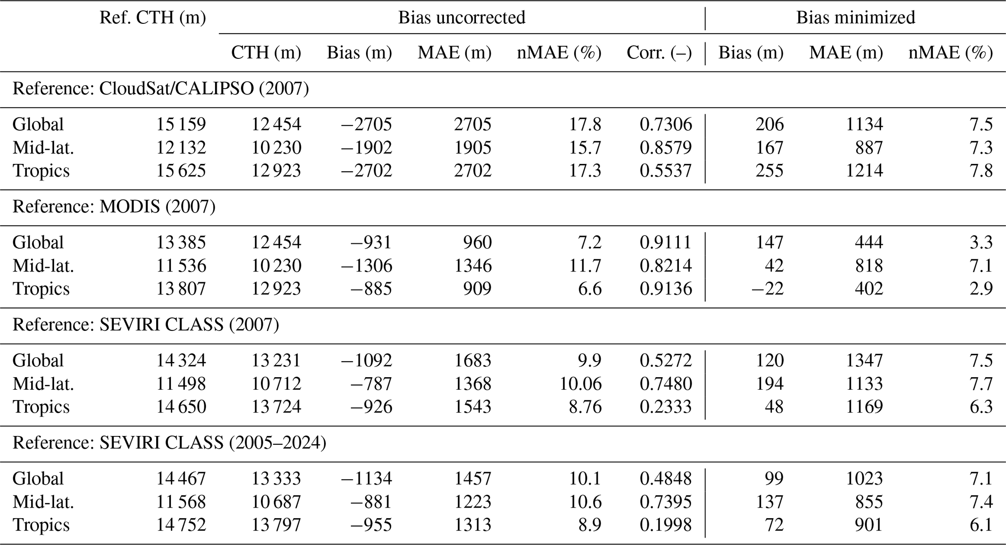
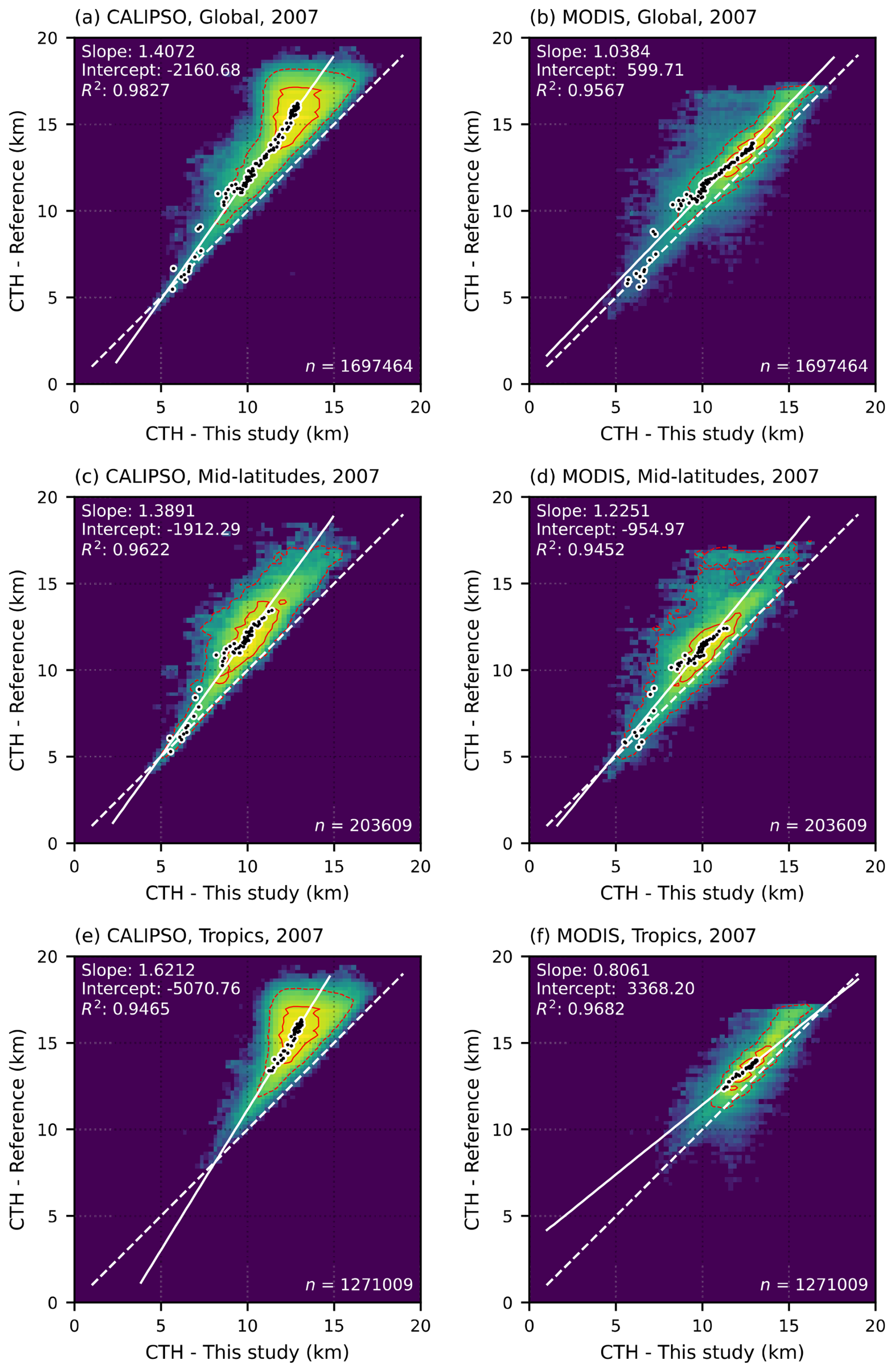
Figure 1 Cloud top height (CTH) estimated using the method developed in this study and reference data from CloudSat/CALIPSO (a, c, e) and MODIS (b, d, f) for the global domain excluding the polar regions (a, b), the mid-latitudes (c, d), and the tropics (e, f). Frequencies are shown on a logarithmic scale, with the solid red line enclosing 50 % of all cases and the dashed red line enclosing 95 % of cases. Black dots represent CTH averaged over 1° latitude bands to account for the significant latitudinal disproportions in DCC occurrence. The white line indicates the best linear fit (coefficients given in the top-left corner) to the zonally averaged CTH estimates (R² applies to the zonally averaged means).

Evaluation against MODIS showed a noticeably higher degree of agreement (Fig. 1b), according to almost all statistical measures considered. On a global scale, the bias decreased threefold (to −0.9 km), as did the mean relative error (to 1.0 km), and the normalized error (to 7 %). Agreement in the tropics and mid-latitudes also improved; however the tendency reversed compared with the validation against CloudSat/CALIPSO, with the tropics showing higher correlation (0.9136) and lower bias (−0.9 km) than the mid-latitudes (0.8214 and −1.3 km, respectively).

The better agreement with MODIS results from the known underestimation of CTH by that dataset, which arises from its radiative retrieval method. CO₂/IRW and other radiative-based approaches have been validated against CloudSat/CALIPSO and consistently reveal underperformance relative to direct lidar–radar measurements. It is important to note that cloud-top pressure retrieval using the MODIS CO₂/IRW technique is accurate to 50 hPa (Hawkinson et al., 2005) corresponding to ∼1.0 km at 20 km altitude, or ∼0.5 km at 6–7 km altitude.

Holz et al. (2008) reported a global CTH bias of −1.4 km for MODIS Collection 5 for all cloud types. When only clouds with tops above 5 km were considered (including cirrus), the bias increased to −4 km. Similar research by Wang et al. (2016) showed that MODIS Collection 6 also underestimates CTH for high clouds, regardless of optical depth. In the present study, the MODIS–CloudSat/CALIPSO comparison was limited exclusively to DCCs, revealing a global CTH underestimation of −1.7 km by the radiative retrieval approach (−0.6 km in mid-latitudes and −1.8 km in the tropics), which is in line with previous studies.

The general tendency of radiative retrieval methods to underestimate CTH for clouds with tops above 5 km, and overestimate it for lower clouds has also been reported for other sensors. For instance, various CTH products derived from the VIIRS indicate cloud tops lower than those in the CloudSat/CALIPSO dataset by 1.5 km (Hawkinson et al., 2005), 0.7–1.3 km (Liu et al., 2025), or 1 km for clouds with emissivity greater than 0.8 (Li et al., 2020). Di Michele et al. (2013) reported a similar pattern for Atmospheric Infrared Sounder (AIRS) observations collocated with CALIPSO, identifying an approximately −3 km bias for clouds with tops near 15 km.

The VŠ24 retrieval method evaluated in this study underestimates CTH not only relative to CloudSat/CALIPSO, but also relative to MODIS, which itself tends to underestimate CTH due to its radiative retrieval approach. Specifically, the method assumes that 11 µm BT represents the actual cloud-top temperature (CTT). However, when compared with operational MODIS CTT retrievals, 11 µm BT was on average 2.4 K higher than CTT, indicating that the at-sensor signal from the cloud top represents a mix of cloud-top radiance and radiance emitted by warmer atmospheric layers below the cloud top. A difference of 2.4 K corresponds to a change in CTH of ∼370 m in the troposphere under a standard lapse rate of 6.5 K km⁻¹, but this difference can increase to more than 1–2 km near the tropopause, where the lapse rate approaches zero and may become negative.

The bias increased with altitude in the validation against CloudSat/CALIPSO (Fig. 1a) and was also evident in the validation with MODIS over mid-latitudes (Fig. 1d). Since lidar–radar observations provide direct measurements of CTH, they are considered more reliable; therefore, validation against this dataset should be regarded as the most representative assessment of the true performance of the VŠ24 method.

The relationship between the reference and VŠ24-estimated CTH can be described using a simple regression model. Figure 1 shows the best linear fit between the two datasets. Since the frequency of DCCs varies considerably both between and within regions, the regression was performed not on individual CTH pairs, but on pairs of mean CTH values calculated within 1° latitude zones (black dots in Fig. 1).

Assuming an adequate goodness of fit, CTH estimates can be empirically adjusted. In this study the adjustment procedure relied on first order polynomial fit (white line on Fig. 1): VŠ24 CTH estimates were scaled by polynomial “slope” parameter, and then added to polynomial “intercept” parameter. As a result, bias-adjusted estimates can be obtained, and comparison with the reference dataset shows a substantial improvement in agreement (Table 1). The bias is reduced to 20–250 m, depending on the region and reference dataset. Likewise, the mean absolute error and normalized error decrease by approximately half, reaching 0.4–1.2 km and 2 %–8 %, respectively. These results demonstrate that calibration against a reliable reference dataset can significantly improve the accuracy of the VŠ24 method.

Because this calibration is a first-order (affine) transform, it is monotonic and one-to-one: it rescales and shifts the retrieved values but cannot create, suppress, or reorder features in the underlying field. Any trend or spatial gradient in the raw CTH is therefore preserved in sign and only rescaled; as the fitted slopes are ≥1, the adjustment amplifies rather than dampens CTH variability, and so cannot smooth out a genuine physical signal. Since the linear calibration coefficients were derived from a relatively short reference period, they may not fully generalise to other seasons. Therefore, any operational application of this approach should consider recalibrating over a longer period. Given this limitation, the core discussion in the remainder of the text focuses on the “raw” (non-adjusted) retrievals, which are free from this constraint.

4.2 Validation with Meteosat

While A-Train sensors provide a favourable nadir-viewing geometry, geostationary sensors operate across a wide range of viewing angles. Across most of the Earth's disc, clouds are observed progressively more from the side as the satellite zenith angle (SZA) increases toward the limb. While the term “cloud top” is still used, it is important to note that at-sensor radiance at high SZAs includes contributions from cloud sides. To mitigate these geometric effects, all Meteosat pixels with SZA>70° were excluded from the analysis.

The height of DCC tops estimated using the VŠ24 method was, on average, 1.1 km lower than that retrieved from SEVIRI-based CLAAS data. The mean absolute error was 1.5 km, corresponding to a normalized error of 10 % (Table 1). Overall, the systematic underestimation of CTH is consistent with tendencies previously reported for A-Train sensors, with agreement metrics falling between those obtained for MODIS and CloudSat/CALIPSO validations. Nevertheless, two notable exceptions were identified.

First, a substantially larger fraction of cases was observed in which DCC top heights estimated using the VŠ24 method were higher than the CTH reported by CLAAS (points located below the one-to-one line in Fig. 2). Although these situations represent a minority (17.2 %) of all observations, they occur far more frequently with SEVIRI than in comparisons with MODIS (<3.8 %), and are nearly absent in evaluations against CloudSat/CALIPSO (0.1 %). Occasionally, the overestimation reached up to 10 km. Second, validation against CLAAS in the tropics reduced performance in terms of correlation, with coefficients below 0.2. This contrasts with correlations of ∼0.5 obtained for CloudSat/CALIPSO and ∼0.9 for MODIS.

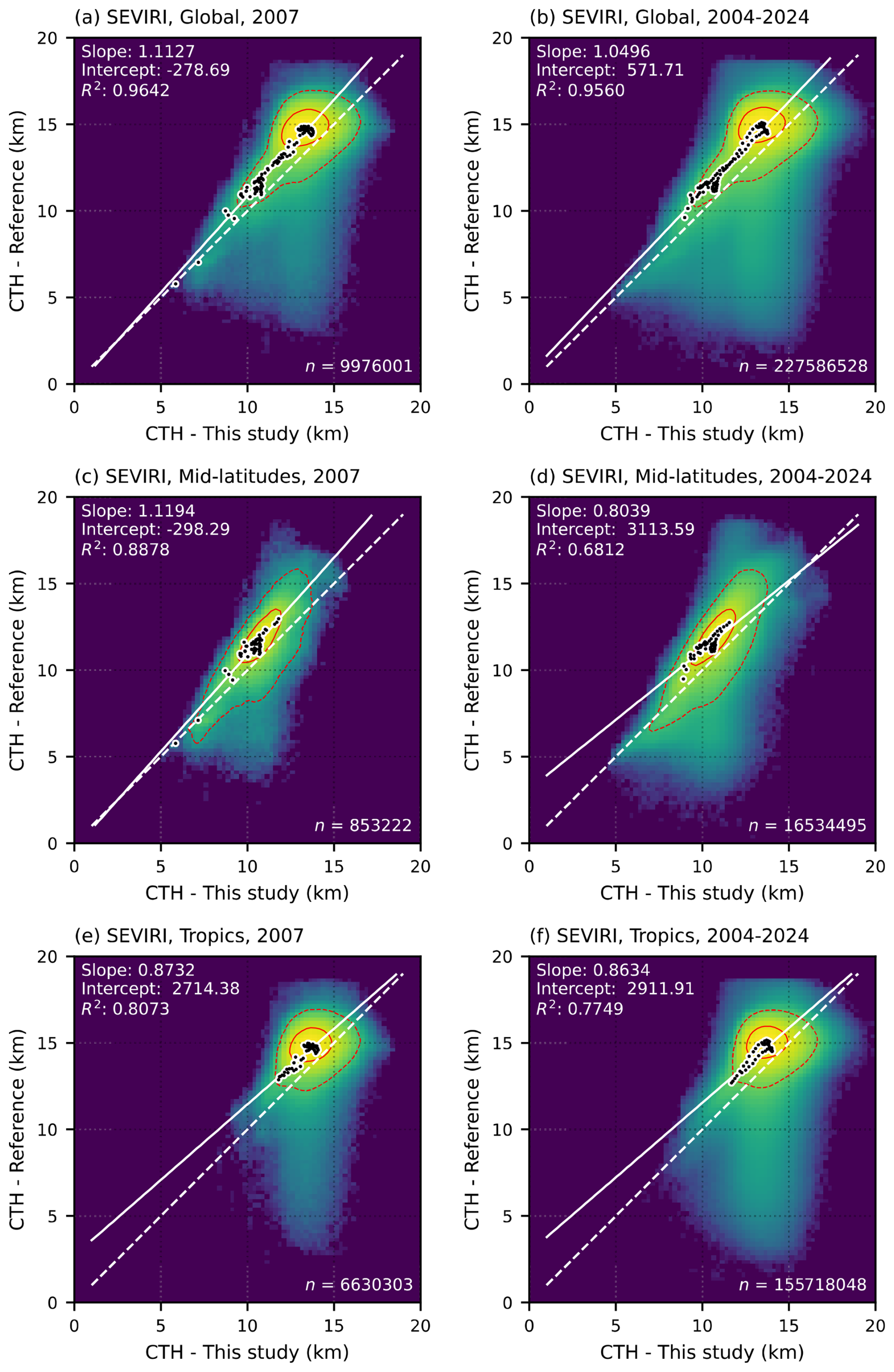
Figure 2 Cloud top height (CTH) estimated using the method developed in this study and reference data from SEVIRI CLAAS-3 dataset for year 2007 (a, c, e) and 2004–2024 (b, d, f) for the global domain excluding the polar regions (a, b), the mid-latitudes (c, d), and the tropics (e, f). Frequencies are shown on a logarithmic scale, with the solid red line enclosing 50 % of all cases and the dashed red line enclosing 95 % of cases. Black dots represent CTH averaged over 1° latitude bands to account for the significant latitudinal disproportions in DCC occurrence. The white line indicates the best linear fit (coefficients given in the top-left corner) to the zonally averaged CTH estimates (R² applies to the zonally averaged means).

In both cases, higher discrepancies may arise either from limitations of the VŠ24 retrieval method or from uncertainties in the CLAAS CTH algorithm. Since comparable issues were not observed in validations against MODIS or CloudSat/CALIPSO, deficiencies in the CLAAS product may be the more probable explanation. However, because both CLAAS and the VŠ24 method rely on the same SEVIRI observations, and are similarly affected by viewing-geometry constraints, either retrieval – or a combination of both – may contribute to the observed disagreement.

The observed estimation errors are consistent with those reported by Hamann et al. (2014), who performed a simultaneous validation of ten SEVIRI CTH retrieval algorithms using collocated lidar and radar observations. Validation against lidar alone revealed a systematic underestimation of CTH, ranging from 1 to 2.5 km (1.7 km on average) for all cloud types, with the bias increasing to 2–4 km at altitudes ∼15 km. Independent validation using CloudSat, which is less sensitive to optically thin clouds and thus reduces potential contamination from cirrus above DCCs, showed a similar tendency, with underestimation of 1–2 km for clouds with tops between 10 and 15 km.

Validation specifically targeting CLAAS version 3 (Benas et al., 2023) and conducted using CALIPSO lidar also reported systematic underestimation of SEVIRI CTH: less than 1 km globally for all cloud types, and 1–4 km for clouds within the Intertropical Convergence Zone. Benas et al. (2023) suggested that these errors may be associated with DCCs and related cirrus outflow, although no cloud-type-specific statistics were provided. Underestimation of comparable magnitude has also been reported for other geostationary imagers validated against CloudSat and CALIPSO, for example up to 2 km at 15 km altitude for Himawari-8 (Huang et al., 2019) and 2–3 km at the same altitude for FY-4A (Tan et al., 2019). As in the case of MODIS, VŠ24-based estimates validated in this study show CTH underestimation with respect to the CLAAS dataset, which itself underestimates CTH with respect to direct lidar measurements.

The CLAAS CTH product provides not only cloud-top height estimates, but also pixel-level uncertainty measures. For the DCCs analysed here, the average half-width of the uncertainty range was 1.0 km globally and in the tropics, and 0.8 km in mid-latitudes. These uncertainty estimates were used to assess whether CTH values derived with the VŠ24 method fell within the CLAAS uncertainty range. At the global scale, 64 % of retrievals satisfied this criterion, while 14 % exceeded the upper bound and 22 % fell below the lower bound. When analysed separately, 53 %–57 % of observations in the tropics and mid-latitudes were within the uncertainty range, 33 %–39 % fell below the lower bound, and 8 %–9 % exceeded the upper bound.

5 Application to parallax correction

The primary objective of this study is to evaluate the computationally efficient CTH estimation method proposed by VŠ24 for use in parallax correction of geostationary satellite imagery. The approach is assessed using SEVIRI data for the Northern Hemisphere summer of 2005 (June–August) over a pan-European domain (30–70° N, 15° W–40° E). Parallax corrections were computed using the Python package Satpy (version 0.55.0), part of the PyTroll data-processing framework (Raspaud et al., 2018).

CloudSat/CALIPSO lidar–radar profiles provide the least biased, near-absolute CTH reference and are used as such in Sect. 4.1; they cannot, however, anchor the parallax-correction step itself. Their nadir-only, sub-kilometre swath samples the European domain too sparsely to build a spatially complete parallax field, and it does not reproduce the large, SZA-dependent viewing geometry that characterises geostationary observations and that parallax correction must address. The operative question here is practical – how closely the VŠ24 retrieval reproduces the parallax correction actually applied to SEVIRI in operations – so the operational geostationary product for this platform, CLAAS-3, is the natural benchmark, used as a reference and never as ground truth (a term we deliberately avoid). CLAAS-3 carries its own retrieval uncertainty, which EUMETSAT provides per pixel and which we propagate throughout, assessing agreement not only against the central CLAAS-3 estimate but also against its uncertainty range. Optimal performance is achieved when the parallax displacements derived from the VŠ24 method closely match those of the CLAAS reference.

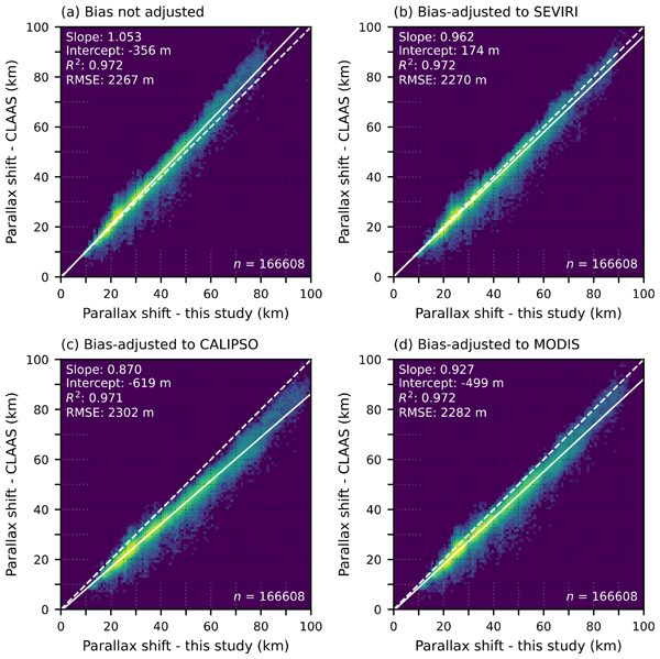
Four variants of CTH input were evaluated. The baseline configuration corresponds to the raw, unadjusted CTH estimates, with no bias correction applied. The remaining three variants were bias-adjusted using linear regression relationships (Figs. 1 and 2) derived against CTH from CloudSat/CALIPSO, MODIS, and SEVIRI, respectively.

5.1 Parallax shift vectors

According to the CLAAS reference data (Table 2), the mean displacement vector length for DCC tops over Europe in summer 2005 was 32.5 km, with a standard deviation of 13.6 km. The evaluated configuration of the VŠ24 method tends to underestimate CTH; it therefore systematically produces lower cloud tops and consequently shorter parallax displacement vectors. For the unadjusted version, the mean displacement was 1.3 km shorter than that derived from CLAAS (Fig. 3a). The corresponding mean absolute error was approximately 2.0 km, equivalent to a normalized mean absolute error of 6.0 %.

Table 2 Length of the parallax shift vector calculated using CTH derived from the Šoljan et al. (2024) method (“Est.”), compared to vectors obtained using SEVIRI CLAAS-3 CTH estimates (“Ref.”). The tested datasets are in unadjusted form (i.e., no bias adjustments applied to CTH estimates) and in forms adjusted to CloudSat/CALIPSO, MODIS, or SEVIRI CTH data.

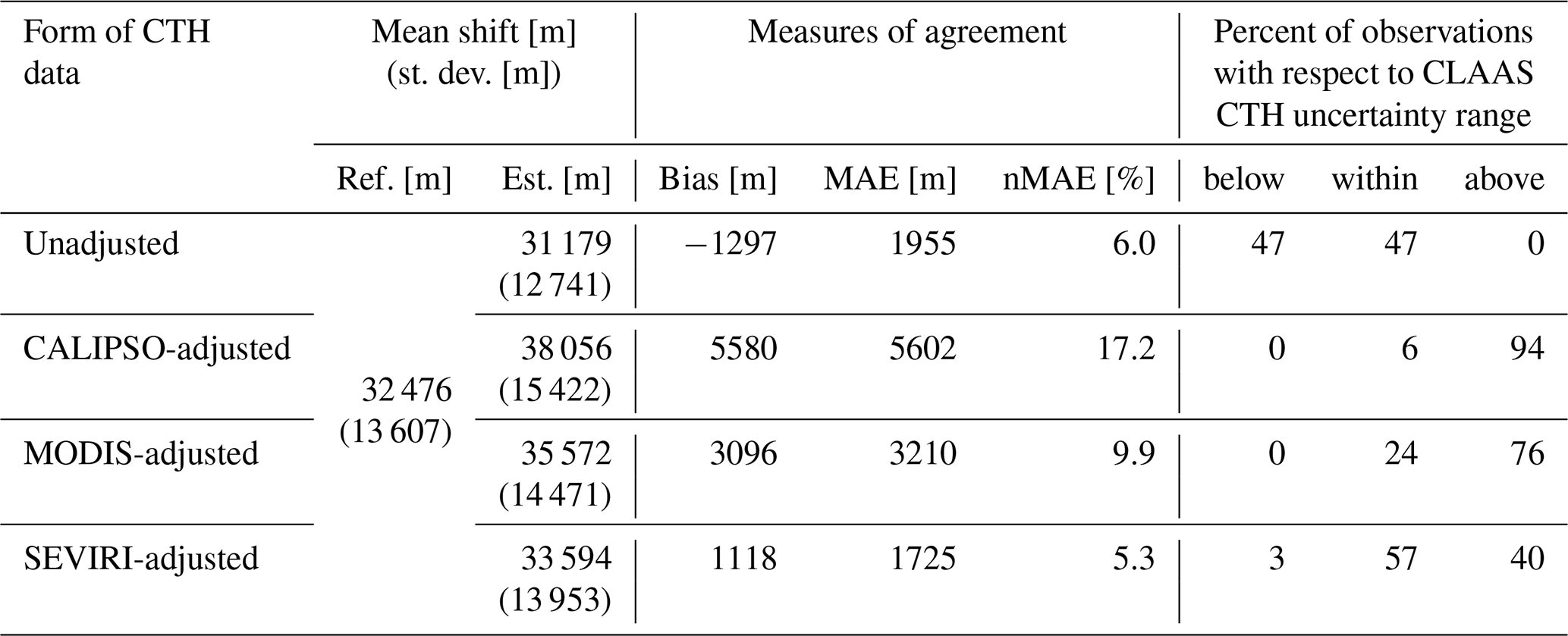
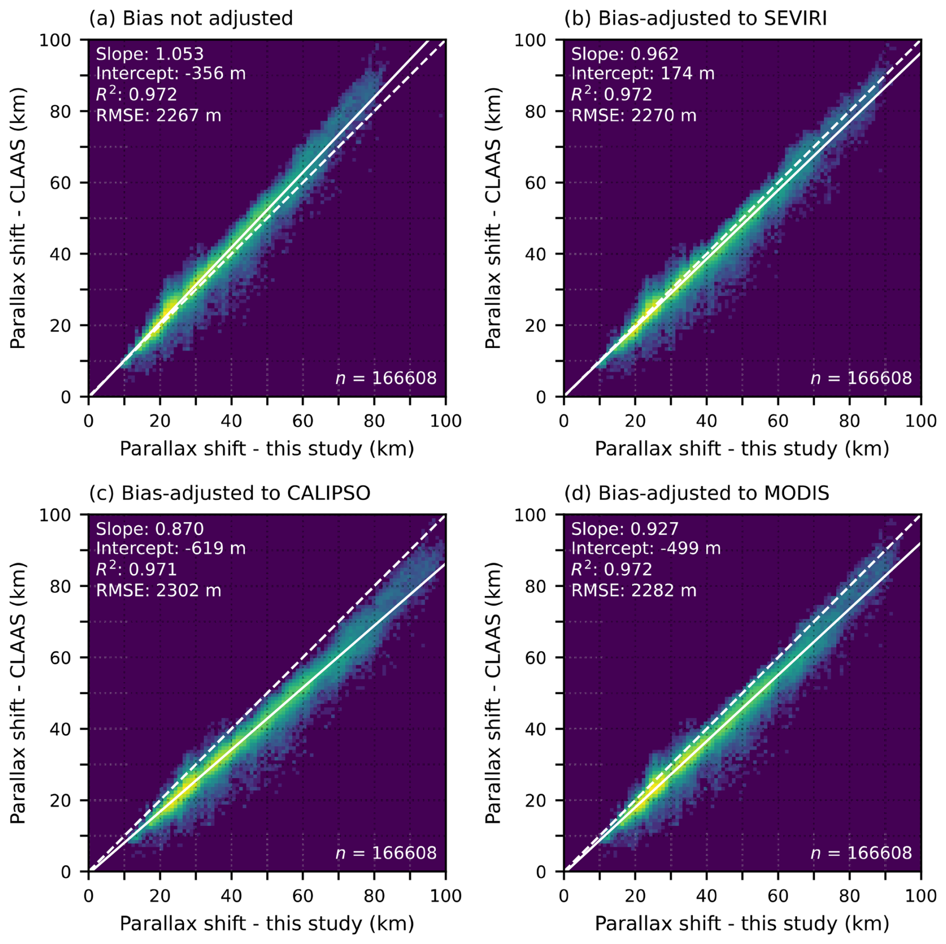
Figure 3 Length (in kilometres) of the parallax shift vector for DCCs over Europe in summer (June–July–August) 2005, as estimated using reference data from CLAAS and variants of CTH retrieved with this study's method: bias unadjusted (a); bias adjusted to match SEVIRI (b), CloudSat/CALIPSO (c), and MODIS (d).

The SEVIRI bias-adjusted version of the VŠ24 CTH retrieval yielded results very similar to the unadjusted configuration. The mean absolute error decreased marginally by 0.2 km, and the relative error decreased slightly to 5.3 %. In this case, the mean displacement was 1.1 km longer than the CLAAS-based estimate. As illustrated in Fig. 3a and b, the SEVIRI-adjusted and unadjusted versions produce highly consistent results, with only a modest improvement in performance for the adjusted configuration.

In contrast, bias adjustment to MODIS and CloudSat/CALIPSO noticeably increased the retrieved CTH, leading to systematically longer parallax displacement vectors. Relative to the CLAAS-based calculations, the MODIS-adjusted vectors were on average 3.0 km longer, while those adjusted to CloudSat/CALIPSO were longer by 5.6 km. Because the MODIS- and CloudSat/CALIPSO-based vectors were predominantly longer than the CLAAS reference, the mean absolute error remained of comparable magnitude. However, the relative error increased to 9.9 % for MODIS and 17.2 % for CloudSat/CALIPSO, reflecting the systematic tendency of these datasets to report higher CTH values.

5.2 Pixel-level displacement

From a practical perspective, errors in vector length can be tolerated provided they do not affect the final pixel assignment of the parallax-corrected data. The pixel-equivalent shift depends on the SZA. For example, a 10 km shift vector at a near-nadir location with an imaging resolution of 3 km per pixel may correspond to a displacement of 3–4 pixels. In contrast, at larger viewing angles (i.e., farther from nadir), the same metric shift may remain within a single pixel, resulting in no effective change in the data location after parallax correction.

Spatial resolution therefore plays a role in mitigating CTH estimation errors in the context of parallax correction, although the degree of mitigation is strongly resolution-dependent. Lower agreement is expected at finer spatial resolutions, because a given displacement vector spans a smaller number of pixels. Consequently, better agreement can be expected for coarser-resolution grids, or satellites with a larger field of view. For SEVIRI infrared channel data, the spatial resolution is 3 km per pixel at nadir. Using this value, it is possible to quantify how many pixels were reassigned to the same image location – that is, the same row and column in the SEVIRI image – when parallax correction was applied using CLAAS-based CTH versus VŠ24-based CTH estimates.

The results show that parallax correction using the unadjusted variant of the VŠ24 method placed 84 % of DCC pixels in the same location as the CLAAS-based correction, with the SEVIRI-adjusted variant yielding nearly identical agreement (82 %). Agreement decreased substantially for the MODIS-adjusted variant (58 %) and more markedly for the CloudSat/CALIPSO-adjusted variant (21 %). Given that the bias adjustment was trained on SEVIRI data, the resulting regression formula may not be fully transferable to earlier Meteosat observations (MVIRI sensors). However, it should be emphasised that the high 84 % agreement was achieved for the unadjusted scenario, which relies solely on ERA5 parameters – independent of Meteosat generation – and requires no a priori information about any regression functions.

When the uncertainty in CLAAS CTH estimates was taken into account, agreement exceeded 80 % in all cases and improved considerably across all variants. Under this assumption, 96.7 % of pixels in the unadjusted variant were assigned to the same location as with CLAAS, compared to 95.1 % for the SEVIRI-adjusted variant. Agreement also improved for the MODIS-adjusted (74.0 %) and CloudSat/CALIPSO-adjusted (37.0 %) variants.

It should be noted that the parallax correction evaluated here is assessed against CLAAS-based corrections, i.e. one retrieval is compared with another, rather than with an observed cloud displacement. Since parallax correction is a deterministic geometric transformation in which CTH is the only uncertain input, its accuracy is inherited directly from the CTH validation against CloudSat/CALIPSO (Sect. 4.1); independent verification against surface-based signatures of convection remains a valuable, though non-trivial, direction for future work, as such signatures mark the convective core rather than the cloud top.

5.3 Impact on DCC climatology

It is also important to assess how sensitive DCC climatology is to uncertainties in DCC location arising from parallax errors associated with CTH estimation. For this purpose, the reference dataset consists of mean monthly and seasonal DCC frequencies calculated using CLAAS-based parallax correction. Comparable DCC frequency statistics were then computed using parallax correction with VŠ24-based CTH data, considering both the unadjusted CTH and the three bias-adjusted variants. For additional comparison, DCC statistics derived from SEVIRI observations without parallax correction were also included. DCC frequencies are reported on a 0–1 scale, where 0 indicates that a DCC was never observed, and 1 indicates that a DCC was observed in every SEVIRI scan.

The monthly average DCC frequency over Europe in summer 2005 was approximately 0.007, with some locations reaching 0.04–0.06 (95th percentile), which is consistent with previous estimates of DCC occurrence in mid-latitudes (Pfister et al., 2022; Rossow and Schiffer, 1999). The results indicate that parallax correction itself is a significant factor in calculating DCC climatology. The difference in DCC frequency between CLAAS-corrected data and uncorrected data was 0.00066 seasonally and approximately 0.0014 monthly. While small in absolute terms, this difference corresponds to a normalized absolute error of 13 % on a seasonal scale, and 20 % on a monthly scale (Table 3).

Table 3 Seasonal (June–July–August) and monthly mean frequency of deep convective clouds (DCC). Statistics reported for datasets using unadjusted CTH estimates (i.e., no bias adjustments applied to CTH estimates) and adjusted to CloudSat/CALIPSO, MODIS, or SEVIRI CTH data. Errors (MAE, nMAE) are reported with respect to the DCC frequency calculated from data corrected for parallax effects using the SEVIRI CLAAS-3 product.

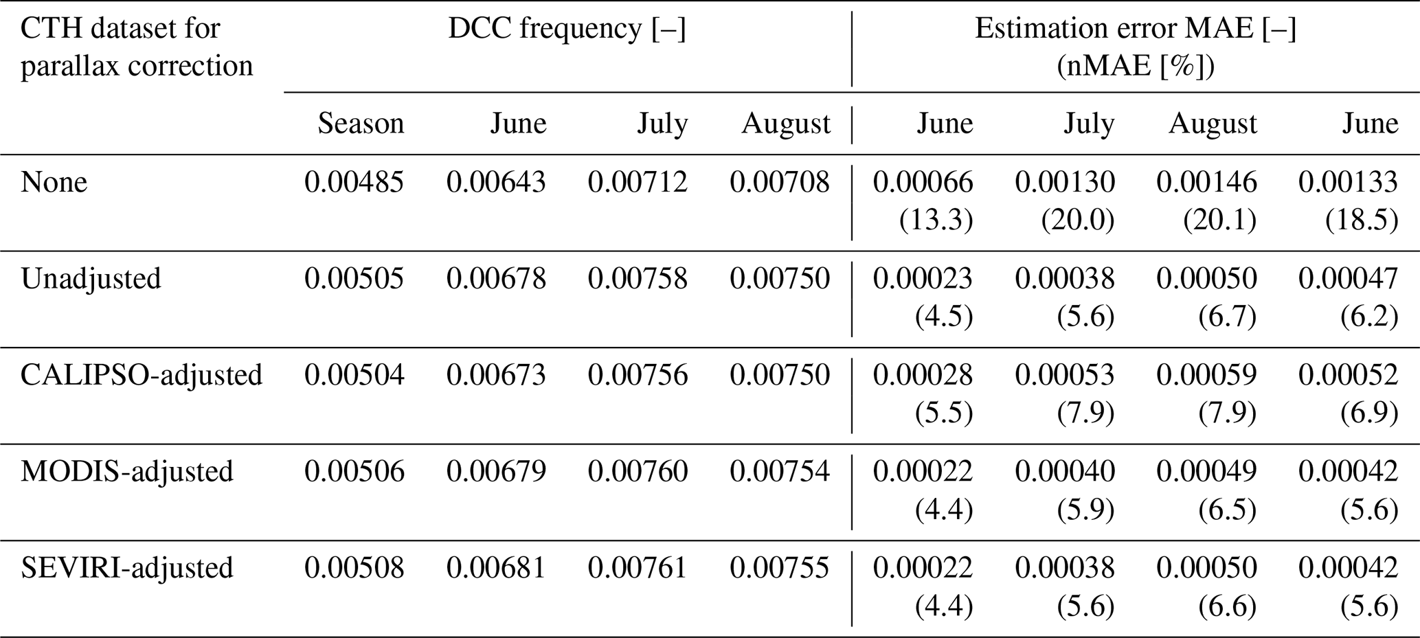
Discrepancies relative to the CLAAS-based data decreased substantially when VŠ24-based CTH was applied, compared with the no-parallax-correction scenario. Using the unadjusted variant, the mean absolute difference in DCC frequency decreased to 0.00023 seasonally and 0.0004–0.0005 monthly, corresponding to normalized errors of 5 % and 6 %–7 %, respectively. Similar results were observed for the SEVIRI-adjusted variant, consistent with previous findings (Table 3). Among all variants, the SEVIRI-adjusted dataset showed the closest agreement with the CLAAS-based reference (seasonal normalized errors of 5.6 %–6.6 %), followed closely by the MODIS-adjusted variant, while the CloudSat/CALIPSO-adjusted variant performed least accurately (6.9 %–7.9 %).

6 Summary and conclusions

Cloud-top height (CTH) is a key atmospheric parameter and a critical input for parallax correction, a procedure that, if neglected, can introduce substantial errors into DCC climatologies, as demonstrated in this study. Efficient processing of large volumes of multidecadal remote sensing data requires a fast and reliable CTH estimation method that relies solely on the limited radiometric information available from early meteorological satellites.

This study evaluated the CTH estimation method developed by Šoljan et al. (2024), which is based on the well-established concept of matching cloud-top BT in a single infrared window channel (11 µm) with an atmospheric temperature profile. The method employs a non-iterative approximation of the moist adiabat (pseudoadiabat) and can be applied globally using three standard meteorological parameters: dew point temperature, air temperature, and air pressure, available from numerical weather prediction models or reanalyses. The effectiveness of the Šoljan et al. (2024) method was validated in the context of parallax correction against three operational CTH products: MODIS, CloudSat/CALIPSO, and SEVIRI CLAAS.

Specifically, this study addressed whether the Šoljan et al. (2024) method is a viable alternative to existing operational approaches. The results demonstrate that:

• the VŠ24 method is sufficiently accurate for CTH estimation of DCCs and represents a viable alternative to the operational SEVIRI CLAAS product. Although it underestimated CTH relative to CLAAS by approximately 10 %, this bias did not significantly affect the resulting parallax correction. Approximately 84 % of pixel geolocations were consistent between VŠ24-based and CLAAS-based parallax corrections, increasing to 97 % when CLAAS retrieval uncertainty was accounted for. Errors in DCC frequency relative to CLAAS remained below 7 % on a monthly scale and below 5 % on a seasonal scale, with even smaller discrepancies expected on an annual scale;

• CTH estimates from the VŠ24 method correlated well with CloudSat/CALIPSO and MODIS data at the global scale (correlation coefficients of 0.7–0.9) and across mid-latitudes (0.7–0.8 across all reference datasets). These relationships were well captured by simple linear regression models (R²>0.9), enabling effective bias adjustment. After bias correction, CTH estimates showed normalized errors below 7 % relative to the reference datasets, corresponding to a mean absolute error of less than 1.2 km, consistent with typical uncertainties reported for infrared-based CTH retrievals.

The CTH estimation method of Šoljan et al. (2024) can be readily implemented on any polar-orbiting or geostationary platform equipped with an infrared window channel. Since this channel has been a standard feature of cloud imagers aboard meteorological satellites, the method enables the construction of homogeneous long-term datasets of DCCs (in terms of consistent parallax correction), facilitating its application across all generations of Meteosat satellites and other geostationary platform families.