Long-term climatology of vertical profiles of polarimetric variables and ice-microphysical retrievals at X-band – Part 1: Radar calibration

In a two-part series of papers, a climatology of quasi-vertical profiles (QVPs) of polarimetric variables and ice-microphysical retrievals such as ice water content, total number concentration and mean volume diameter is presented. QVPs are generated from plan position indicator scans at 18° elevation angle measured with the X-band radar located in the city of Bonn in western Germany between 2013 and 2023. They have been statistically analysed including error analysis with special emphasis on the characteristics of the melting layer and the dendritic growth layer. This long-term climatology improves the understanding of microphysical processes in stratiform cloud regimes and provides a reference for numerical weather prediction modellers to e.g. advance existing microphysical bulk paramerisation schemes.

While part two analyses and discusses the climatology, this first part of the series describes the prior thorough calibration of the radar reflectivity factor (Z_H) and the differential reflectivity (Z_DR). One method uses the relation between Z_H and Z_DR in light rain to calibrate Z_H. Best fits are determined from simulated Z_H and Z_DR values obtained with T-matrix calculations for various temperatures and values of the width of the canting angle distribution using a large disdrometer dataset of drop size distributions measured over Germany (mostly Bonn). Since this Z_H calibration technique strongly depends on the accuracy of Z_DR and encountered deficiencies in the birdbath scan, QVPs in light rain have been used to calibrate Z_DR. Obtained Z_H offset values are validated and compared using both satellite information and self-consistency relationships including specific differential phase (K_DP). The successful calibration of Z_H is confirmed by the root-mean-square error (0.70 dB), the mean-absolute error (0.60 dB), and the mean-bias (−0.50 dB) compared to the offsets obtained from satellite information. Offsets calculated by applying self-consistency relations show larger discrepancies, which favours the suitability of the novel method.

1 Introduction

Numerical weather prediction (NWP) models generally struggle with limitations of existing parameterisation schemes to adequately capture the complexity of microphysical processes (Ryzhkov et al., 2020; Fan et al., 2017). Since polarimetric radars enable us to distinguish between hydrometeors with different microphysical properties and/or habits (e.g. shape and number concentration) and to identify so-called polarimetric fingerprints indicating ongoing dominating microphysical processes like e.g. aggregation, size sorting or dendritic growth (Ryzhkov et al., 2016; Trömel et al., 2019; Kumjian, 2013a; Kumjian and Ryzhkov, 2010, among others), they can serve as a powerful tool for improving NWP parameterisation schemes and cloud models (Kennedy and Rutledge, 2011; Ryzhkov et al., 2020). The fusion of radar polarimetry and atmospheric modelling is a promising pathway to improve the representation of clouds and precipitation in NWP (Trömel et al., 2021). Using observation- (forward) operators (Kumjian and Ryzhkov, 2012; Ryzhkov et al., 2020), such as the Efficient Modular VOlume scan RADar Operator (EMVORADO; Zeng et al., 2016; Blahak, 2016; Blahak and de Lozar, 2021), synthetic polarimetric variables can be calculated from simulated hydrometeor mass fractions and number concentrations of NWP models and directly compared with observed polarimetric variables (e.g. on the radar grid; Trömel et al., 2023; Shrestha et al., 2022; Xie et al., 2021). E.g., with a detailed model evaluation in radar observation space, Shrestha et al. (2022) identified excessive graupel production in the COnsortium for Small scale MOdeling (COSMO) model (Doms and Baldauf, 2018; Doms et al., 2018) with the Seifert-Beheng two-moment microphysical parameterisation (SB2MP) scheme (Seifert and Beheng, 2006). To date, extensive graupel formation is still an ongoing challenge in many microphysical paramerisation schemes. Furthermore, model evaluation studies in radar observation space as well as polarimetric microphysical retrievals and in-situ observations show that existing NWP models coupled with various microphysical schemes tend to overestimate the size of aggregates and underestimate the number concentration of ice particles in general (e.g. Fridlind et al., 2017; Ori et al., 2020; Trömel et al., 2023, among others). Besides case studies, climatologies of polarimetric variables and microphysical retrievals are particularly important and serve as a statistically significant reference to understand and finally improve precipitation processes in atmospheric models.

In order to provide the required reliable information to NWP modelers, but also for most other radar applications in the scientific community and operational services, like quantitative precipitation estimation (QPE), nowcasting, hydrometeor classification and microphysical retrievals, precise calibration is a mandatory prerequisite (e.g. Ryzhkov and Zrnic, 2019; Warren et al., 2020; Houze Jr. et al., 2004; Crisologo, 2019). Although the use of novel gradient approaches (e.g. Planat et al., 2021) and phase-based measurements are gaining increased attention and popularity, it is unlikely that absolute values of the reflectivity factor Z_H and differential reflectivity Z_DR will ever become superfluous and instead will always remain a part of hybrid QPE and microphysical retrieval derivations. Calibration is also (even maybe to a lesser extent) relevant for climatologies in order to represent reality with sufficient accuracy and statistical significance by minimizing calibration induced uncertainties as much as possible. In principle, calibration induced uncertainties can be attributed to the characteristics of the receiver, transmitter, and, above all, the antenna, with the latter controlling the link between transmitted and received pulse power (e.g. Schneebeli et al., 2024).

Over the years, many techniques for calibrating Z_H and Z_DR have been developed and applied. Examples are the use of disdrometer data (e.g. Frech et al., 2017; Schneebeli et al., 2024; Frech, 2013), corner reflectors or metal spheres (attached on e.g. drones and balloons; e.g. Atlas and Mossop, 1960; Atlas, 2002; Williams et al., 2013; Ye et al., 2024; Joshil and Chandrasekar, 2022), virtually generated radar targets (Schneebeli et al., 2024; Wang et al., 2025; Schneebeli et al., 2025), solar signals (e.g. Frech and Hubbert, 2020; Holleman et al., 2010; Chu et al., 2019), stable ground clutter signals (e.g. Silberstein et al., 2008; Wolff et al., 2015; Pejcic et al., 2022; Hunzinger et al., 2020) or dominant point targets located close to the radar site (Gabella, 2018), self-consistency relations of polarimetric variables (e.g. Gorgucci et al., 1992; Louf et al., 2019; Gourley et al., 2009), Z_H−Z_DR dependencies in light rain (e.g. Ryzhkov and Zrnic, 2019), satellite (spaceborn) radar information (Pejcic et al., 2022; Louf et al., 2019; Louf and Protat, 2023; Crisologo et al., 2018), quasi-vertical profiles (QVPs; Ryzhkov et al., 2016) in light rain (Sanchez-Rivas and Rico-Ramirez, 2022), dry aggregated snow (e.g. Hu et al., 2026, 2024; Ryzhkov et al., 2005; Zittel et al., 2014), clear air Bragg scattering (e.g. Richardson et al., 2017), or the so-called birdbath scan method (e.g. Gorgucci et al., 1999; Frech and Hubbert, 2020; Louf et al., 2019; Ryzhkov and Zrnic, 2019; Pejcic et al., 2022; Sanchez-Rivas and Rico-Ramirez, 2022).

The latter exploits vertical scans, where raindrops appear nearly spherical to the radar, and is one of the most frequently used methods for accurate Z_DR calibration. Similarly, Z_DR is expected to be 0 dB when the radar is pointing towards the sun, due to the unpolarized nature of solar radiation in this direction. Monitoring the sun allows the detection potential receiver malfunctions or radar antenna misalignment (Holleman et al., 2010). To determine more precisely which components of the radar system are responsible for any system biases, the latter two techniques can be combined, as demonstrated in Figueras i Ventura et al. (2012). In particular, the difference between the Z_DR derived from solar signals and that obtained from birdbath scans can be used to identify transmitter biases.

The first part of the paper series focuses on the prior, as noted above, very important calibration of Z_DR and Z_H, while the second part deals with the description and the statistical analysis of the climatology of QVPs of polarimetric variables and ice-microphysical retrievals obtained from 10 years of X-band radar data measured in stratiform rain.

Most of the calibration methods briefly presented above are either not retrospectively applicable because e.g. the required scanning strategy is missing, the radar system is simply not capable of setting it up, the required measurements are not saved, or it is not possible to cover the whole time period. Although the birdbath method is widely used to calibrate Z_DR, the results were not reliable throughout the entire climatological period; In particular, the offset values obtained for 2014 appeared unrealistically small, limiting the usefulness of the calibrated Z_DR. Instead applying the birdbath scan, a modified method adapted from Sanchez-Rivas and Rico-Ramirez (2022) using QVPs in light rain is exploited for Z_DR calibration and a Z_H calibration technique applicable to the entire time series from 2013–2023 is presented. It uses the known Z_H−Z_DR dependency (Ryzhkov and Zrnic, 2019), but with Z_DR as a predictor for Z_H measured on PPI scans at 18° elevation angle. This calibration method of Z_H is validated and compared to Z_H offset values obtained from satellite measurements, provided for a 5.5 year subset by Pejcic et al. (2022) and self-consistency relations as described in e.g. Louf et al. (2019).

The paper is structured as follows: Section 2 shortly introduces most important technical information and scanning strategies of the used radar and describes the steps of phase processing in more detail. The following Sect. 3 explains the problems encountered when using the birdbath scan method to correct Z_DR and presents the above mentioned alternative Z_DR calibration method used in this study, followed by the novel Z_H calibration method, its validation and the comparison with the self-consistency relation. Section 4 summarizes the results, highlights deficiencies and identifies potential improvements for future studies.

2 Radar data

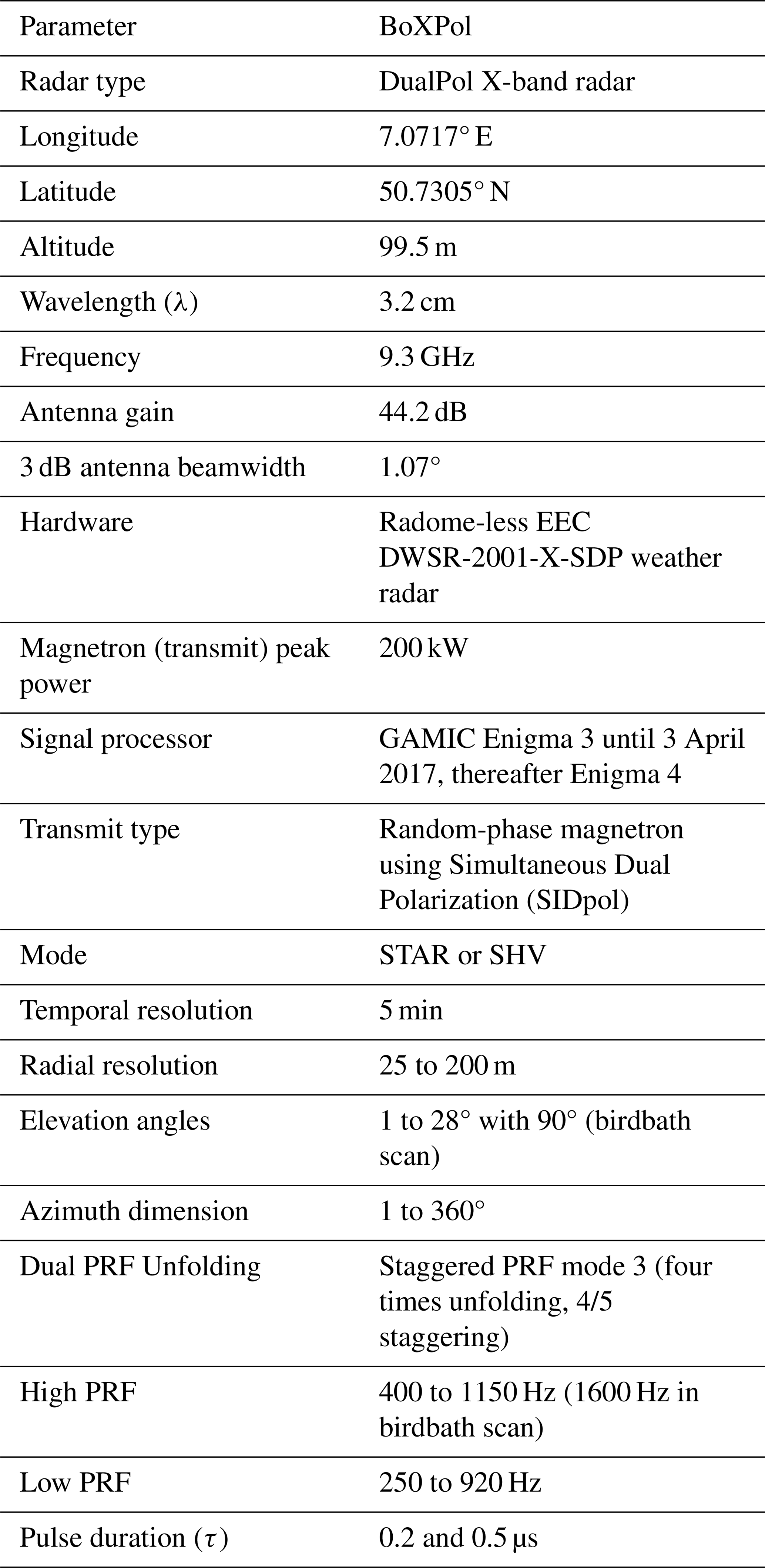
The radar data used in this study have been obtained with the polarimetric X-band radar in Bonn, Germany (BoXPol), located at 50.7305° N and 7.0717° E and 99.5 m above mean sea level (a.m.s.l). BoXPol measures within a radius of 100 km since 2009 (Fig. 1). The hardware includes an EEC DWSR-2001-X-SDP weather radar without a radome, operating in the simultaneous transmit and receive of horizontally and vertically polarized electromagnetic (EM)-waves (STAR or SHV) mode (Pejcic et al., 2022; Ryzhkov and Zrnic, 2019) using an Enigma signal processor. Plan position indicator (PPI) scans are generated at 10 different elevation angles, ranging from 1–28° and a (90°) birdbath scan in 5 min temporal and 1° azimuthal resolution. The range resolution depends on the chosen configuration of the elevation scan and ranges from 25–200 m. For the 18° elevation angle (used in this two paper series) it is 100 m until the third of April 2017 and afterwards 125 m, where Enigma 3 was updated to Enigma 4. BoXPol operates in dual pulse repetition frequency (PRF) unfolding (staggering) mode 3, with alternating low PRF and high PRF values in the azimuth dimension with values ranging from 400–1150 Hz (1600 Hz for the birdbath scan) and from 320–920 Hz, respectively, for various range resolutions (personal communication with Kai Mühlbauer, see also Table 2 in Pejcic et al., 2022). A range height indicator (RHI) scan is included in a 5 min scan schedule as well. For a more detailed information about the scanning strategies, reference is made to Diederich et al. (2015) or Pejcic et al. (2022).

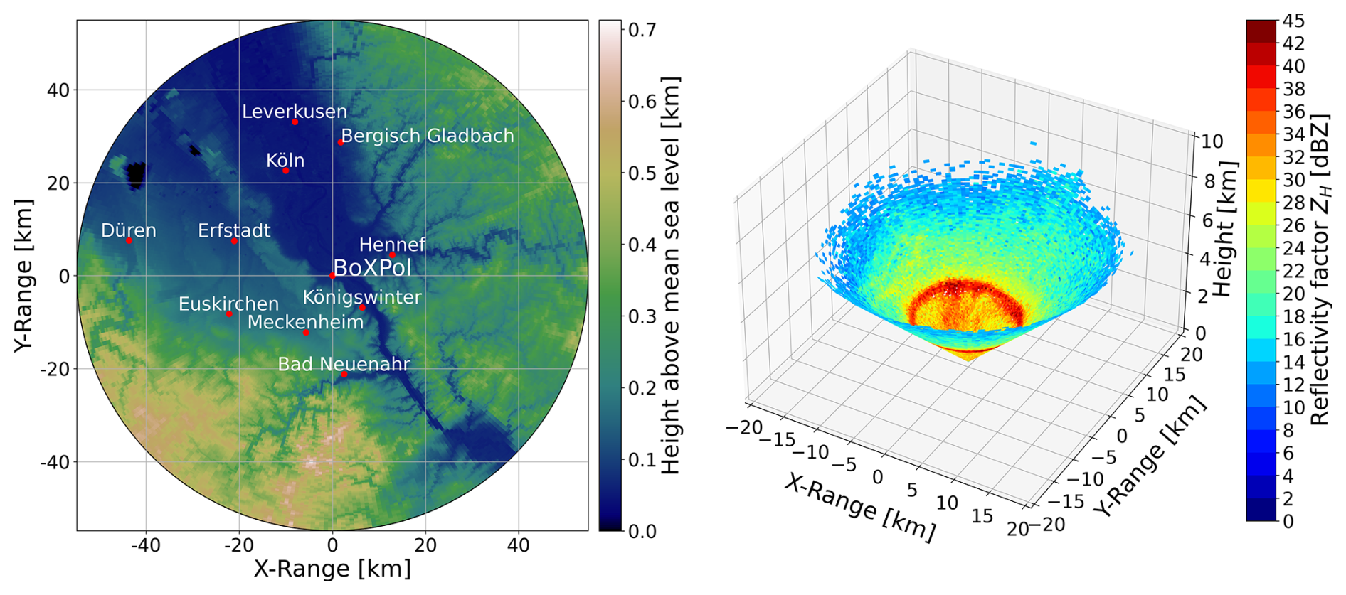
Figure 1 Location of BoXPol and covering area of the PPI scans at 18° elevation angle (550 km maximum range) including terrain height information and city names in the surrounding region given as red points (left). Example illustration of Z_H in a cone of the 18° PPI scan at the 7 October 2014, 00:00 UTC (right). Note that this figure represents the maximum range of BoXPol operating with Enigma 3 until the 4 March 2017.

All offset values (Z_DR and Z_H) are determined using PPI scans at 18° elevation angle. These measurements are also used in part 2 of this paper series for the climatology. The choice of this elevation angle represents a compromise: It already provides sufficient vertical profile information, but the use of even higher elevation angles would result in a significant degradation of the polarimetric information content. At angles below 20°, however, only slight acceptable decreases occur (Ryzhkov et al., 2005; Griffin et al., 2018; Trömel et al., 2019).

The height of the radar beam is calculated assuming $\mathrm{4}/\mathrm{3}$ effective earth radius (e.g., Doviak and Zrnić, 1993). No interpolation is applied, i.e. each range bin transforms into one height bin.

Table 1 Technical description of the X-band radar in Bonn (BoXPol).

Within the phase processing, first the system phase offset (${\mathit{\varphi }}_{\text{DP}}^{\text{sys}}$; Ryzhkov and Zrnic, 2019) has to be determined and subtracted from ϕ_DP. ${\mathit{\varphi }}_{\text{DP}}^{\text{sys}}$ is calculated by filtering with ρ_HV≥0.9 and Z_H≥0 and identifying the position of the first non-NaN measurement of ϕ_DP in each ray. Subsequently, the median of the values between this position and 3 km in the range dimension provide ${\mathit{\varphi }}_{\text{DP}}^{\text{sys}}$.

Afterwards, the offset-corrected ϕ_DP is smoothed using a moving median with a window length of 11 range bins. The specific differential phase (K_DP; e.g. Trömel et al., 2014; Ryzhkov and Zrnic, 2019; Vulpiani et al., 2012) in degrees per kilometer (° km⁻¹) is calculated applying low-noise Lanczos differentials (Holoborodko, 2015; Diekema and Koornwinder, 2012) implemented in ωradlib, using a window length of 31 range bins (corresponding to 3.1 km slant range for Enigma 3 and 3.875 km slant range for Enigma 4).

3 Calibration of Z_DR and Z_H

Assuming no specific attenuation (A_H; e.g. Kumjian, 2013b), wet radome effects (e.g. Le Loh et al., 2022) or noise influences (e.g. Schneebeli et al., 2024), a simple representation of the measured Z_H (e.g. Silberstein et al., 2008; Louf and Protat, 2023) based on the well-known radar equation (e.g.  Ryzhkov and Zrnic, 2019; Doviak and Zrnić, 1993; Rinehart, 1997), can be used to characterize possible calibration errors with the following equation:

$$\begin{array}{}\text{(1)}& \begin{array}{rl}& Z_{\mathrm{H}}=-\mathrm{10}{\log }_{\mathrm{10}}\\ & \times \underset{C_{\mathrm{r}}^{\mathrm{H}}}{\underbrace{\left({\displaystyle \frac{{\mathit{\pi }}^{\mathrm{3}}{\left|K_{\mathrm{w}}\right|}^{\mathrm{2}}}{{\mathit{\lambda }}^{\mathrm{2}}\times \mathrm{1024}\cdot \ln \mathrm{2}\times {\mathrm{10}}^{\mathrm{18}}}}{P}_{\mathrm{t}}^{\mathrm{H}}(G^{\mathrm{H}}{\mathit{\theta }}^{\mathrm{H}}{)}^{\mathrm{2}}c\mathit{\tau }{A}_{\mathrm{t}}^{\mathrm{H}}{A}_{\mathrm{r}}^{\mathrm{H}}\right)}}\\ & +\mathrm{20}{\log }_{\mathrm{10}}r+\mathrm{10}{\log }_{\mathrm{10}}{P}_{\mathrm{r}}^{\mathrm{H}}.\end{array}\end{array}$$

$P_{\mathrm{r}}^{\mathrm{H}}$ is the received and $P_{\mathrm{t}}^{\mathrm{H}}$ the transmitted power of the horizontal polarization channel in W, K_w is the dielectric factor of water, θ^H is the half power antenna beam width of the horizontal polarization channel in rad, c is the speed of light in ms⁻¹, G^H is the antenna gain of the horizontal polarization channel with the assumption that the antenna is for both transmitting and receiving, $A_{\mathrm{t}}^{\mathrm{H}}$ and $A_{\mathrm{r}}^{\mathrm{H}}$ are the transmitter and the receiver gains of the horizontal polarization channel, τ is the pulse duration of transmitted signals in s and r is the radial distance of the target in m.

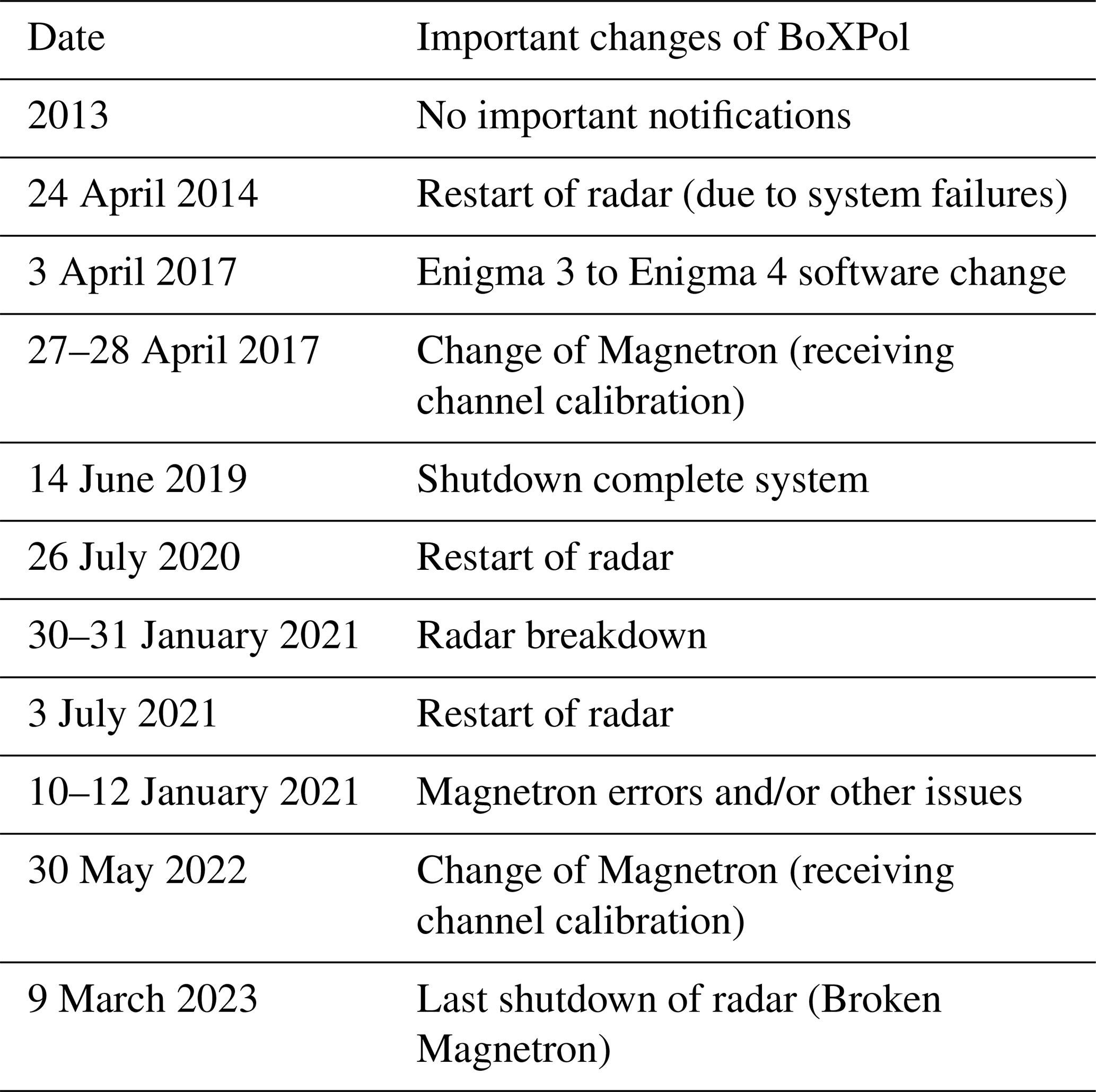
Table 2 Logbook of BoXPol displaying most important changes in hardware and software in the time period from January 2013–March 2023.

The underbraced term in Eq. (1) is the so-called radar constant of the horizontal channel $C_{\mathrm{r}}^{\mathrm{H}}$ (e.g. Schneebeli et al., 2024; Ryzhkov and Zrnic, 2019), which can vary over time and due to degradation of radar hardware (e.g. Louf et al., 2019) and represents the main source of potential calibration errors.

Similarly, Eq. (1) is valid for the reflectivity factor of the vertically polarized EM wave (Z_V) in the STAR mode, i.e. superscripts and subscripts “H” can be replaced by “V” (e.g. Ryzhkov and Zrnic, 2019; Schneebeli et al., 2024). As a result, any difference in the radar constants for both polarization channels may also result in a Z_DR miscalibration, as illustrated by the following equation:

$$\begin{array}{}\text{(2)}& Z_{\text{DR}}=\mathrm{10}{\log }_{\mathrm{10}}\left({\displaystyle \frac{P_{\mathrm{r}}^{\mathrm{H}}\cdot C_{\mathrm{r}}^{\mathrm{V}}}{P_{\mathrm{r}}^{\mathrm{V}}\cdot C_{\mathrm{r}}^{\mathrm{H}}}}\right).\end{array}$$

In the case of a perfectly calibrated (fictitious) radar (e.g. for the transmitter channel, for the receiver channel and for the antenna; Schneebeli et al., 2024), $C_{\mathrm{r}}^{\mathrm{H}}=C_{\mathrm{r}}^{\mathrm{V}}$ and thus, Z_DR depends on $P_{\mathrm{r}}^{\mathrm{V}}$ and $P_{\mathrm{r}}^{\mathrm{H}}$ only (e.g. Ryzhkov and Zrnic, 2019). Since a perfect internal calibration for the estimation of C_r is almost impossible, external sources/methods are mandatory for a sufficient calibration of Z_H and/or Z_DR² (Louf et al., 2019).

To enable quantitative applications like Quantitative Precipitation Estimation (QPE), microphysical retrievals or hydrometeor classification, Z_DR needs to be calibrated with an accuracy of 0.1–0.2 dB (Frech and Hubbert, 2020; Ryzhkov and Zrnic, 2019). As mentioned before, the birdbath (90° elevation angle) scan method is one of the most powerful calibration methods for Z_DR (Ryzhkov and Zrnic, 2019; Frech et al., 2017; Louf et al., 2019). Since the mean angle of incidence of raindrops is close to 0°, they appear spherical when viewed from below. This means that both Z_H and Z_V should be equal and deviations can be used for calibration of Z_DR in light rain (Ryzhkov and Zrnic, 2019). In this study, Z_DR offsets from the birdbath scan are calculated using a similar but slightly more rigorous procedure compared to Pejcic et al. (2022). First, mixed phase hydrometeors are excluded using only data at heights at least 250 m away from the 0 °C isotherm. The temperature information is taken from the European Center for Medium-Range Weather Forecasts Reanalysis v5 (ERA5; Hersbach et al., 2020). Afterwards, the median between the 20th and 80th percentiles of Z_DR is calculated (instead of the 10th and 90th percentiles in Pejcic et al., 2022), whereby only days with >100 non-NaN values and a standard deviation <0.2 dB are considered as reliable for estimating the daily Z_DR offset.

However, serious inconsistencies in the Z_DR offset values obtained using the birdbath scan method were discovered. While the method provided reliable offsets for the period between April 2014 and March 2017, inaccuracies of more than 0.2 dB were obtained for other times (especially for 2013 to early 2014). Due to various hardware and software changes between 2013 and 2023 documented in the BoXPol logbook (private communication with Kai Mühlbauer and Martin Lennefer, 6 March 2024, summarized in Table 2), such as the replacement of hardware components (e.g. Magnetron), software updates (Enigma 3 to Enigma 4), but also unfathomable influences, offsets derived from the birdbath scan seem not to be applicable to the 18° elevation PPI. These circumstances most likely lead to discrepancies in the components of C_r for both channels (see Eq. 2) and also may point to a potentially unsuspected elevation dependence. The ratios of the radar constants for the birdbath (BB) scan (C_r,BB) and the 18° elevation scan (C_r,18) of the horizontal (H) and vertical (V) polarization channels appear to deviate from each other:

$$\begin{array}{}\text{(3)}& {\displaystyle \frac{C_{\mathrm{r},\text{BB}}^{\mathrm{V}}}{C_{\mathrm{r},\text{BB}}^{\mathrm{H}}}}\ne {\displaystyle \frac{C_{\mathrm{r},\mathrm{18}}^{\mathrm{V}}}{C_{\mathrm{r},\mathrm{18}}^{\mathrm{H}}}}.\end{array}$$

This potential elevation dependence could be related either to the mechanical control of elevation angles in the BoXPol scanning strategy or to issues with the rotary joints between the transmitter/receiver and the antenna (private communication with Martin Lennefer and Kai Mühlbauer, 6 March 2024; Figueras i Ventura et al., 2012). Therefore, the QVPs themselves are used to calculate the Z_DR offset (Sanchez-Rivas and Rico-Ramirez, 2022) and to subsequently calibrate Z_H based on the offset corrected Z_DR.

In the following, Sect. 3.1 describes the Z_DR calibration technique and Sect. 3.2 the calibration of Z_H, while Sect. 3.2.1 and 3.2.2 compare and validate the results using self-consistency relations and satellite information.

3.1 Z_DR Calibration

Light rain conditions are identified with $\mathrm{0}<Z_{\mathrm{H}}<\mathrm{20}\mathrm{dBZ}$ and ρ_HV>0.985 (Sanchez-Rivas and Rico-Ramirez, 2022) and ϕ_DP<30°. The latter is a precautionary step intended to effectively exclude highly unlikely brief episodes of heavy rain or hail in the event if other thresholds failing. Since an uncalibrated Z_H is used to calibrate Z_DR, this additional ϕ_DP threshold is intended for the unlikely case that the absolute value of the Z_H offset could be very large (e.g., >15 dB). To ensure that the calculation includes liquid hydrometeors exclusively, only data at least 250 m below the height of the 0 °C isotherm is used. QVPs are only computed if there are at least 100 valid values in the azimuth dimension. Subsequently, only QVPs with at least 10 valid values in the height dimension are included in the overall calculation of the daily Z_DR offset. The mean value of each QVP (calculated over the height dimension) subtracted by the expected simulated average value of Z_DR for the range between 0 and 20 dBZ (light rain) defines the offset value of Z_DR ($Z_{\text{DR}}^{\text{off}}$). To determine the expected Z_DR value, T-matrix simulations (Waterman, 1971; Mishchenko et al., 1996) are performed based on drop-size distributions (DSDs) measured with a Thies disdrometer on the rooftop of the Institute of Geosciences, Section Meteorology, University of Bonn, Germany, between November 2011 and December 2019, and with 68 Thies disdrometers of DWD during 30 rainy days between 2015 and 2017.

More detailed information on the processing of the disdrometer dataset can be found in Chen et al. (2021).

T-matrix simulated Z_H and Z_DR values at X-band (λ=3.2 cm) and 18° elevation angles are obtained using properties of homogeneous non-spherical scatterers assuming a 2D axisymmetric Gaussian distribution of orientations for oblate hydrometeors (Ryzhkov et al., 2011; Ryzhkov and Zrnic, 2019). We set the mean canting angle to 0°, with various values for either the temperature (5, 10, 15, 20 and 30 °C, respectively) and the width of the canting angle distribution (std(C) with 5, 8, 10 and 12°, respectively), applying the raindrop shape model following Brandes et al. (2002). The dielectric constant of water (ϵ_w) is calculated for temperatures between 5 and 30 °C following Ray (1972). Figure 2 presents the 2D-distribution of Z_DR and Z_H for std(C) of 8° at 10 °C and several best fit lines for different temperatures.

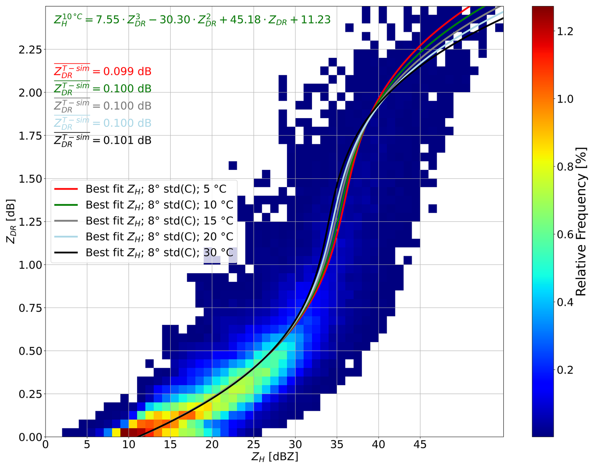
Figure 2 Z_H−Z_DR relationship based on T-matrix scattering simulations at 18° elevation angle and 10 °C using disdrometer measurements between November 2011 and December 2019 on the roof of the Institute for Geosciences, Department of Meteorology, University of Bonn, and 30 rain days between 2015 and 2017 from 68 Thies disdrometers of DWD (Chen et al., 2021). The best-fit lines of simulated Z_DR=f(Z_H) for different temperatures are indicated in different colors including the according inverted equation Z_H=f(Z_DR) (in green) achieved for 10 °C and std(C) of 8° used for Z_H calibration (see also Eq. 4). The mean values of Z_DR between 0 and 20 dBZ ($\stackrel{\mathrm{‾}}{Z_{\text{DR}}^{\text{T-sim}}}$) for the different temperatures are also given.

Only small differences in average simulated Z_DR in light rain ($\stackrel{\mathrm{‾}}{Z_{\text{DR}}^{\text{T-sim}}}$) and best-fit lines of Z_DR=f(Z_H) for different temperatures between 5 and 30 °C in Fig. 2 demonstrate that temperature dependencies can be neglected. Thus, $\stackrel{\mathrm{‾}}{Z_{\text{DR}}^{\text{T-sim}}}=\mathrm{0.1}$ dB is determined as the intrinsic Z_DR value in light rain for X-band radar data at elevation angles of 18°. The results are in agreement with those of Sanchez-Rivas and Rico-Ramirez (2022) (with an intrinsic Z_DR of 0.18 dB) and Zeyong et al. (2019) (with an intrinsic Z_DR in the range from 0.25–0.35 dB), despite slightly smaller values in comparison (most likely due to different radar configurations and varying climatic conditions).

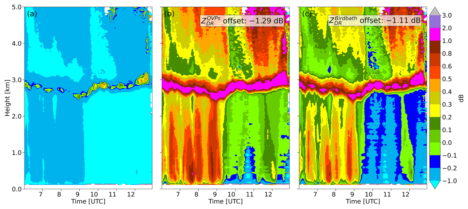
Figure 3 QVPs of Z_DR not offset corrected (a), offset corrected using QVP method (b) and birdbath scan method (c) for the 3 July 2013, from 06:00 to 13:00 UTC.

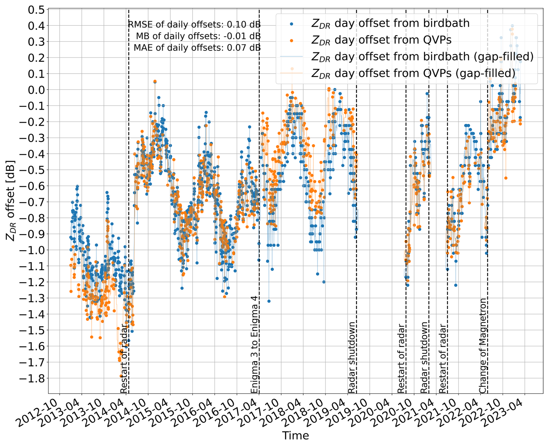
Figure 4 Daily Z_DR offsets calculated using for the period between January 2013–March 2023 the QVP (orange) and birdbath scan (blue) method, respectively. The times of important changes in BoXPol are given as vertical dashed lines with the respective caption. RMSE, MB and MAE calculated for the time period between 24 April 2014 and 3 April 2017 are shown as well.

Finally, the median of a day's $Z_{\text{DR}}^{\text{off}}$ values ($\text{med}\left[Z_{\text{DR}}^{\text{off}}\right]$) gives the daily Z_DR offset. Daily offsets are only calculated if the standard deviation of $Z_{\text{DR}}^{\text{off}}$ is <0.2 dB with at least >100 valid values. Days without defined offset are filled with a centered 30 d rolling mean of $\text{med}\left[Z_{\text{DR}}^{\text{off}}\right]$. Note, daily Z_DR offsets have to be subtracted from the measured Z_DR of the PPI scans.

Z_DR offsets derived from the birdbath scan calculated following Pejcic et al. (2022) but with a stricter filtering using only data between 20th and 80th percentile (instead of 10th and 90th percentile) are now compared with the ones obtained with the modified QVP method for the period from June 2014–April 2017. Therefore, the same gap-filling procedure as described above is applied to the birdbath scan Z_DR offset values. E.g., on 3 July 2013 the offset values obtained with the two methods show a relatively large difference of 0.18 dB (Fig. 3). Negative Z_DR values (between 0 and −0.1 dB) directly above the ML together with even more negative values of up to −1 dB in the liquid phase (panel (c)) indicate that the offset derived with the birdbath method is not adequate for the 18° scan.

The Z_DR offset time series obtained with the two methods for the time period from January 2013–March 2023 show similar trends, but deviations of about 0.2 dB or more occur in the period from 2013–April 2014 and from April 2017–June 2019 (Fig. 4). Another period of larger deviations is seen around December 2021–June 2022. Differences between the two methods are most likely associated with changes of the Magnetron (accompanied by receiving channel calibrations), the software change from Enigma 3 to Enigma 4 and general restarts of the radar after system failures. Within the stable period from 24 April 2014–3 April 2017, however, the Z_DR offsets of the two methods are very close to each other. This is confirmed by a root-mean-square error (RMSE) of 0.1 dB, a mean-absolute error (MAE) of 0.07 dB and the mean-bias³ (MB) of −0.01 dB (e.g. Von Storch and Zwiers, 2002).

3.2 Z_H calibration using the Z_H−Z_DR relationship

In the next step Z_H is calibrated exploiting the Z_H−Z_DR relationship (e.g. Ryzhkov and Zrnic, 2019) but with Z_DR as a predictor for Z_H on PPIs at 18° elevation angles. In the following the method will be referred to as the reverse Z_H−Z_DR method, since, to the authors' knowledge, it has so far only been used to calibrate Z_DR.

Again, mixed or solid phase hydrometers are excluded by focusing on data at least 250 m below the height of the 0 °C isotherm taken from the ERA5 data set. Unlike for the Z_DR calibration, PPIs instead of QVPs are used and are filtered with ρ_HV>0.99 and, as in the Z_DR calibration, with ϕ_DP<30°. Like for the Z_DR calibration at least 100 non-NaN values are required along the azimuth dimension to be taken into account. Additionally, at least two thirds of the valid Z_H bins of a PPI must show a valid Z_DR value. Only days with at least 10 PPIs per day, each with at least 100 valid values, are used for further calculation. Each PPI with a Spearman correlation coefficient corr_spear<0.4 is excluded from further calculations of the daily Z_H offset. Here, corr_spear is calculated based on the positive Z_H and Z_DR values and is used because of possible deviations from the Gaussian, non-linearities and reduced sensitivity to outliers compared to the Pearson correlation coefficient. Finally, the simulated Z_H−Z_DR dependency (Fig. 2) provides the expected Z_H ($Z_{\mathrm{H}}^{\text{ideal}}$) per day based on the Z_DR values of the filtered PPIs. More precisely, the best fit of simulated Z_H at 10 °C with std(C) equals 8° is used:

$$\begin{array}{}\text{(4)}& Z_{\mathrm{H}}^{\text{ideal}}=\mathrm{7.55}\cdot Z_{\text{DR}}^{\mathrm{3}}-\mathrm{30.30}\cdot Z_{\text{DR}}^{\mathrm{2}}+\mathrm{45.18}\cdot Z_{\text{DR}}+\mathrm{11.23}.\end{array}$$

As outlined before, variations with temperature are neglectable for Z_DR<2 dB (Fig. 2) and the temperature chosen is roughly the average annual temperature in Germany. Similarly, changing the std(C) in the range from 5–12 ° has only minor influence (Fig. 5). The expected $Z_{\mathrm{H}}^{\text{ideal}}$ is subtracted from the measured Z_H to obtain the calibration offset of a PPI ($Z_{\mathrm{H}}^{\text{off}}=Z_{\mathrm{H}}-Z_{\mathrm{H}}^{\text{ideal}}$). Again, only values between the 20th and 80th percentile of $Z_{\mathrm{H}}^{\text{off}}$ and with a standard deviation of $Z_{\mathrm{H}}^{\text{off}}<\mathrm{4}\mathrm{dB}$ are considered to derive the daily offset. These thresholds have been chosen based on rough visual impressions of the daily standard deviations of the GPM derived Z_H offsets in Pejcic et al. (2022), Louf and Protat (2023) and Protat et al. (2022) (their Figs. 2, 12 and 2, respectively).

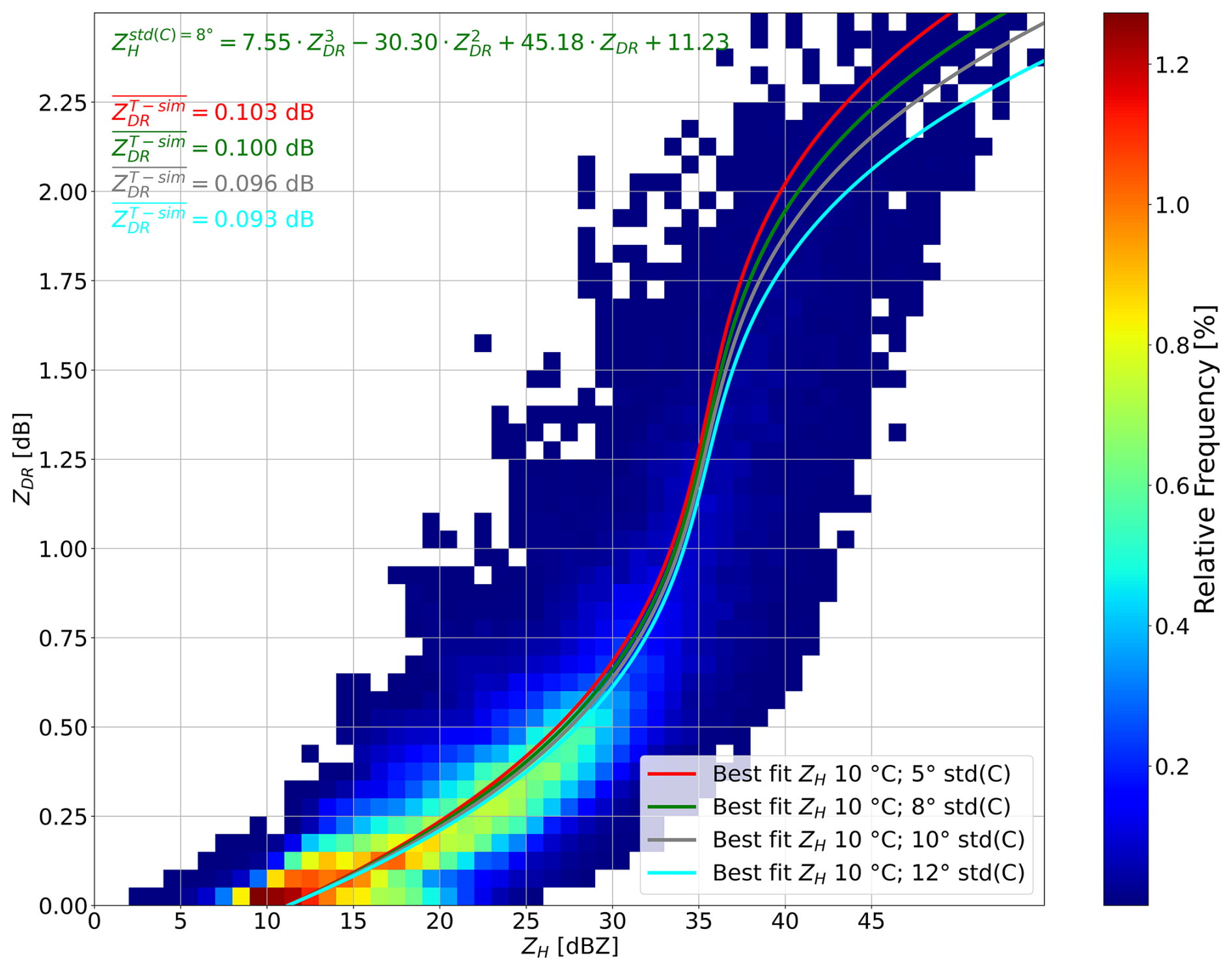
Figure 5 As in Fig. 2 but the best-fit lines of simulated Z_DR=f(Z_H) at a constant temperature of 10 °C with various std(C) and the mean values of Z_DR between 0 and 20 dBZ ($\stackrel{\mathrm{‾}}{Z_{\text{DR}}^{\text{T-sim}}}$) for different std(C) values.

Finally, calculating the median of these filtered $Z_{\mathrm{H}}^{\text{off}}$ ($\text{med}\left[Z_{\mathrm{H}}^{\text{off}}\right]$) gives the daily Z_H offset. Using the median instead of the mean reduces the impact of outliers caused by e.g. size sorting effects.

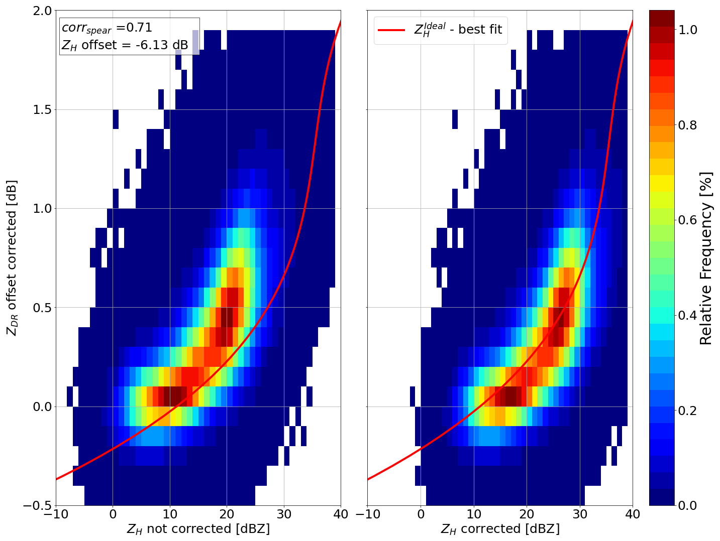
Figure 6 Two-dimensional histograms of offset-corrected Z_DR versus Z_H for 3 July 2013: (a) using uncorrected Z_H and (b) using offset-corrected Z_H, based on the reverse Z_H−Z_DR method. The thick red line represents the calculated ideal reflectivity ($Z_{\mathrm{H}}^{\text{ideal}}$), corresponding to the best fit obtained from Eq. (4).

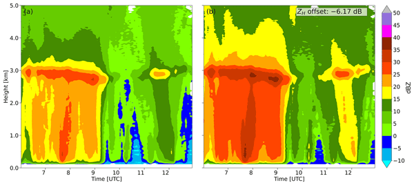
Consistent with the methodology for the calibration of Z_DR, any gaps in the time series of med [$Z_{\mathrm{H}}^{\text{off}}$] are filled using a rolling mean of 30 d. Offsets are defined to be subtracted from the measured Z_H values to obtain the offset-corrected Z_H. As an example, Fig. 6 demonstrates the performance of the method, i.e. the offset-corrected Z_H−Z_DR distribution is shifted towards the ideal simulated Z_H−Z_DR curve. QVPs of Z_H show the more pronounced bright band and aggregation signature (Figs. 3 and 7), whereby the higher values of Z_H after offset correction appear to be more realistic.

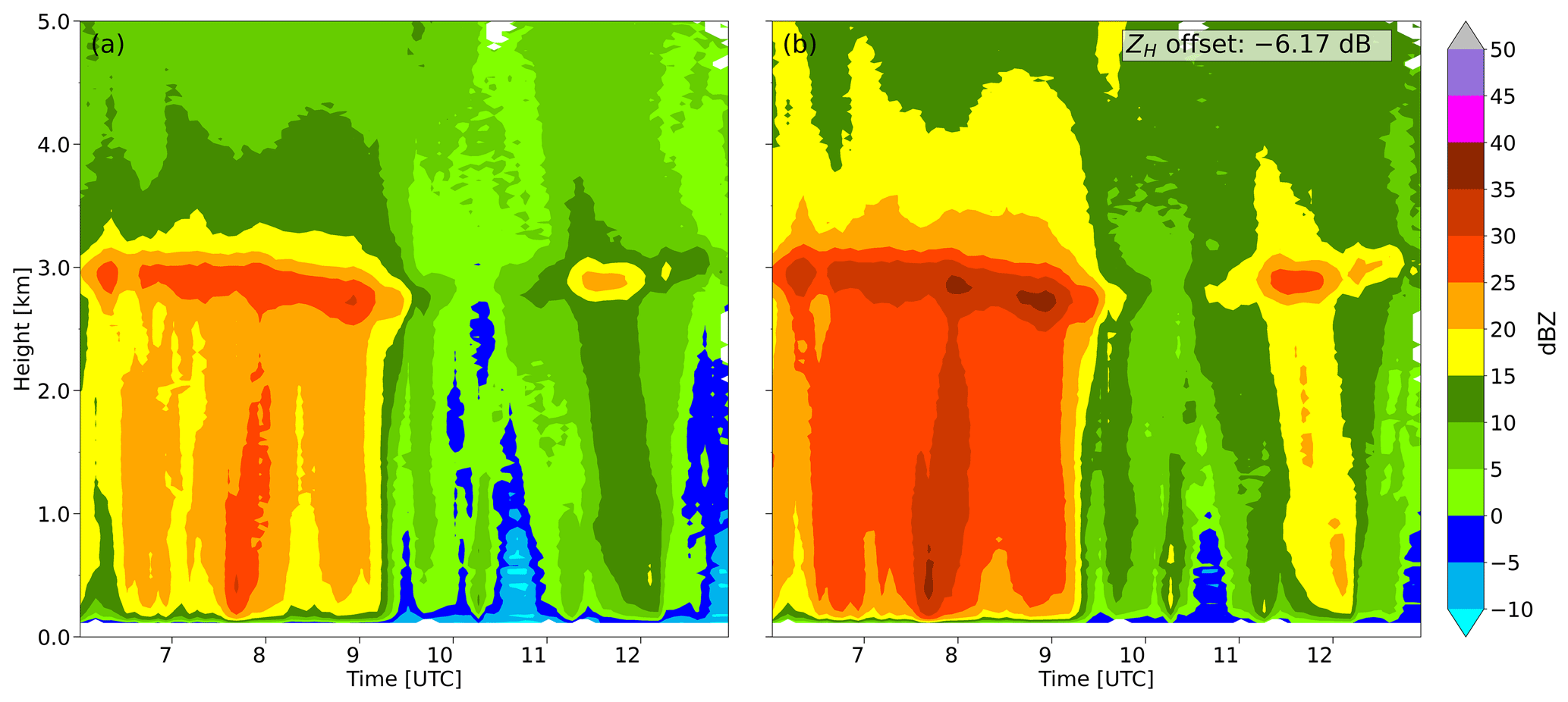
Figure 7 QVPs of (a) uncorrected and (b) corrected Z_H using the reverse Z_H−Z_DR method for the 3 July 2013, from 06:00 UTC to 13:00 UTC.

3.2.1 Validation of Z_H-calibration using the self-consistency relationship

The relationship between the ratio $K_{\text{DP}}{Z}_{\mathrm{h}}^{-\mathrm{1}}$, with the reflectivity factor in linear scale ($Z_{\mathrm{h}}={\mathrm{10}}^{\mathrm{0.1}{Z}_{\mathrm{H}}}$) in mm⁶ m⁻³, and Z_DR in rain (e.g. Gorgucci et al., 2006) represents an alternative opportunity to calibrate radars (e.g. Marks et al., 2011). This technique is often utilized to calibrate Z_H of operational radars because, similar to the Z_H−Z_DR relationship, it does not require comparative analysis, e.g. with other technical devices or instruments (Lee et al., 2021). However, applying published self-consistency relationships derived in different geographical locations and climate regimes can lead to large discrepancies (Louf et al., 2019).

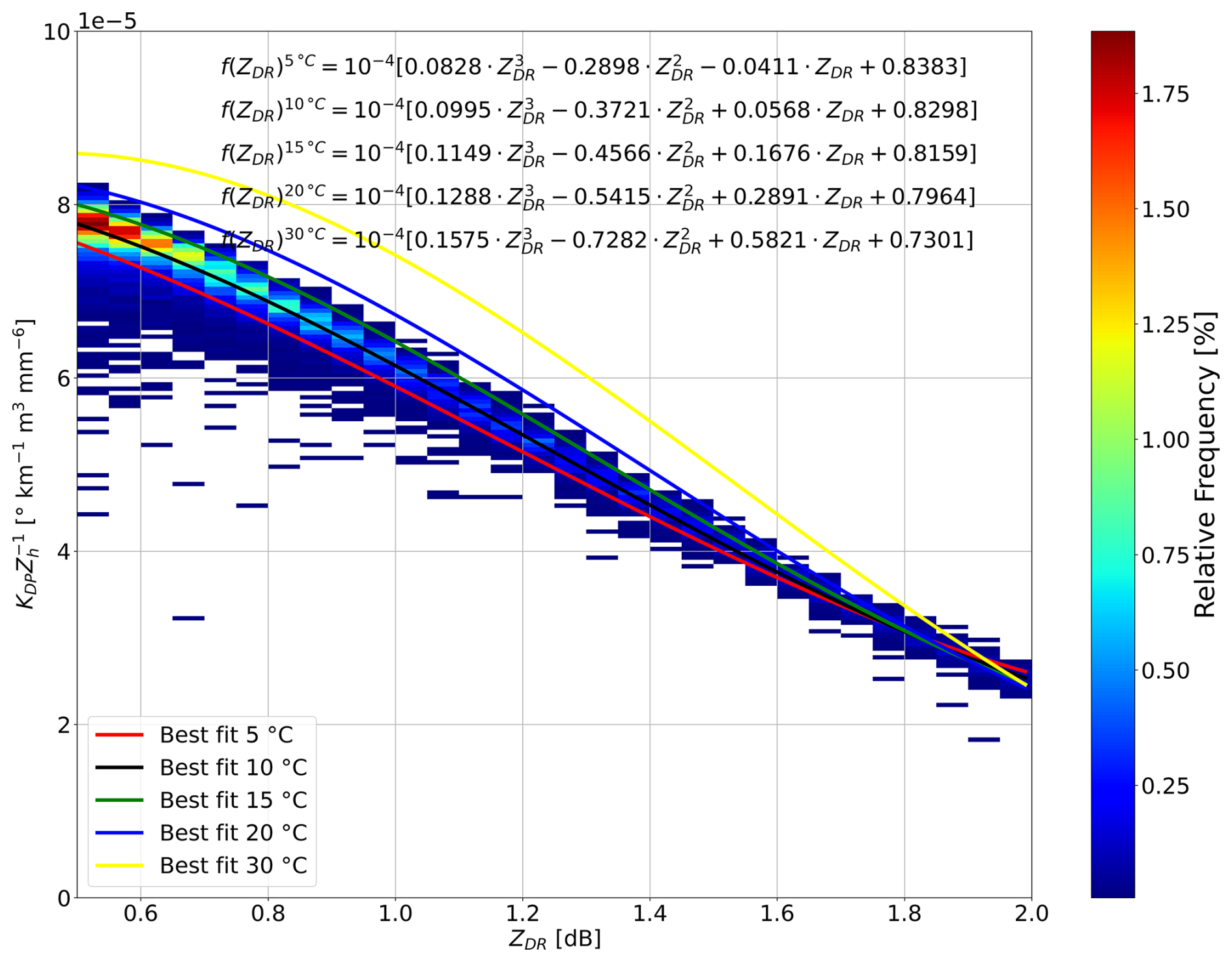
Figure 8 T-matrix simulated ($K_{\text{DP}}{Z}_{\mathrm{h}}^{-\mathrm{1}}$)-Z_DR dependencies at 18° elevation angle and 10 °C based on disdrometer measurements for the period from November 2011–December 2019 on the rooftop of the Institute of Geosciences, Section Meteorology, University of Bonn, and 30 rainy days between 2015 and 2017 from 68 Thies disdrometers of the DWD (Chen et al., 2021). The best fit lines of the simulated f(Z_DR) for different temperatures are also given.

Since the ratio $K_{\text{DP}}{Z}_{\mathrm{h}}^{-\mathrm{1}}$ is also temperature dependent at X-band (Ryzhkov and Zrnic, 2019), we derive a set of self-consistency relationships for Germany at various temperatures based on T-matrix simulated K_DP, Z_h and Z_DR using again the DSD dataset and the assumptions outlined in Sect. 3. Only DSDs with $\mathrm{0.5}\mathrm{dB}>Z_{\text{DR}}<\mathrm{2}\mathrm{dB}$ (Louf et al., 2019) are considered to determine the resulting best-fit equations f(Z_DR) for the ratio $K_{\text{DP}}{Z}_{\mathrm{h}}^{-\mathrm{1}}$ as presented in Fig. 8. Subsequently we determine the expected Z_H, in the following referred to as $Z_{\mathrm{H}}^{\text{self}}$, for comparison with the offset corrected Z_H using the reverse Z_H−Z_DR method, with the following equation:

$$\begin{array}{}\text{(5)}& Z_{\mathrm{H}}^{\text{self}}\left(i\right)=\mathrm{10}{\log }_{\mathrm{10}}\left({\displaystyle \frac{K_{\text{DP}}\left(i\right)}{f\left(Z_{\text{DR}}\right)\left(i\right)}}\right),\end{array}$$

where the index i indicates the different equations for 5, 10, 15, 20 and 30 °C, respectively. For a comparison in nearly homogeneous conditions, QVPs of stratiform rain events are generated, whereby in contrast to Sect. 3.1, prior filtering combines the use of the ML detection algorithm by Wolfensberger et al. (2016) but modified for application to QVPs by Trömel et al. (2019) and the Shannon information entropy (see Appendix A, Trömel et al., 2023). Filtering with the minimum Shannon information entropy min(η(X)_norm)≥0.85 guarantees an increased degree of homogeneity in the PPI scans prior QVP generation. All QVP bins derived with the PPIs at 18° elevation monitored between 2013 and 2023 fulfilling these criteria are considered. The validation based on temperature information obtained from ERA5 further demonstrates the suitability of the stratiform filter technique (in particular the ML detection algorithm, see Appendix B). As above, following Louf et al. (2019) and Ryzhkov and Zrnic (2019), filtering with $\mathrm{0.5}\mathrm{dB}<Z_{\text{DR}}<\mathrm{2}\mathrm{dB}$, SNR>25 dB, ρ_HV>0.99 and additionally ϕ_DP<30° is applied to the QVPs (see Sect. 3.1). Here, K_DP and offset-corrected Z_DR values of these QVPs are used to calculate $Z_{\mathrm{H}}^{\text{self}}$ using Eq. (5) and opposed to the offset-corrected Z_H of the QVPs. The comparison shows a moderate agreement, as indicated by the correlation of 0.63 (Fig. 9). Additionally, the majority of $Z_{\mathrm{H}}^{\text{self}}$ values are larger than the measured Z_H, showing a MB⁴ of 2.15 dB. The RMSE of 3.76 dB and the MAE of 3.08 dB confirm this observation.

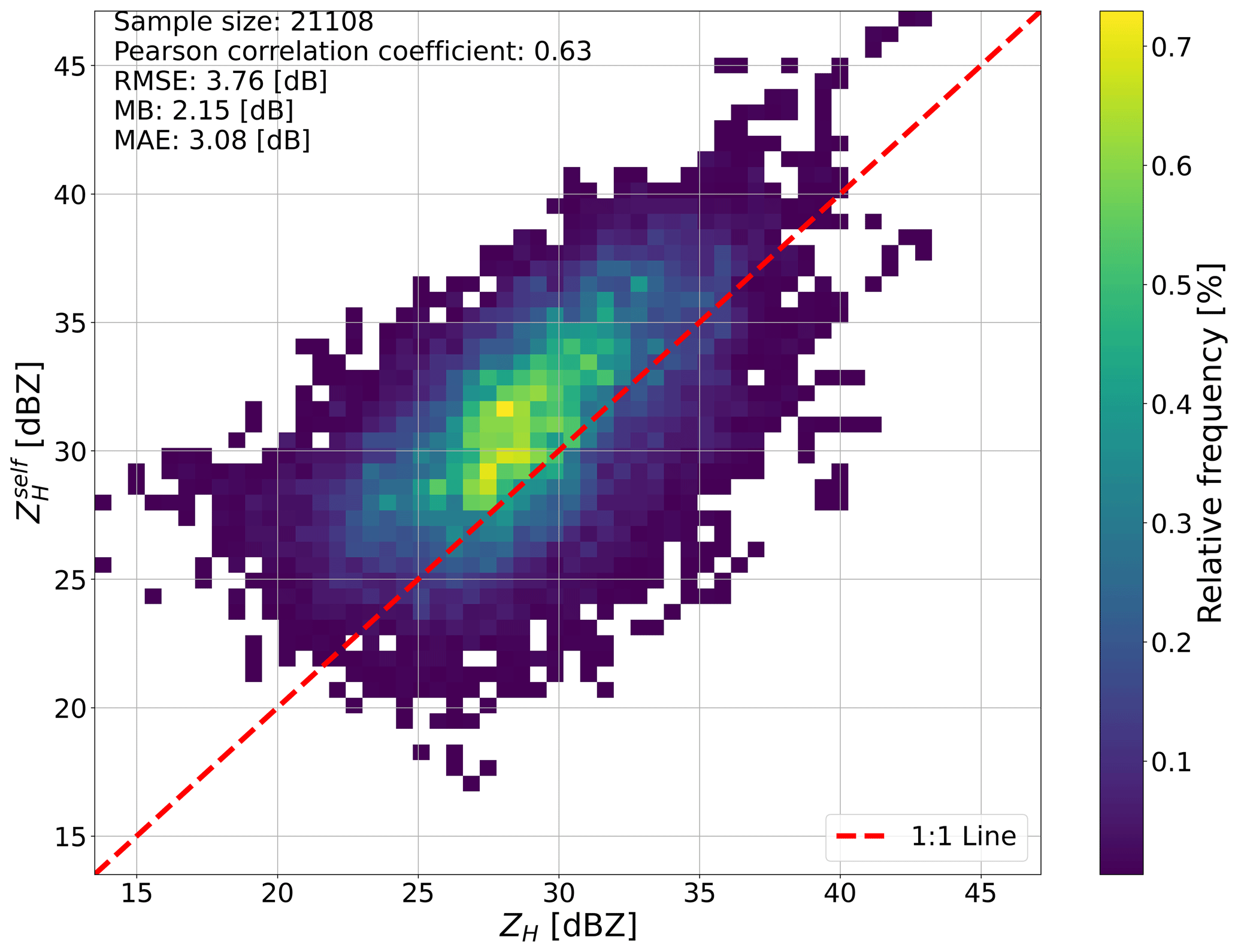
Figure 9 2D histogram of $Z_{\mathrm{H}}^{\text{self}}$ (see Eq. 5) versus measured and offset corrected Z_H using the reverse Z_H−Z_DR method in the time period from 2013–2023. In addition to the sample size, Pearson correlation coefficient, RMSE, MB and MAE are also given.

Louf et al. (2019) show in their Fig. 15 the $Z_{\mathrm{H}}^{\text{self}}$ against calibrated Z_H obtained from the C-band polarimetric radar located near Darwin in northern Australia, using different raindrop shape models at 20 °C temperature and two different std(C). Overall, the distribution shown in Fig. 9 compares well with Fig. 15 in Louf et al. (2019), giving additional confidence also in using the 30 d rolling mean gap-filling procedure of the Z_H offsets. However, Fig. 9 shows higher values of $Z_{\mathrm{H}}^{\text{self}}$ and more outliers. Intrinsic uncertainties associated with the K_DP processing on the one hand, the temperature dependency, assumptions about the canting angle distribution and the chosen raindrop shape model in the T-matrix simulations on the other hand, may affect the results.

To gain more insight using self consistency Z_H calibration we additionally calculate Z_H offsets on a daily basis in a similar way as the Z_DR offsets (Sect. 3.1). In the following section, the two different Z_H offset calibration techniques are compared with each other and validated using satellite information.

3.2.2 Validation of Z_H-calibration using satellite information

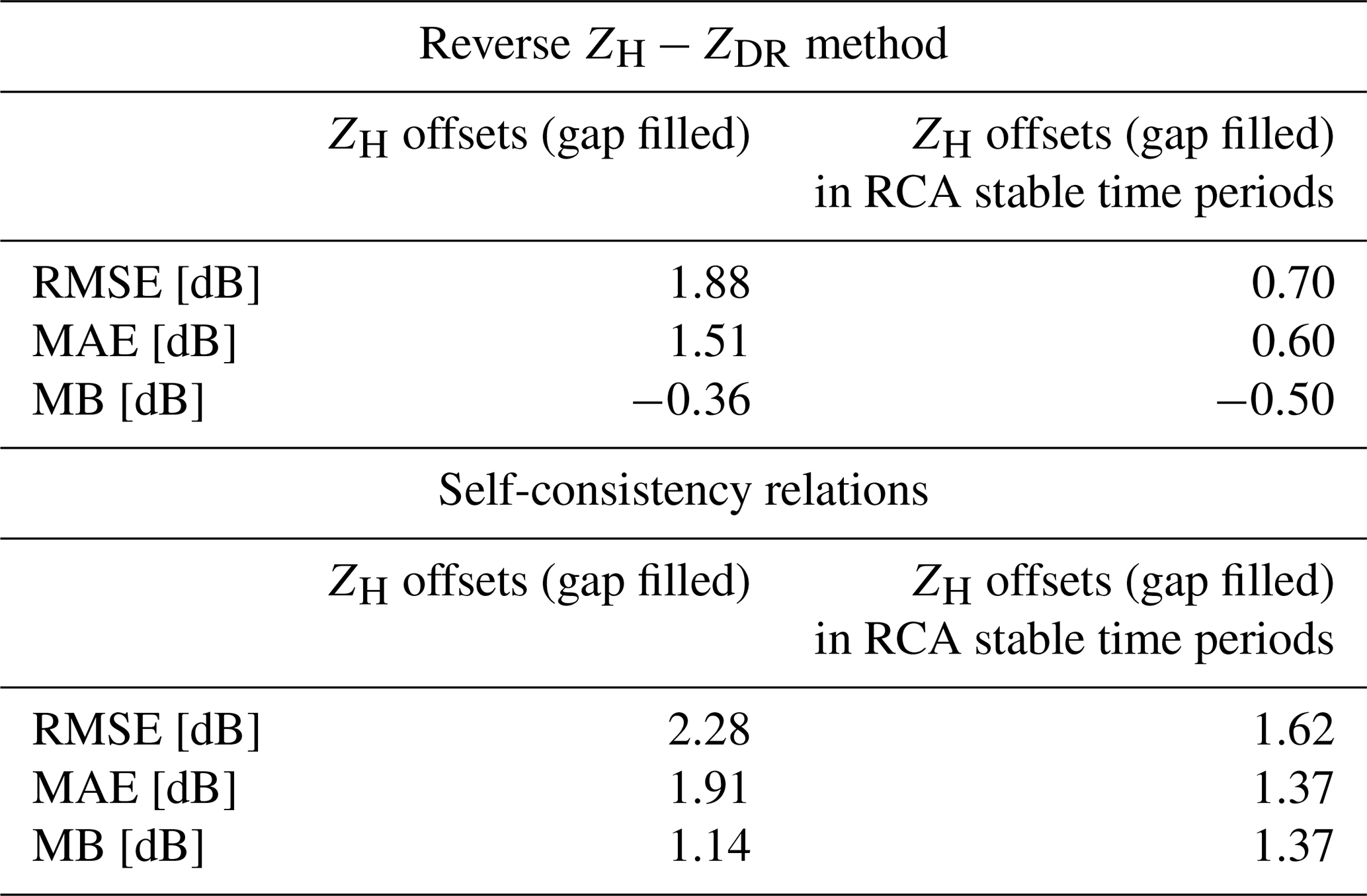
Satellite measurements of the Dual-frequency Precipitation Radar (DPR) operating on the Global Precipitation Mission (GPM; e.g. Hou et al., 2014; Pejcic et al., 2020) core satellite, as well as its predecessor the Tropical Rainfall Measurement Mission (TRMM; see e.g. Kozu et al., 2001; Joss et al., 2006) have been demonstrated to be a valuable data source for the calibration of ground based Z_H radar measurements (e.g., Pejcic et al., 2022; Louf and Protat, 2023; Louf et al., 2019; Warren et al., 2018; Loulli et al., 2025; Anagnostou et al., 2001). Thus, Z_H offsets obtained in this study are compared with the ones calculated by Pejcic et al. (2022) in the period between 2014 and June 2019. Daily average Z_H offsets based on the differences between measurements of BoXPol and the satellite-based K_u-band radar (part of DPR, explained in more detail in Pejcic et al., 2022) are compared with daily offsets obtained using the reverse Z_H−Z_DR method and the self consistency relations (see Fig. 10). The reverse Z_H−Z_DR method provides 544 daily Z_H offsets, whereas the self-consistency method only provides 148. For the point-to-point comparison (nearest time of overflight and 30 d rolling mean gap filled Z_H offsets), both the RMSE of 1.88 dB and the MAE of 1.51 dB (MB⁵ $=-\mathrm{0.36}\mathrm{dB}$) are in an acceptable range but relatively high. The differing sample sizes (92 overflights of GPM), may explain part of the deviations. At the same time, however, this comparison demonstrates the applicability of the 30 d rolling mean to obtain a gap-filled time series of Z_H offsets. And even though the DPR itself has a calibration accuracy of less than ±1 dB (Masaki et al., 2020; Warren et al., 2018), intrinsic uncertainties of $\approx \mathrm{0.25}-\mathrm{0.5}\mathrm{dB}$ for the K_u channel of the DPR must be considered in interpreting the accuracy of the reverse Z_H−Z_DR method (see for example Figs. 8 and 9 in Masaki et al., 2020). Furthermore, Pejcic et al. (2022) uses the mean value instead of the median for the respective days, which gives outliers more weight, potentially increasing the discrepancies between GPM derived Z_H offsets and med[$Z_{\mathrm{H}}^{\text{off}}$]. RMSE and MAE improve only slightly without the 30 d rolling mean gap filled procedure (not shown). For the 30 d rolling mean gap filled Z_H offsets obtained from self-consistency relations, both the RMSE (2.23 dB) and the MAE (1.87 dB) are larger and offsets are more negatively biased compared to results obtained with the reverse Z_H−Z_DR method. The variabilities over the days, however, are rather similar for all three methods.

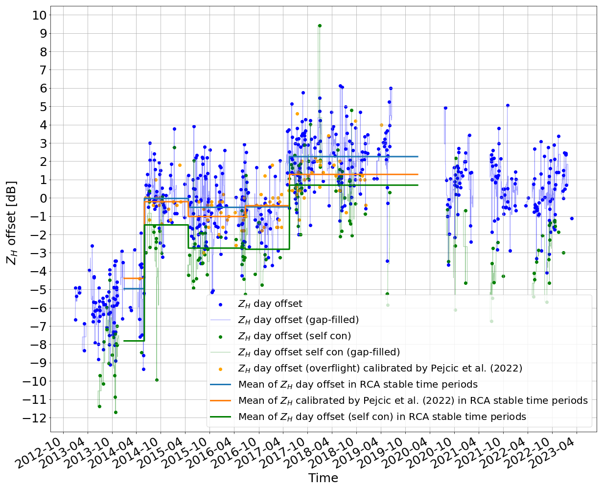
Figure 10 Daily Z_H offsets obtained from the reverse Z_H−Z_DR method (blue dots), the GPM overflights (orange dots; Pejcic et al., 2022) and the self-consistency relations (Δ_self[Z_H]) in the period between January 2013–March 2023, respectively. Mean values of Z_H offsets in RCA stable time periods from Pejcic et al. (2022) are given as blue, orange and green horizontal lines, respectively.

Additionally, the averaged satellite-derived Z_H offsets in stable calibration time periods identified with the relative calibration adjustment (RCA) technique (see Pejcic et al., 2022, for more information) are compared with according averaged values based on the 30 d rolling mean gap-filled Z_H offsets obtained from the reverse Z_H−Z_DR method and from the self-consistency relations (Fig. 8). The averaging of the offsets obtained from satellite information over this stable time periods reduces the uncertainties of the GPM derived offsets to less than 1 dB (e.g. Louf and Protat, 2023; Protat et al., 2022). Seasonal Variations triggered by e.g. changing vegetation (Louf and Protat, 2023) challenge the RCA method to identify stable time periods. Seasonal fluctuations are also recognizable in Pejcic et al. (2022) (their Fig. 2) and may have impacted the accuracy of the averaged Z_H offset value obtained from GPM overpasses in RCA stable time periods. Especially the stronger deviations between the averaged 30 d rolling mean gap filled Z_H offsets obtained by using the reverse Z_H−Z_DR method and the ones from the GPM overpasses in the last time period (19 May 2017–30 June 2019) are likely associated with these seasonal fluctuations. Nevertheless, both smaller RMSE and MAE strengthen confidence in using the reverse Z_H−Z_DR method instead of the self-consistency relations (Table 3). In summary, since the self-consistency method bears several uncertainties, as well as a smaller sample size compared to the reverse Z_H−Z_DR method (148 versus 544 valid days) and more confidence can be assigned to the comparison with satellite overflights, we conclude on the overall reliability of the reverse Z_H−Z_DR method for Z_H calibration.

4 Summary, discussion and outlook

The birdbath method, broadly used for Z_DR calibration, provided only for a limited time period (April 2014–April 2017) of the BoXPol data set reliable results. Otherwise, inaccuracies of more than 0.2 dB have been detected. Instead, the approach by Sanchez-Rivas and Rico-Ramirez (2022) has been modified and applied successfully to ensure sufficient accuracy of Z_DR for the entire period (2013–2023).

This study aims to raise awareness of the need to critically use the birdbath method (or any other method based on one elevation scan only) and not apply the resulting offsets to the entire volume scan without further verification. Elevation dependent offsets have been identified already for other radars as well (e.g. Blanke et al., 2025). It may be necessary to calculate an individual Z_DR offset value for each of the elevations of interest, which can be time consuming and computationally expensive.

Since accurately calibrated Z_DR values are key for applications such as QPE, HMC, or Z_H calibration exploiting the reverse Z_H−Z_DR method, further research is required to ensure reliable quantitative use of Z_DR in radar meteorology.

Table 3 RMSE, MAE and MB for the 30 d rolling mean gap-filled Z_H offsets obtained using the reverse Z_H−Z_DR method and the self-consistency relations in comparison with GPM overflights (both also for the mean values in RCA stable time periods), as presented in Fig. 10.

The reverse Z_H−Z_DR method has been validated and compared with satellite-based measurements and self-consistency relations. Z_H offsets derived with the reverse Z_H−Z_DR methodology agree well with the averaged Z_H offsets derived from GPM overpasses in stable RCA periods between 2014 and 2019 (Pejcic et al., 2022). Even a direct point-to-point comparison of daily Z_H offsets, which is critical due to the large difference in sample sizes, shows similar trends and acceptable RMSE and MAE values. To gain additional insights, expected Z_H values using self-consistency relations ($Z_{\mathrm{H}}^{\text{self}}$) based on QVPs have been calculated as well. A stratiform filtering technique (see Trömel et al., 2023 and Appendix A) guarantees a sufficient degree of homogeneity for QVP generation. The comparison of $Z_{\mathrm{H}}^{\text{self}}$ and Z_H calibrated with the reverse Z_H−Z_DR method are consistent with results shown in Louf et al. (2019), with acceptable values for the RMSE, MAE and MB. In addition, the general overestimation of $Z_{\mathrm{H}}^{\text{self}}$ values is in agreement with the more negative daily derived Z_H offset values using self-consistency relations compared to the ones using the reverse Z_H−Z_DR method. The small number of outliers in $Z_{\mathrm{H}}^{\text{self}}$ can most likely be explained by uncertainties in K_DP derivations, DSD variability, temperature dependencies, assumptions on the canting angle distribution and the raindrop shape model used in the T-matrix simulations.

The comparison between $Z_{\mathrm{H}}^{\text{self}}$ and the offset corrected Z_H using the reverse Z_H−Z_DR method gives confidence in the use of the 30 d rolling mean gap-filling procedure to adequately fill missing Z_H offset values.

In summary, we conclude on the overall reliability of the reverse Z_H−Z_DR method for Z_H calibration assuming a sufficiently accurate prior calibration of Z_DR. It may serve as a powerful alternative to standard Z_H calibration techniques like self-consistency relationships, and/or can be used, if satellite-based information for most accurate calibration of Z_H is missing. We do not intend to suggest that the self-consistency method is generally inferior. Rather, we wish to emphasize that BoXPols Z_H is calibrated with the method introduced with sufficient accuracy and, compared with an already established method, with even greater precision. Regarding satellite-based calibration, seasonal variations and their impact on RCA stable time periods (Pejcic et al., 2022) could be addressed in the future by applying a dynamic clutter map (Louf and Protat, 2023) to reduce potential uncertainties in the GPM derived Z_H offset values.

Even though diurnal variations have been partially observed in the Z_DR offsets, this study aimed at daily Z_DR and Z_H offsets, deleting days with higher variability in the offset values (Z_DR offset standard deviation>0.2 dB; Z_H offset standard deviation>4 dB). However, calculations of temporally higher resolved offsets could potentially lead to more accurate estimates of offsets and especially reduce potential errors associated with the gap-filling method based on a 30 d rolling mean. To enable also the inclusion of e.g. sequences not fulfilling the filtering criteria for light rain, or even more intense convective events in the offset calculations, other Z_H-calibration methods, e.g. the one proposed by Diederich et al. (2015) using A_H, or methods in the integrated Satellite and Clutter Absolute Radar calibration (SCAR; Louf et al., 2019; Louf and Protat, 2023) scheme like solar calibration could be combined with the introduced reverse Z_H−Z_DR method. Further validation of the reverse Z_H−Z_DR method in different climate regimes, at different radar wavelengths, and with an increased number of GPM overflights, should be carried out in the future.

Appendix A: Shannon information entropy and Melting Layer (ML) detection to identify homogeneous (stratiform) events

The QVP methodology requires nearly homogeneous weather conditions, such that the inherent averaging process results in a significant reduction of the statistical errors (Ryzhkov et al., 2016), quantified e.g. with the standard error of the mean (Von Storch and Zwiers, 2002). Additional variants of the QVP methodology, e.g. range-defined QVPs (RD-QVPs; Tobin and Kumjian, 2017) using all available elevation scans within an inverse distance weighting procedure, or columnar vertical profiles (CVPs; Murphy et al., 2020) also using multiple elevation scans but in limited range and azimuth sectors, have been developed for different applications. However, the required degree of homogeneity or acceptable inhomogeneities, caused e.g. by embedded convection or nonuniform beam filling (NBF; e.g. Ryzhkov, 2007; Ryzhkov and Zrnic, 2019, especially for higher antenna beamwidths), has not yet been explored for these methodologies to the authors' knowledge. Instead, rather subjective “by eye” impressions are mostly used.

In order to distinguish between homogeneous (stratiform) and convective events or exclude embedded convection from widespread stratiform rain, an automated and robust method is introduced. It combines ML detection with the Shannon information entropy (η(X); Shannon, 1948; Trömel et al., 2023). The latter measures the average degree of uncertainty of the realisations of a random variable. For the sake of simplicity, a normalised version is used. Given a discrete random variable (X) with possible realisations $x_{\mathrm{1}},\mathrm{\dots },x_m$ and probabilities $\mathrm{P}\left(x_{\mathrm{1}}\right),\mathrm{\dots },\mathrm{P}\left(x_m\right)$, the normalised Shannon information entropy (η(X)_norm) of X is defined as

$$\begin{array}{}\text{(A1)}& \begin{array}{rl}\mathit{\eta }(X{)}_{\text{norm}}& ={\displaystyle \frac{\mathit{\eta }\left(X\right)}{\mathit{\eta }(X{)}_{\text{max}}}}\\ & =-{\displaystyle \frac{\mathrm{1}}{{\log }_{\mathrm{10}}\left(m\right)}}\sum _{k=\mathrm{1}}^m\mathrm{P}\left(x_k\right){\log }_{\mathrm{10}}\left(\mathrm{P}\right(x_k\left)\right)\\ & ={\displaystyle \frac{\mathrm{1}}{{\log }_{\mathrm{10}}\left(m\right)}}\sum _{k=\mathrm{1}}^n\mathrm{P}\left(x_k\right)I\left(x_k\right).\end{array}\end{array}$$

In Eq. (A1) the maximum possible Shannon information entropy (η(X)_max) follows a uniform distribution with sample size m and $\mathrm{P}\left(x_k\right)=\mathrm{1}/m$ with $k=\mathrm{1},\mathrm{\dots },m$. I(x_k) denotes the so-called self information (e.g. Borda, 2011) of individual realisations x_k of X and quantifies the level of “surprise” of a specific event. The higher (smaller) the probability of an event, the less (more) “surprising” it is and therefore I(x_k) is smaller (larger). The probabilities are non-negative (P(x_k)≥0) and additive (${\sum }_{k=\mathrm{1}}^m\mathrm{P}\left(x_k\right)=\mathrm{1}$; e.g. Han and Kobayashi, 2002). Thus, η(X) represents the expected value of the information content of X (η(X)=E[I(X)]; e.g. Borda, 2011).

In order to apply Eq. (A1) to PPI scans, the P(x_k) are calculated at each distance (range) over all azimuths, i.e. for a 1° beam width $\mathrm{P}\left(x_k\right)=x_k/{\sum }_{k=\mathrm{1}}^{\mathrm{360}}{x}_k$. In this study, the values x_k refer to either Z_H in linear scale ($Z_{\mathrm{h}}={\mathrm{10}}^{\mathrm{0.1}{Z}_{\mathrm{H}}}$), Z_DR in linear scale ($Z_{\text{dr}}={\mathrm{10}}^{\mathrm{0.1}{Z}_{\text{DR}}}$) (unitless), K_DP or ρ_HV at a certain range at azimuth k. Since Eq. (A1) is only defined for positive values, also K_DP is limited to values $>\mathrm{0}\mathrm{°}{\mathrm{km}}^{-\mathrm{1}}$.

Values of η(X)_norm close to 1 represent homogeneous conditions while values close to 0 represent inhomogeneous conditions. In this study a threshold of 0.85 is used to identify sufficiently homogeneous stratiform PPIs. The impact of embedded, more convective sectors on η(X)_norm within an overall stratiform event is illustrated in Fig. A1.

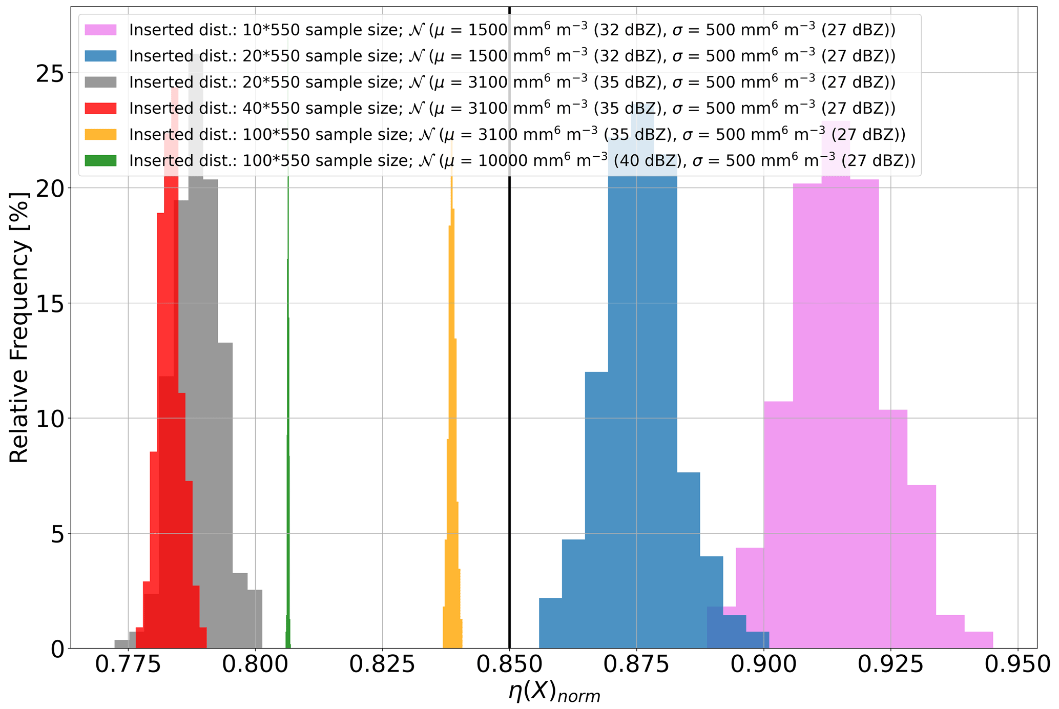
Figure A1 Z_h values of a fictitious PPI scan with 360 azimuths times 550 range bins in stratiform rain are described as a realization of a Gaussian distribution with a mean value of 100 mm⁶ m⁻³ and a standard deviation of 10 mm⁶ m⁻³ (𝒩 ($\mathit{\mu }=\mathrm{100}{\mathrm{mm}}^{\mathrm{6}}{\mathrm{m}}^{-\mathrm{3}}$ (20 dBZ), $\mathit{\sigma }=\mathrm{10}{\mathrm{mm}}^{\mathrm{6}}{\mathrm{m}}^{-\mathrm{3}}$ (10 dBZ))). Embedded convection is introduced by replacing for a certain number of azimuths (e.g., 20, 40, and 100 out of 360) at each distance stratiform Z_h values by the ones generated as a realization of a Gaussian distribution with increased μ values (e.g., 3100 mm⁶ m⁻³) and constant values of σ of 500 mm⁶ m⁻³. For illustration η(X)_norm is calculated based on these simulated Z_h values only and for different scenarios of embedded convection using Eq. (A1). Resulting distributions of η(X)_norm are shown in violet, blue, grey, red, yellow, and green if embedded convection is introduced with sample size 10×550 following 𝒩 ($\mathit{\mu }=\mathrm{1500}{\mathrm{mm}}^{\mathrm{6}}{\mathrm{m}}^{-\mathrm{3}}$ (32 dBZ), $\mathit{\sigma }=\mathrm{500}{\mathrm{mm}}^{\mathrm{6}}{\mathrm{m}}^{-\mathrm{3}}$ (27 dBZ)), with sample size 20×550 following 𝒩 ($\mathit{\mu }=\mathrm{1500}{\mathrm{mm}}^{\mathrm{6}}{\mathrm{m}}^{-\mathrm{3}}$ (32 dBZ), $\mathit{\sigma }=\mathrm{500}{\mathrm{mm}}^{\mathrm{6}}{\mathrm{m}}^{-\mathrm{3}}$ (27 dBZ)), with sample size 20×550 following 𝒩 ($\mathit{\mu }=\mathrm{3100}{\mathrm{mm}}^{\mathrm{6}}{\mathrm{m}}^{-\mathrm{3}}$ (35 dBZ), $\mathit{\sigma }=\mathrm{500}{\mathrm{mm}}^{\mathrm{6}}{\mathrm{m}}^{-\mathrm{3}}$ (27 dBZ)), with sample size 40×550 following 𝒩 ($\mathit{\mu }=\mathrm{3100}{\mathrm{mm}}^{\mathrm{6}}{\mathrm{m}}^{-\mathrm{3}}$ (35 dBZ), $\mathit{\sigma }=\mathrm{500}{\mathrm{mm}}^{\mathrm{6}}{\mathrm{m}}^{-\mathrm{3}}$ (27 dBZ)), with sample size 100×550 following 𝒩 ($\mathit{\mu }=\mathrm{3100}{\mathrm{mm}}^{\mathrm{6}}{\mathrm{m}}^{-\mathrm{3}}$ (35 dBZ), $\mathit{\sigma }=\mathrm{500}{\mathrm{mm}}^{\mathrm{6}}{\mathrm{m}}^{-\mathrm{3}}$ (27 dBZ)), and with sample size 100×550 following 𝒩 ($\mathit{\mu }=\mathrm{10}\mathrm{000}{\mathrm{mm}}^{\mathrm{6}}{\mathrm{m}}^{-\mathrm{3}}$ (40 dBZ), $\mathit{\sigma }=\mathrm{500}{\mathrm{mm}}^{\mathrm{6}}{\mathrm{m}}^{-\mathrm{3}}$ (27 dBZ)), respectively. The black line shows the used threshold in this study series of 0.85 for η(X)_norm.

As expected, η(X)_norm decreases with increasing μ of 𝒩(μ,σ) describing the embedded convection, but also the amount of inserted convective bins has a strong influence. First, η(X)_norm decreases with increasing number of convective bins (see violet versus blue distribution and grey versus red distribution in Fig. A1), however, if the sample size of convective pixels exceeds a certain fraction of the overall PPI, η(X)_norm increases again (see yellow distribution) but the PPI is still characterized as inhomogeneous (η(X)_norm<0.85). For even higher μ (10 000 mm⁶ m⁻³; green distribution) η(X)_norm is decreasing again. Note that the width of the η(X)_norm distributions narrows with increasing μ of the convective 𝒩(μ,σ) distribution and also with the number of inserted convective bins. This can be attributed to the constant and quite small $\mathit{\sigma }=\mathrm{500}{\mathrm{mm}}^{\mathrm{6}}{\mathrm{m}}^{-\mathrm{3}}$.

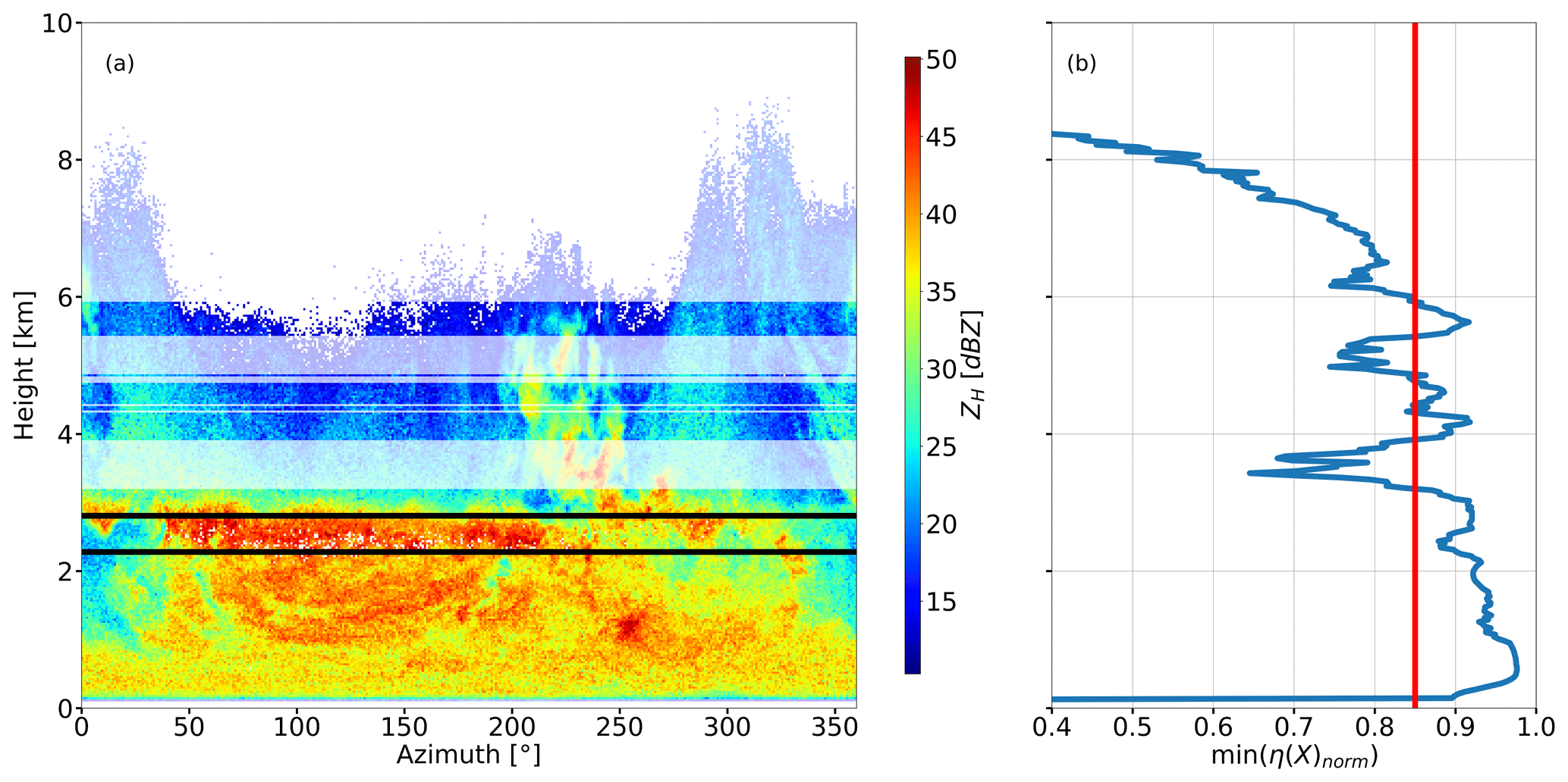
Figure A2 PPI of Z_H in an azimuth-height display (a) monitored with the polarimetric X-band radar in Bonn, BoXPol, on 30 May 2016 at 03:11 UTC. ML top and bottom heights are indicated as black lines and excluded inhomogenous sequences are displayed as transparent regions. The according profile of the minimum normalised Shannon information entropy (min(η(X)_norm)) (b) is shown together the applied threshold for filtering (0.85) as red line.

The overall recommended strategy combining ML detection and the Shannon information entropy to identify homogeneous stratiform events is as follows:

1. The ML detection of Wolfensberger et al. (2016) adapted to the QVP methodology (Ryzhkov et al., 2016; Trömel et al., 2014) is applied including the estimation of an average K_DP within the ML following Trömel et al. (2019) and removal of contributions of backscatter differential phase (δ). No (differential) attenuation correction is applied to the PPIs measured at 18° elevation. Only PPIs with a detected ML are considered as stratiform and enter as candidates for potentially homogeneous PPIs the ensuing analysis steps.

2. Time steps with a detected ML bottom at higher altitudes than ML top are neglected as well as cases with unrealistic heights for the ML top (>10 km).

3. ML top and bottom identified in 2. are treated as first guess estimates and modified to nearby profile locations, where ρ_HV returns to values above 0.97 (Giangrande et al., 2008) for better comparability with previous ML statistics as e.g. Trömel et al. (2019).

4. η(X)_norm is calculated at each range/height over the azimuth dimension as a function of Z_h, Z_dr, ρ_HV and K_DP (without δ contaminations), respectively.

5. If all η(X)_norm values obtained for the polarimetric variables mentioned in 4. are greater than or equal 0.85, the respective range gates are classified as stratiform and included in the overall stratiform data set. The methodology introduced filters both strong convective inclusions and sequences with a low number of valid measurements, e.g. near the cloud top. Assuming always a full 360° circle in Eq. (A1) to determine η(X)_max, regions with only few valid measurements are automatically filtered out via the enhanced η(X)_max in the denominator of Eq. (A1). Note that min(η(X)_norm) is mainly dominated by changes in Z_h, but any anomalous values in K_DP, Z_dr or ρ_HV can be treated appropriately to obtain the best possible homogeneous (stratiform) data sequences.

6. Finally, using the temperature information from ERA5, heights of the ML top are only allowed at temperatures between −6 and 4 °C, while height levels of the ML bottom are restricted to temperatures between −2 and 8 °C.

Figure A2 illustrates the resulting reduction of min(η(X)_norm) below the 0.85 threshold due to embedded convection in a measured PPI. Inhomogeneities near the cloud top are filtered out as well. In summary, tests and simulations showed that the min(η(X)_norm) threshold of 0.85 used in this study still allows some weaker embedded convective bins within an overall stratiform event (see e.g. the violet and blue distributions in Fig. A1). Depending on requirements, a higher threshold value (e.g. 0.9) for more aggressive filtering, or a weaker threshold value (e.g. 0.8 as in Trömel et al., 2023) for more restrained filtering could be used.

The entropy method can also be applied to different sectors of a PPI or a moving min(η(X)_norm) with suitable window sizes over the azimuth dimension could be used to identify homoegenous sectors within a PPI, which may in total not show a sufficient degree of homogeneity. Within the RDQVP framework, the method suggested may also identify the most inhomogeneous elevation scans to adjust the threshold value used for the ranges in the inverse distance weighting procedure (for more information see Tobin and Kumjian, 2017).

Furthermore, the so-called permutation entropy (PE; Henry and Judge, 2019; Bandt and Pompe, 2002) could be implemented in future studies. As described above, η(X) is positive semidefinite and negative K_DP values can't be taken directly into account. Additionally, the typically smaller range of values of Z_dr, ρ_HV and K_DP compared to Z_h reduces the impact of the aforementioned variables on min(η(X)_norm). However, PE is based on relative frequencies of permutations of partitioned one-dimensional data (on time-series data as shown in Bandt and Pompe, 2002, or applied on radar data, e.g. Z_h values over the azimuth dimension). Thus, by calculating the minimum of the normalized version of PE (PE_norm; Henry and Judge, 2019), it is guaranteed that polarimetric variables covering a smaller range of values (see step 5 above, e.g., for ρ_HV) may influence the homogeneity estimate to the same extent as those covering a larger range of values.

Appendix B: Validation of the melting layer detection algorithm using ERA5

ML top heights are mostly located below the 0 °C isotherm (e.g. Song et al., 2021; Romatschke, 2021). One possible reason are values of relative humidity with respect to water (RH water) below 100 % favoring sublimation instead of melting (e.g. Heymsfield et al., 2021; Carlin and Ryzhkov, 2019). Thus, the ML top height rather indicates the height of the 0 °C wet-bulb temperature (see e.g. https://glossary.ametsoc.org/wiki/wet-bulb-temperature/, last access: 26 March 2026). Besides sublimative cooling, faster falling rimed particles with higher density and/or larger aggregates result in a sagging of the ML and typical polarimetric ML (bright band) signatures at lower height levels (e.g. Carlin, 2018; Kumjian et al., 2016; Xie et al., 2016).

In order to evaluate the ML detection algorithm, detected ML top heights are compared with both the heights closest to the 0 °C wet-bulb temperature isotherm and environmental temperature isotherm obtained from ERA5 by linearly interpolating from the nearest grid point to the location of BoXPol, as a 2D distribution (see Fig. B1). To ensure a thorough validation, no predefined temperature thresholds are applied (like in step 6 in Appendix A).

The comparison between both height levels indicates a very good agreement. Also, in terms of statistical quantities, the RMSE with 270.40 m, the MAE with 78.14 m, the MB⁶ with 171.14 m, and especially the Pearson correlation coefficient of 0.95 demonstrate the reliability of the algorithm. Also, for the environmental 0 °C temperature isotherm, the statistical quantities show only slightly higher values and in line with e.g. Song et al. (2021), their Fig. 6. Uncertainties may arise due to the interpolation process from the temporally coarser grid of ERA5 (1 h) and intrinsic uncertainties.

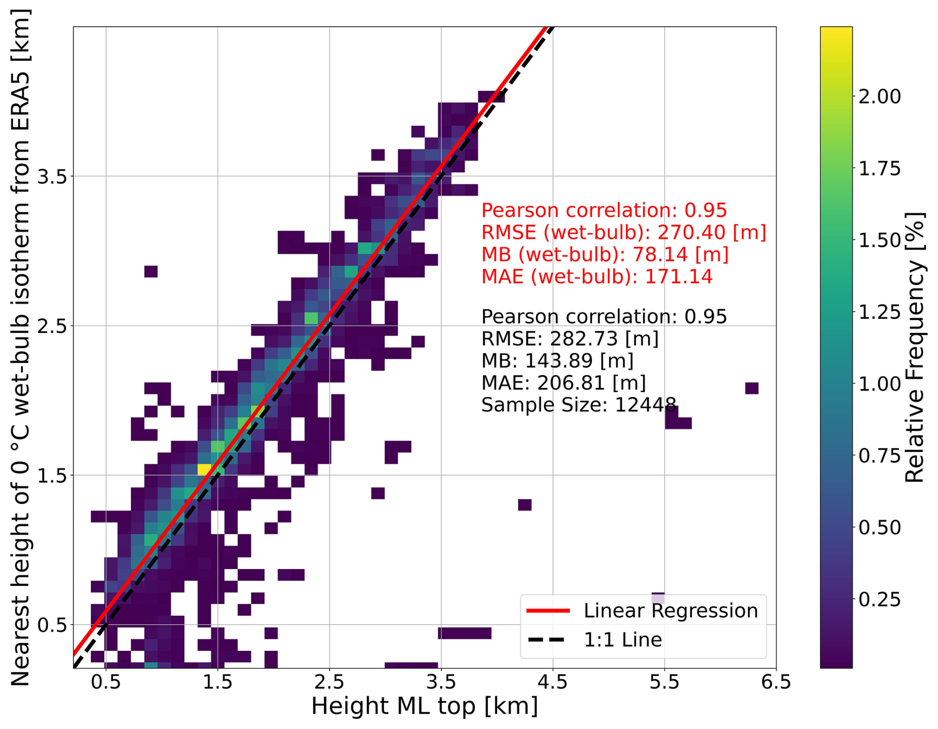
Figure B1 2D histogram of the 0 °C wet-bulb temperature height levels from ERA5 versus detected ML top heights. In addition, the Pearson correlation coefficient, RMSE, MB and MAE are given for the comparison of the ML top heights with both, the heights of the 0 °C wet-bulb temperature isotherm (red) and the 0 °C environmental temperature isotherm (black).