Towards harmonized measurements of condensable vapors: insights from the intercomparison of six chemical ionization mass spectrometers at a boreal forest site

Atmospheric new particle formation is driven by condensable vapors such as sulfuric acid and highly oxygenated organic molecules (HOMs). Measuring these gases is challenging because they are present at trace concentrations, they are easily lost through condensation onto surfaces, and they include a large number of chemically diverse species. Chemical Ionization Mass Spectrometry (CIMS) has been extensively used for their detection; however, results obtained in different studies are not always directly comparable. This limitation reflects differences in instrument designs, operating configurations, and reagent ion schemes employed. To investigate these factors, the Aerosol, Clouds and Trace Gases Research Infrastructure (ACTRIS) organized its first CIMS field intercomparison campaign (CI-FI1) during summer 2024 at a Finnish boreal forest site, the SMEAR II (Station for Measuring Forest Ecosystem-Atmosphere Relations) station. Six instruments employing different inlet designs, mass analyzers, and reagent ions were operated using their routine configurations and calibrated according to standard procedures. For sulfuric acid measured in nitrate mode, the conventional sulfuric acid calibration enabled moderately good agreement among instruments, although larger discrepancies were observed at the lower concentrations, typically observed during nighttime. When targeting higher-mass compounds, such as monoterpene-derived HOM monomers ($m/z$ 240–390) and dimers ($m/z$ 480–630), sulfuric acid calibration alone was insufficient to ensure measurement intercomparability and taking into consideration mass-dependent transmission differences proved important to achieve consistent results. Notably, good agreement was observed also for selected compounds measured in bromide mode by different instruments. Overall, the results demonstrate that comparable field measurements of condensable vapors by different CIMS instruments are achievable when all relevant calibration and correction factors are carefully considered. The results further highlight that similarities in instrument behavior are more closely associated with the inlet design and instrument operating conditions than with the reagent ion choice.

1 Introduction

The formation of new atmospheric aerosol particles is a complex process that has motivated extensive research efforts and promoted advances in analytical techniques. Although the species and mechanisms leading to the nucleation of aerosol particles vary with geographical location and elevation, studies indicate that new particle formation (NPF) involving multiple neutral compounds generally dominates over ion-induced pathways in the continental boundary layer (Kerminen et al., 2010; Zhao et al., 2024). Such neutral precursors of atmospheric aerosols are formed through the oxidation of volatile compounds, including sulfur dioxide (SO₂) and several volatile organic compounds (VOCs). SO₂ can be oxidized to sulfuric acid (H₂SO₄) by hydroxyl radicals (OH) or Criegee intermediates, whereas VOCs, such as monoterpenes, are oxidized by OH, ozone (O₃), or nitrate radicals (NO₃; Peräkylä et al., 2014), leading to the formation of highly oxygenated organic molecules (HOMs; Bianchi et al., 2019). H₂SO₄ and monoterpene-derived HOMs are among the species referred to as condensable vapors, which are low-volatility atmospheric gaseous compounds that act as direct aerosol precursors, and they have long been recognized as key contributors to the formation and growth of new atmospheric particles in the boreal forest (Ehn et al., 2014; Jokinen et al., 2012, 2015; Kulmala et al., 2013; Schobesberger et al., 2013). These neutral compounds are challenging to measure because (1) they are present at extremely low concentrations (often at parts-per-trillion to parts-per-quadrillion volume mixing ratios), (2) they readily condense onto surfaces due to their low volatility, and (3) they require charging before detection, which introduces additional complications, as different compounds may be charged and detected with different efficiencies. Adding to these challenges, (4) they comprise a large number of chemically diverse species: even when considering only the monoterpene-derived HOMs commonly targeted within this class, they cover a broad $m/z$ range and include molecules with varying numbers of carbon atoms and different functional groups and degrees of oxidation. Consequently, the detection of these NPF precursors requires analytical techniques that are both highly sensitive and capable of resolving a wide range of chemically diverse species.

From its early applications, chemical ionization mass spectrometry (CIMS) has proven to be particularly well suited for this purpose. Indeed, by selecting suitable reagent ions, it provides selective and sensitive online detection for a variety of chemical compounds. Commonly used reagent ions in atmospheric NPF studies include both negative and positive ions, such as nitrate (NO${}_{\mathrm{3}}^{-}$), acetate (CH₃COO⁻), bromide (Br⁻), and iodide (I⁻), as well as hydronium (H₃O⁺), ammonium (NH${}_{\mathrm{4}}^{+}$), nitrosonium (NO⁺), and protonated benzene cluster cations ((C₆H₆)${}_{\mathrm{2}}^{+}$). The selectivity of these and other reagent ions toward specific compounds has been investigated and reported in several studies (Zhang et al., 2023, 2024, and references therein).

Chemical ionization sampling has been performed both at reduced pressure and at ambient pressure. The first one offers comparatively better control over ionization conditions and is essentially unaffected by fluctuations in ambient parameters such as relative humidity (RH). The latter, on the other hand, substantially reduces analyte wall losses and provides a higher ionization probability compared to reduced pressure ionization methods, owing to the high collision rate between reagent ions and sample molecules at atmospheric pressure. It has therefore been more frequently employed for the detection of condensable vapors in situ.

Over the years, mass spectrometers with increasingly higher mass resolution have been developed, together with chemical ionization inlets designed to provide efficient sample ionization. Some inlet designs also allow operation with multiple reagent ion schemes, thereby expanding the range of target species that can be measured with a single mass spectrometer. In addition to the choice of reagent ion, other instrumental parameters can be tailored to the detection of targeted compounds. For example, by tuning the instrument voltages, the operator can alter the fragmentation and the transmission of clusters with different mass-to-charge ($m/z$) ratios within the mass spectrometer, thus affecting the sensitivity of the method (Lopez-Hilfiker et al., 2016; Wang et al., 2024).

The flexibility of CIMS, which makes it a powerful technique in atmospheric studies, also represents a challenge for data interpretation. Since these instruments are generally not calibrated for every targeted analyte, different setups and operating configurations, even when the same reagent ion is employed, can introduce substantial variability in quantitative measurement outcomes and complicate direct comparisons across studies. To date, however, the extent of these differences has not been comprehensively investigated or discussed. Furthermore, instrument-specific biases often remain unnoticed in standalone deployments. Intercomparison studies are therefore valuable tools for addressing these challenges, as they allow one to assess how well measurements from different instruments compare and, eventually, help identify methods toward more harmonized instrument performance. Such harmonization is needed to achieve consistent and robust measurements of condensable vapors and represents one of the objectives of the Centre for Reactive Trace Gases In Situ Measurements (CiGas) within the Aerosol, Clouds and Trace Gases Research Infrastructure (ACTRIS). In this framework, CiGas coordinates continuous long-term measurements of nitrogen oxides, non-methane hydrocarbons, oxygenated VOCs, and condensable vapors in the atmosphere, while also promoting intercomparison activities aimed at improving the consistency and comparability of measurements across different sites.

As part of these efforts, the present work provides insights from the first CIMS field intercomparison campaign organized by ACTRIS (ACTRIS CI-FI1), conducted over two weeks in summer 2024 at a Finnish boreal forest site, the SMEAR II (Station for Measuring Forest Ecosystem-Atmosphere Relations) station. During the intercomparison workshop, six instruments were operated using their routine configurations and settings, and calibrations were performed following standard procedures applied by each group. The objectives were to assess (a) how well measurements from different instruments, employing either the same or different reagent ions, compare under field conditions, and thus how effectively commonly used calibration approaches ensure inter-instrument comparability, and (b) to what extent factors other than reagent ion choice influence the instrument response toward selected compounds.

2 Methods

2.1 Measurement site and timeline

The ACTRIS CI-FI1 campaign took place between 26 July and 9 August 2024 at the SMEAR II station, located at the Hyytiälä Forestry Field Station of the University of Helsinki, in southern Finland (61°51^′ N, 24°17^′ E, 181 m above sea level). The measurement station is surrounded by a boreal coniferous forest characterized by managed pine stands and limited local pollution, primarily from two sawmills 5 km to the southeast and the city of Tampere 60 km to the southwest. The rationale and primary objectives of the SMEAR II station, originally established in 1982, have been thoroughly described by Hari and Kulmala (2005).

Table 1 Instruments participating in the ACTRIS CI-FI1 campaign. Details include institute affiliation, mass spectrometer type, chemical ionization inlet, and reagent ion.

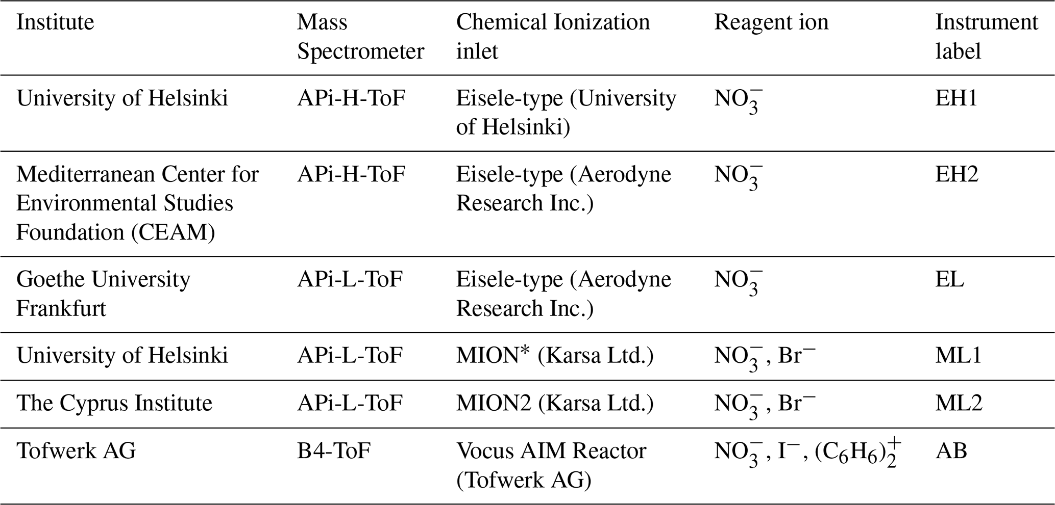
The present study involved multiple research teams and a total of six mass spectrometers (Table 1). Five of these were Atmospheric Pressure interface Time-of-Flight (APi-ToF, Tofwerk AG) mass spectrometers, including three long Time-of-Flight (L-ToF, mass resolution 6000–14 000 Th $/$ Th; 1 Th = 1 Da $/$ e, where e is the elementary charge) and two high-resolution Time-of-Flight (H-ToF, mass resolution 3000–7000 Th $/$ Th) mass spectrometers. Three out of the five APi-ToFs featured Eisele-type inlets (Eisele and Tanner, 1991, 1993; Jokinen et al., 2012) operated with NO${}_{\mathrm{3}}^{-}$ ions, while the remaining two used Multi-scheme chemical IONization (MION) inlets, MION^∗ (Rissanen et al., 2019) and MION2 (He et al., 2023), which were set to switch between NO${}_{\mathrm{3}}^{-}$ and Br⁻ reagent ions, or alternatively to run in a non-ionizing mode to sample ambient ions. The sixth instrument was a Vocus Bipolar Time-of-Flight (B-ToF, Tofwerk AG) mass spectrometer coupled with a Vocus AIM Reactor (Riva et al., 2024). The instrument was operated with I⁻ and (C₆H₆)${}_{\mathrm{2}}^{+}$ as the conventional reagent ions, while NO${}_{\mathrm{3}}^{-}$ ionization was additionally implemented as a test configuration to explore the feasibility of nitrate ion chemistry in the AIM reactor. Hereafter, the APi-ToF mass spectrometers operated with chemical ionization are referred to as CI-APi-ToFs, while CIMS is used as a general term for all instruments included in the intercomparison, since this terminology also includes mass spectrometers that do not operate at atmospheric pressure, such as B-ToF.

The first week of the campaign was dedicated to instrument installation and side-by-side ambient air measurements for intercomparison, while the following week was focused on more targeted activities, including sulfuric acid calibrations, background measurements, and transmission calibrations. The instruments were distributed across three neighboring containers. To ensure simultaneous sampling of identical ambient air, all inlets faced the same direction, while the exhaust lines were directed towards the opposite side and merged into a large duct that transported waste flows away from the sampling area. A schematic timeline for the ACTRIS CI-FI1 campaign is presented in the Supplement (Fig. S1).

During the two-week campaign, the air temperature at the station ranged from 13 to 25 °C, with an average of ∼ 17 °C, while the relative humidity varied between 39 % and 100 %, averaging 82 %. Rainfall events occurred primarily during the first week, with precipitation recorded on 29 and 31 July 2024, as well as 1–4 and 9 August 2024. The meteorological data were obtained from datasets available on the SmartSMEAR platform; corresponding metadata are provided in Table S1 in the Supplement.

2.2 Instrumentation

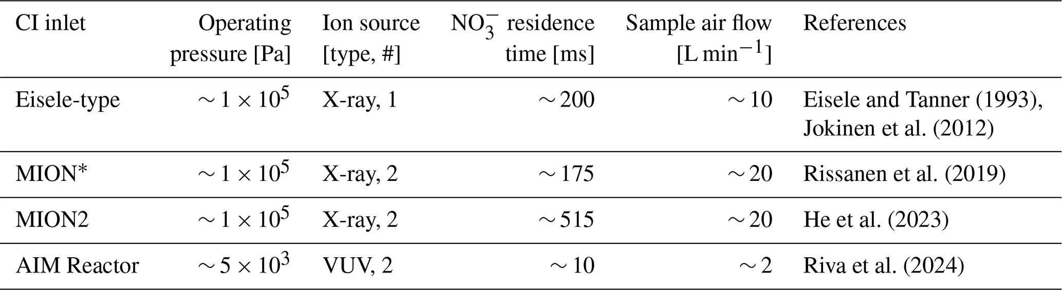
The CI inlets employed during the ACTRIS CI-FI1 campaign (Fig. 1), as well as the APi-ToF and B-ToF mass spectrometers, have been described in dedicated publications, along with their various applications. Here, we report the operating settings applied during the intercomparison campaign (Table 2) and highlight the main differences among the chemical ionization inlets and between the mass analyzers. The relevant references are cited in the respective subsections below and, for the CI inlets, are also listed in Table 2.

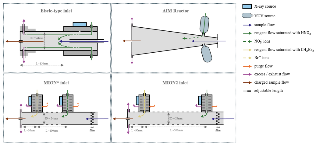
Figure 1 Schematic representation of the chemical ionization inlets employed during the ACTRIS CI-FI1 campaign: Eisele-type inlet, AIM Reactor, MION^∗ inlet, and MION2 inlet. The MION^∗ inlet incorporates an added purge flow compared to the original MION design described by Rissanen et al. (2019), and is therefore denoted with an asterisk.

Table 2 Operating parameters of the CI inlets used during the ACTRIS CI-FI1 campaign, including inlet pressure, ion source type, residence time of NO${}_{\mathrm{3}}^{-}$ reagent ion, and sample air flow rates.

2.2.1 Atmospheric-pressure chemical ionization inlets

The Eisele-type inlet (Eisele and Tanner, 1993; Jokinen et al., 2012) consists of two concentric laminar-flow regions: an outer (O) region, directly exposed to the ionization source, where reagent ions are generated, and an inner (I) region, where these ions react with the sample molecules. Sample air is drawn into the I region through a $\mathrm{3}/\mathrm{4}$ in. stainless steel tube at a flow rate of approximately 10 L min⁻¹. In the O region, around 20 L min⁻¹ of sheath flow (clean air) is mixed with 5–10 mL min⁻¹ of air saturated with the reagent gas. In the inlets used during the ACTRIS CI-FI1 campaign, soft X-ray ionization (Hamamatsu L12535, 4.9 kV) is used to convert reagent molecules into reagent ions. Two coordinated voltages guide the reagent ions from the O region into the I region, while keeping neutral compounds in the O region. There, the reagent ions are electrostatically directed into the sample flow and have a residence time typically ranging from 100 to 300 ms, depending on the setup, during which they interact with the sample molecules.

The MION^∗ inlet used in this study is an upgraded version of the MION inlet presented by Rissanen et al. (2019). It consists of an electrically grounded laminar flow tube with a 24 mm inner diameter, designed to accommodate multiple ion sources; in the present setup, two sources were employed, one for NO${}_{\mathrm{3}}^{-}$ and one for Br⁻. Approximately 20 L min⁻¹ of sample air is drawn into the flow tube after passing through an upstream ion filter that removes any pre-existing ions from the sample air. A gas-phase stream of clean air, ranging from 5 to 50 mL min⁻¹ depending on the reagent gas, is used to deliver the reagent gas through the dedicated ion source, where it is ionized by soft X-ray radiation (Hamamatsu L12535, 4.9 kV). The resulting reagent ions are accelerated and focused by electric fields through 5 mm orifices into the flow tube, where they interact with the laminar sample flow. Each ion source includes a purge flow, consisting of the same air stream used for the reagent flow, which (1) prevents neutral reagent gases from entering the sample flow, and (2) avoids the backflow of sample air into the ion source. The residence time of reagent ions in the flow tube depends on the distance between the ion source and the mass spectrometer pinhole, and thus differs between the two ion sources. Under the configuration used during this campaign, the residence time was ∼ 175 ms for the upstream reagent (NO${}_{\mathrm{3}}^{-}$) and ∼ 40 ms for the downstream reagent (Br⁻).

The MION2 inlet (He et al., 2023) differs from MION^∗ in one respect: it allows for the operation of up to three ion sources placed at equal distance from the pinhole. Additionally, the connecting pipe lengths can be adjusted both between the upstream source and the instrument pinhole and between the upstream and downstream sources, providing flexibility in setting the residence times of both reagent ions, unlike in MION^∗, where the closest source is fixed in position. In the setup used during this campaign, only two ion sources were operated, one for NO${}_{\mathrm{3}}^{-}$ and one for Br⁻. The sources were separated by ∼ 350 mm, resulting in a residence time of ∼ 515 ms for NO${}_{\mathrm{3}}^{-}$ and ∼ 40 ms for Br⁻.

2.2.2 Low-pressure chemical ionization inlet

The Vocus AIM Reactor (Riva et al., 2024) operates at sub-atmospheric (medium) pressures, typically around 50 mbar and within a range of 20–500 mbar, and it further differs from the atmospheric-pressure CI inlets described in Sect. 2.2.1 in that all surfaces in contact with the sample before entering the inlet are made of Teflon^® rather than stainless steel. Sample air is introduced into the reactor at a flow rate of approximately 2 L min⁻¹. Reagent ions are generated using compact vacuum ultraviolet (VUV; UV lamp krypton DC PID PKS 106, Heraeus) ion sources, with reagent gas delivered through the ion source and into the ion–molecule reaction (IMR) region at a flow rate of about 0.25 L min⁻¹. Similar to the MION inlets, the AIM Reactor can accommodate multiple ion sources, allowing up to three sources to be arranged radially. In the configuration used in this study, two sources were implemented, injecting reagent ions at an angle of approximately 45° relative to the sample flow. The reactor temperature is actively controlled and typically maintained at 50 °C to ensure stable reaction conditions. Under these operating conditions, the residence time of reagent ions is on the order of ∼ 10 ms.

2.2.3 Atmospheric Pressure interface Time-of-Flight mass spectrometer

The APi-ToF is a high-resolution mass spectrometer capable of detecting natural ions with minimal fragmentation, limited to weakly bound clusters. The instrument has been described in detail by Junninen et al. (2010), and a brief overview is also provided in Sect. S4 in the Supplement. For the purposes of this intercomparison, it is sufficient to highlight that the key difference between H-ToF and L-ToF mass analyzers lies in the length of the ToF chamber – 665 and 1330 mm, respectively – which directly affects mass resolving power: a longer flight path allows for better separation of ions, thus resulting in higher resolution. According to specifications from Tofwerk AG, the theoretical mass resolution ranges from 3000–7000 Th $/$ Th for H-ToF and up to 6000–14 000 Th $/$ Th for L-ToF.

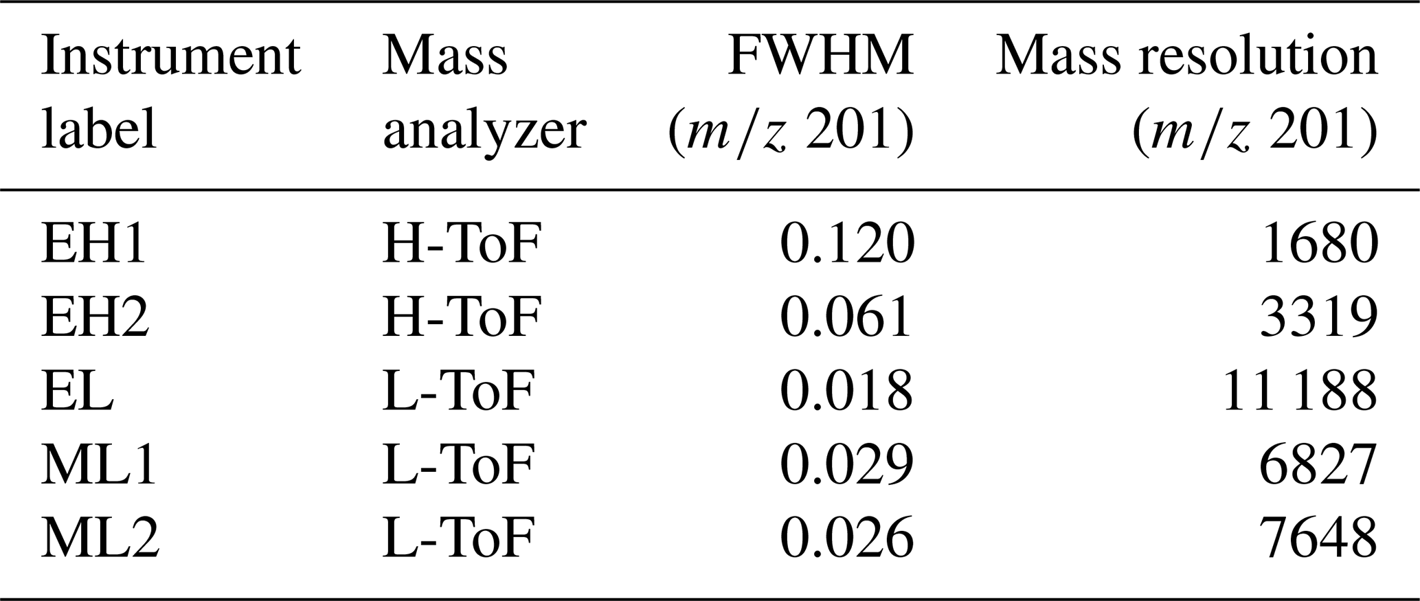
For the NO${}_{\mathrm{3}}^{-}$ mode measurements presented in this study, the mass resolution at $m/z$ = 201, calculated from the full width at half maximum (FWHM) of the corresponding peak, is reported for each CI-APi-ToF in Table 3.

Table 3 Full width at half maximum (FWHM) and corresponding mass resolution at $m/z$ = 201 (nitrate mode) for the five CI-APi-ToF mass spectrometers included in the intercomparison study.

2.2.4 Bipolar Time-of-Flight mass spectrometer

The Vocus B4 is a bipolar time-of-flight mass spectrometer in which sample ions are transmitted through a common, differentially pumped vacuum interface before entering polarity-specific ToF paths. Unlike single-analyzer instruments (e.g., APi-ToF), polarity switching in the Vocus B4 does not require switching of the high voltages of the ToF chambers or detectors. Instead, the positive- and negative-ion ToF chambers remain operated at their respective high-voltage settings, while fast switching of low voltages (those of the interface) selects the transmitted polarity or reagent ion mode. This enables the quasi-simultaneous detection of positive and negative ions, with polarity switching on the order of 50 ms. Being L-ToF analyzers, both ToF chambers achieve a theoretical mass resolution of ∼ 10 000 Th $/$ Th.

2.2.5 Reagent ion chemistry

All the instruments involved in the ACTRIS CI-FI1 campaign operated with nitric acid (HNO₃) either as the sole or as one of the reagent gases. When HNO₃ is used, the ionization predominantly generates nitrate ion clusters, (HNO₃)_xNO${}_{\mathrm{3}}^{-}$ (x = 0–2; Ehn et al., 2014; Jokinen et al., 2012). These reagent ions are highly selective toward H₂SO₄ and other gas-phase acids stronger than HNO₃, as well as toward oxidation products of VOCs containing more than five oxygen atoms, with the binding strength of the reagent ion to the target molecule increasing almost linearly with the number of oxygen atoms (Hyttinen et al., 2018). In the first case, the acids are directly ionized and detected either as single deprotonated ions or as clusters with HNO₃. In the second case, the detection of such highly oxygenated species relies primarily on clustering with NO${}_{\mathrm{3}}^{-}$ via collisions with nitrate ion clusters, through a ligand exchange reaction (Hyttinen et al., 2015, 2018).

Instruments ML1 and ML2 also employed a second reagent gas, dibromomethane (CH₂Br₂), whose ionization primarily produces Br⁻, with Br${}_{\mathrm{3}}^{-}$ formed to a lesser extent through Br₂-Br⁻ recombination (Finkenzeller et al., 2024). In this case, the analyte is charged via direct adduct formation with Br⁻ (Hyttinen et al., 2018). Although this ionization method is less selective than NO${}_{\mathrm{3}}^{-}$, it has proven suitable for studying atmospheric organic compounds that are less oxidized than those typically favored by NO${}_{\mathrm{3}}^{-}$ (Huang et al., 2021; Rissanen et al., 2019). Moreover, Br⁻ ionization has been applied to the detection of OH and hydroperoxyl radicals (HO₂; Albrecht et al., 2019; Lambe et al., 2022; Sanchez et al., 2016), as well as halogenated compounds (Wang et al., 2021). Finally, Br⁻ shares with NO${}_{\mathrm{3}}^{-}$ the capability to detect H₂SO₄ (Wang et al., 2021), which makes it quantitatively comparable to the nitrate ion chemistry.

Instrument AB employed two additional reagent gases alongside HNO₃: methyl iodide (CH₃I) and benzene (C₆H₆), which are ionized to I⁻ and (C₆H₆)${}_{\mathrm{2}}^{+}$, respectively. The ionization pathways and target compound classes of I⁻ largely overlap with those of Br⁻, although I⁻ forms weaker adducts with the analytes (Hyttinen et al., 2018). As for (C₆H₆)${}_{\mathrm{2}}^{+}$ mode, it predominantly targets volatile precursor species of condensable vapors, such as isoprene and terpenes (Lavi et al., 2018) or dimethyl sulfide (Kim et al., 2016). In the present work, only iodide-mode data are discussed for instrument AB.

2.3 Data analysis

2.3.1 Selected peak list

The target species considered in this study were selected among condensable vapors involved in the different stages of NPF, and were based on two main criteria: the measurement site (i.e., a boreal forest environment), and the selectivity of the reagent ions employed (Sect. 2.2.5).

The shortlist of peaks selected for NO${}_{\mathrm{3}}^{-}$ mode (Table S2 in the Supplement) includes sulfuric acid, a few strong organic and inorganic acids (hereafter referred to as HA), as well as several monoterpene-derived HOMs belonging to different chemical classes, namely organic peroxy radicals, closed shell non-nitrate monomers, closed shell organonitrate monomers, and dimers. All selected species contain seven or more oxygen atoms, for which NO${}_{\mathrm{3}}^{-}$ shows high selectivity.

The peak list used for Br⁻ mode (Table S3 in the Supplement) includes the same species as in NO${}_{\mathrm{3}}^{-}$ ion mode, with NO${}_{\mathrm{3}}^{-}$ in the clusters replaced by Br⁻ and the corresponding reagent ions adjusted accordingly. However, due to the higher sensitivity of Br⁻ toward less oxidized acids, a set of additional organic compounds containing three to six oxygen atoms were included in both the nitrate and bromide peak lists to enable a more meaningful comparison between the two reagent ion modes in instruments operating with both. These species were classified as semi-volatile organic compounds (SVOCs) according to the parametrization proposed by Donahue et al. (2011) and later updated by Mohr et al. (2019).

Finally, among the peaks fitted in I⁻ mode, only six species were selected for this study, corresponding to compounds already included in the other two peak lists within the SVOC group, detected here as clusters with I⁻ (Table S4 in the Supplement).

2.3.2 Sulfuric acid calibration

The method for sulfuric acid calibration of chemical ionization mass spectrometers, introduced by Kürten et al. (2012), was applied to each CI-APi-ToF during the campaign using the same setup. The calibration factor, C_SA, was determined from the slope of the linear regression between the modeled H₂SO₄ concentration and the reagent ion normalized H₂SO₄ signal, $S_{{\mathrm{H}}_{\mathrm{2}}{\mathrm{SO}}_{\mathrm{4}}}$, at different calibration steps. The modeled H₂SO₄ concentration for each calibration step was calculated using a dedicated MATLAB model, while the normalized H₂SO₄ signal in nitrate mode was calculated according to Eq. (1):

$$\begin{array}{}\text{(1)}& \begin{array}{rl}& S_{{\mathrm{H}}_{\mathrm{2}}{\mathrm{SO}}_{\mathrm{4}}}=\\ & {\displaystyle \frac{{\mathrm{HSO}}_{\mathrm{4}}^{-}+{\mathrm{HNO}}_{\mathrm{3}}\cdot {\mathrm{HSO}}_{\mathrm{4}}^{-}+{\mathrm{H}}_{\mathrm{2}}{\mathrm{SO}}_{\mathrm{4}}\cdot {\mathrm{HSO}}_{\mathrm{4}}^{-}}{{\mathrm{NO}}_{\mathrm{3}}^{-}+{\mathrm{HNO}}_{\mathrm{3}}\cdot {\mathrm{NO}}_{\mathrm{3}}^{-}+({\mathrm{HNO}}_{\mathrm{3}}{)}_{\mathrm{2}}\cdot {\mathrm{NO}}_{\mathrm{3}}^{-}+{\mathrm{H}}_{\mathrm{2}}\mathrm{O}\cdot {\mathrm{NO}}_{\mathrm{3}}^{-}}}.\end{array}\end{array}$$

During the ACTRIS CI-FI1 campaign, sulfuric acid calibrations were conducted in five steps, each lasting 10 min. For all instruments, signals were averaged over 2 min intervals. The calibration was not performed for instrument AB, since it was not expected to detect H₂SO₄ at the low concentrations typical of the measurement site.

Since both nitrate and bromide ionization detect H₂SO₄ near collision limit (Ehn et al., 2014; Wang et al., 2021), sulfuric acid is considered a suitable calibration compound also when operating in this second reagent ion mode. The equation used to calculate the Br⁻ mode normalized H₂SO₄ signal is provided in the Supplement (Sect. S8), along with a detailed description of the calibration setup employed during the campaign (Sect. S7).

2.3.3 Transmission calibration

In cases where a direct calibration method for the target compound has not yet been established, the accurate quantification of the analyte requires knowledge of the transmission efficiency of the instrument (Alfaouri et al., 2025). In APi-ToF, the unequal transmission of ions depending on their $m/z$, known as mass discrimination, occurs primarily in the first two quadrupoles of the APi section, the ToF orthogonal extraction unit, and the microchannel plate (MCP) detector (Heinritzi et al., 2016). When a CI source is used upstream of the APi-ToF, the transmission of an ion at a given $m/z$ can be determined relative to that of the reagent ion.

Table 4 Perfluorinated acids used for the transmission calibrations.

Transmission calibrations were performed on all CI-APi-ToFs in NO${}_{\mathrm{3}}^{-}$ mode, following the depletion method described by Heinritzi et al. (2016), and briefly here. A Union Tee piece of $\mathrm{3}/\mathrm{4}$ in. was attached to the inlet tubes of the CI-APi-ToFs, using adaptors to 1 in. for instruments with larger inlet tube diameter. The third outlet of the Tee was closed with a cap, in which a small quantity of the perfluorinated acids used for the calibration was placed, either in liquid or solid form, one compound at a time. The calibration experiment consisted of heating the cap with a heat gun to induce evaporation or sublimation of the calibrant, resulting in depletion of the reagent ions. After the heating cycle, the signal from the perfluorinated acid decreased as the system cooled and the primary reagent ions recovered. The perfluorinated acids used in the experiments are listed in Table 4. During the ACTRIS CI-FI1 campaign, C5 and C7 were employed, with C7 excluded for EH2, whereas C7, C8, and C9 were used for ML2, which was calibrated post-campaign in the ACTRIS Laboratory of the University of Helsinki. The use of different calibrant sets was mainly related to time limitations during the campaign, as well as to ongoing testing and optimization of the method. Based on the experience gained during the campaign, we recommend performing at least three heating cycles for each calibrant and aiming for different degrees of reagent ion depletion, as also suggested by Heinritzi et al. (2016).

Curves describing the relative transmission as a function of $m/z$ were derived by least-squares fitting of a 2-fold Gaussian distribution (Eq. 2) to the depletion experiment data:

$$\begin{array}{}\text{(2)}& \begin{array}{rl}f\left(x\right)=& a_{\mathrm{1}}\cdot \exp \left(-{\left({\displaystyle \frac{x-b_{\mathrm{1}}}{c_{\mathrm{1}}}}\right)}^{\mathrm{2}}\right)\\ & +a_{\mathrm{2}}\cdot \exp \left(-{\left({\displaystyle \frac{x-b_{\mathrm{2}}}{c_{\mathrm{2}}}}\right)}^{\mathrm{2}}\right),\end{array}\end{array}$$

where x corresponds to the $m/z$ of the selected species. Following Heinritzi et al. (2016), lower limits were imposed on the two parameters in the denominator of the exponential term (c₁, c₂ ≥ 200) to ensure a more robust representation of the measured data. Additionally, since the instruments were calibrated using H₂SO₄, the relative transmission for all peaks contributing to the H₂SO₄ signal was constrained to unity. As all peaks associated with the selected HA species are in same mass range as sulfuric acid peaks ($m/z$ = 97, 160, and 195), we assume, as an approximation, that their relative transmission is likewise equal to 1. Therefore, no transmission correction factor, C_trans, is applied to these species (see Eq. 4), as it is also the case for H₂SO₄ (see Eq. 3).

Since the relative transmission curve describes the mass-dependent discrimination of analyte ions relative to that of the reagent ions, its applicability to other ionization modes must be carefully considered. The comparable binding strengths of NO${}_{\mathrm{3}}^{-}$ and Br⁻ to oxidized molecules (Hyttinen et al., 2018) suggests that the corresponding clusters with HOMs are detected with similar efficiency under the same mass spectrometer settings (Rissanen et al., 2019). Therefore, the transmission curve obtained from the calibrations performed in NO${}_{\mathrm{3}}^{-}$mode was applied to Br⁻ mode measurements as well.

2.3.4 Data processing

Ambient data, background measurement data, and sulfuric acid calibration data were processed using the Tofware analysis software package, while transmission calibration data were processed using the MATLAB-based tofTools software, as the functions used for deriving transmission curves were implemented in MATLAB.

Signals from ambient measurements were pre-averaged over 10 min intervals for all CI-APi-ToFs, regardless of their individual acquisition time. This averaging time was selected to better reflect typical data processing practices for these instruments during field measurements, where, depending on the application, averaging times of 30 or even 60 min are commonly used. In this campaign, instruments ML1 and ML2 alternated ionization modes every 10 min, which made the choice of 10 min pre-averaging convenient for the purposes of the study. As described in Sect. 2.3.2, sulfuric acid calibration data were treated differently and averaged over 2 min intervals. This choice was related to the 10 min duration of each calibration step: since the signal is often not stable during the initial part of each step, 2 min averaging provides enough data points per step when evaluating the time series of the sulfuric acid signal. Background measurement data were also averaged over 2 min intervals, for consistency with the sulfuric acid calibration data. This was also motivated by the relatively short duration of the background measurements (∼ 30 min), since using longer averaging times, such as 10 min as for the ambient data, would have resulted in too few data points.

In NO${}_{\mathrm{3}}^{-}$ mode, H₂SO₄ and the other strong acids were quantified using Eqs. (3) and (4), respectively. Selected HOM species were quantified using Eq. (5) and subsequently grouped by chemical class (Tables S2–S4 in the Supplement).

$$\begin{array}{}\text{(3)}& {\displaystyle }\left[{\mathrm{H}}_{\mathrm{2}}{\mathrm{SO}}_{\mathrm{4}}\right]=S_{{\mathrm{H}}_{\mathrm{2}}{\mathrm{SO}}_{\mathrm{4}}}\times C_{\mathrm{SA}},\text{(4)}& {\displaystyle }\begin{array}{rl}\left[\mathrm{HA}\right]=& {\displaystyle \frac{A^{-}+{\mathrm{HNO}}_{\mathrm{3}}\cdot A^{-}}{\left(\begin{array}{c}{\mathrm{NO}}_{\mathrm{3}}^{-}+{\mathrm{HNO}}_{\mathrm{3}}\cdot {\mathrm{NO}}_{\mathrm{3}}^{-}+\\ {\left({\mathrm{HNO}}_{\mathrm{3}}\right)}_{\mathrm{2}}\cdot {\mathrm{NO}}_{\mathrm{3}}^{-}+{\mathrm{H}}_{\mathrm{2}}\mathrm{O}\cdot {\mathrm{NO}}_{\mathrm{3}}^{-}\end{array}\right)}}\\ & \times C_{\mathrm{SA}}\times C_{\mathrm{inlet}},\end{array}\text{(5)}& {\displaystyle }\begin{array}{rl}\left[\mathrm{HOM}\right]=& {\displaystyle \frac{\mathrm{HOM}\cdot {\mathrm{NO}}_{\mathrm{3}}^{-}}{\left(\begin{array}{c}{\mathrm{NO}}_{\mathrm{3}}^{-}+{\mathrm{HNO}}_{\mathrm{3}}\cdot {\mathrm{NO}}_{\mathrm{3}}^{-}+\\ {\left({\mathrm{HNO}}_{\mathrm{3}}\right)}_{\mathrm{2}}\cdot {\mathrm{NO}}_{\mathrm{3}}^{-}+{\mathrm{H}}_{\mathrm{2}}\mathrm{O}\cdot {\mathrm{NO}}_{\mathrm{3}}^{-}\end{array}\right)}}\\ & \times C_{\mathrm{SA}}\times C_{\mathrm{inlet}}\times C_{\mathrm{trans}}.\end{array}\end{array}$$

In the equations above, C_SA, represents the calibration factor derived from the sulfuric acid calibration described in Sect. 2.3.2. The sulfuric acid concentration is derived using the same set of peaks as those used to calculate $S_{{\mathrm{H}}_{\mathrm{2}}{\mathrm{SO}}_{\mathrm{4}}}$ during the calibration. For species other than sulfuric acid, C_inlet accounts for diffusional losses of the sample in the inlet tube and it is calculated based on species-specific gas diffusion coefficients, estimated following the approach of Fuller et al. (1966, 1969; Sect. S6 in the Supplement). Finally, C_trans is the mass-dependent transmission correction factor, obtained as the inverse of the relative transmission function fitted for each instrument and resolved for each species as detailed in Sect. 2.3.3. For H₂SO₄, C_SA intrinsically includes both inlet loss and transmission correction factors (Heinritzi et al., 2016; Kürten et al., 2012). For HAs and HOMs, C_inlet and C_trans are calculated relative to H₂SO₄, which serves as the calibration reference.

Analogous equations were applied to Br⁻ mode data (Sect. S8 in the Supplement).

The AB instrument data were treated separately. Analyte signals were processed by normalizing them to respective reagent ion count rate of 1 million counts s⁻¹, as measured at the detector (Lee et al., 2014). This normalization was applied to account for variations in instrument response caused by changes in ion source intensity and detector gain. For compounds that were not directly calibrated, concentrations were estimated using the collision-limited sensitivity of 10 ncps ppt⁻¹ to convert normalized signals to mixing ratios (Aggarwal et al., 2025)

2.3.5 Background measurements and detection limit

Background measurements in NO${}_{\mathrm{3}}^{-}$mode were performed for all CI-APi-ToFs by connecting a high-efficiency particulate air (HEPA) filter (Cytiva HEPA Capsule Versapor™ 1.2 µm HB, 1 pack) to the inlet tube and sampling for approximately 30 min. The use of HEPA filter for this type of measurements has been reported in previous studies (Boyer et al., 2024; Häkkinen et al., 2023) and is straightforward to apply during field measurements. Although HEPA filters are conventionally used to remove particles in particle-phase measurements, they can also be used for background measurements of gas-phase species when the compounds of interest are sufficiently low volatile and are efficiently removed by interaction with the filter material. The efficiency of this removal is, however, compound-dependent and the filter should therefore not be considered a universal gas-phase zeroing method. To demonstrate the effectiveness of the approach for the compounds targeted in this study, measurements with and without the HEPA filter are shown in Fig. S3 in the Supplement. The signals of the investigated compounds were strongly suppressed when the filter was installed, although the signals did not decrease completely to zero and the extent of signal decrease differed among sulfuric acid, HAs, and HOMs.

The limit of detection (LOD), defined as the minimum analyte signal that can be distinguished from background noise, can be determined using different approaches. Here, following He et al. (2023), the LOD for H₂SO₄ was calculated as:

$$\begin{array}{}\text{(6)}& {\mathrm{LOD}}_{\mathrm{SA}}=\left(\mathit{\mu }+\mathrm{3}\mathit{\sigma }\right)\cdot C_{\mathrm{SA}},\end{array}$$

where μ represents the mean value of the normalized sulfuric acid signal during the background measurement, and σ is the corresponding standard deviation. As described by He et al. (2023), for species without a direct calibration, such as HOMs, the LOD calculated using the sulfuric acid calibration factor can be applied, although this generally represents a lower limit of the actual LOD.

To further characterize differences in noise levels between instruments, we calculated a more general LOD, referred to as LOD_CIMS, using the same formula but a different definition of μ: for each HOM peak included in the NO${}_{\mathrm{3}}^{-}$mode peak list, a nearby region where no peak was expected was selected, and the signal in this region was fitted and taken as μ. For example, for a peak at nominal masses 308 and 494 Th, the signal at 308.5 and 494.5 Th were used, and similarly for other peaks up to a nominal mass of 620 Th. Since the HOM peaks span a broad $m/z$ range, LOD_CIMS arguably provides a more general characterization of the background signal and noise level, rather than a compound-specific detection limit, such as LOD_SA, and can thus help in interpreting differences in measurement outcomes between instruments. It should be noted that the detection limit of an individual compound can also be affected by the presence and intensity of nearby peaks, an effect that is not accounted for in this approach and may become increasingly relevant at higher $m/z$.

Under the relatively clean conditions of the SMEAR II station and during rainy days with limited photochemical activity, the ambient concentrations of sulfuric acid and other analytes were generally low. This made the measurements challenging for all instruments, with several data points approaching the detection limits, but the situation was particularly critical for the AB instrument, for which the lower pressure of the AIM inlet inherently affects sensitivity and increases detection limits. Consequently, the NO${}_{\mathrm{3}}^{-}$ mode did not perform well for this instrument, possibly further affected by contamination issues in the bipolar configuration during the campaign. For this reason, NO${}_{\mathrm{3}}^{-}$ mode data from AB were excluded from the intercomparison (Sect. 3.3), and the focus was instead on I⁻ mode measurements. Accordingly, LOD_SA and LOD_CIMS were not calculated for this instrument.

3 Results and discussion

3.1 Sulfuric acid calibration factor and detection limit

Table 5 collects C_SA values resulting from the sulfuric acid calibrations (Sect. 2.3.2), along with the LOD_SA and LOD_CIMS values calculated based on the background measurements (Sect. 2.3.5). NO${}_{\mathrm{3}}^{-}$ mode C_SA values generally lie in the range 1–2 × 10¹⁰ cm⁻³, with the exception of EL, which shows a calibration factor of 7.25 × 10⁹ cm⁻³. The highest C_SA is that of EH2, which also exhibits the highest inlet losses, likely due to its comparatively narrower and longer inlet tube combined with a lower inlet flow rate (Zhang et al., 2023). Nevertheless, LOD_SA values calculated for all instruments are fairly similar, ranging between 1–3 × 10⁵ cm⁻³, with ML2 showing the lowest detection limit for H₂SO₄. LOD_CIMS values, instead, are about one order of magnitude lower than LOD_SA values, and ML2 again shows a notably lower detection limit. Although the ranking of the instruments based on LOD_SA and LOD_CIMS is not identical, EH1 and EH2 show overall higher background noise throughout the mass spectrum, while ML2 consistently exhibits lower detection limits compared to the other instruments.

Table 5 Sulfuric acid calibration factors and detection limits calculated for the five CI-APi-ToFs, reported alongside selected inlet parameters. The C_SA value reported for ML1 operating in Br⁻ mode corresponds to the revised calibration factor ($C_{\mathrm{SA}}^{\prime }$).

The LOD_CIMS values obtained here are overall comparable to the detection limit of 3.6 × 10⁴ cm⁻³ reported by Jokinen et al. (2012) for 15 min averaged NO${}_{\mathrm{3}}^{-}$ mode measurements with a CI-APi-ToF. By contrast, the LOD_SA values obtained in this study are higher than the compound-specific sulfuric acid detection limits of 7.6 × 10⁴ and 8.8 × 10⁴ cm⁻³ reported by He et al. (2023) and Boyer et al. (2024), respectively. However, differences in the background measurement procedure and averaging time need to be considered when comparing these values. Boyer et al. (2024) used HEPA-filter background measurements, as in the present study, and 5 min averaged data, whereas He et al. (2023) introduced pure nitrogen or synthetic air into the CI inlet and calculated the LOD from 1 h of data averaged to 1 min intervals. In addition, possible incomplete removal of sulfuric acid or sulfuric-acid-containing clusters during HEPA-filter background measurements may have contributed to an overestimation of the derived LOD_SA values. For these reasons, the reported LOD values should not be considered strict limits below which the measurements are necessarily unreliable.

For ML1 and ML2, C_SA values obtained in Br⁻ mode are higher than those in NO${}_{\mathrm{3}}^{-}$ mode. This is consistent with the different ion chemistry of NO${}_{\mathrm{3}}^{-}$ and Br⁻ toward H₂SO₄, with NO${}_{\mathrm{3}}^{-}$ providing higher sensitivity and therefore lower calibration factors. The longer residence time of the NO${}_{\mathrm{3}}^{-}$ source may also partially contribute to this difference.

We note that for ML1 operated in Br⁻ mode, the sulfuric acid calibration was performed following an abrupt shift in the ML1 bromide reagent ions behavior that occurred on 31 July; consequently, the data acquired thereafter in this mode are not considered reliable for the remainder of the ACTRIS CI-FI1 campaign. The calibration factor derived from this experiment was therefore not used in the analysis. Instead, a revised calibration factor, $C_{\mathrm{SA}}^{\prime }$, was derived from the two neighboring calibrations obtained for this instrument with the same experimental setup, one before the campaign and one following the campaign, when the Br⁻ mode was operating properly. This highlights the importance of regular calibrations, which allowed this deviation from the regular instrument performance to be identified and addressed. Additional details are given in Sect. S13 in the Supplement.

3.2 Transmission curves

Figure 2 shows the relative transmission curves for all the CI-APi-ToFs, obtained from the transmission calibrations performed as described in Sect. 2.3.3. With the exception of EH1, the relative transmission increases above unity and reaches its maximum between $m/z$ 400 and 500, before decreasing and approaching zero beyond $m/z$ 800. This trend is especially pronounced for ML2, which shows a peak relative transmission more than twice that of ML1, the instrument with the second-highest maximum. Considering that the HOM clusters we targeted in this study have masses between $m/z$ 240–620 in nitrate mode and $m/z$ 260–640 in bromide mode, we expected improved detectability of both monomers and dimers in instruments exhibiting higher transmission in this mass range, in the order ML2 > ML1 > EL, followed by EH2. The curve obtained for EH1, however, shows a different behavior: the relative transmission never exceeds unity and gradually decreases starting from about $m/z$ 200, approaching zero already around $m/z$ 600. Hence, based on the transmission curve alone, EH1 would be expected to show little to no signal in the mass range of interest.

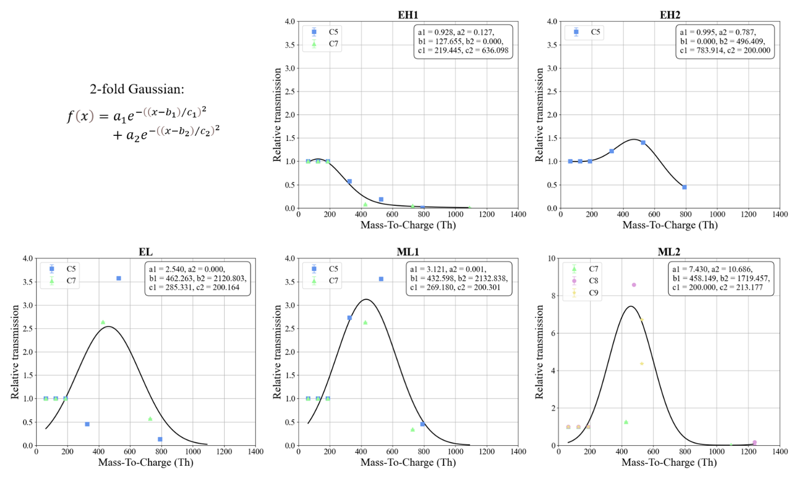
Figure 2 Relative transmission curves derived for all instruments based on the transmission calibrations with perfluoro compound depletion technique (Heinritzi et al., 2016; C5 – blue, C7 – green, C8 – pink, C9 – yellow). The curves were obtained by least-squares fitting of a 2-fold Gaussian function to the depletion data. Note the different y-axis scale for ML2.

Given the peculiar relative transmission curve of EH1, the resulting C_trans for the selected HOMs becomes considerably large, especially for HOM dimers. This occurs because C_trans is calculated as $\mathrm{1}/f\left(x\right)$, and when f(x) is close to zero, the resulting correction factors are unrealistically large relative to actual HOM concentrations. For this reason, the application of the transmission correction factor is arguably unreliable when f(x) is zero or near zero, as it is the case for the EH1 relative transmission function beyond $m/z$ 400.

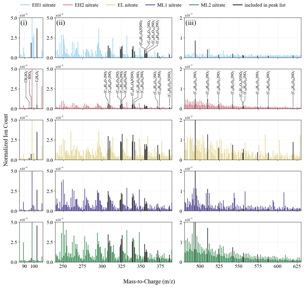
Figure 3 Selected segments of the unit mass resolution (UMR) mass spectra measured by the five CI-APi-ToF mass spectrometers operating in nitrate mode, averaged over four daytime hours (12:00–16:00 LT) during peak photochemical activity on 1 August 2024. Peak intensities were normalized to the reagent ion intensities. The three columns show (i) the range containing the main sulfuric acid signal, corresponding to the bisulfate peak ($m/z$ 97; 85–110), (ii) the region where monoterpene-derived HOM monomers clustered with NO${}_{\mathrm{3}}^{-}$ fall ($m/z$ 240–390), and (iii) the region where monoterpene-derived HOM dimers clustered with NO${}_{\mathrm{3}}^{-}$ appear ($m/z$ 480–630). Each row corresponds to a different mass spectrometer. Peaks corresponding to target species included in the NO${}_{\mathrm{3}}^{-}$ mode peak list are highlighted in black.

To assess whether the derived transmission curves are consistent with the observed mass spectra, we compared the spectra recorded by the different CI-APi-ToFs in the $m/z$ regions relevant for the species targeted in this study. Specifically, we selected three regions: (i) the range containing the main sulfuric acid signal, corresponding to the bisulfate peak ($m/z$ 97; 85–110), (ii) the region where monoterpene-derived HOM monomers clustered with NO${}_{\mathrm{3}}^{-}$ fall ($m/z$ 240–390), and (iii) the region where monoterpene-derived HOM dimers clustered with NO${}_{\mathrm{3}}^{-}$ appear ($m/z$ 480–630). Figure 3 shows the three selected segments of the unit mass resolution (UMR) mass spectra measured by the five mass spectrometers, averaged over four daytime hours (12:00–16:00 LT) during peak photochemical activity on 1 August 2024.

Overall, the figure shows that the instruments do not produce identical mass spectra, even when operated with the same reagent ion. In regions (i) and (ii), the spectra measured by ML1 and ML2 show comparable signal intensities and similar peak patterns. The spectra from EH1 and EL also compare well, although the spectrum measured by EL exhibits slightly higher signal intensity, whereas EH2 shows substantially lower signals in region (ii), consistent with its lower transmission in this mass range compared to the other instruments. In region (iii), the differences between instruments become more pronounced, with EH2 and especially EH1 showing much lower signal intensities compared to ML1 and ML2. This behavior is consistent with the transmission curves shown in Fig. 2, which indicate higher transmission for ML1 and ML2 at such high $m/z$ values.

Table 6 Coefficients of determination (R²) and relative median absolute deviation (rMAD) calculated from concentrations of different HOM classes measured by five CI-APi-ToF mass spectrometers on 1–2 August 2024. Values are shown for cases (a) where only C_SA is applied, (b) where C_SA, C_inlet, and C_trans are applied to all instruments, and (c) where the same corrections are applied to all instruments except EH1.

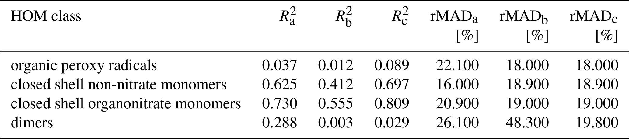
Notably, EH1 still shows a clear signal in region (ii), despite the derived relative transmission curve indicating very low transmission at these $m/z$ values. Thus, we estimated (1) to what extent the application of the transmission correction factor C_trans (together with the inlet loss correction C_inlet) improves the consistency and agreement between measurements from different instruments, and (2) to what extent, in the present case, not applying C_trans to the EH1 measurements improves the agreement compared to applying it. To this end, correlation analysis was performed on concentrations of different HOM classes measured by all CI-APi-ToFs operating in NO${}_{\mathrm{3}}^{-}$ and Br⁻ modes over selected days (1–2 August and 27–31 July, respectively). For nitrate mode, the analysis was conducted by (a) applying only C_SA, (b) applying C_SA, C_inlet, and C_trans to all instruments, and (c) applying the same corrections to all instruments except EH1. In addition to the coefficient of determination (R²), the relative median absolute deviation (rMAD) was calculated to quantify how much the measurements differ between instruments. Table 6 summarizes the results for NO${}_{\mathrm{3}}^{-}$ mode. Figure S4 in the Supplement provides a more immediate visualization of the effect of applying the different correction factors to measurements from the five CI-APi-ToFs operating in nitrate mode.

As shown in Table 6, applying all correction factors to all instruments (case b) generally leads to a decrease in R², indicating reduced consistency among instruments. However, excluding C_trans for EH1 (case c) improves the agreement compared to both case (a) and (b), yielding higher R² values for most HOM groups. Two cases deviate from this general behavior. First, for HOM dimers, the highest R² value is observed in case (a), rather than in case (c). A possible explanation for this unexpected result is discussed in Sect. 3.3. Nevertheless, the rMAD in case (c) is lower than in case (a) and, especially, case (b), indicating improved agreement despite the lower R². Second, for HOM closed shell non-nitrate monomers, R² follows the expected behavior and increases from case (a) to case (c); however, the rMAD increases upon applying the full set of corrections and does not improve when excluding C_trans for EH1. This suggests that the observed variability for this group is not primarily driven by the EH1 transmission correction.

These results indicate that differences in transmission among instruments are not negligible and should generally be considered when interpreting mass spectrometry data. On the other hand, they also highlight the importance of critically evaluating whether a given relative transmission curve is suitable for correction purposes and whether the transmission calibration itself provides a reliable representation of instrument behavior. In the present case, indeed, applying the transmission correction factor to all instruments without such evaluation leads to reduced agreement overall, an effect that can be attributed primarily to EH1 (Sect. S10 in the Supplement). Therefore, based on all the considerations presented in this section, C_trans was applied to all CI-APi-ToFs except for EH1 data in the subsequent analysis.

3.3 Measurements in nitrate mode

Figure 4 shows sulfuric acid concentrations measured in nitrate mode by the five CI-APi-ToFs participating in ACTRIS CI-FI1 during two days of ambient sampling (1–2 August 2024). The concentrations were calculated according to Eq. (2) and the panels in the two rows (Fig. 4a–c and d–f) present the same analysis but account for two different limits of detection, namely LOD_SA and LOD_CIMS, respectively. Hereafter, we define good agreement as R² > 0.7, moderate agreement that with 0.4 < R² < 0.7, and poor agreement as R² < 0.4.

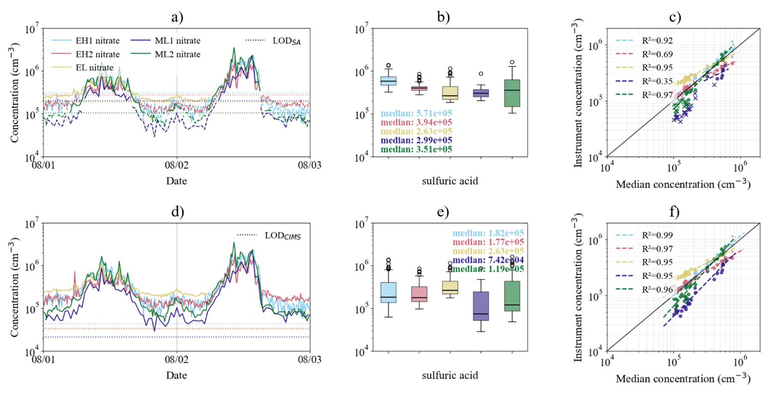
Figure 4 Sulfuric acid concentrations measured in nitrate mode by five CI-APi-ToFs during 1–2 August 2024. Upper and lower panels show the same comparison using two different limits of detection: LOD_SA in the upper panels (a–c) and LOD_CIMS in the lower panels (d–f). For each panel, the left panels (a, d) show the time series of sulfuric acid concentrations, with instrument-specific LOD values indicated by dotted horizontal lines. The central panels (d, e) show a box plot summarizing the distributions over the same period; boxes indicate the interquartile range, horizontal lines indicate the median, whiskers represent the non-outlier range, and empty circles denote outliers. Data points below LOD are excluded from the box plot. The right panels (c, f) show the hourly median sulfuric acid concentration measured by each instrument against the median of the hourly median concentrations across all five instruments. Dashed lines indicate log–log linear regressions for each instrument, with the corresponding coefficient of determination (R²) reported in the legend. Points below the corresponding LOD are shown as crosses (X), while outliers are plotted as smaller semi-transparent points; both are excluded from the linear fits.

The instruments show good agreement during periods of peak H₂SO₄ concentrations in the central part of the day, whereas larger differences are observed at lower H₂SO₄ concentrations. Specifically, in the latter case, the time series show higher signal for the instruments with Eisele-type inlets compared to those with MION inlets. This is further confirmed by the scatter plots: when the concentration measured by an individual instrument is plotted against the median concentration reported by the five instruments, the data points are arranged in a fan-like pattern, with increasing dispersion toward lower concentrations. Consistent with the time series, at lower concentrations the data points from different instruments cluster according to inlet type, with similar distributions observed for Eisele-type inlets and for MION inlets.

To explain this difference in behavior, we examined the detection limits calculated for the five instruments in NO${}_{\mathrm{3}}^{-}$ mode. For sulfuric acid, two definitions of detection limit were considered: LOD_SA, a compound-specific detection limit calculated for each instrument according to Eq. (6), and LOD_CIMS, a background noise level derived following the procedure described in Sect. 2.3.5. As discussed in Sect. 3.1, EH1 and EH2 show higher detection limits than ML1 and ML2 in both cases, consistent with the behavior observed in the time series. In contrast, the detection limit calculated for EL is comparatively low, lying within the range of the other instruments (for LOD_CIMS) or even below ML1 (for LOD_SA), despite the higher background signal observed in the time series. One possible explanation is that the C_SA value for EL is underestimated relative to the calibration factors of the other instruments: since this parameter is included in the LOD calculation, such an underestimation could lead to an apparently lower detection limit. However, if C_SA were indeed significantly underestimated, larger discrepancies in the sulfuric acid concentrations measured by EL would also be expected at higher concentrations, which is not observed.

Notably, when considering LOD_SA, only the sulfuric acid concentrations measured by EL remain above the detection limit over the period considered, although they approach it during nighttime, whereas measurements from all other instruments fall clearly below it. When applying LOD_CIMS, however, measurements from all instruments are above the detection limit. Since measurements below the detection limit are typically excluded from statistical analyses, these differences can directly affect the measurement outcome and interpretation. This highlights the need for a more rigorous and consistent definition of detection limit within the CIMS community.

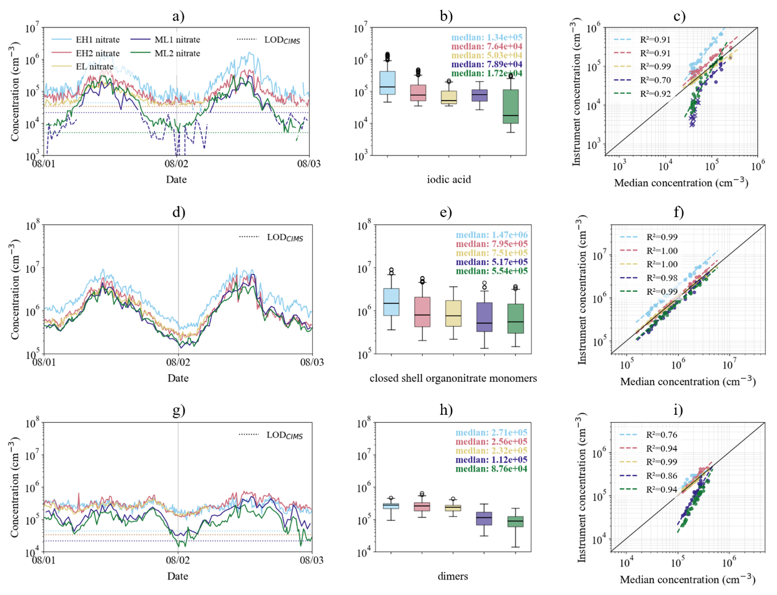
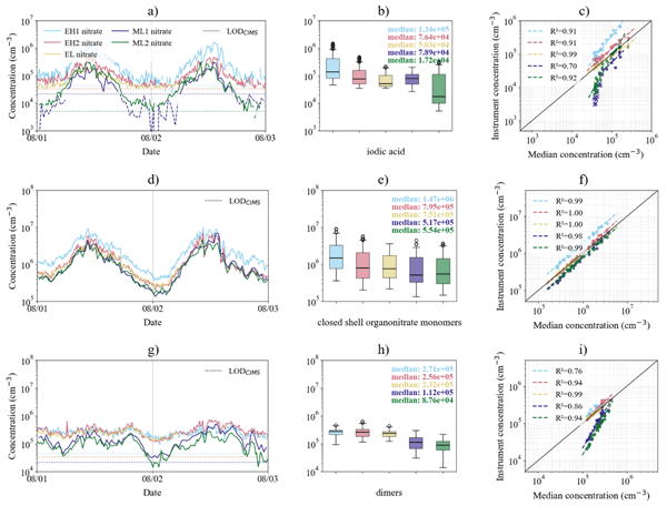
Figure 5 Concentrations of (a–c) iodic acid, (d–f) closed shell organonitrate monomers, and (g–i) dimers measured in nitrate mode by five CI-APi-ToFs during 1–2 August 2024. For each panel, the left panels (a, d, g) show concentration time series, with instrument-specific LOD_CIMS values indicated by dotted horizontal lines. The central panels (b, e, h) show a box plot summarizing the distributions over the same period; boxes indicate the interquartile range, horizontal lines indicate the median, whiskers represent the non-outlier range, and empty circles denote outliers. Data points below LOD_CIMS are excluded from the box plot. The right panels (c, f, i) show the hourly median concentration measured by each instrument against the median of the hourly median concentrations across all five instruments. Dashed lines indicate log–log linear regressions for each instrument, with the corresponding coefficient of determination (R²) reported in the legend. Points below the corresponding LOD_CIMS are shown as crosses (X), while outliers are plotted as smaller semi-transparent points; both are excluded from the linear fits.

Similarly to Fig. 4, Fig. 5 shows concentrations of iodic acid, closed shell organonitrate monomers, and dimers during the selected days. Analogous figures for other HAs and HOM classes are provided in Sect. S11 the Supplement. Iodic acid concentrations were calculated according to Eq. (4), whereas HOM concentrations were calculated according to Eq. (5); for EH1, the C_trans factor was not applied in this case (Sect. 3.2).

The difference at low analyte concentrations between instruments with Eisele-type inlets and to those with MION inlets is even more pronounced for iodic acid (Fig. 5a–c) than for sulfuric acid. Most instruments report higher concentrations in close agreement, with the exception of EH1. At lower concentrations, however, a clear separation of roughly one order of magnitude is observed.

Closed shell organonitrate monomers (Fig. 5d–f), selected across the $m/z$ range 339–387, show a similar behavior. In this case, however, agreement at peak concentrations is even stronger, while differences at lower concentrations are considerably smaller than for iodic acid.

For the dimers (Fig. 5g–i), all plots clearly show the separation between instruments with Eisele-type and MION inlets. Furthermore, the box plots suggest that ML1 and ML2 more effectively distinguish this group of HOMs from the background noise, as the difference between higher and lower concentrations is larger, consistent with an improved signal-to-noise ratio in the $m/z$ range 494–620. This is in line with their comparatively lower LODs, which are favored by reduced inlet tube losses and more efficient delivery of ionized sample to the pinhole (Finkenzeller et al., 2024), as well as higher relative transmission in the region of interest compared to the Eisele-type inlets used in this study.

Table 7 Statistical parameters of the correlation analysis for the species measured in nitrate mode based on data recorded by five CI-APi-ToFs during 1–2 August 2024. Points below the corresponding LOD_CIMS are excluded from the statistical analysis. R² is the coefficient of determination, p is the probability value, and parameters a and b are the slope and the offset of the linear fit, respectively.

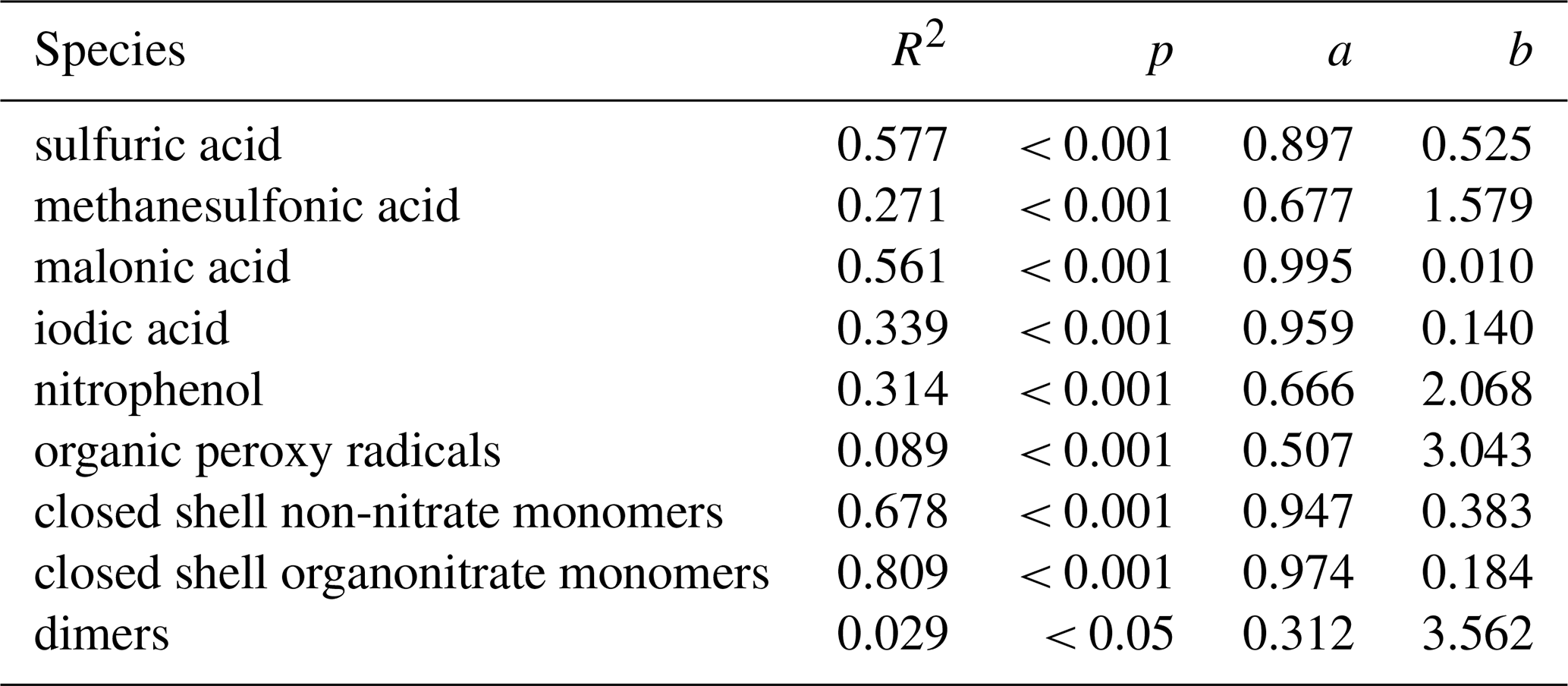
Table 7 summarizes the results of the correlation analysis for the species targeted in NO${}_{\mathrm{3}}^{-}$ mode. Overall, the instruments show moderate agreement for sulfuric acid, poor to moderate agreement for the selected HA species, and moderate to good agreement for closed shell HOM monomers, including both non-nitrate and organonitrate species. In contrast, agreement is poor for the remaining HOM monomer class, namely organic peroxy radicals, as well as for HOM dimers. However, the low coefficient of determination for the former is largely driven by the behavior of EH1 (Fig. S4 in the Supplement). For HOM dimers, the poor agreement mainly reflects the clear separation between instruments between the behavior of instruments with Eisele-type inlets and with MION inlets. Finally, the reason for the poor agreement observed for HAs could not be clearly identified. Additional correlation analysis tables are presented in Sect. S12 in the Supplement.

3.4 Measurements in bromide mode

Similar to Figs. 4 and 5 in Sect. 3.3, Fig. 6 shows the concentrations of different species detected using bromide as the reagent ion, comparing ML1 and ML2. Specifically, the analysis focuses on SVOCs (Table S3), for which Br⁻ is more selective towards, and the HOM class of closed shell non-nitrate monomers ($m/z$ 308–374; Table S3), which are expected to cluster less efficiently with Br⁻ compared to NO${}_{\mathrm{3}}^{-}$ (see Sect. 2.2.5).

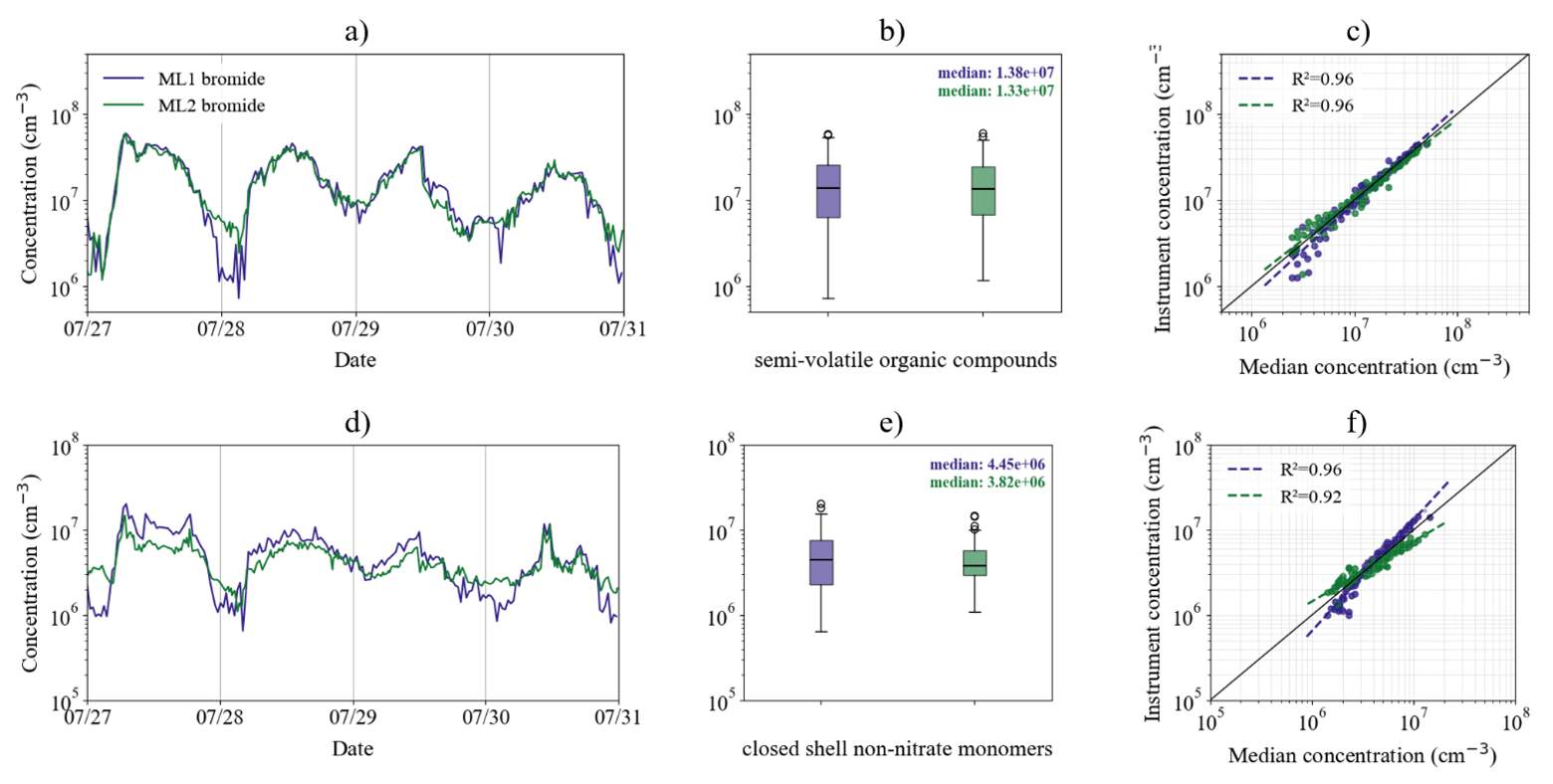
Figure 6 Concentrations of (a–c) semi-volatile organic compounds, and (d–f) closed shell non-nitrate monomers measured in bromide mode by ML1 and ML2 during 27–30 July 2024. For each panel, the left panels (a, d) show concentration time series, while the central panels (b, e) show a box plot summarizing the distributions over the same period. Boxes indicate the interquartile range, horizontal lines indicate the median, whiskers represent the non-outlier range, and empty circles denote outliers. The right panels (c, f) show the hourly median concentration measured by each instrument against the mean of the corresponding hourly median concentrations from the two instruments. Dashed lines indicate log–log linear regressions for each instrument, with the corresponding coefficient of determination (R²) reported in the legend. Outliers are plotted as smaller semi-transparent points and are excluded from the linear fits.

The top panel of Fig. 6 shows that the two instruments are in good agreement (R² = 0.853; see Table S11 in the Supplement) for most of the time when measuring SVOCs. In contrast, larger discrepancies exist for species that bind less efficiently to Br⁻, such as the selected closed shell non-nitrate monomers. This is illustrated in the bottom panel of Fig. 6, where noticeable differences are observed both at low and at high concentrations. With the settings used in the ACTRIS CI-FI1 campaign, ML1 appears to more effectively resolve both the lowest and the peak concentrations for these species. Despite these differences, the overall performance in bromide mode is encouraging. As reported in previous studies (He et al., 2023; Hyttinen et al., 2018), the RH conditions during the campaign (39 %–100 %; see Sect. 2.1) were not optimal for operating in Br⁻ mode, since the detection sensitivity decreases noticeably at RH above approximately 20 %–40 %, with the effect expected to be stronger for compounds forming less stable clusters with the reagent ion. Nevertheless, for species that are typically targeted using Br⁻, the two instruments show consistent behavior, suggesting that bromide-mode measurements may remain robust under field conditions and may be less susceptible to variations in ambient moisture than previously anticipated. However, it cannot be excluded that ML1 and ML2 were similarly affected by the variations in RH, and this possibility is further considered in the following section by comparing the Br⁻ and NO${}_{\mathrm{3}}^{-}$ measurements.

3.5 Measurements in different reagent ion modes: nitrate, bromide, and iodide

Having an instrument measure in multiple reagent ion modes can be useful for identifying issues affecting the individual modes. Accordingly, since two instruments were operated in both NO${}_{\mathrm{3}}^{-}$ and Br⁻ mode, we investigated whether the response toward selected compounds varied consistently with reagent ion choice in the two instruments. During ambient sampling side by side, ML1 and ML2 switched every 10 min among NO${}_{\mathrm{3}}^{-}$ ionization, Br⁻ ionization and non-ionizing mode; in this way, both instruments and each ionization mode were exposed to the same analyte concentrations under identical ambient conditions.

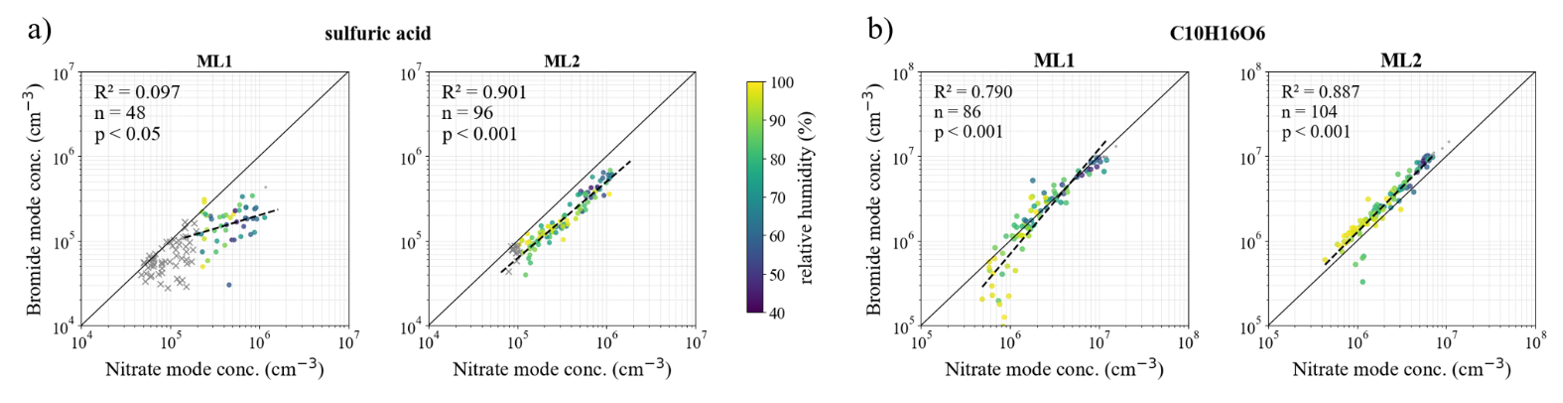
Figure 7 Scatter plots of hourly median concentrations measured in bromide mode versus nitrate mode for (a) sulfuric acid and (b) C₁₀H₁₆O₆ obtained with ML1 and ML2 during 27–30 July 2024. Dashed lines indicate linear regressions for each plot, with the corresponding coefficient of determination (R²), number of data points considered (n), and probability value (p) reported. The color of the points represents the relative humidity, as indicated by the color bar in the center. Points falling below the corresponding LOD_CIMS are shown as crosses (X), while outliers are plotted as smaller semi-transparent points; both are excluded from the linear fits.

In Fig. 7, we selected two compounds for which both reagent ions are selective (see Sect. 2.2.5), namely sulfuric acid and the SVOC C₁₀H₁₆O₆, and plotted the concentrations measured in Br⁻ mode against those measured in NO${}_{\mathrm{3}}^{-}$ mode for the two instruments. The figure highlights some differences in behavior between the instruments. For ML2, the high R² values in both cases suggest good agreement between the two ionization modes in detecting the selected species over a wide concentration range. The distribution of the data points further indicates that, as expected, NO${}_{\mathrm{3}}^{-}$ is more sensitive to sulfuric acid than Br⁻, whereas the opposite behavior is observed for C₁₀H₁₆O₆, with which Br⁻ forms more stable clusters than NO${}_{\mathrm{3}}^{-}$ does (Hyttinen et al., 2018). The RH bars in all panels further suggest that RH does not play a major role in driving the performance of Br⁻ mode relative to NO${}_{\mathrm{3}}^{-}$ mode, despite the reduced Br⁻ sensitivity expected under the elevated RH experienced during the measurements, further supporting the interpretation proposed in the previous section. For ML1, however, the lower R² values and the larger dispersion of the data points indicate greater discrepancies in the detection of sulfuric acid at different concentration levels. In part, this behavior likely owes to the substantial fraction of the Br⁻ mode measurements falling close to or below the detection limit for ML1. In addition, peak fitting for sulfuric acid may be more challenging in Br⁻ mode than in NO${}_{\mathrm{3}}^{-}$ mode, since the HSO${}_{\mathrm{4}}^{-}$ peak ($m/z$ 96.960) nearly overlaps with the Br⁻ water cluster, (H₂O) ⋅ Br⁻ ($m/z$ 96.929). The fact that such a discrepancy is not observed for ML2 does not exclude the possibility that peak overlap affected ML1 more strongly, since different instrument settings may lead to different fragmentation of Br⁻ water clusters, which can affect the intensity of (H₂O) ⋅ Br⁻ and its separation from HSO${}_{\mathrm{4}}^{-}$, making the sulfuric acid peak more difficult to fit in ML1.

These results indicate that the relative performance of the two ionization modes cannot be explained solely by reagent ion chemistry and that it is also strongly instrument-dependent. In particular, the different behavior observed for ML1 and ML2 suggests that differences in instrument settings and other operating conditions may contribute substantially to the observed differences not only among the Br⁻ measurement themselves, but also in comparison to the NO${}_{\mathrm{3}}^{-}$ measurement.

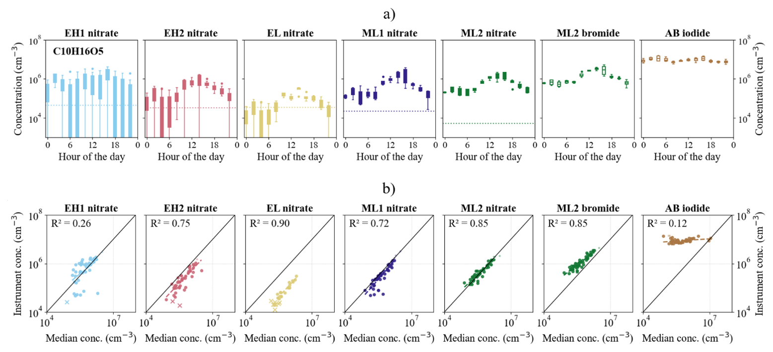
Figure 8 (a) Box plots showing the diurnal variation of C₁₀H₁₆O₅ based on measurements conducted on 1–2 August 2024. Data are from five instruments operating in nitrate mode (EH1, EH2, EL, ML1, ML2), one instrument operating in bromide mode (ML2), and one instrument operating in iodide mode (AB). Boxes indicate the interquartile range, whiskers represent the non-outlier range, and full circles denote outliers. For the instruments operating in nitrate mode, instrument-specific LOD_CIMS values are indicated by dotted horizontal lines. (b) Scatter plots of hourly median concentrations showing, for each instrument and ionization mode combination, the concentrations measured by the individual instrument-mode against the median concentration measured across all instruments-mode combinations over the same period. Dashed lines indicate linear regressions for each instrument, with the corresponding coefficient of determination (R²) reported in the figure.

Finally, to further investigate how the response toward selected compounds varies with both instrument and reagent ion, we took advantage of the fact that AB also operated in I⁻ mode and selected a few SVOCs that were expected to be detectable, at least to some extent, by all three reagent ions (NO${}_{\mathrm{3}}^{-}$, Br⁻, and I⁻). This provided an opportunity to compare all instruments participating in the ACTRIS CI-FI1 campaign. Figure 8a shows the diurnal variation of C₁₀H₁₆O₅, while Fig. 8b presents the hourly median concentrations measured by each instrument and ionization mode plotted against the median of the hourly median concentrations measured by all of them. We note that this species, containing only five oxygen atoms, is not expected to be detected with full sensitivity with NO${}_{\mathrm{3}}^{-}$ (see Sect. 2.2.5); nevertheless, it was selected because it represents one of the most oxygenated compounds that could be detected by all six instruments in the three ionization modes of interest. Additional species are shown in Sect. S15 in the Supplement.

As predicted, in NO${}_{\mathrm{3}}^{-}$ mode, instruments with an Eisele-type inlet do not detect C₁₀H₁₆O₅ with optimal sensitivity, especially in the case of EH1, for which the corresponding peak is not clearly distinguishable from the background noise signal. Similarly, for EH2 and EL, the signal is close to or below the detection limit. However, the two instruments with MION inlets can resolve the peak more clearly over the daily concentration range also in this ionization mode, and they show similar behavior. ML2 operating in Br⁻ mode, which is expected to be the configuration best suited for detecting this species, shows a response very close to the NO${}_{\mathrm{3}}^{-}$ mode measurements from ML1 and ML2. By comparison, under the present sampling conditions and instrument configuration, I⁻ mode showed substantially poorer agreement with the other instruments and a limited ability to resolve variations in C₁₀H₁₆O₅ concentrations. This behavior is not unexpected, given the fundamental differences in operating pressure of the inlet between the bipolar instrument and the other mass spectrometers and, consequently, the higher LOD expected for AB. The substantial difference between this instrument and the others may also contribute to the overall higher concentrations reported by AB, although other factors, such as differences in data processing and concentration calculation, may also play a role. In this regard, for the purpose of the intercomparison, the different response of AB to variations in C₁₀H₁₆O₅ concentrations is more relevant than the difference in absolute concentration.

Overall, instruments with the same inlet configuration behave more similarly to each other compared to instruments using the same reagent ion. In particular, the way EH1, EH2, and EL detect C₁₀H₁₆O₅ can be clearly distinguished from the behavior of ML1 and ML2, both in NO${}_{\mathrm{3}}^{-}$ and Br⁻ mode. Likewise, the different behavior observed in I⁻ mode appears to be more strongly related to the substantially different instrument configuration employed in this mode than to the reagent ion type itself, which would be expected to detect a compound containing five oxygen atoms in a manner broadly comparable to NO${}_{\mathrm{3}}^{-}$ (Hyttinen et al., 2018; Riva et al., 2019, 2024). These results further confirm that reagent ion choice is not the only important factor determining selectivity toward selected compounds; instrument configuration, here primarily the inlet design and its operating pressure, also plays a defining role.

4 Conclusions

Understanding the formation and growth of new atmospheric particles requires accurate measurements of key condensable vapors, including sulfuric acid and highly oxygenated organic molecules. Chemical ionization mass spectrometry has proven to be well suited for this purpose; however, the many factors influencing instrument performance pose challenges for achieving consistent and comparable measurements across different studies. Intercomparison campaigns are therefore important for assessing how differences in instrument configuration and operation methods influence the response toward the detection and quantification of selected compounds and, consequently, the agreement among instruments.

In this study, we compared data from six chemical ionization mass spectrometers, some of which operated using multiple reagent ions, resulting in a total of ten measurement modes, of which eight were analyzed in this work. The ambient measurements were conducted at a boreal forest site under rainy conditions, resulting in relatively low measured concentrations that were often close to the instruments' limits of detection. Although these conditions introduced some measurement limitations, the ACTRIS CI-FI1 campaign provided several important insights into the comparability of condensable vapor measurements obtained using different chemical ionization mass spectrometers during field operations.

1. For sulfuric acid measured in nitrate mode, the traditional calibration based on gas-phase sulfuric acid enabled moderate agreement among the participating instruments (R² = 0.577), with the highest consistency observed during daytime concentration maxima. Larger discrepancies occurred at lower concentrations, where the measurements approached the corresponding detection limits.

2. For higher molar-weight compounds, such as highly oxygenated organic molecules, sulfuric acid calibration alone was not sufficient to ensure consistent inter-instrument comparison. The results showed that accounting for mass-dependent transmission differences can substantially improve the agreement for HOM measurements. At the same time, the study demonstrated the importance of critically evaluating whether a derived transmission curve provides a reliable representation of instrument behavior before applying the corresponding correction. In nitrate mode, after applying the corrections discussed in this study, the instruments showed good agreement for closed shell HOM monomers, with R² values of 0.678 and 0.809 for non-nitrate and organonitrate monomers, respectively (0.831 and 0.891 when excluding EH1 from the correlation analysis). In contrast, agreement was poorer for organic peroxy radicals and HOM dimers; the latter showing clear differences between instruments with Eisele-type and MION inlets over the range of concentrations measured.

3. For organic and inorganic acids of relatively low molecular mass (below $m/z$ 250) considered in this study (HAs), the agreement among instruments was generally poorer than for sulfuric acid and HOMs. The reason for these larger differences could not be clearly identified. One possible explanation considered was the lack of correction for relative transmission differences for these species; however, additional analysis showed that applying this correction did not improve the agreement among instruments. The results therefore suggest that the measurement of these compounds remains challenging, and that further work is needed to better understand and improve their quantitative determination by CIMS.

4. The bromide mode comparison yielded encouraging results for the selected SVOCs, for which ML1 and ML2 showed good agreement (R² = 0.853) despite the elevated RH conditions encountered during the campaign. The comparison of nitrate and bromide mode measurements further indicates that the elevated and variable RH conditions did not strongly affect the relative behavior of Br⁻ mode for the selected compounds. These observations suggest that bromide-mode measurements can remain robust under ambient conditions for compounds forming sufficiently stable clusters with Br⁻ ions.

5. Finally, the comparison between nitrate, bromide, and iodide modes demonstrated that, although all instruments showed qualitatively similar diurnal patterns, differences in signal intensity were often more closely associated with instrument configuration than with reagent ion choice itself. Specifically, instruments sharing the same inlet design showed more similar responses toward selected compounds than instruments operating with the same reagent ion but different configurations.

The ACTRIS CI-FI1 campaign proves that (a) comparable measurements of condensable vapors by different CIMS instruments are achievable when all relevant calibration and correction factors are critically applied, and (b) inter-instrument comparability is strongly influenced not only by reagent ion chemistry, but also by inlet design and instrument operating conditions, including operating pressure. At the same time, it is worth acknowledging that, since these instruments are generally not calibrated for every targeted analyte, the use of a common calibration factor for groups of species remains an approximation because the sensitivity of a given reagent ion can vary between them, and the application of additional correction factors can only partially account for these differences, which may contribute to the less consistent agreement observed for some species.

Hence, detailed guidelines on measurement principles and calibration procedures are urgently needed to ensure good comparability and quantification of condensable vapors across different observations, thereby improving our ability to evaluate and interpret new particle formation processes.