Observing formation and early evolution of contrails formed by IAGOS aircraft using high-resolution LEO satellite imagery

Persistent contrails and contrail cirrus are estimated to be a major contributor to the climate impact of aviation. The mitigation of these impacts by means of technological or operational changes benefits from the ability to skillfully model the formation, evolution, and impacts of contrails. Although these models can be evaluated and improved by use of observations of contrails obtained from remote sensing instruments, these comparisons are hindered by uncertainty in the required meteorological data (such as relative humidity) and limitations in the method of observation (such as younger contrails not being observable in geostationary satellite imagery). To address these challenges, we collocate aircraft equipped with in situ humidity sensors from the IAGOS fleet in high-resolution (10–30 m) satellite imagery obtained by instruments aboard the low Earth orbit (LEO) Sentinel-2 and Landsat missions. The resulting dataset consists of 543 IAGOS aircraft found in satellite imagery (51 % of which form contrails), which we use to evaluate predictions of contrail formation by the Schmidt–Appleman criterion (SAC) as well as predictions of contrail growth by the CoCiP model. When accounting for uncertainty in the IAGOS measurements of humidity and temperature, we find that the SAC correctly explains 98.3 % of the observations for the aircraft in the IAGOS fleet. Disagreement between predictions and observation increases when using meteorological data from the ERA5 reanalysis, with only 92.1 % of the observations being explained correctly. Out of the 195 annotated contrails, 48.2 % of these contrails were found to persist for longer than 10 s (approximately the jet phase) and 8.7 % longer than 120 s (approximately the vortex phase). The relative humidity with respect to ice is found to correlate most strongly with observed contrail lifetime, exhibiting an R² value of 0.49 with the logarithm of contrail age. The observed horizontal growth during the jet and vortex phases is consistent with previous observations and contrail model results. Although the limited lifetimes of the annotated contrails prevent robust statistical conclusions for the dispersion phase, three example cases illustrate how the observed horizontal growth can be compared with contrail simulation results. Overall, this study demonstrates the potential of high-resolution LEO satellites to create observational datasets for evaluating and improving models of contrail formation and early evolution.

1 Introduction

Condensation trails, or contrails, are linear clouds formed behind aircraft when hot engine exhaust mixes with the colder, drier ambient air (Schumann, 1996). While most contrails dissipate within minutes, some can persist for several hours when the air is sufficiently humid with respect to ice, eventually turning into cirrus-like clouds (Kärcher, 2018). Contrails affect Earth's energy balance by interacting with incoming solar and outgoing terrestrial radiation, resulting in a net warming effect, with current estimates suggesting that contrails are responsible for over half of aviation's total radiative impact to date, with an effective radiative forcing of 57.4 mW m⁻² for 2018 (Lee et al., 2021), albeit with high uncertainty (17–98 mW m⁻², representing the 90 % confidence interval).

Proposed options for the mitigation of contrail climate impacts include alternative fuels (Burkhardt et al., 2018; Voigt et al., 2021; Märkl et al., 2024) and re-routing aircraft to avoid the regions where persistent, warming contrails can form (Teoh et al., 2020; Martin Frias et al., 2024; Sausen et al., 2024; Sonabend-W et al., 2024). The implementation of such mitigation options is complicated by uncertainties in predictions of where contrails form, persist, and what their impact on the climate is (Petzold et al., 2025).

The uncertainties in these predictions can be assessed, and potentially reduced, by comparing model outputs to observations. These observations can come from in situ measurements or remote sensing. In situ observations can provide detailed information on the microphysics of contrails (Voigt et al., 2010, 2011; Jeßberger et al., 2013; Schumann et al., 2017; Voigt et al., 2021), but are often limited in their spatio-temporal coverage. On the other hand, remote sensing observations can provide larger spatio-temporal coverage but cannot provide information at the level of detail possible by in situ measurements (Mannstein et al., 1999; Meijer et al., 2022; Geraedts et al., 2024). Geostationary satellite images are captured several times an hour and can be used to observe contrails (Meijer et al., 2022; Ng et al., 2023; Ortiz et al., 2025) and estimate their properties over large regions (Chevallier et al., 2023; Gryspeerdt et al., 2024; Meijer et al., 2024; Sarna et al., 2025; Sonabend-W et al., 2026).

The process of comparing these contrail observations to model outputs is complicated by limitations in the model input data and the reliability of observations. For example, numerical weather prediction (NWP) data of relative humidity, which is an important input to contrail models, are known to be unreliable in the upper troposphere (Gierens et al., 2020; Geraedts et al., 2024). Therefore, disagreement between observations and model predictions based on NWP data cannot unambiguously be attributed to errors within the contrail model. Observations themselves can also be affected by errors. For example, the relatively coarse (1–2 km spatial resolution at nadir) geostationary satellite images can miss thinner contrails (Vazquez-Navarro et al., 2010; Driver et al., 2025; Euchenhofer et al., 2025). As a consequence, these images cannot be used to observe the first phases of the lifetime of a given contrail, and other instruments should be used instead, such as those available on the ground and low Earth orbit (LEO) satellites.

Thus, existing approaches for the evaluation of contrail models using observational data are constrained by uncertainty in relevant model input data as well as limitations of the method of observation used. Here, we address these challenges by locating in situ measurement aircraft in high-resolution (10 to 30 m) satellite imagery in order to evaluate models of contrail formation and early evolution while using measurement-based meteorological input data. Specifically, we collocate aircraft from the In-service Aircraft for a Global Observing System (IAGOS) program (Petzold et al., 2015) in satellite imagery from the Sentinel-2 and Landsat missions and compare this to predictions of contrail formation using the Schmidt–Appleman criterion (SAC) (Schumann, 1996) and contrail evolution from the Contrail Cirrus Prediction (CoCiP) model (Schumann, 2012).

The SAC has been evaluated using both in situ and remote sensing observations of contrails, results of which have been summarised in Schumann et al. (2017). Based on 236 datapoints from 33 independent observation campaigns, that study reported that 93.6 % of observed contrails were predicted by the SAC. However, because the dataset comprises only cases in which contrails were actually observed, the analysis could not evaluate situations where the SAC predicted contrail formation but none was observed. Recent ground-based observations that include aircraft both forming and not forming contrails found that SAC predictions based on NWP data correctly predict contrail formation in only 75.8 % of cases (Low et al., 2025), or even fewer (Jarry et al., 2026). One reason for this might be the quality of the weather data. Gierens et al. (2020) investigated the impact of uncertainties in NWP data used for evaluating the SAC and found that NWP data correctly predicts the SAC in 94 % of cases when compared to in situ measurements. However, this study did not take any observations of contrails into account. It thus remains unclear whether the lower agreement between the SAC and observations found by Low et al. (2025) and Jarry et al. (2026) arises from limitations of the observations, uncertainties in the underlying meteorological input data, or the SAC itself.

In situ and remote sensing observations have also been used to investigate contrail properties at different stages of their lifetimes (Iwabuchi et al., 2012; Schumann et al., 2017; Märkl et al., 2024; Low et al., 2025). These studies reported distributions of contrail properties, for example the width, depth, and ice water content, to be consistent with model simulations. Observations of young contrails (jet/vortex phase) are, however, limited, either due to the difficulty of performing measurements in the aircraft wake (Jeßberger et al., 2013) or due to the limited detection capabilities of satellite instruments (Driver et al., 2025; Euchenhofer et al., 2025). LIDAR and ground-based camera studies have the ability to detect young contrails, but are constrained by their limited spatial coverage, restricting observations to the field of view of the site. High-resolution LEO satellites, however, do have the ability to detect contrails at formation, on a global-scale.

Both Sentinel-2 and Landsat have been used to observe aircraft in satellite imagery, for example for airspace management and surveillance (Zhao et al., 2018; Heiselberg, 2019; Liu et al., 2020). Observing contrails has been done in the Landsat (McCloskey et al., 2021) for the purpose of creating human-labelled datasets for evaluating contrail detection algorithms. However, this is done with a contrail-first approach, meaning contrails are annotated not linked to individual flights. Our approach differs in that we first locate the aircraft within the satellite image based on trajectory data, after which we annotate the contrail in case it is formed.

In this paper, we present a methodology for locating IAGOS aircraft in high-resolution Sentinel-2 and Landsat satellite imagery. The approach is used to collect data on contrail formation and early evolution for 543 IAGOS aircraft, 195 of which were found in Sentinel-2 imagery and thus include annotations of the entire observed contrail (in the case one was formed). The resulting dataset is used to evaluate the performance of the SAC in predicting contrail formation and how this is affected by input data quality (using ERA5 instead of IAGOS measurements) and satellite image resolution (by considering Landsat instead of Sentinel-2 collocations). We also compare the observations of contrail growth with corresponding model predictions, and study the relationship between observed contrail lifetimes and measurements of humidity and temperature.

2 Data methodology

2.1 Satellite data

2.1.1 Sentinel-2 data overview

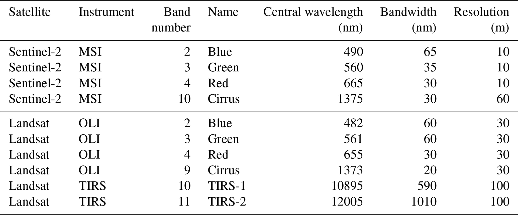
The Sentinel-2 (Drusch et al., 2012) mission is part of Europe's Copernicus program (Berger et al., 2012). During the period relevant to this study (2013–2022), two satellite platforms were operational: the S2A (2015–2025) and the S2B (2017–present). By using the two-satellite constellation, the revisit time is reduced from 10 to 5 d. All Sentinel-2 satellites are in a sun-synchronous orbit at an altitude of approximately 786 km. The Sentinel-2 satellites carry the Multi-Spectral Instrument (MSI) which acquires high spatial resolution (10 to 60 m) imagery in 13 bands in the visible and near-infrared part of the electromagnetic spectrum, with a swath width of 290 km. The four MSI bands used in this study, along with their wavelengths, spatial resolution and what features are visible in them, are given in Table 1. The satellite image data are subdivided on a predefined set of 110 by 110 km tiles defined in the UTM/WGS84 projection. We use L1C data which are downloaded from a public Google Cloud Storage dataset (Google, 2026).

Table 1 Sentinel-2 MSI and Landsat 8/9 OLI and TIRS bands used in this study, along with their specifications.

2.1.2 Landsat 8/9 data overview

The Landsat 8 (2013–present) and Landsat 9 (2021–present) satellites (Irons et al., 2012; Knight and Kvaran, 2014; Masek et al., 2020) are operated by the U.S. Geological Survey (USGS) and the National Aeronautics and Space Administration (NASA). The Landsat 8 and 9, hereafter referred to as Landsat, have a revisit time of 16 d each, or 8 d when using both satellites. Both satellites are in a sun-synchronous orbit at an altitude of 705 km and have a swath width of 185 km. The Landsat carries two instruments: the Operational Land Imager (OLI) and the Thermal Infrared Sensor (TIRS). The spectral bands used, along with their wavelengths and spatial resolution are given in Table 1. We use the Landsat 8 and 9, Collection 2, Level 1 data downloaded from the USGS EROS machine-2-machine API (U.S. Geological Survey, 2026).

2.2 IAGOS fleet and data

The In-service Aircraft for a Global Observing System (IAGOS) (Petzold et al., 2015) operates measuring equipment on commercial aircraft to provide in situ atmospheric measurements on a global scale. The IAGOS dataset, which starts in 1994, consists of the former research project MOZAIC, CARIBIC (now IAGOS-CARIBIC), and the currently active CORE program. In this study, we only considered the aircraft that are part of the CORE program, as shown in Table 4, as these were predominantly active throughout the operational periods of Sentinel-2 and Landsat 8 and 9.

We use the air temperature (T) and the relative humidity w.r.t. liquid (RH_l) from the IAGOS-CORE dataset, both of which are measured by the IAGOS capacitive hygrometer (ICH). The ICH uses a capacitive humidity sensor (a modified Vaisala HUMICAP^® sensor) and a platinum resistance temperature sensor (PT100) (Helten et al., 1998; Neis et al., 2015b). The IAGOS aircraft trajectory data and ICH measurements are provided every 4 s. During this study we observed a time shift in the IAGOS data in the order of 0–15 s when compared to ADS-B data or satellite imagery. To resolve this, we linearly interpolate the IAGOS measurement and position data to a 0.1 s resolution and select the time at which the aircraft position is closest to the annotated aircraft position, when corrected for parallax (see Appendix C4).

IAGOS data undergo quality control, the outcome of which is communicated by means of a validity flag. These flags are either good (0), limited (2), erroneous (3), not validated (4), or missing value (7) (IAGOS, 2026). For this study, only measurements flagged as good (0), for both T and RH_l, were used. This entails that the measurements passed all required quality control tests. In addition to these validity flags, we utilise the estimates of measurement uncertainty that come with IAGOS data for both T and RH_l to construct 95 % confidence intervals. The uncertainty of T and RH_l measurements are estimated to be 0.5 K (Berkes et al., 2017) and 5 %–6 % (Neis et al., 2015b, a) respectively, with the latter determined by comparing the ICH measurements with the FISH (Meyer et al., 2015) and SEALDH-II (Buchholz et al., 2013) instruments during the AIRTOSS-ICE field campaign (Neis et al., 2015b). However, instead of taking this constant T and RH_l uncertainty, we rely on the uncertainty estimates provided directly by the IAGOS data processing. In general, these uncertainties are comparable to the 0.5 K for air temperature and 5 %–6 % for RH_l, but they offer a more accurate representation of the uncertainty associated with individual measurements.

Humidity measurements by the ICH in the upper troposphere and lower stratosphere (i.e. the aircraft cruise altitude region) may also be affected by reduced sensor sensitivity and long sensor response times. Firstly, relative humidity measurements by the ICH have been reported to suffer from reduced sensitivity to water vapour concentrations in dry stratospheric air masses (Kunz et al., 2008; Rolf et al., 2024), with a lower detection limit between 10 ppmv (Engel et al., 2006) and 30 ppmv (Rolf et al., 2024). This loss of sensitivity is primarily caused by adiabatic heating of the air flow, as it is brought to rest within the ICH housing. Because of this temperature increase, the measured RH_l is lower than the ambient RH_l. The effect of this lower detection limit on the analysis conducted in this study will be further discussed in Sect. 2.5. Secondly, the humidity sensor has a temperature-dependent response time, which varies from 1 s at 300 K to 120 s at 210 K. Several studies have attempted to correct this time delay or mitigate its effects on downstream analysis. For example, Gierens et al. (2007) aggregates measurements to a coarser 1 min resolution, whereas Borella et al. (2024) tries to reconstruct the measured signal by use of a temperature-dependent exponential moving average. We find that reconstructing RH_l for the IAGOS flights at 4 s timestamps results in a noisy signal (on average increasing the first-difference (i.e., the difference between successive samples) standard deviation by 43.3 %), resulting in more outlier measurements. Resampling to 1 min timestamps mitigates this noise, but does so at the expense of temporal resolution. Therefore, we chose not to apply any of the aforementioned correction methods.

2.3 Numerical weather prediction data

We use numerical weather prediction (NWP) data from the ECMWF ERA5 reanalysis dataset (Hersbach et al., 2020). Air temperature (T), specific humidity (q) and pressure (p) are used to compute RH_l and RH_i with the expressions for the saturation pressure w.r.t. liquid from Buck (1981) and ice from Alduchov and Eskridge (1996). Other variables required to use the CoCiP contrail model (Schumann, 2012) also come from the ERA5 dataset. The reanalysis data are downloaded from the Analysis-Ready, Cloud Optimized (ARCO) ERA5 Dataset (Carver and Merose, 2023) hosted on Google Cloud, which has a regular grid of 0.25°×0.25° horizontal resolution and includes 137 vertical model levels extending from the surface to approximately 80 km. The air temperature and relative humidity are linearly interpolated in the horizontal and vertical dimensions to match the aircraft's position and time.

2.4 Aircraft performance modelling

We use two aircraft performance models (APMs) to estimate the engine fuel mass flow and the overall propulsion efficiency which are required as inputs for modelling contrail formation and evolution: the Base of Aircraft Data (BADA) Family 4 Release 4.2 (EUROCONTROL, 2016) and the Poll–Schumann (PS) (Poll and Schumann, 2021a, b, 2025) model. The aircraft type and engine combinations for the IAGOS fleet are given in Table 4. All computations were performed using the open-source pycontrails library (Shapiro et al., 2026). Flight trajectories provided by IAGOS at 4 s resolution were resampled to 1 min, in order to reduce the influence of small positional uncertainties and obtain smoother overall propulsion efficiency outputs. Both APMs require data on air temperature and horizontal winds as input, which can either come from ERA5 or the IAGOS measurements. We have quantified the changes in overall propulsion efficiency estimated by both APMs when using these different meteorological data sources: the resulting root-mean square “error” was found to be close to 0.005 for the PS model, and 0.009 for the BADA 4.2 model, which is almost 2 orders of magnitude smaller than typical propulsion efficiency values of 0.3–0.4. Due to the relatively small magnitude of these meteorology-dependent efficiency differences, we have chosen to perform aircraft performance calculations with the data source that is used for the prediction of contrail formation, which we discuss in more detail in Sect. 2.5.

Comparison of the two APMs shows that BADA 4.2 propulsion efficiencies show larger intra-flight variability than those obtained from the PS model. As a result, the efficiency values calculated for the satellite observation times also show increased variability, typically ranging between 0.2 and 0.4 during cruise, as opposed to 0.25 to 0.35 with the PS model. Moreover, during descent, BADA 4.2 calculates an overall propulsion efficiency of zero, whereas the PS model calculates values between 0.1 and 0.3. For the subsequent analyses, we therefore only use the PS propulsion efficiency estimates. Additional details and a comparison of the two performance models are provided in Appendix A3.

In the PS model, the overall propulsion efficiency at the optimum condition is expected to have an uncertainty of no more than ±10 % (Poll and Schumann, 2021b). Since this uncertainty is related to the optimum condition, an extra 2.5 % buffer is added to account for suboptimal conditions. In the updated version (Poll and Schumann, 2025), an extra uncertainty of ±2.5 % is added due to the effect of in-service engine deterioration, based on the reasoning that an airline only allows for an increase of 5 % in fuel consumption before a maintenance intervention is planned. Thus, we take an uncertainty related to the overall propulsion efficiency of 15 % into consideration for the subsequent analyses. For example, for an efficiency of 0.3, we take the confidence interval as [0.255, 0.345]. We note that this constant 15 % uncertainty does not take into account local flight conditions and can mask local thrust variations.

2.5 Contrail models

2.5.1 Schmidt–Appleman criterion

Contrails form when water condenses onto particles in the engine exhaust plume. For this condensation to occur, the engine exhaust plume is required to be supersaturated with respect to liquid for some period of time during the mixing process with the ambient air. The Schmidt–Appleman criterion (SAC) (Schumann, 1996) can be used to ascertain whether this supersaturation occurs, by modelling the mixing of the engine exhaust with the ambient air as an isobaric process. As a consequence, the mixing process can be represented by a straight line in a chart of temperature versus water vapour partial pressure (e) which connects the ambient air state with the state of the engine exhaust. When this “mixing line” is plotted in conjunction with curves representing the saturation pressure w.r.t. liquid (e_l) and ice (e_i), the SAC can be visually confirmed by checking whether the mixing line ever lies above the curve corresponding to e_l. Schumann (1996) has derived an expression for the slope of the mixing line (G, in Pa K⁻¹) as a function of engine, fuel and atmospheric parameters

$$\begin{array}{}\text{(1)}& G={\displaystyle \frac{c_{p}p}{\mathit{\epsilon }}}{\displaystyle \frac{{\mathrm{EI}}_{{\mathrm{H}}_{\mathrm{2}}\mathrm{O}}}{\mathrm{LHV}(\mathrm{1}-\mathit{\eta })}}.\end{array}$$

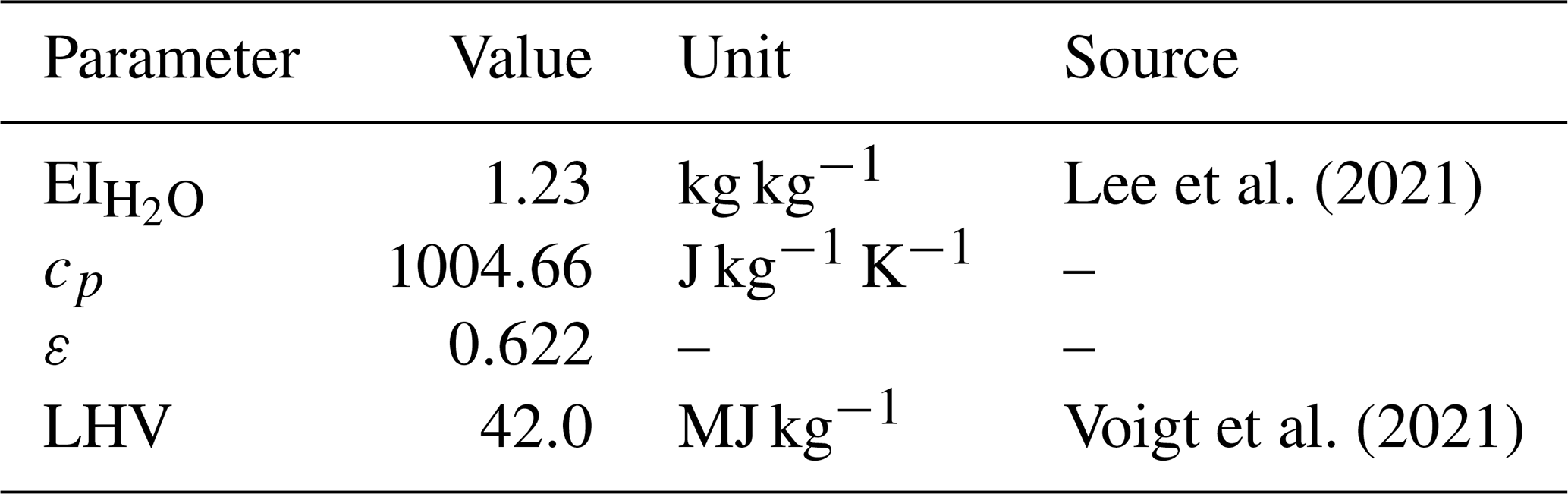
Here, ${\mathrm{EI}}_{{\mathrm{H}}_{\mathrm{2}}\mathrm{O}}$ is the emission index of water vapour associated with combustion of the jet A-1 fuel, c_p is the heat capacity of air at constant pressure, p is the ambient pressure, ε is the ratio of the molar mass of water vapour to that of dry air, LHV is the lower heating value of the fuel, and η is the overall propulsion efficiency. The values used for all these parameters, with exception of p and η (which vary), are given in Table 2.

Lee et al. (2021)Voigt et al. (2021)

Table 2 Values and sources of the fixed parameters used in the mixing slope.

Given the slope G and the ambient temperature and partial pressure of water vapour, we are able to plot the mixing line and ascertain whether a contrail can form. An alternative approach is to, given the slope G, determine the range of ambient conditions for which contrail formation is possible or not. This involves drawing a “limiting mixing line” which is tangent to the curve of saturation pressure w.r.t. liquid. The point of tangency, corresponding to temperature T_LM, is defined by

$$\begin{array}{}\text{(2)}& {\displaystyle \frac{\mathrm{d}{e}_{\mathrm{l}}\left(T_{\mathrm{LM}}\right)}{\mathrm{d}T}}=G.\end{array}$$

Generally, the functional form of e_l(T) prohibits an analytical solution for T_LM. Instead, we use the approximation for T_LM given by Schumann (1996)

$$\begin{array}{}\text{(3)}& \begin{array}{rl}{T}_{\mathrm{LM}}=& -\mathrm{46.46}+\mathrm{9.43}\ln (G-\mathrm{0.053})\\ & +\mathrm{0.720}\left[\ln \right(G-\mathrm{0.053}){]}^{\mathrm{2}},\end{array}\end{array}$$

where T_LM is in °C and G is in Pa K⁻¹. Given G and T_LM, it is possible to determine whether certain ambient conditions allow for contrails to form or not. In order to quantify how “close” particular ambient conditions (in this case T and RH_l) are to the threshold of contrail formation, we also quantify the temperature at which the same RH_l would lead to such threshold conditions. This temperature, denoted as T_LC, is found by solving

$$\begin{array}{}\text{(4)}& T_{\mathrm{LC}}=T_{\mathrm{LM}}-{\displaystyle \frac{e_{\mathrm{l}}\left(T_{\mathrm{LM}}\right)-{\mathrm{RH}}_{\mathrm{l}}{e}_{\mathrm{l}}\left(T_{\mathrm{LC}}\right)}{G}},\end{array}$$

which is done numerically by use of Newton's method. Finally, the difference between this temperature and the ambient one is computed

$$\begin{array}{}\text{(5)}& \mathrm{\Delta }{T}_{\mathrm{LC}}=T-T_{\mathrm{LC}}.\end{array}$$

When ΔT_LC<0, the SAC is satisfied and contrails form.

As mentioned in Sect. 2.2, the IAGOS ICH sensor has a lower detection limit (in terms of water vapour mixing ratio) between 10 and 30 ppmv. At temperatures below 215 K, ice supersaturation (RH_i>1) can occur at these water vapour mixing ratios (e.g. at 250 hPa a measurement at the upper detection limit of 30 ppmv corresponds to RH_i of 0.54 at 215 K, but to RH_i of 1.07 at 210 K). Although the SAC depends on aircraft/engine parameters (e.g. η) and ambient conditions (p, T, and RH_l), it is usually already satisfied in completely dry air for temperatures below 215 K, meaning that inaccurate RH_l measurements will not affect the outcome of the SAC. In the temperature range 215 to 230 K, the slow time response can cause inaccurate measurements of RH_l. Given that the air temperature can be still measured with an uncertainty of 0.5 K and the fact that the satisfaction of the SAC is predominantly influenced by the temperature (Gierens et al., 2020), the slow time response of the humidity sensor is not expected to strongly affect the results. Nevertheless, we will take into account these and other uncertainties in our evaluation.

2.5.2 Contrail Cirrus Prediction Tool (CoCiP)

The Contrail Cirrus Prediction Tool (CoCiP) (Schumann, 2012) is a Lagrangian Gaussian plume model that simulates the full contrail life-cycle. CoCiP does not explicitly model the evolution of the contrail dimensions in the jet and vortex phase. It uses a parametric model to estimate the initial width, depth, and downward displacement that are used to initialise the dispersion phase. This initial width of the contrail is thus the width at the end of the wake vortex phase, which takes place approximately 120 s after formation (Hoshizaki et al., 1972), and is given by (Schumann, 2012)

$$\begin{array}{}\text{(6)}& B_{\mathrm{1}}={\displaystyle \frac{N_{\mathrm{dil}}\left(t_{\mathrm{0}}\right){\dot{m}}_F}{(\mathit{\pi }/\mathrm{4})\mathit{\rho }{D}_{\mathrm{1}}}},\end{array}$$

where N_dil(t₀) is the dilution factor at the effective time scale t₀, with $t_{\mathrm{0}}=\mathrm{2}\mathit{\pi }{b}_{\mathrm{0}}^{\mathrm{2}}/{\mathrm{\Gamma }}_{\mathrm{0}}$, corresponding to the time it takes the vortex pair to descend a distance b₀ at its initial descent velocity; ${\dot{m}}_F$ is the mass fuel flow per flight distance in kg m⁻¹; ρ the ambient air density in kg m⁻³; and D₁ the initial depth in m, which is a function of the maximum downward displacement z_w. This maximum downward displacement is a function of the wake vortex separation, b₀, initial circulation, Γ₀, and the Brunt–Väisälä frequency N_BV.

The lifetime of a contrail in CoCiP is determined by the time at which the contrail segment has fully sublimated. In CoCiP, sublimation is assumed to occur when either the ice particle number concentration drops below 10³ m⁻³ or the optical depth falls below 10⁻⁶.

We use the CoCiP implementation from pycontrails (Shapiro et al., 2026). Flight trajectory data were obtained from IAGOS and resampled to a temporal resolution of 1 s, instead of the default 4 s. Because LEO satellites typically observe only a short segment of an individual contrail (because it is limited by the swath width of the satellite), simulations were run for a maximum contrail age of 20 min with 1 s time steps. The scanning time of the satellite was rounded to the nearest second, such that the contrail dimensions at the scanning time of the satellite could be extracted for each waypoint.

The meteorological input data used to run CoCiP are obtained from ERA5. However, the relative humidity w.r.t. ice (RH_i) in ERA5 shows disagreement with in situ measurements (Gierens et al., 2020). Several approaches exist to correct ERA5 RH_i for contrail modelling, typically by applying correction factors derived from aggregate statistics of IAGOS observations (Teoh et al., 2022, 2024), or using machine learning methods to improve the NWP data (Wang et al., 2025). In this study, in situ IAGOS RH_i measurements are available, allowing for a more accurate, local correction. The ERA5 RH_i values used by CoCiP are adjusted by scaling each value with a factor equal to the ratio of the IAGOS RH_i and the ERA5 RH_i at the scanning time of the satellite.

2.6 Collocation of aircraft in LEO satellite imagery

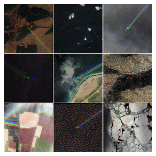
We use aircraft position data (either from IAGOS data or by use of ADS-B data) in combination with satellite ephemeris and imaging sensor specifications to estimate if and where a given aircraft should be located in a particular satellite image: this process is referred to as “collocation”. We find that interpolation of aircraft position data to the image capture time and converting this to the local UTM coordinate system used within the image, leads to differences between the predicted and observed aircraft position on the order of several kilometers. Given that two or more aircraft are occasionally found within a distance of a few kilometers in these images, we apply several corrections to the collocation process in order to resolve such ambiguities. Specifically, we improve the accuracy of the collocation process by accounting for parallax displacement of the aircraft and by using a more precise image capture or “scan” time corresponding to the specific area of the image where the aircraft is expected to be located.

The images are orthorectified to the Earth's surface during Landsat and Sentinel-2 processing, meaning that pixels are geometrically corrected assuming they lie at ground level. While this correction ensures accurate positions for surface features, it introduces a parallax displacement for objects located above the surface of the Earth when they are captured by the instrument at an off-nadir angle. Given the viewing geometry (represented by zenith and azimuth angles) of the satellite instrument and the altitude of the object, this parallax displacement, typically on the order of 1 to 2 km, can be estimated. These viewing angles are provided for each image pixel in the Landsat image metadata, whereas the Sentinel-2 imagery only provides a coarse resolution (25 × 25 km) estimate. We have created an algorithm to correctly upsample the Sentinel-2 viewing angle data which takes into account the staggered architecture of the sensors in the Sentinel-2 MSI (see Fig. 1). This algorithm is described in Appendix C. The geometric (GNSS) altitude of the aircraft, with respect to sea-level (WGS-84), is obtained from the aircraft position data.

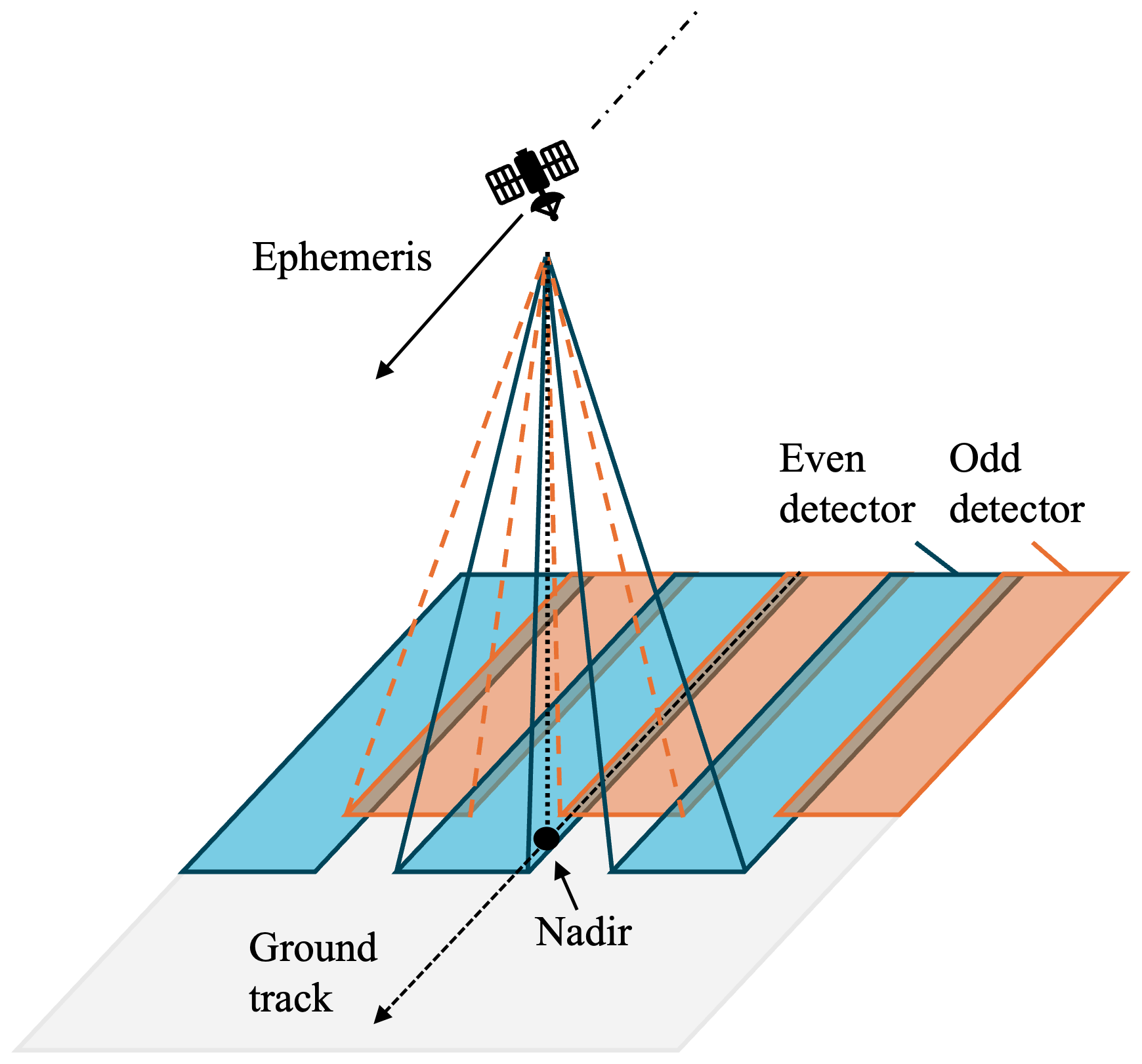
Figure 1 Diagram of scanning time discontinuity due to detector architecture in sensing instrument (note that only 6 detectors are shown of the total 14 detectors in Landsat and 12 detectors in Sentinel-2). Odd detectors (orange) are rear-facing, even detectors (blue) are forward-facing. There is a small overlap between the detectors.

The second correction involves the estimation of the time at which individual image pixels were scanned. Although each satellite image is given a single “sensing time”, this corresponds to the pixel scan time averaged over the entire scene. In practice, scanning such a scene (110 km by 110 km for Sentinel-2 and 170 km by 185 km for Landsat) takes approximately 16.8 s for the Sentinel-2 instrument and 32 s for the Landsat instrument, during which an aircraft cruising at 250 m s⁻¹ can move 4.2 and 7.6 km, respectively. For this reason, it is important to obtain a pixel-by-pixel estimate of the scan time. Both the Landsat and Sentinel-2 imagers are push-broom scanners, but their staggered sensor architecture implies that the pixel scan time is not only a function of the along-track position (as one would expect for a push-broom scanner) but also a function of the cross-track position (determining whether the pixel is scanned by an odd or an even detector). To account for this, we first find the satellite ephemeris position (and the corresponding time) closest to a given pixel, and then apply a constant time offset that depends on the detector used to capture the pixel. Further details on this process can be found in Appendix C.

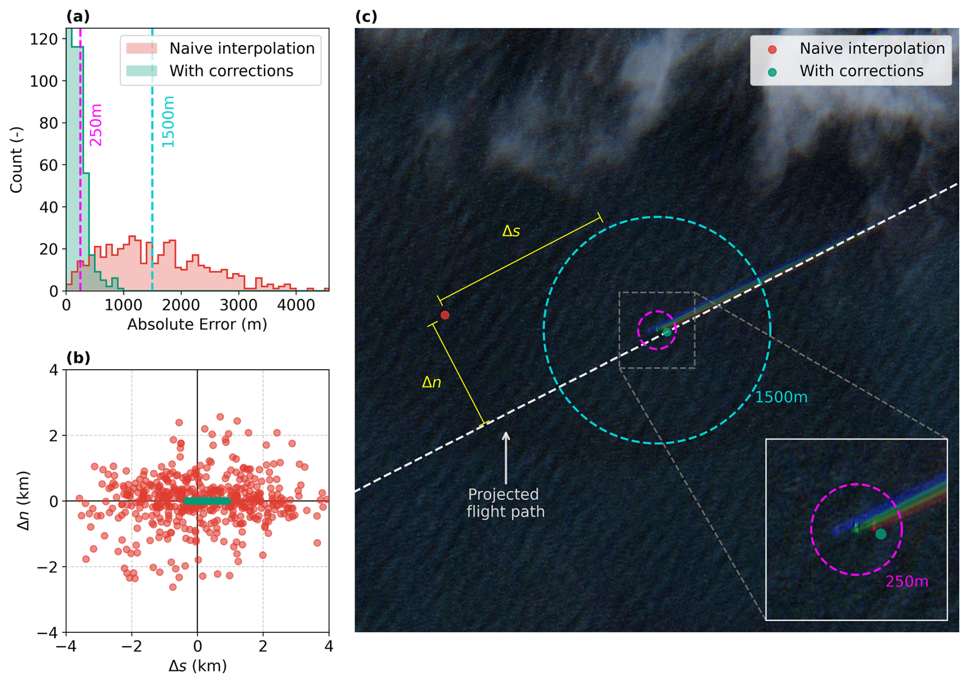
Figure 2 (a) Histogram of collocation errors for naive interpolation (red) and after scanning time and parallax corrections (green). The two vertical dotted lines indicate reference errors for 250 m (magenta) and 1500 m (cyan). (b) Scatterplot showing the errors normal, Δn, and tangential, Δs, to the flight path from the predicted positions to the manually annotated locations. (c) Sentinel-2 true colour image with the PH-TFM (Boeing 787-8 Dreamliner) aircraft, with the 250 and 1500 m reference errors. Collocation for naive interpolation (red) and after corrections (green) shown with the Δn and Δs errors (yellow). Contains modified Copernicus Sentinel data 2022.

The results of these corrections to the collocation process are evaluated by quantifying the distance between the predicted aircraft position and the manually annotated position of the aircraft in the satellite image, and are shown in Fig. 2 for the Sentinel-2. The collocation errors for Landsat are shown in Appendix C. We decompose the error into components normal and tangential to the flight path. As shown in Fig. 2b, the residual error after applying the corrections is predominantly tangential to the flight path. To help interpret the magnitude of the error statistics shown in Fig. 2a–b, we show an example of an aircraft found in a Sentinel-2 image in Fig. 2c along with the predicted aircraft positions with and without corrections. The corrected collocation process estimates the position of 95 % of the aircraft to within a distance of 487 m, whereas the process without the discussed corrections can only narrow down the aircraft position to 3.06 km (for 95 % of the data). This constitutes an order of magnitude improvement in the accuracy of the collocation process.

We hypothesise that the residual errors in the collocated positions are due to: ADS-B timestamp and positional uncertainties (typically in the order of several tens of meters according to Schäfer and Jonáš, 2025), the omission of digital elevation models (which are used in Sentinel-2 (Copernicus, 2024) and Landsat (Franks et al., 2020) processing) in the collocation algorithm, and optical distortions due to the lens composition (Binet et al., 2022).

2.7 Annotation of contrails formed by collocated aircraft

The collocation process described in Sect. 2.6 is used to find the location of IAGOS aircraft within both Sentinel-2 and Landsat imagery, after which we manually identify whether the aircraft in question is forming a contrail. If a contrail is found, it is annotated either by use of a (multi)polygon (for Sentinel-2 imagery) or a linestring along the longitudinal axis of the contrail (for Landsat imagery). As this step is done manually, there might be non-reproducible biases in the placement of the contrail edges, and thus the derived contrail widths. This is particularly relevant for older, more diffuse contrails, where the contrail edges become less distinct from the background.

The first step in this annotation process is to determine the exact location of the aircraft, which is typically found close to but not exactly at the collocated position. In 12 % of cases, out of the total number of cases where an intersection is found between the IAGOS trajectory and the satellite tiles, the aircraft was found to be obscured by clouds or the trajectory data was incomplete. These cases are excluded from the analysis. The second step is to determine whether the aircraft – in case it is visible in the imagery – is forming a contrail. If this is indeed the case, we also annotate the outline (centerline) of the contrail within Sentinel-2 (Landsat) imagery using a polygon (linestring).

For annotating the Sentinel-2 imagery we use the Copernicus Browser (Copernicus, 2026), an ESA platform for visualising satellite data. This tool automatically mosaics adjacent images, enabling contrails to be annotated continuously across the full Sentinel-2 swath width of approximately 290 km. The contrails were manually outlined by the authors as polygon features following their visible extent in the green band, which offers 10 m spatial resolution and generally the highest contrast against the background; the blue band appears less bright over clouds or ocean background, while the red band is less bright over land. Additional bands, including the red, blue, and cirrus bands, were used as aid during the annotation process. The cirrus band was especially useful for long-lived contrails or contrails present above white or “noisy” surfaces (e.g. snowy mountains, salt plains, or cities). In Appendix D, we show four example contrails over clouds, an ocean, a forest, and an urban area (see Fig. D1). In addition, we include two cases in which the contrail is visible either only in the true-colour image or only in the cirrus band (see Fig. D2).

For annotating the contrails found within Landsat imagery: we download the relevant scenes (a scene covers an area of 170 by 185 km) and process these to obtain zoomed images centered on the collocated aircraft position (covering an area of 8 by 8 km). In each case, we computed three images: a true colour image, a monochromatic image from the cirrus band, and a false colour image from the thermal bands (B10 and B11), following the colour scheme from McCloskey et al. (2021). The cirrus band was used for annotating the contrail, with the help of other true colour and false colour images where necessary. Figure D4 shows an example of a contrail as seen in the true colour image, cirrus band, and false colour image.

Because we annotate on zoomed images in Landsat, and we thus have no information on the full lifetime of these contrails, we will not use these cases for determining metrics such as contrail age and width evolution. In Sentinel-2 imagery, a fraction of annotated contrails extends beyond the swath: implying that we cannot see the full extent of the contrail. Such annotations are flagged accordingly to avoid potential misinterpretation.

The Sentinel-2 contrail annotations are further processed to obtain estimates of the contrail width as a function of its age. To estimate the centerline of a polygon, we first compute its minimum rotated rectangle (MRR). When multiple polygons are present, as is the case when the contrail crosses the detector borders, each polygon is processed individually. Then, we compute the longest edge of the MRR and its centroid to construct a centerline along the longest axis. We place points along the polygon centerline spaced by 100 m and estimate the contrail width at these points by computing the width of the polygon orthogonal to the centerline. The age of a contrail at each point (along the centerline) is determined by first calculating the distance from that point to the location of the aircraft. This distance is then divided by the aircraft's groundspeed to estimate the contrail age. The main limitation of this method is that it does not account for horizontal advection of the contrail by the wind. For instance, if the horizontal wind vector is aligned with the direction of flight, a point located 1000 m from the aircraft may have been advected further downstream or upstream. Assuming a wind speed of 50 m s⁻¹ and an aircraft groundspeed of 250 m s⁻¹, this can lead to an error in contrail age of approximately 20 %. Alternative methods, such as generating centerline points by advecting the flight path according to wind, are limited by the accumulation of wind speed errors: over time, these errors can cause the advected path to diverge from the actual contrail. As a result, measurements of contrail width may be taken at an angle that is not perpendicular to the contrail, leading to an overestimation of its width. Thus, the choice of method is a trade-off between uncertainties in contrail age or in contrail width. It is important to note that this uncertainty in the estimated contrail age introduces noise into the correlation between contrail width and age, and thus into the later comparisons against model predictions of the early evolution.

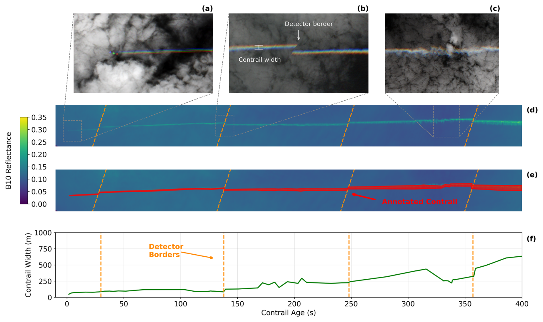
Figure 3 (a) Sentinel-2 true colour image showing the aircraft and the contrail in the first 10 s. (b) Sentinel-2 true colour image of the contrail after 140 s showing discontinuity caused by the detector border. (c) Sentinel-2 true colour image showing how the contrail loses its linearity after the wake vortex pair has broken down. (d) Sentinel-2 B10 top-of-atmosphere reflectance of the contrail. The vertical dimension of the image has been increased by a factor of 2 as compared to the horizontal dimension to improve the visibility of the contrail. (e) Same as panel (d), with manually annotated contrail polygon. (f) Contrail width as a function of contrail age. Dashed lines indicate the locations of the detector borders. Panels (a)–(e) contain modified Copernicus Sentinel data 2021.

An example of a Sentinel-2 annotation and the corresponding estimated contrail width is given in Fig. 3. As mentioned before, while the green visible band is used for the annotation, we visualise the cirrus band in Fig. 3d for clarity. The estimated contrail width (see Fig. 3f) is not found to be a smooth function of contrail age: several “jumps” are noticeable for contrail ages larger than 100 s. These jumps are in part due to the contrail crossing detector boundaries: which introduces discontinuities in the contrail annotation (see Fig. 3b). However, the remainder of the variability in Fig. 3 corresponds to the breakdown of the wake vortex pair. In other annotations such as Fig. D3, we can directly see the inception of the Crow instability (Crow, 1970) which ultimately leads to the breakdown of the vortex pair.

2.8 Evaluation of the Schmidt–Appleman criterion and comparison to literature

We assess the agreement between SAC predictions and satellite observations using a contingency table, given in Table 3, which classifies each prediction as a true positive (TP), false positive (FP), false negative (FN), or true negative (TN).

Table 3 Contingency table for the validation of the SAC against satellite observations.

The entries of the contingency table are combined into metrics that are used to assess the performance of the SAC. Specifically, we make use of the precision Pr and recall Re which are defined by

$$\begin{array}{}\text{(7)}& \mathrm{Pr}={\displaystyle \frac{\mathrm{TP}}{\mathrm{TP}+\mathrm{FP}}},\mathrm{Re}={\displaystyle \frac{\mathrm{TP}}{\mathrm{TP}+\mathrm{FN}}}.\end{array}$$

The precision corresponds to the fraction of predicted contrails that are observed, and the recall corresponds to the fraction of observed contrails that were also predicted to form. They have been used previously to quantify the performance of contrail forecasts by Geraedts et al. (2024) and Meijer (2024).

In addition to using the dataset created in this work, we also use two existing observational datasets of contrails for quantifying the performance of the SAC. These are the dataset presented by Low et al. (2025) and the dataset described by Jarry et al. (2026), both of which consist of contrails found in ground-based camera images. We also compare the differences in SAC performance found when switching meteorological data sources to the results by Gierens et al. (2020).

Both Gierens et al. (2020) and Low et al. (2025) directly provide entries of the contingency table, which we use to compute precision and recall according to the definitions above. In contrast, Jarry et al. (2026) do not provide these numbers and we therefore process their dataset to obtain the entries of the contingency table. Their dataset consists of ground-based camera images with contrail annotations that are matched to flights passing through the camera field of view (FOV) based on ADS-B data, not limited to IAGOS aircraft. In order to be included in the contingency table, we require that (1) the camera zenith angle is limited to a maximum of 60° to avoid geometric distortion near the image borders; (2) only flights above an altitude of 7 km are considered, as lower-altitude aircraft are not expected to form contrails; 3) flights without a valid flight_id are discarded to avoid erroneous matches caused by unreliable ADS-B data. For each remaining flight we determine whether it formed a contrail by checking for annotations with the relevant flight_id in the images where the flight is within the FOV and images after the flight exited the FOV. The SAC has been computed for each flight with an overall propulsion efficiency of 0.30 (0.35 and 0.40 were also tested but resulted in lower precision values) using temperature, humidity and pressure from the ECMWF ERA5 reanalysis dataset (Hersbach et al., 2020).

3 Results and discussions

3.1 Contrail dataset overview

The application of the collocation process to IAGOS data for the years 2013 to 2022 has resulted in a total of 543 annotated collocations (366 in Sentinel-2 imagery and 177 in Landsat 8/9 imagery). For 195 of these Sentinel-2 collocations, we have annotated the contrail that is being formed by the IAGOS aircraft. The spatial and temporal distribution of the collocations are shown in Fig. 4. Most collocations are found over (or close to) land masses, since the Sentinel-2 and Landsat satellites are primarily used for land observations. IAGOS aircraft have been collocated in climb (54 times), cruise (455 times) and descent (34 times) phases. The mean geometric (GNSS) altitude of the collocations is 10.5 km, with 90 % of the collocations being above 9.0 km. Further details on the vertical distribution of the collocations are discussed in Sect. 3.2. Figure 4b shows that almost all collocations occur from 2017 onward, with a single exception in 2013. The limited availability of data between 2013 and 2018 can be attributed to an error in the IAGOS data acquisition until 2018. The affected measurements have since been corrected, but all repaired data carry a validity flag of 2 and are therefore excluded from the analysis. Additionally, the decrease in 2020–2021 can be attributed to a reduced number of flights during the COVID-19 pandemic. In the period 2017 to 2021, the Sentinel-2 program had two satellites operational, compared to only one Landsat satellite (Landsat 9 was only commissioned at the end of 2021), resulting in more Sentinel-2 collocations.

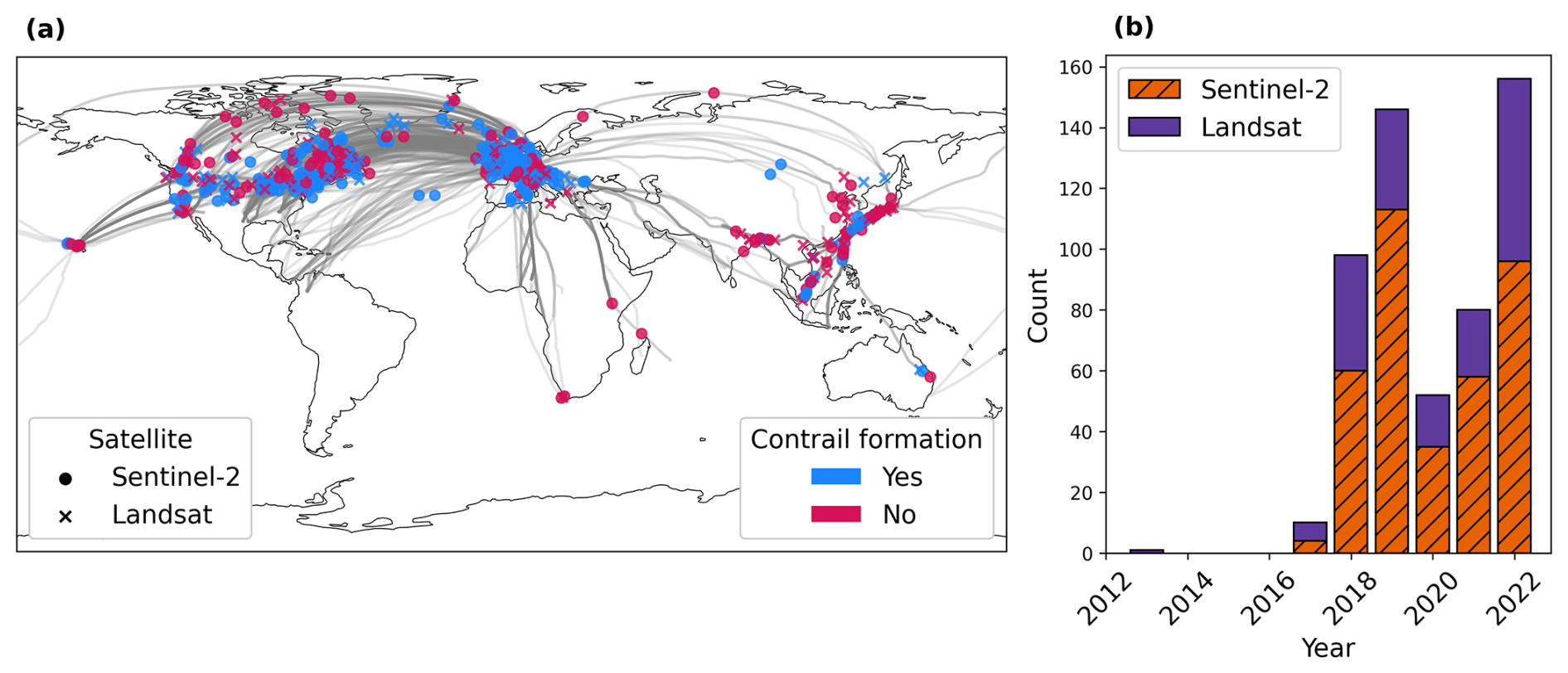
Figure 4 (a) Location of the 543 annotated collocations coloured by satellite. Grey lines indicate the flight paths of the collocations. (b) Histogram of scanning time of the collocations summed by year.

Table 4 Number of collocations for each aircraft within the IAGOS fleet, along with information on the aircraft and engine type. Aircraft without collocations and/or flights during the period of this study are included for completeness.

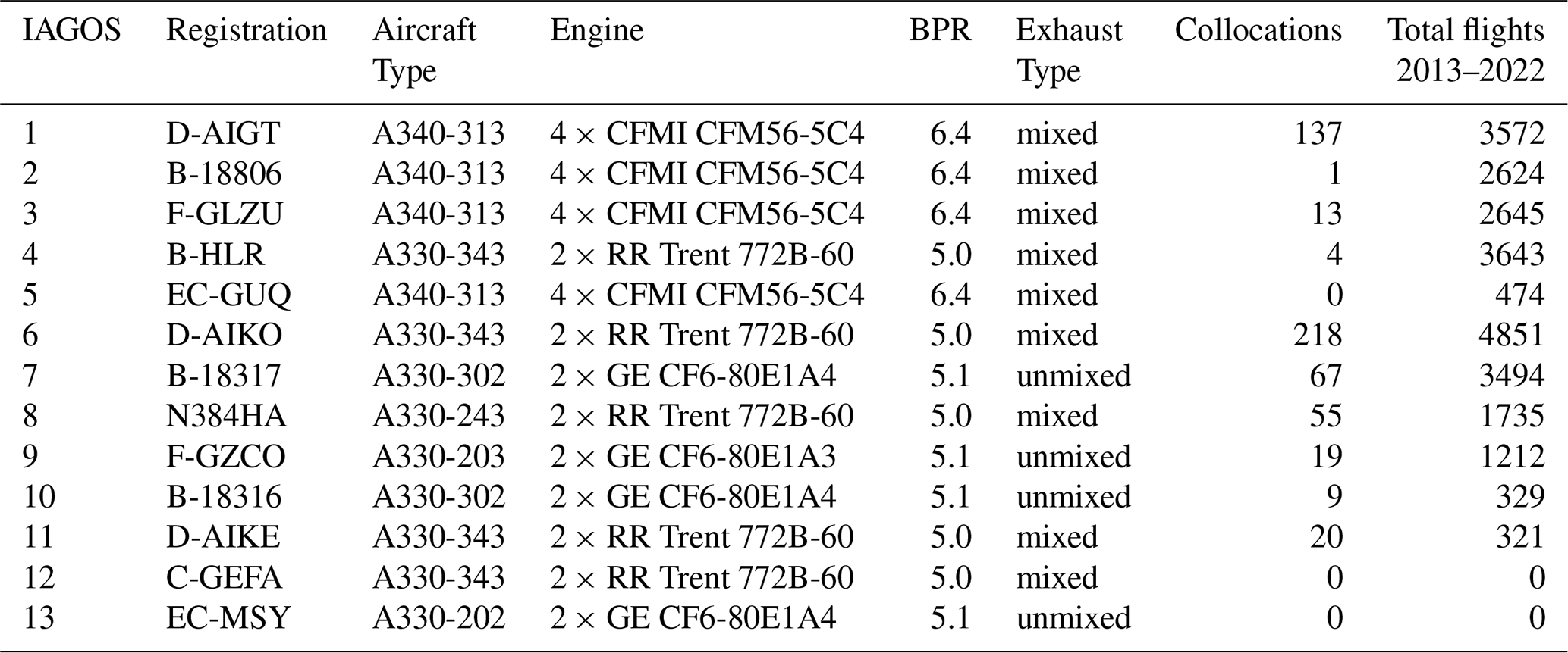
The number of collocations found for each aircraft in the IAGOS fleet as well as the total number of flights during the years 2013 to 2022 are given in Table 4, along with details on the aircraft type and engine. The IAGOS fleet covers bypass ratios between 5.0 and 6.4. These subsequent results may therefore not apply to modern lean-burn or high-bypass engines. Since both Sentinel-2 and Landsat satellites operate in sun-synchronous orbits, each location on Earth is observed consistently at the same local time. Consequently, the number of collocations associated with each aircraft is strongly influenced by typical flight routes and departure schedules. For example, F-GZCO recorded 474 flights in 2022, yet only 10 collocations were identified. During this period, the aircraft predominantly operated routes across Europe and North-Africa, with 86 % of departures occurring after the local satellite revisit time. In contrast, aircraft operating inter-continental routes, such as transatlantic flights, have a higher probability of being collocated, as their trajectories can be captured by multiple satellite overpasses.

3.2 Evaluation of contrail formation predictions by the Schmidt–Appleman criterion

For each collocation within the dataset, we evaluate the Schmidt–Appleman criterion (SAC) using both IAGOS and ERA5 data and compare this to the corresponding annotation. One such comparison is given in Fig. 5, for a case where no contrail formation is observed. The overall propulsion efficiency used within the evaluation of the SAC is derived from the PS model using IAGOS data as input: this is used to construct the threshold mixing line in Fig. 5. The shaded area represents the envelope of threshold mixing lines resulting from varying the efficiency by ±15 %. The ambient conditions obtained from ERA5 and IAGOS data are both shown in Fig. 5. In this particular case, the SAC evaluated using ERA5 data incorrectly predicts that contrail formation should occur. When using the IAGOS data however, the SAC is not satisfied in agreement with the observation. We give three more of these examples in Appendix A1, using both Sentinel-2 and Landsat imagery. The example provided in Fig. 5 shows a difference in ERA5 and IAGOS-based air temperatures of 1.9 K, which is on the higher end of the examples in the dataset. Over the whole dataset, we found a mean difference of −0.583 K (T_ERA5−T_IAGOS), with a standard deviation of 0.757 K.

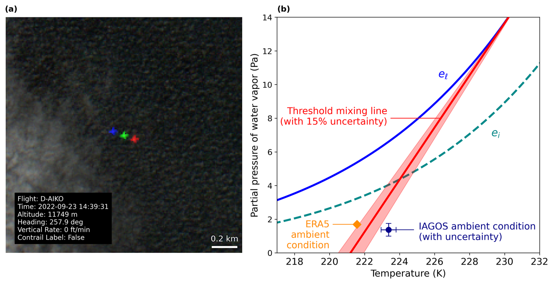
Figure 5 (a) Sentinel-2 true colour image showing the D-AIKO aircraft without a contrail. The rainbow effect (i.e. three differently coloured aircraft being visible) arises from the staggered configuration of the sensing instrument, which introduces a small time offset between the individual bands. This time delay results in a parallax difference between the bands. (b) Corresponding SAC diagram including saturation pressure w.r.t. liquid (e_l) and ice (e_i); the threshold mixing line resulting from the PS model overall propulsion efficiency; the ambient conditions from ERA5; and the IAGOS measurements with uncertainties. Contains modified Copernicus Sentinel data 2022.

Table 5 Summary of performance metrics for the SAC compared against the satellite observations of contrail formation for IAGOS and ERA5 weather data. Bold row indicates best performing dataset.

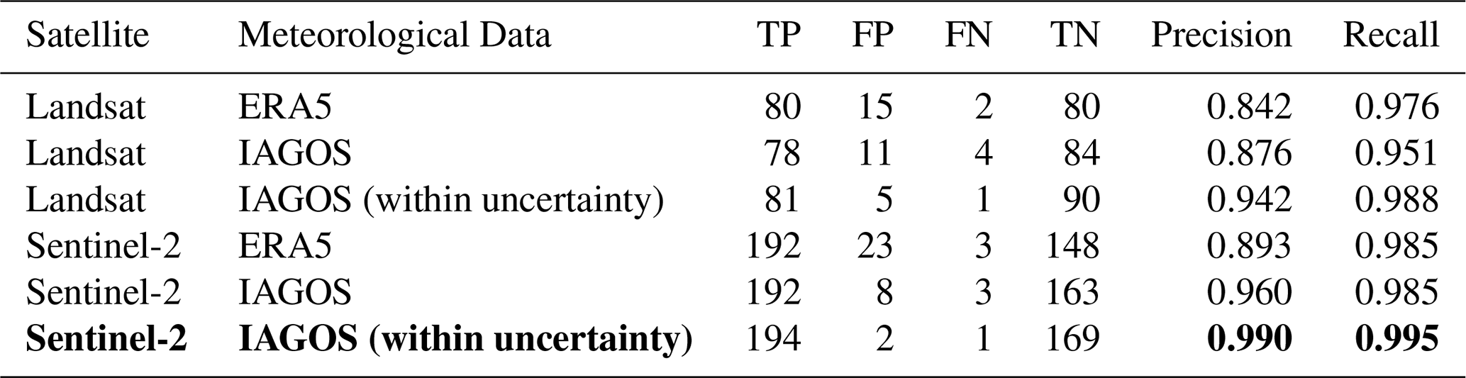
The results from the evaluation of the SAC predictions using the entire dataset are given in Table 5 as a function of the satellite platform and meteorological data used. For the “IAGOS (within uncertainty)” meteorological data source, we consider the SAC prediction to be correct if any combination of temperature and relative humidity values within the 95 % confidence intervals leads to a correct prediction (see the examples in Figs. A1 and A2). We now discuss the results in Table 5 by focusing on the effect of observation quality, the effect of the meteorological data source and by comparing the results to the literature. Firstly, for identical weather data, observations based on Landsat exhibit a consistently lower precision than those based on Sentinel-2, with differences ranging from 0.048 to 0.084, while recall remains comparable between the two (differences < 0.034). The lower SAC precision for Landsat observations is driven by a relative increase in false positives, where the SAC is satisfied but no contrail is observed. This reduction in precision when using Landsat instead of Sentinel-2 observations is found to be statistically significant (p-value of 5 %), and we hypothesise that the reduced resolution of the Landsat RGB imagery compared to the Sentinel-2 RGB imagery (30 m instead of 10 m) leads to a larger number of contrails that are unobservable. During the early part of the jet phase (below 10 s), the widths of the vortices are in the order of 10's of meters. As a consequence, an instrument with a coarser spatial resolution of 30 m might struggle to detect these features since more background radiation is coming into a pixel, reducing the contrast with the background. Examples of how a reduced image resolution complicates the contrail observation process can be found in Appendices A and D. To assess the possibility that the observed differences in precision and recall between the Landsat and the Sentinel-2 observations are due to sampling effects, we have performed Monte Carlo simulations (further explained in Appendix A2). The results indicate that under the null hypothesis that the precision and recall have the same value for the two satellites, the probabilities of finding the observed differences in precision and recall are 0.005 and 0.06 respectively. In other words, the observed differences in precision and recall for the two different satellites are unlikely to be explainable by random sampling effects alone.

Secondly, we see that the use of IAGOS instead of ERA5 data leads to better agreement between the SAC predictions and observations for both satellite instruments. The precision increases by 0.067 for the Sentinel-2 observations and by 0.034 for those from Landsat. In the analysis of Gierens et al. (2020), the SAC was calculated using ERA5 and compared against SAC calculated using IAGOS, which was considered the ground truth. Their results indicate a precision of 0.923 and a recall of 0.992. When we consider the SAC computed using IAGOS data as the ground truth – rather than the satellite observations – we find a precision of 0.932 which is within 1 % of the value found by Gierens et al. (2020).

Table 5 shows that the use of ERA5 data results in a larger number of false positives than when using IAGOS data as input for the SAC. One possible explanation for this is the reported mean cold bias of approximately 0.5 K in ERA5 temperatures (Wolf et al., 2025), which lowers ΔT_LC and can increase the number of false positive predictions by the SAC. The increase in false positives leads to a decrease in precision, without affecting recall.

In addition, we evaluated the effect of using the relative humidity of the clear-sky portion of the ERA5 grid point, calculated from specific humidity and cloud cover fraction (Tompkins et al., 2007). In 76 % of the collocations in Table 5 the cloud cover fraction was 0.0. In the remaining 24 % cases with partial cloud cover, the clear-sky RH_i did not have an effect on the predictions of the SAC.

Lastly, we discuss the evaluation results where the SAC prediction is considered to be correct if any combination of overall propulsion efficiency, air temperature or relative humidity values within the 95 % confidence intervals of IAGOS data leads to a correct prediction. This increases the precision to 0.990 (0.942) and the recall to 0.995 (0.988) for the Sentinel-2 (Landsat) observations. Thus, the SAC correctly predicts 99.2 % of Sentinel-2 observations and 96.6 % of Landsat observations when IAGOS measurement uncertainty is taken into account.

In other observational datasets, the level of agreement between observations and SAC predictions is found to be lower than that obtained using the dataset introduced here. Using the data from Low et al. (2025), we obtain a precision of 0.717 and an average recall of 0.982 across all waypoints. Similarly, using the dataset from Jarry et al. (2026), we obtain a precision of 0.444 and a recall of 0.973 when comparing annotated contrails with corresponding flight trajectories. In both ground-based studies, the reported precision is lower than that observed in the Landsat and Sentinel-2 results presented here. One contributing factor may be the spatial resolution of ground-based methodologies. At an altitude of 10 km, the all-sky camera used in Jarry et al. (2026), has an effective pixel resolution of approximately 50–100 m, which likely contributes to an increased number of false positives. However, the wide-angle camera used in Low et al. (2025), has a resolution at 10 km of approximately 5–10 m, higher than both satellites. We thus further attribute the remaining discrepancy to reduced observation quality inherent to ground-based camera methods, including the presence of low-level clouds, or sun glare effects. Overall, the higher precision reported by Low et al. (2025) compared to Jarry et al. (2026) is consistent with the hypothesis that spatial resolution is the dominant factor in contrail formation detection, which would also explain the higher precision found for Sentinel-2 observations relative to Landsat.

Effects of uncertainty in ambient conditions and overall propulsion efficiency

In Fig. 6a we show the collocations as a function of ΔT_LC and altitude, coloured according to the outcome of comparing the SAC prediction with the corresponding observation. Figure 6b focuses on incorrect predictions within the cruise altitude region, and shows the 95 % confidence interval of T_LC by using the IAGOS uncertainty for T and RH_l and the 15 % efficiency uncertainty leading to the upper and lower bounds of ΔT_LC. We see that even when accounting for uncertainty, 2 (5) false positives and 1 (1) false negatives for the Sentinel-2 (Landsat) are still present (as also presented in Table 5). Interestingly, several false positives identified using Landsat occur at ΔT_LC values between −3 and −4 K, which are more negative than the false positives found using Sentinel-2. This could be explained by the lower spatial resolution of the Landsat imagery relative to Sentinel-2, complicating the observation of contrail formation.

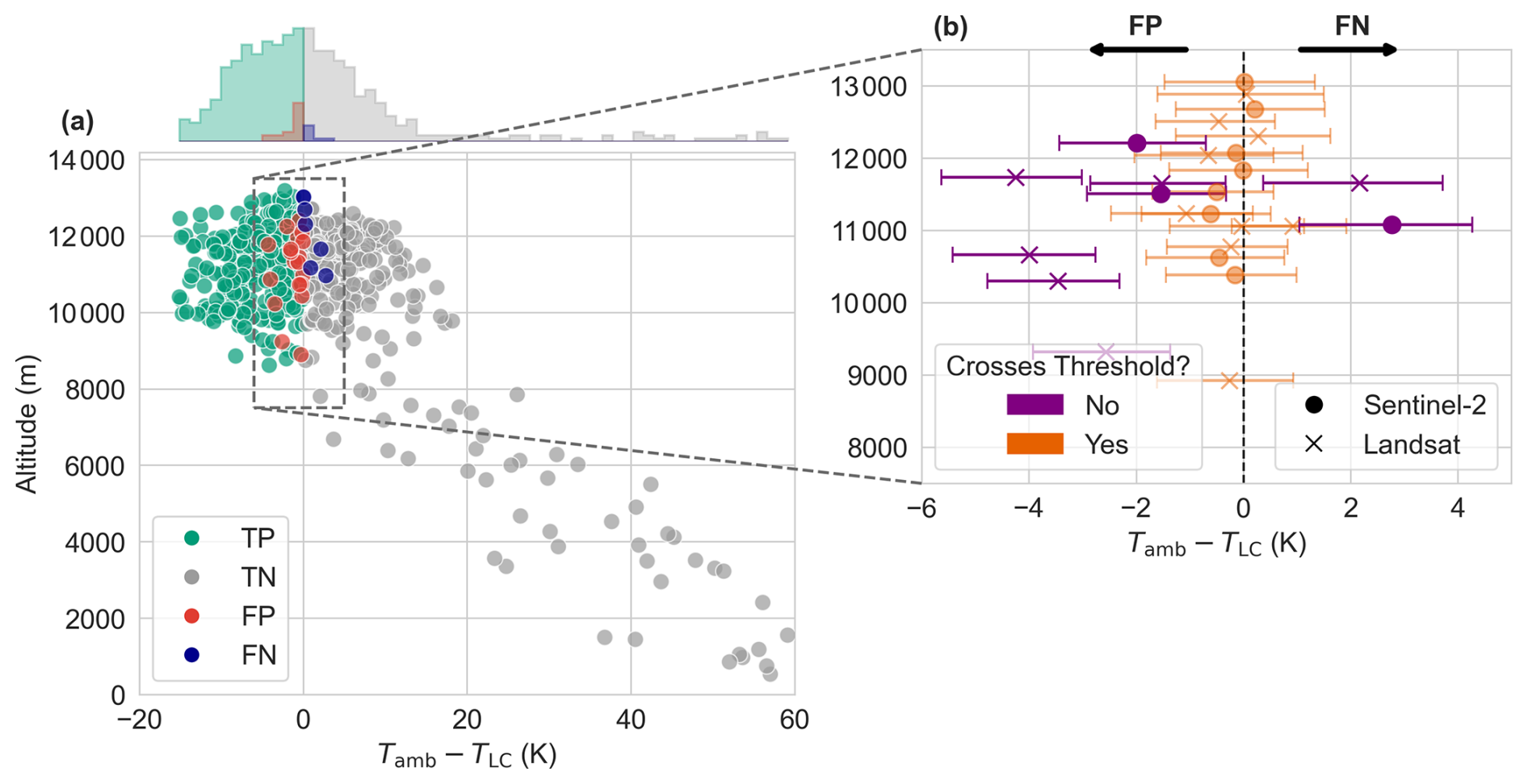
Figure 6 (a) All 543 collocations shown as a function of the temperature difference ΔT_LC (derived from the IAGOS measurements) and altitude, coloured according to the outcome of comparing the SAC prediction with the corresponding observation. The histogram above the plot displays the marginal distribution of ΔT_LC for each evaluation outcome. (b) Same as panel (a) but focusing on incorrect predictions in the cruise altitude region. Horizontal error bars represent 95 % uncertainty from overall propulsion efficiency and IAGOS measurements. The altitude of each point is randomly changed slightly to avoid overlap and for better clarity. Points crossing the contrail formation threshold are shown in orange whereas those that do not cross the threshold, even when accounting for uncertainty are shown in purple with lower opacity. Cross (circle) markers indicate that the contrail is observed in Landsat (Sentinel-2).

Figure 6b indicates that the uncertainty in the ΔT_LC is driven primarily by the overall propulsion efficiency uncertainty: which accounts for a change in ΔT_LC of ±0.66 K on average for all false positives and false negatives. The second largest driver of uncertainty for these false positives and false negatives is the air temperature, with an average change in ΔT_LC of ±0.41 K followed by RH_l with ±0.25 K.

Figure 6b shows that incorrect predictions are all located between GPS altitudes of 9 and 13 km, three of which are during the climb phase (not indicated in the figure) and the remainder during cruise. The spatial distribution of these erroneous predictions is consistent with the overall spatial distribution of the dataset (not shown). The false positives (false negatives) are all found between 217.0 K (220.5 K) and 224.6 K (228.7 K), with an average temperature of 220.5 K (223.4 K).

3.3 Contrail evolution

3.3.1 Lifetimes of observed contrails

The estimated lifetimes (corresponding to the estimated age of the end of the centerline of the polygon annotation) for the 195 contrails observed in Sentinel-2 imagery are shown in Fig. 7. We find that 48.2 % of contrail lifetimes are longer than 10 s (approximately the duration of the jet phase) and 8.7 % are longer than 120 s (approximately the end of the vortex phase). Contrails for which the annotation polygon ends at the satellite image swath edge, implying that the estimated lifetime is a lower bound on its actual lifetime, are shown using red markers in Fig. 7.

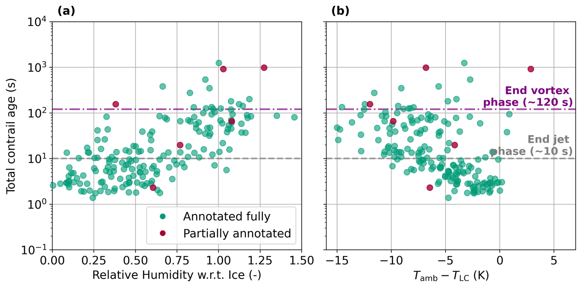
Figure 7 (a) Total contrail age in seconds against RH_i from IAGOS at the “oldest” point of the contrail. Contrails that leave the satellite image are coloured “red”, contrails that are fully annotated in the image are “green”. (b) Total contrail age in seconds against ΔT_LC from IAGOS at the “oldest” point of the contrail.

Figure 7a shows contrail age as a function of the IAGOS RH_i value at the oldest point of the contrail, indicating that mean lifetimes increase with increasing RH_i. A linear regression between RH_i and the logarithm of contrail lifetime yields R²=0.49. A similar analysis using ERA5 RH_i produces R²=0.51, suggesting a comparable relationship between humidity and contrail persistence in both datasets.

Contrails with lifetimes shorter than 10 s have a mean RH_i of 0.40±0.22 (1σ) (0.40±0.24) for IAGOS (ERA5) data. Those lasting between 10–120 s exhibit a mean RH_i of 0.76±0.32 (0.74±0.27), and contrails persisting longer than 120 s have a mean RH_i of 0.96±0.20 (0.99±0.14).

Contrails have been shown to persist in slightly ice-subsaturated air (Li et al., 2023; Petzold et al., 2025), which is consistent with our findings that contrails surviving past the vortex phase have a mean RH_i of 0.96±0.20. Four contrails have been found at RH_i below 90 %, which could also be attributable to the fact that the IAGOS temperature and relative humidity measurements are taken only at the moment the aircraft passes a location, whereas the observed contrail will have aged and been advected by the wind, leading to a spatial and temporal mismatch between the IAGOS measurements and the actual atmospheric conditions of the older points of the observed contrail. Another reason might be the response time of the IAGOS humidity sensor discussed in Sect. 2.2. Because the humidity sensor responds more slowly in colder temperatures, sharp humidity gradients are dampened and the measured RH_i may not represent the actual RH_i.

Figure 7b shows contrail age against the ΔT_LC, where more negative values indicate a higher maximum supersaturation w.r.t. liquid achieved during the mixing process of the engine exhaust and the ambient air. We see from Fig. 7b that generally, more negative values of ΔT_LC indicate longer-lived contrails, however the trend is weaker than that of RH_i. This is also visible in a lower R² value of 0.23 between the ΔT_LC and the logarithm of the contrail age. In four cases, a contrail was observed while having a ΔT_LC above 0, similar to the three Sentinel-2 observed contrails not predicted by the SAC (see Table 5).

3.3.2 Contrail width in the jet and vortex phases

We compute the contrail age and width using the methods described in Sect. 2.7 and interpolate the contrail width to 1 s intervals such that we can determine the mean width and 95 % confidence interval for every timestep. The resulting time series is shown in Fig. 8. An overview of the evolution of the width individual contrails can be found in Appendix B. Do note that the observed widths are subject to bias from the manual annotation process.

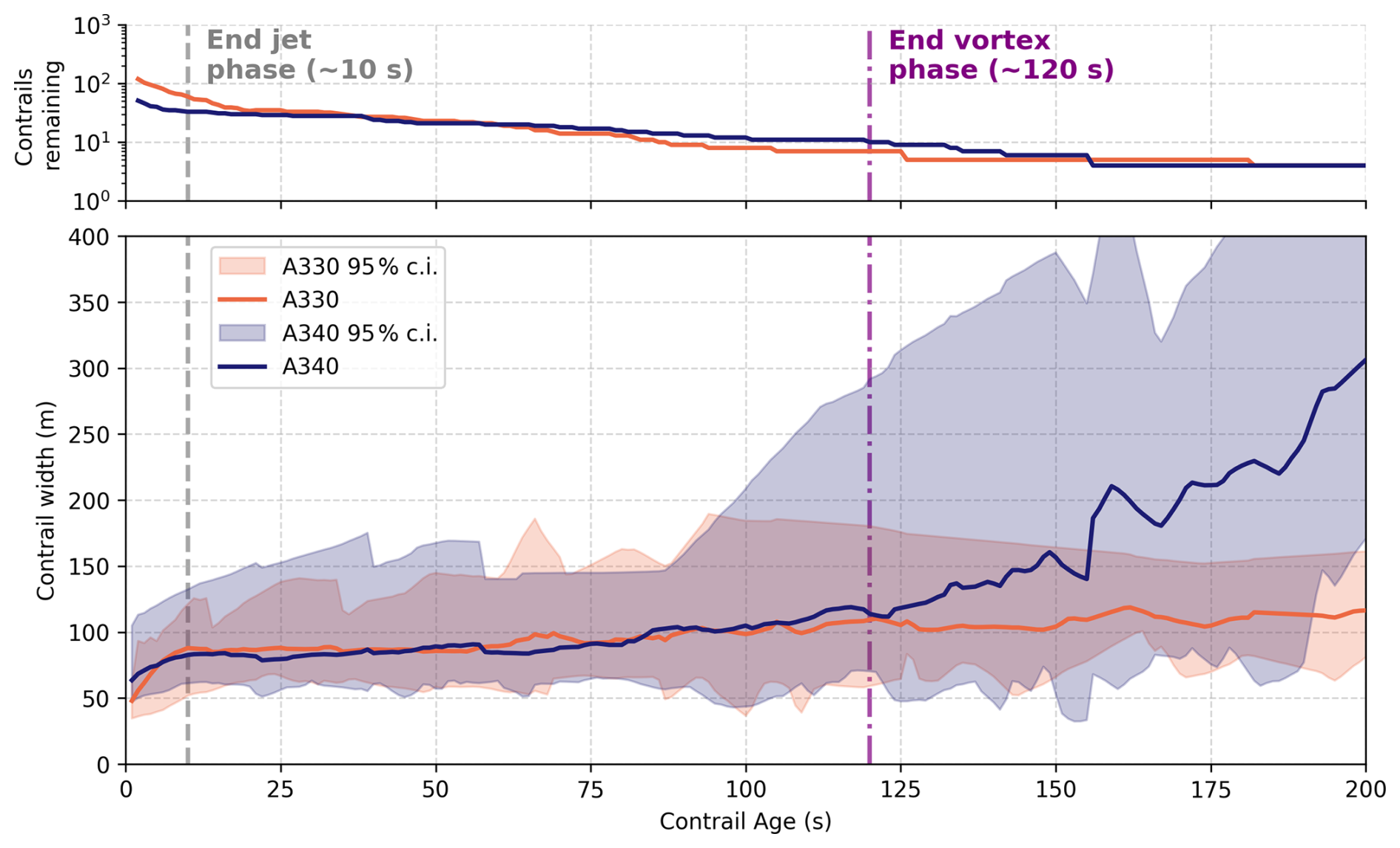
Figure 8 Statistics on the evolution of contrail width as a function of age. The number of surviving contrails as a function of age is given at the top. The approximate end of the jet phase (10 s) and end of the vortex phase (120 s) are indicated using dashed lines.

Figure 8 shows a jet and vortex width evolution pattern that is qualitatively consistent with previous observations (Hoshizaki et al., 1972) and with model simulations of the jet and vortex phases (Paoli and Shariff, 2016). The jet phase is characterised by continuous growth of the exhaust jets by turbulent mixing, followed by entrainment of the jets in the wake vortex pair after which mixing is inhibited and horizontal growth stagnates. For both aircraft types, the initial width in the jet phase is approximately 50 m, comparable to the initial wake vortex separation b₀ of 47.3 m for both aircraft types. At this point in the contrail lifetime, the two vortices are still visible in the satellite image as is shown in Fig. 3a. Subsequently, the contrail enters the vortex phase, during which the width remains constant at values between 80 and 100 m. Although the lateral extent of the contrail does not change substantially, the initially separated vortex pair gradually merges into a single uniform trail (as viewed from the satellite perspective) which is shown in Fig. 3b. Only 17 contrails survive for longer than 120 seconds, leading to an increasing spread in the observed width values beyond this point. Although the width of the A330 contrails is found to remain relatively constant after 120 seconds, the A340 contrails appear to resume growing beyond this point. However, the latter behaviour of the A340 contrails is dominated by a single contrail with significant horizontal growth: indicating the limited statistical significance of the width data beyond the vortex phase.

The value for the contrail width B₁ at the end of the vortex phase predicted by CoCiP using Eq. (6) is found to be approximately 20 m for both the A330 and A340 aircraft, assuming maximum take-off weight and V_a=250 m s⁻¹. This initial width is in a similar range to the widths presented in Fig. 4 from Schumann (2012), where the initial widths are reported to be between 10 and 30 m. Comparing this to Fig. 8, we conclude that the observed width is therefore a factor of 2–4 higher than that calculated in CoCiP. It should be noted however that the initial width has a relatively small impact on the evolution of the contrail within the dispersion phase modelled by CoCiP: the initial depth is considerably more important as it affects the rate of horizontal growth by vertical wind shear. The CoCiP implementation in pycontrails (Shapiro et al., 2026) uses the wake vortex separation as a starting point for the subsequent diffusion phase, which is closer to the values found here.

Remote-sensing based observations of contrail width have been reported previously (Freudenthaler et al., 1995; Sassen, 1997; Immler et al., 2008; Mannstein et al., 2010; Iwabuchi et al., 2012; Schumann et al., 2013; Low et al., 2025; Jarry et al., 2026), but primarily focus on contrails observed after the vortex phase. Alternatively, computational fluid dynamics (CFD) simulations, most commonly large-eddy simulations (LES), can also be used to derive the contrail width at various times in the jet and vortex phases. In Paoli et al. (2013), the jet phase of a contrail was simulated using LES for both two-engine and four-engine aircraft scenarios. While optical depths or contrail width are not specifically derived, the width can be derived from the spatial distribution of the simulated particles from the 2D cross-sections through the vortex center at 10 and 20 s after formation. Based on this approach, the contrail width is approximately 70 m (90 m) for the two-engine (four-engine) case at 10 s, increasing to about 80 m (100 m) at 20 s. Similarly, Paugam et al. (2010) presents estimates for contrail width in the early dispersion phase. In particular, they find a contrail width between 100 and 150 m at 160 s after formation. Both these results are comparable to the observed widths shown in Fig. 8. Lewellen and Lewellen (2001) presents LES results for a B747 contrail during the first 300 s of its evolution. A top-down view reveals a nearly constant contrail width of roughly 100 m between 10 and 100 s, after which the contrail begins to expand horizontally, albeit with signs of wake vortex breakup.

3.3.3 Comparing the observed evolution of contrail width in the dispersion phase with CoCiP predictions

The small number of contrails that survive the vortex phase and enter the dispersion regime in our dataset does not allow for robust statistical conclusions on the horizontal growth rates of contrails. However, we illustrate here how the observed evolution of a contrail can be compared to a model such as CoCiP for the three observed contrails that have lifetimes longer than 600 s. Future work can extend our analysis of observed contrails to aircraft outside of the IAGOS fleet, in order to apply this type of analysis to a much larger dataset.

The horizontal growth of the three oldest contrails in our dataset is shown in Fig. 9 together with the simulations from CoCiP. Note that all three contrails have a mean IAGOS RH_i above 100 %. Despite the limited sample size, the simulated contrail widths exhibit good overall agreement with the observations, as the average dispersion rate in CoCiP differs from the observed values by at most 38 %. Nevertheless, the small number of available cases limits the statistical robustness of this comparison.

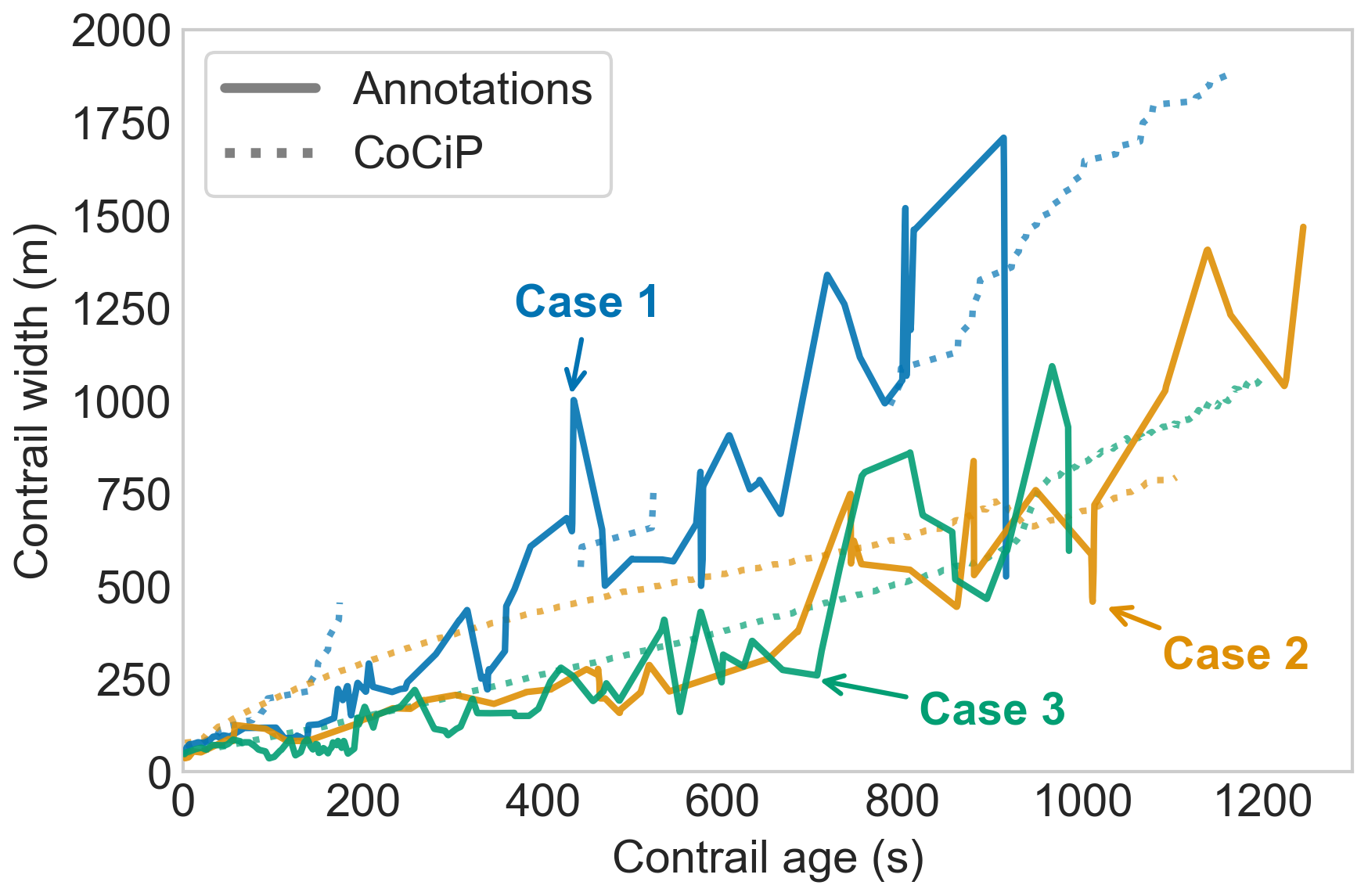
Figure 9 Evolution of contrail width (m) over contrail age (s) for the three cases that persist longer than 10 min. Different colours indicate the individual cases. Each CoCiP simulation used 1 s timesteps and a maximum contrail age of 20 min. Relative humidities (RH_l and RH_i) from ERA5 were scaled with IAGOS measurements. For Case 1, breaks in the simulated contrail indicate segments that have sublimated before the satellite scanning time.

Our contrail dispersion results are consistent with observations from the literature. For example, Freudenthaler et al. (1995) report ground-based LIDAR observations of contrails having width growth rates between 18 and 140 m min⁻¹, which aligns well with the three contrail cases shown in Fig. 9, which exhibit growth rates of approximately 102, 56, and 49 m min⁻¹.

Additional Sentinel-2 and Landsat observations covering a wider range of atmospheric conditions, aircraft and engine types as well as contrail lifetimes, would therefore be valuable to enable a more quantitative validation of dispersion rates in CoCiP and other contrail evolution models.

4 Conclusions

We have presented a method for locating flying aircraft in high-resolution low Earth orbit (LEO) satellite imagery from Sentinel-2 and Landsat. We applied this method to the IAGOS aircraft fleet in order to create a dataset of observations of contrail formation and early evolution combined with in situ measurements of temperature and humidity. The resulting dataset has been used for the evaluation of model predictions of contrail formation by the SAC, and horizontal growth by CoCiP.

The final dataset consists of 543 collocated IAGOS aircraft, in which 277 cases of contrail formation were observed. Out of these 277 contrails, of which 195 were annotated, 48.2 % were found to persist for longer than 10 s (approximately the jet phase) and 8.7 % longer than 120 s (approximately the vortex phase). The maximum contrail age identified in the dataset is 1250 s. Relative humidity with respect to ice was found to correlate strongly with contrail lifetime, exhibiting a R² value of 0.49 with the logarithm of contrail age. Contrails with lifetimes longer than 120 s showed a mean RH_i of 0.96±0.20, with four contrails found at RH_i below 90 % suggesting that contrails can survive the vortex phase in ice-subsaturated air.

A comparison of observed contrail formation with predictions indicates that the SAC can explain 98.3 % of the observations when using temperature and relative humidity measured by IAGOS, when accounting for measurement uncertainty. When using meteorological data from the ERA5 reanalysis as input, we find that only 92.1 % of observations agree with predictions by the SAC. This reduced agreement between observation and predictions illustrates the importance of accurate input data when comparing models and observations, in order to isolate model errors from those present in the inputs. Additionally, we find that for the same meteorological data source (e.g. IAGOS) the agreement between SAC predictions and Landsat observations is consistently lower than when comparing against Sentinel-2 data. Specifically, the precision of the SAC is found to be lower for Landsat observations, whereas recall remains approximately equal. This is caused by more frequent predictions of contrail formation by the SAC where Landsat imagery shows no identifiable contrail. We attribute this difference primarily to the coarser spatial resolution of Landsat RGB imagery (30 m) leading to a larger fraction of contrails that are not detectable compared to the Sentinel-2 imagery (10 m). All together, these results emphasise the important role played by limitations in meteorological input data and observations when evaluating contrail models. We therefore hypothesise that lower levels of agreement between SAC predictions and observations reported in previous studies may have been caused by inaccurate NWP data and/or observations.

Furthermore, the dataset presented here contains 195 annotated contrails which can be used to study the early evolution of contrails. We used these annotations to analyse the evolution in contrail width as a function of age, and compared these to previous observations as well as CoCiP model predictions. During the first 10 s (approximately jet phase) we observe rapid increases in contrail width as the turbulent engine exhaust jets mix with ambient air. This growth levels off near 10 s as the exhaust jets become entrained in the wake vortex pair, and contrail width is observed to remain approximately constant until about 120 s (approximately end of the vortex phase) after which horizontal growth is resumed, presumably driven by turbulence and vertical wind shear. These observed patterns are consistent with previous observational and modelling studies. The limited number of contrails found to persist for longer than 10 min does not allow for robust statistical conclusions on the rate of contrail growth in the dispersion phase. We presented the three oldest contrails in the dataset as individual case studies, illustrating how observations of this kind can be compared against contrail models. A larger dataset, covering a wider range of atmospheric conditions and contrail lifetimes, would be required to evaluate modelled dispersion rates quantitatively.

Although the results of this study suggest that the SAC can predict contrail formation with a high level of skill (that increases with the quality of the meteorological input data used), we note that the dataset used covers only a limited number of aircraft-engine combinations. Specifically, the dataset consists of only 10 different aircraft, which are all part of two wide-body aircraft families and are equipped with three different engine families. Future work can utilise the collocation methodology presented here, possibly augmented by automated contrail detection techniques, to increase both the size and coverage of the dataset. This will enable the evaluation of the SAC for a broader set of aircraft and engine combinations, as well as study the early evolution of contrails formed by different aircraft. Secondly, because the LEO observations used in this work resolve contrails well before they become detectable in geostationary imagery, they provide an intermediate ground truth for the position of a contrail and for its advection during this interval. Such constraints could support the attribution of geostationary-detected contrails to individual flights. Another avenue of future work is to infer additional information on contrail microphysical properties as well as wake vortex pair instabilities and decay from the satellite imagery, which we have not attempted here.

Appendix A: Additional results for the Schmidt–Appleman criterion analysis

A1 Additional collocations with the Schmidt–Appleman criterion

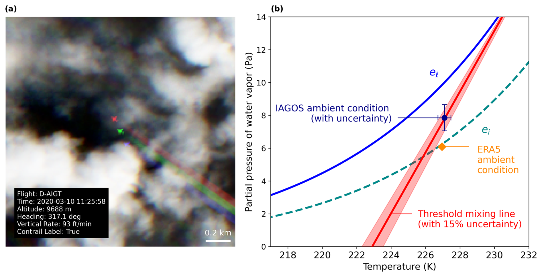
Figure A1 (a) Sentinel-2 true colour image showing the D-AIGT aircraft forming a contrail. The rainbow effect (i.e. three differently coloured aircraft being visible) arises from the staggered configuration of the sensing instrument, which introduces a small time offset between the individual bands. This time delay results in a parallax difference between the bands. (b) Corresponding SAC diagram including the threshold mixing line resulting from the PS model propulsion efficiency, the ambient conditions from ERA5, and the IAGOS measurements with uncertainties. Contains modified Copernicus Sentinel data 2020.

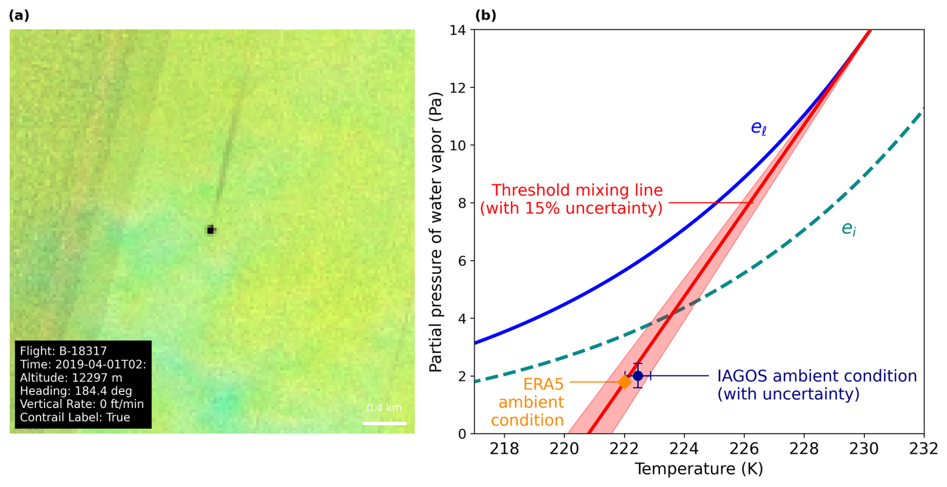
Figure A2 Same as Fig. A1, but for a Landsat false colour composite. Landsat-8 image courtesy of the U.S. Geological Survey.

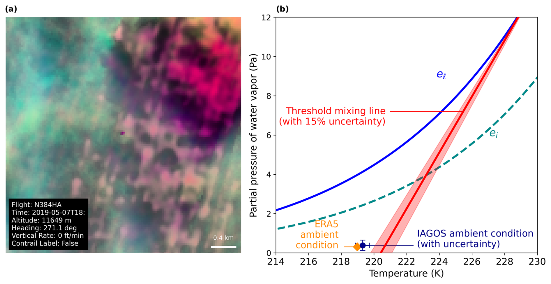
Figure A3 Same as Fig. A1, but for a Landsat false colour composite. Landsat-8 image courtesy of the U.S. Geological Survey.

A2 Statistical robustness of SAC precision and recall differences

We use a Monte Carlo simulation to assess the possibility that the observed differences in precision and recall between the Landsat and Sentinel-2 observations are a sampling artifact resulting from a small dataset size. We combine the contingency table entries obtained for the Landsat and Sentinel-2 observations (see Table 5) to compute the base rate s, recall Re and false alarm rate F. The expressions for the base and false alarm rate are

$$\begin{array}{}\text{(A1)}& s={\displaystyle \frac{\mathrm{TP}+\mathrm{FN}}{n_{\mathrm{landsat}}+n_{\mathrm{sentinel}}}},F={\displaystyle \frac{\mathrm{FP}}{\mathrm{FP}+\mathrm{TN}}}.\end{array}$$

These three parameters s, Re, F, calculated as 0.51, 0.97, and 0.07 respectively, define the parameters necessary for generating a distribution of precision and recall values under the null hypothesis that both datasets are random samples drawn from the same underlying process.

Using the baseline parameters $(s,\mathrm{Re},F)$, we generate m = 10 000 samples of size n, where n corresponds to the sample sizes of the Landsat and Sentinel-2 datasets. From each synthetic contingency matrix, we compute precision and recall as

$$\begin{array}{}\text{(A2)}& {\displaystyle }{\widehat{\mathrm{Pr}}}_i={\displaystyle \frac{{\mathrm{TP}}_i}{{\mathrm{TP}}_i+{\mathrm{FP}}_i}},\text{(A3)}& {\displaystyle }{\widehat{\mathrm{Re}}}_i={\displaystyle \frac{{\mathrm{TP}}_i}{{\mathrm{TP}}_i+{\mathrm{FN}}_i}}.\end{array}$$

This yields empirical distributions of $\widehat{\mathrm{Pr}}$ and $\widehat{\mathrm{Re}}$ for both the Landsat and Sentinel-2 sample sizes, representing the expected variability in precision and recall due to random sampling alone. For each realisation, we compute the differences in performance metrics between the two datasets with

$$\begin{array}{}\text{(A4)}& {\displaystyle }\mathrm{\Delta }{\widehat{\mathrm{Pr}}}_i={\widehat{\mathrm{Pr}}}_{\mathrm{sentinel}}^{\left(i\right)}-{\widehat{\mathrm{Pr}}}_{\mathrm{landsat}}^{\left(i\right)},\text{(A5)}& {\displaystyle }\mathrm{\Delta }{\widehat{\mathrm{Re}}}_i={\widehat{\mathrm{Re}}}_{\mathrm{sentinel}}^{\left(i\right)}-{\widehat{\mathrm{Re}}}_{\mathrm{landsat}}^{\left(i\right)}.\end{array}$$

These samples define empirical distributions of precision and recall differences under the null hypothesis of identical underlying performance. We denote the observed differences in precision and recall between the Sentinel-2 and Landsat as ΔPr_obs and ΔRe_obs, which we can read from Table 5 to be respectively: −0.084 and −0.034. The probability that the observed difference arises from sampling variability alone is estimated as

$$\begin{array}{}\text{(A6)}& {\displaystyle }{P}_{\mathrm{Pr}}=\mathbb{P}\left(\mathrm{\Delta }\widehat{\mathrm{Pr}}\le \mathrm{\Delta }{\mathrm{Pr}}_{\mathrm{obs}}\right),\text{(A7)}& {\displaystyle }{P}_{\mathrm{Re}}=\mathbb{P}\left(\mathrm{\Delta }\widehat{\mathrm{Re}}\le \mathrm{\Delta }{\mathrm{Re}}_{\mathrm{obs}}\right),\end{array}$$

where the probabilities are evaluated using the empirical cumulative distribution functions of the samples.

We find for the two datasets, evaluated with IAGOS, a probability P_Pr=0.005 or P_Re=0.060 that the observed differences are explainable by random sampling alone. In other words, this means that the observed difference in precision and recall are unlikely to be explainable by random sampling effects alone.

A3 Aircraft performance model comparison

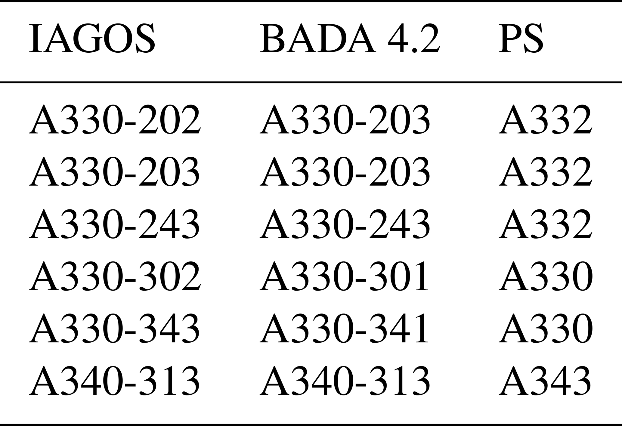
We used the BADA 4.2 and Poll–Schumann implementation in pycontrails. Not all aircraft types present in the IAGOS dataset (see Table 4) are explicitly represented in the BADA 4.2 files. For aircraft types without a direct match, a closely related aircraft type available in BADA 4.2 was used. For the Poll–Schumann model, aircraft were identified using their ICAO codes. The mapping between IAGOS aircraft types, the corresponding BADA 4.2 types, and the Poll–Schumann ICAO codes is shown in Table A1.

Table A1 Mapping between IAGOS aircraft types and corresponding BADA 4.2 and Poll–Schumann aircraft representations.

A3.1 Overall propulsion efficiency

In Fig. A4 we compare the overall propulsion efficiency, for both BADA 4.2 and PS, for all 543 IAGOS collocations. We can split the overall propulsion efficiencies into the three flight phases where climb corresponds to vertical rates greater than 0.508 m s⁻¹, cruise to absolute vertical rates below 0.508 m s⁻¹, and descent to vertical rates less than −0.508 m s⁻¹. The average values of the computed overall propulsion efficiencies for each phase and for each aircraft are shown in Table A2.

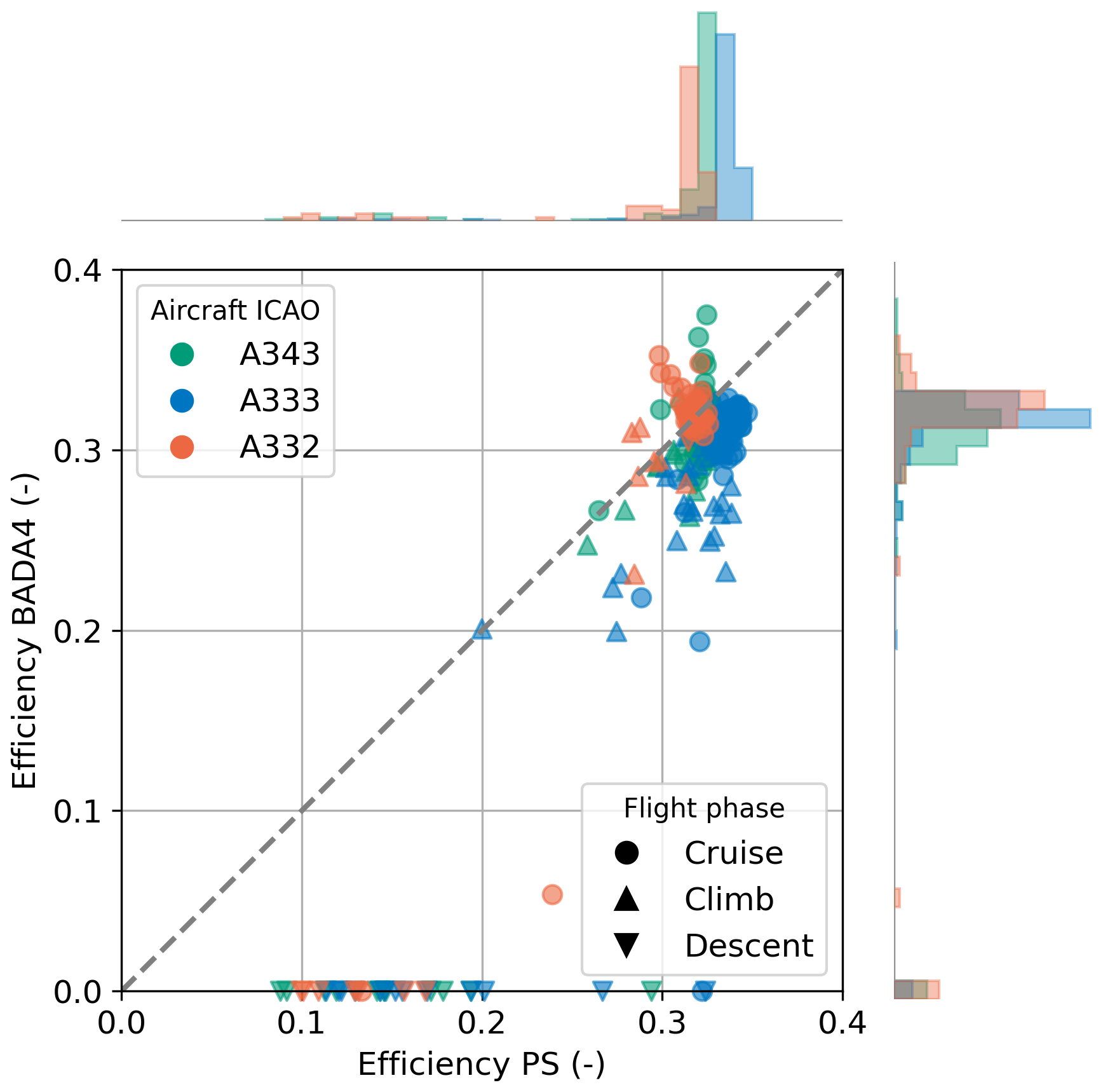
Figure A4 Scatter plot of overall propulsion efficiency in Poll–Schumann and BADA 4.2 at the scanning time of the satellite. Colour indicates IAGOS aircraft type, marker indicates flight phase. Histograms show the distribution of propulsion efficiencies shown with values scaled per aircraft type.

Table A2 Comparison of mean climb, cruise, and descent efficiencies from PS and BADA 4.2 APMs for collocations in IAGOS dataset using IAGOS weather data. Climb corresponds to vertical rates greater than 0.508 m s⁻¹, cruise to vertical rates with absolute values lower than 0.508 m s⁻¹, and descent to vertical rates less than −0.508 m s⁻¹.

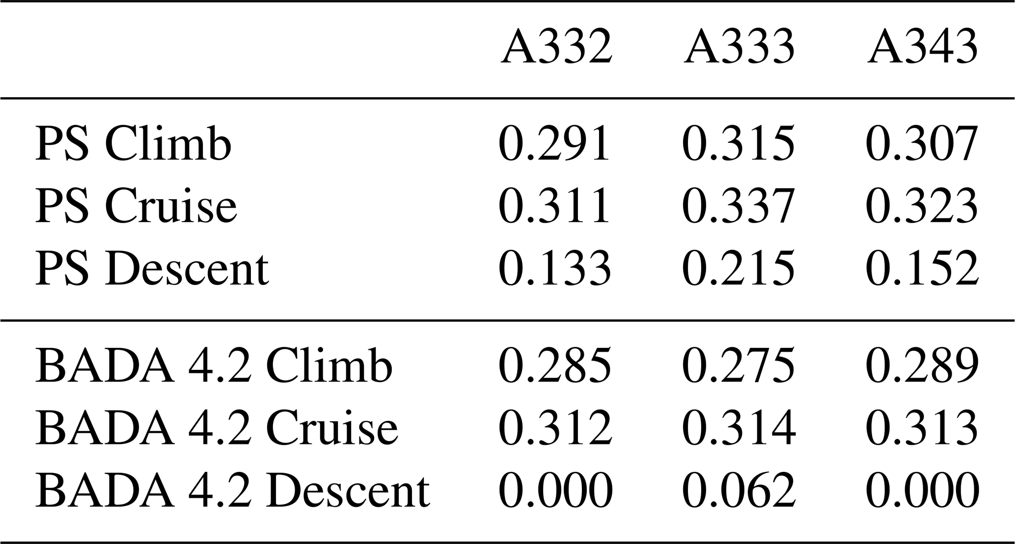
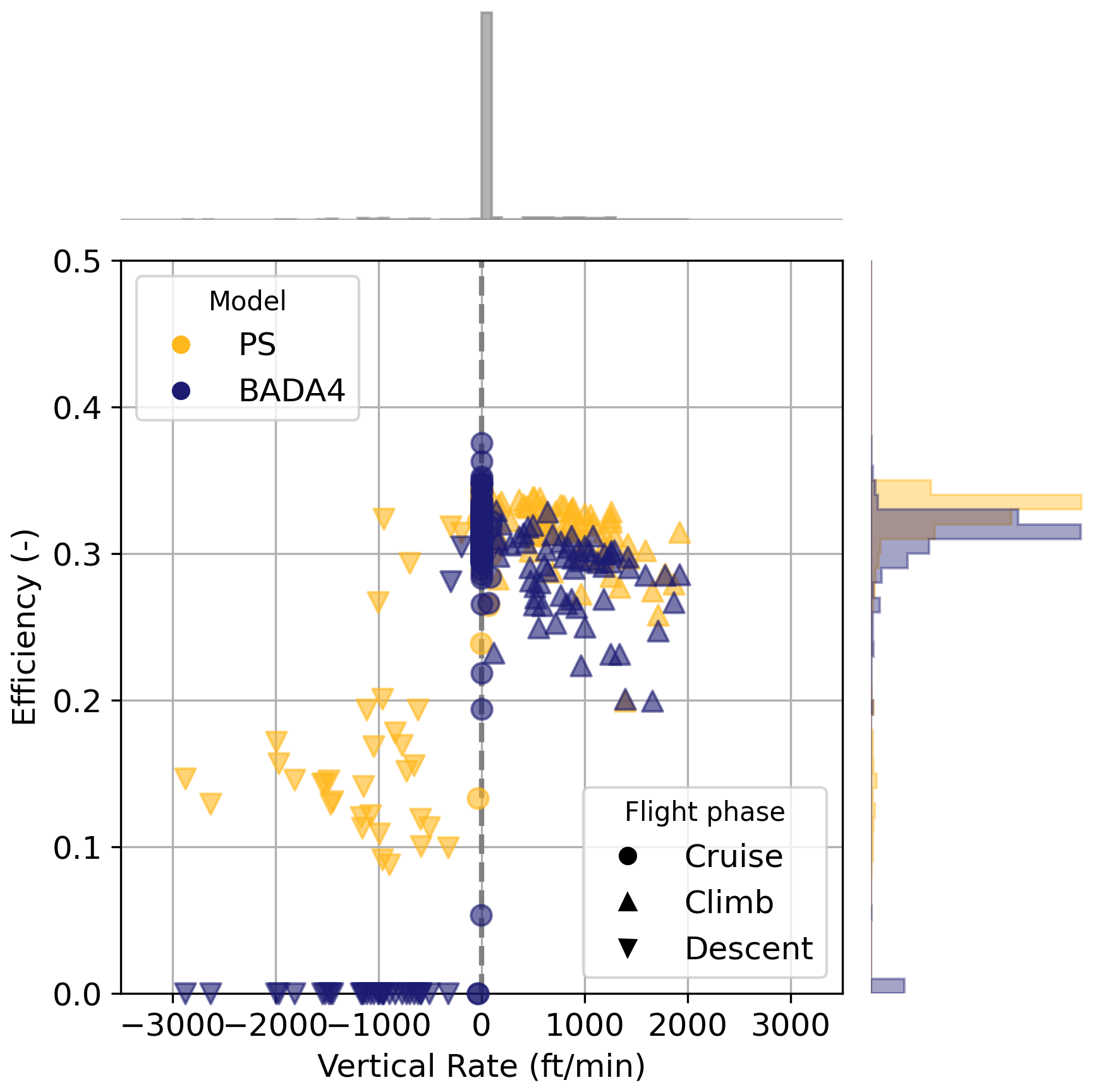
Figure A5 Scatter plot of overall propulsion efficiencies against the vertical rate at the scanning time of the satellite, coloured according to the model used. The histograms on the vertical axis show the distribution of efficiencies per model, and those on the horizontal axis show the distribution of vertical rates.

We see from this comparison that generally, during the climb and cruise phases, the efficiencies correlate well, with a root-mean-squared error of 0.0322, 0.0326, 0.0176, and a correlation coefficient r of 0.900, 0.609, and 0.515, for the A332, A333, and A343 respectively. For these two phases, the largest difference is found for the A333, where BADA 4.2 computes efficiencies that are on average approximately 0.03 lower than PS. However, during the descent phase, the difference between the two models is larger since the pycontrails implementation of BADA 4.2 computes an overall propulsion efficiency of 0 during descent. In contrast, PS computed efficiencies between 0.1 and 0.3 for these cases.

Figure A5 gives an alternative visualisation of this difference. Here, the overall propulsion efficiencies for BADA 4.2 and PS are shown against the vertical rate. At negative vertical rates, BADA 4.2 does consistently compute the overall propulsion efficiency as 0. Overall, as seen from the marginal distribution on the right, PS computes higher efficiencies than BADA 4.2, with PS computing efficiencies 0.01 to 0.02 higher than BADA 4.2.

A3.2 Influence on predictions using the Schmidt–Appleman criterion

We present the Schmidt–Appleman criterion (SAC) evaluation using BADA 4.2 efficiencies in Table A3. Compared to the PS results shown in Table 5, precision either increases slightly (by 0.01 to 0.02) or remains constant, while recall decreases in all cases by approximately 0.01 to 0.02. Both differences are consistent with BADA 4.2 underestimating efficiency relative to PS, which results in fewer contrail predictions by the SAC. This reduces the number of false positive predictions.

Table A3 Summary of performance metrics for the SAC compared against the satellite observations for IAGOS and ERA5 weather data. SAC computed with BADA 4.2 overall propulsion efficiencies. Bold row indicates best performing dataset.

Appendix B: Additional results for contrail width evolution

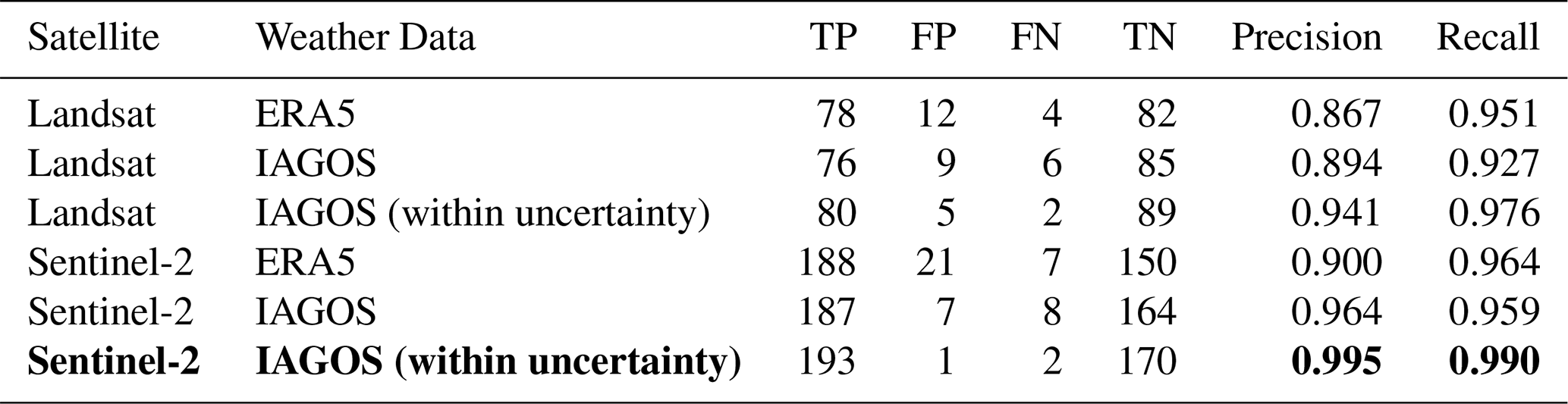
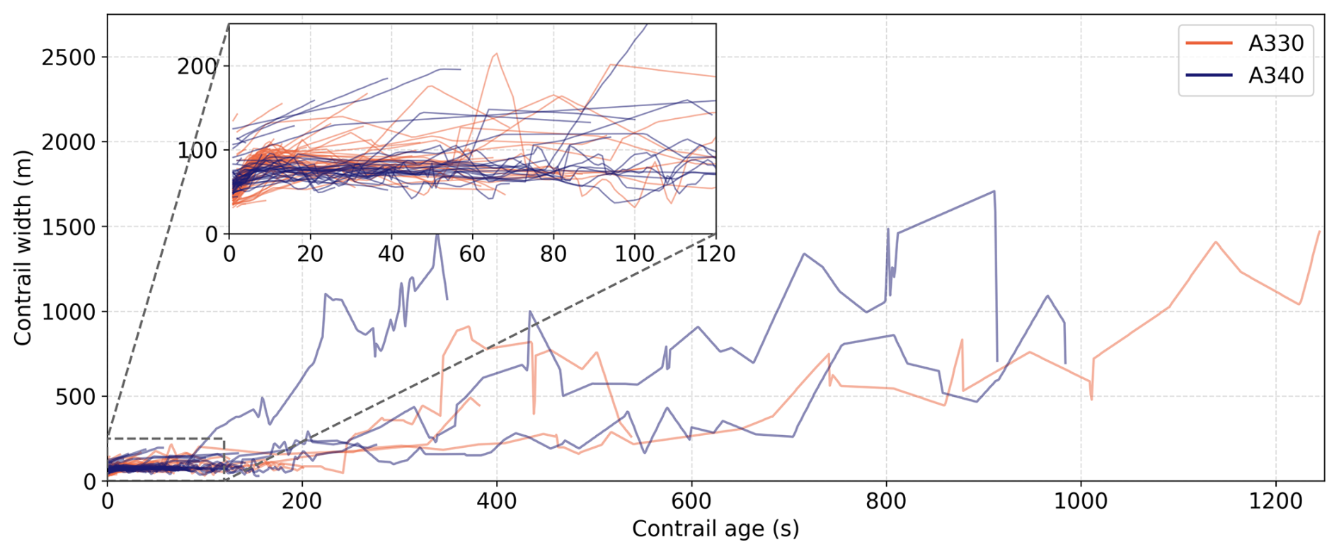
Figure B1 Evolution of contrail width as a function of age for all annotated contrails. The jet and vortex phase (first 120 s) are further visualised in the inset. Colours indicate aircraft family.

Appendix C: Additional details for the collocation process

C1 Satellite tile search

We used pycontrails (Shapiro et al., 2026) to identify Sentinel-2 and Landsat tiles containing IAGOS aircraft. This implementation uses a Google BigQuery table of Sentinel-2 satellite tiles, which provides the bounding box and nominal scanning time of the tile. For Landsat scenes, we query the USGS Landsat Collection 2 Bulk Metadata Service. For each available IAGOS flight trajectory, we then use these bounding boxes and the nominal scanning time to ascertain whether any trajectory waypoints might be found within an image. In cases where tiles overlap near the edges, only a single tile is kept to avoid duplication.

C2 Sentinel-2 metadata and processing steps

For the parallax and scanning time corrections (described in Appendix C4) we require viewing angle data at pixel-level (10 m) resolution as well as the satellite ephemeris and the detector time offsets.

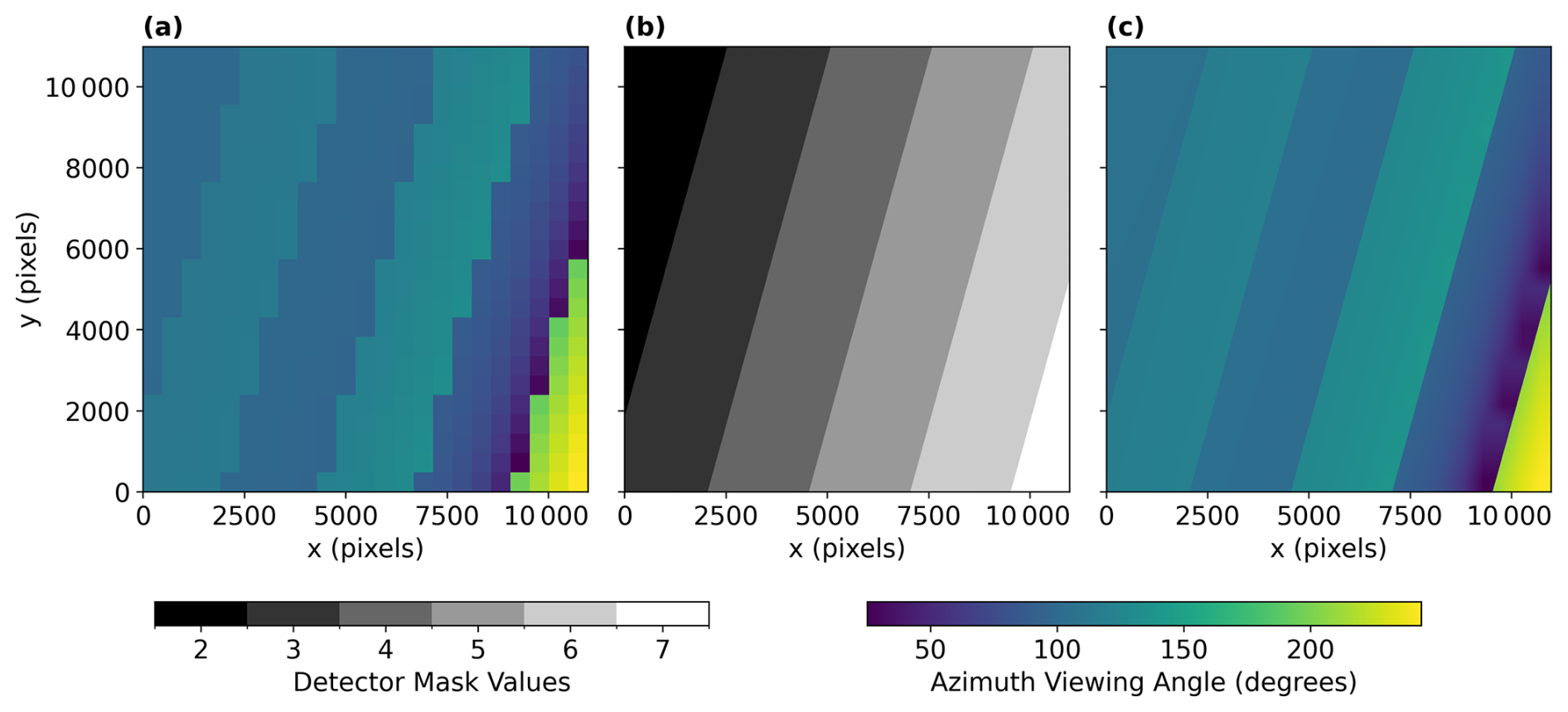
Figure C1 (a) Viewing azimuth angles for a single Sentinel-2 satellite image. (b) Detector pixel mask. (c) Viewing azimuth angles interpolated to pixel-level resolution.

We extract viewing angles (zenith and azimuth) from the tile metadata file (MTD_TL.xml, (Copernicus, 2024)) for every Sentinel-2 tile. These angles are provided at a coarse resolution of 25×25 km. The zenith angles are independent of the detector used to scan a pixel, meaning that we can interpolate them directly to the higher pixel-level resolution using bilinear interpolation. However, the azimuth angles exhibit staggered discontinuities at the detector borders (as shown in Fig. C1a) which need to be taken into account when interpolating this data. We utilise the pixel-level detector footprint mask provided in the Quality Indicator folder (QI_DATA; Copernicus, 2024) to ascertain which detector captured each pixel (see Fig. C1b). We then separate the coarse azimuth values by detector, bilinearly interpolate each detector's azimuth angles, and subsequently merge them using the detector mask. The resulting high-resolution azimuth viewing angles are shown in Fig. C1c.

The ephemeris data are available in the Satellite Ancillary Data in the Datastrip metadata file (MTD_DS.xml; Copernicus, 2024). The ephemeris contains the dated positions (x, y, and z) in Earth-Centered, Earth-Fixed (ECEF) coordinates in mm, along with the GPS time. The GPS time has been converted to UTC, using an 18 s offset (Seeber, 1993).

The detectors in the Sentinel-2 MSI alternate between pointing forward and backwards. For each satellite image, the Sensor Configuration metadata (Copernicus, 2024) provides the syncing times for each detector. The time delay per detector Δt_detector is found by computing the difference between the individual detector's syncing time and the average syncing time of all detectors.

C3 Landsat metadata and processing steps

After determining relevant Landsat scenes intersecting IAGOS aircraft, we use the USGS/EROS Machine-to-Machine API (U.S. Geological Survey, 2026) to download scene imagery, per-pixel viewing angle data, and other necessary metadata to compute aircraft collocations. Table C1 shows the exact request.

Table C1 Files retrieved via the USGS/EROS M2M API for each candidate Landsat scene.

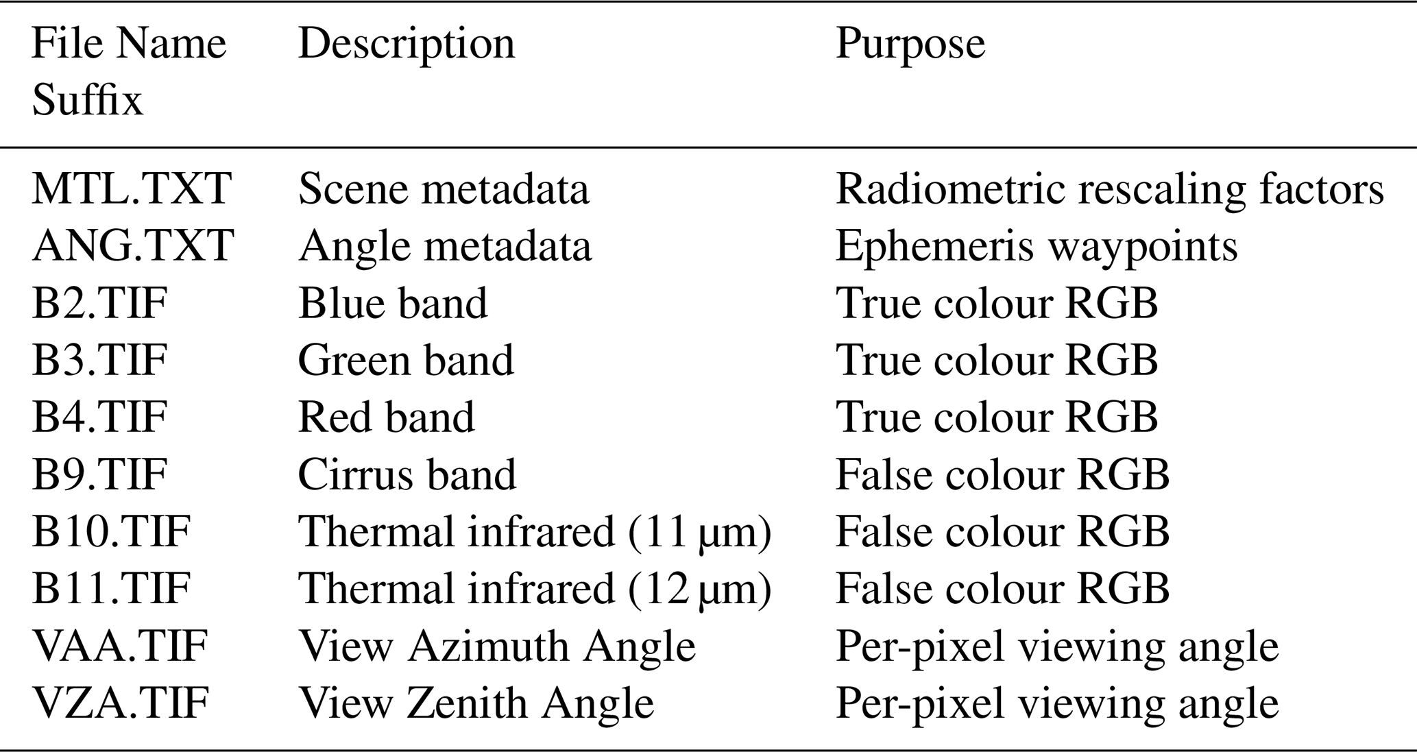
The per-pixel viewing zenith and azimuth angles (VZA and VAA) are provided at native spatial resolution and therefore do not require interpolation. The satellite ephemeris positions contained in the metadata are converted from ECEF coordinates to the scene's UTM coordinate reference system, and the satellite ground-track direction is estimated from consecutive waypoints. Unlike Sentinel-2, Landsat products do not explicitly provide the detector identifier for each pixel. To approximate detector membership, we leverage the view azimuth geometry: pixels are classified as forward- or aft-looking relative to the mean ground-track direction, thereby separating the focal plane into even and odd detector groups. A fixed temporal offset of ±2 s is then assigned according to this classification to approximate the scanning time offset Δt_detector (see Appendix C4).

C4 Collocation algorithm

We first transform the flight trajectory coordinates from IAGOS to the local UTM coordinate system used by the relevant Sentinel-2 or Landsat tile. Then, each waypoint (x_UTM, y_UTM, and z) at t_flight is corrected for parallax displacement using an iterative approach starting with (x_UTM, y_UTM). The position is updated according to

$$\begin{array}{}\text{(C1)}& {\displaystyle }{x}_{i+\mathrm{1}}=x_i-z\cdot \tan \left(\mathrm{VZA}(x_i,y_i)\right)\cdot \sin \left(\mathrm{VAA}(x_i,y_i)\right),\text{(C2)}& {\displaystyle }{y}_{i+\mathrm{1}}=y_i-z\cdot \tan \left(\mathrm{VZA}(x_i,y_i)\right)\cdot \cos \left(\mathrm{VAA}(x_i,y_i)\right),\end{array}$$

where VZA denotes the viewing zenith angle, VAA the viewing azimuth angle and i the iteration index. An iterative approach is necessary because as the position (x_i,y_i) changes, the zenith and azimuth angles change as well. This has an especially large effect near the detector boundaries since the azimuth angle changes discontinuously across the detector border (see Fig. C1c). In this study, five iterations were used. The result of this iterative process at time t_flight is denoted as (x_proj(t_flight), y_proj(t_flight)) in what follows.

To estimate the scanning time, we first transform the satellite ephemeris into the UTM coordinate system of the satellite image. This produces a satellite ground-track (x_sat(t_scan), y_sat(t_scan)). For each pixel with coordinates (x_proj, y_proj) a line perpendicular to the satellite ground track is drawn. The intersection point of this perpendicular line with the ground track is the location on the ground-track that is closest to this pixel. The corresponding scanning time t_scan is then obtained as the time at which the ground-track position matches this point.

The detector-dependent time offset is obtained by identifying the detector corresponding to the pixel location (x_proj, y_proj). The scanning time offset Δt_detector for Landsat (see Appendix C3) or Sentinel-2 (see Appendix C2) related to that detector is added to the previously estimated scanning times

$$\begin{array}{}\text{(C3)}& t_{\mathrm{scan}}\leftarrow t_{\mathrm{scan}}+\mathrm{\Delta }{t}_{\mathrm{detector}}.\end{array}$$

We now have both the flight trajectory projected onto the ground surface (x_proj(t_flight), y_proj(t_flight)), as well as the hypothetical times at which the projected trajectory would have been seen by the satellite (x_proj(t_scan), y_proj(t_scan)). To determine the intersection point between the projected flight track and the satellite scanning time, the time difference

$$\begin{array}{}\text{(C4)}& \mathrm{\Delta }t=t_{\mathrm{flight}}-t_{\mathrm{scan}},\end{array}$$

is computed. The exact intersection time, t_col, is then obtained by identifying the t_flight where Δt=0. The corresponding collocation location (x_col, y_col) is then computed by linearly interpolating (x_proj(t_flight), y_proj(t_flight)) to t_flight=t_col.

C5 Landsat collocation error

We present the collocation errors for Sentinel-2 in Fig. 2, decomposed into components normal and tangential to the flight path. Similarly, collocation errors derived from Landsat-based metadata are shown in Fig. C2. The analysis is based on approximately 1500 ADS-B flights for which the aircraft position was manually annotated and compared against the predicted locations. The corrected location predictions estimate the position of the aircraft within a distance of 621 m in 95 % of the cases, compared to 3.523 km without corrections.

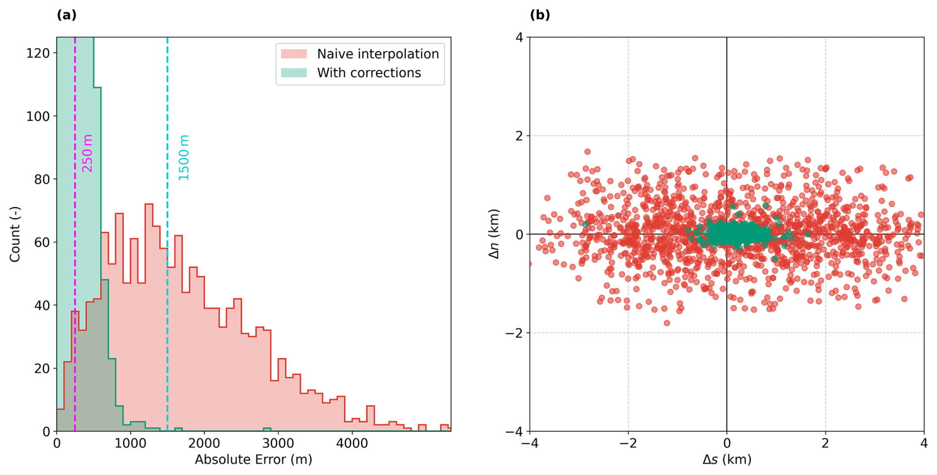
Figure C2 (a) Histogram of collocation errors for naive interpolation (red) and after scanning time and parallax corrections (green). The two vertical dotted lines indicate reference errors for 250 m (magenta) and 1500 m (cyan). (b) Scatterplot showing the errors normal, Δn, and tangential, Δs, to the flight path from the predicted positions to the manually annotated locations. Interpretation of direction of errors can be seen in Fig. 2.

Appendix D: Sample Sentinel-2 and Landsat imagery

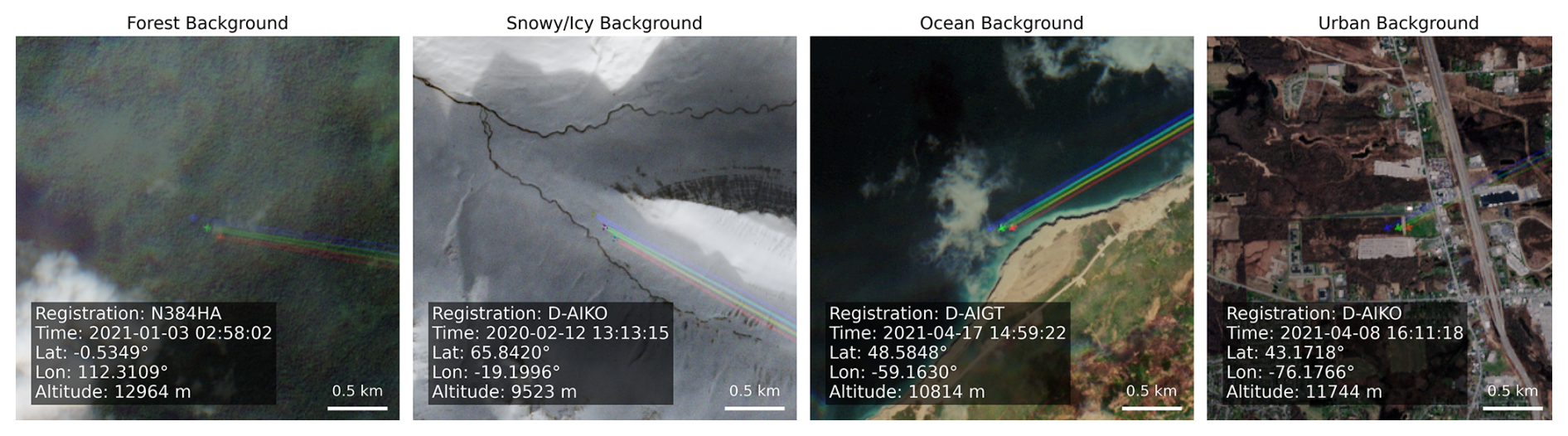
Figure D1 Examples of contrail-forming IAGOS aircraft in Sentinel-2 imagery with different background conditions. The aircraft, sensing time, location and altitude, as well as the scale, are provided for each example. Figures contain modified Copernicus Sentinel data 2020–2021.

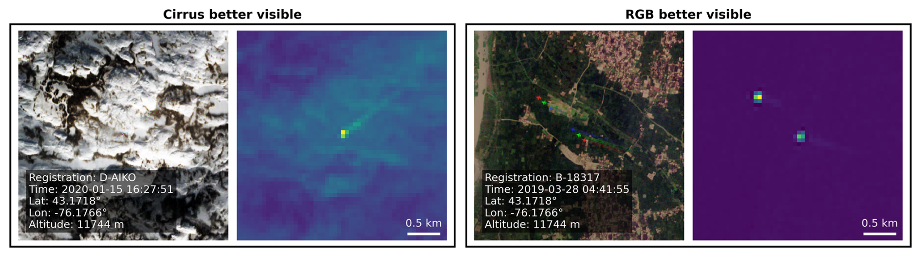
Figure D2 Sentinel-2 collocations comparing the visibility of contrails in true colour and cirrus band images. All images are displayed at the same scale. Note that the example on the right features the same aircraft twice, an artifact caused by the Sentinel-2 detector borders. Figures contain modified Copernicus Sentinel data 2019–2020.

Figure D3 Contrail observed in Sentinel-2 imagery illustrating the occurrence of the Crow instability (Crow, 1970). Contains modified Copernicus Sentinel data 2018.

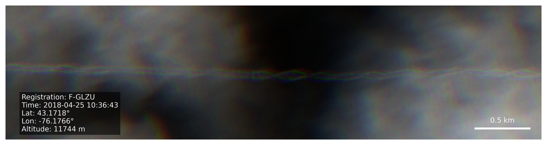
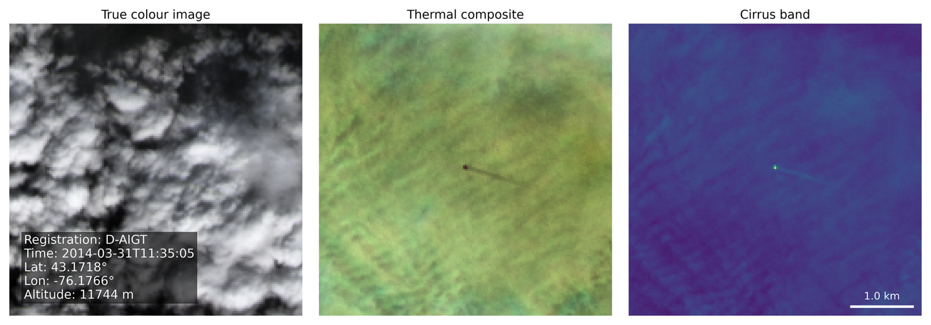
Figure D4 Landsat collocation comparing the visibility of a contrail in the true colour image, false colour composite based on infrared bands, and monochromatic cirrus band image. All images are displayed at the same scale. Landsat-8 image courtesy of the U.S. Geological Survey.