Comparison of tomographic wind retrievals with different geometric implementations for multistatic meteor radar networks

A growing number of multistatic meteor radar networks are being established worldwide. The multistatic geometry with overlapping observation volumes of several meteor radars or passive receivers permits the inference of higher-order kinematic properties of the wind field or even the retrieval of arbitrary wind fields using tomographic algorithms. Furthermore, there is the long-standing question of the reliability of the vertical wind. In this study, we present a novel Volume Velocity Processing in spherical coordinates and perform an initial cross-comparison to previous implementations of the Volume Velocity Processing and the advanced 3DVAR+DIV retrieval. We performed a detailed climatological and multiyear comparison of mean winds, horizontal divergence, relative vorticity, stretching, and shearing deformation using observations of the Nordic Meteor Radar Cluster consisting of the meteor radars at Tromsø, Alta, Kiruna, and Sodankylä. Our results underscore that the spherical implementation of Volume Velocity Processing reduces/minimizes altitude-dependent biases caused by projection errors resulting from an incomplete representation of the observation geometry in the mean horizontal and vertical winds. All algorithms exhibit a very high correlation for the mean horizontal winds, but we found substantial differences in the vertical wind velocity and in the higher-order kinematic properties between the novel algorithm and previous versions of the Volume Velocity Processing. Furthermore, the novel algorithm reproduces a consistent seasonal pattern of the vertical velocity with upwelling during the hemispheric summer at the altitude of the zonal wind reversal and a corresponding but weaker downwelling during the winter months. The magnitudes of the vertical wind appear to be physically consistent with theoretically expected upward and downward motions and are on the order of a few cm s⁻¹. We also identified a scaling effect of the vertical wind in dependence on the temporal resolution and spatial averaging represented by a circle of influence in the new retrieval, which was confirmed by the measurement response of the 3DVAR+DIV retrieval. Wind data retrieved from SSVP and VVP are compared with the Japanese meteorological reanalysis known as JAWARA and SE-WACCM-X model data. The vertical wind patterns observed by the Nordic Meteor Radar Cluster show strong agreement between the two. Robust vertical wind retrievals obtained with a temporal resolution of 15–30 min and within a spatial domain of approximately 200–250 km centered between all meteor radars provide the best compromise between sampling density and spatial averaging for the Nordic Meteor Radar Cluster.

1 Introduction

The mesosphere and lower thermosphere (MLT) cover altitudes of approximately 70–120 km and serve as a key transitional region between the upper and middle atmosphere, which is influenced by forces from above, such as high-energy inputs from solar radiation, and from below through atmospheric waves (Liu, 2016; Plane et al., 2023). This region exhibits complex spatiotemporal dynamics primarily driven by atmospheric waves with different spatiotemporal scales, including gravity waves, tides, planetary waves, quasi-biennial oscillations, and interannual differences, that contribute to the variability in the lower region of the upper atmosphere. These phenomena are crucial for understanding the general circulation of the atmosphere, as the propagation and dissipation of these waves transport energy and momentum horizontally and vertically (Lindzen, 1981). The vertical coupling between the lower, middle, and upper atmosphere is strongly influenced by the prevailing wind fields, underscoring the importance of understanding the wind fields in the middle atmosphere (Fritts et al., 2002; Andrews et al., 1987). A comprehensive understanding of the MLT is essential to elucidate the wave-driven forcing of the upper atmosphere and the corresponding energy exchange between the upper and middle atmospheres. This wave-driven vertical coupling results in the cold summer mesopause temperatures, which can drop below 140 K at high latitudes, making the summer MLT the coldest place on Earth. The summer MLT deviates up to 100 K from the radiatively determined equilibrium temperature (Becker, 2012; Smith, 2012).

Meteoroids are extraterrestrial particles of cometary, asteroidal, or metallic composition that occasionally enter planetary atmospheres (Vondrak et al., 2008; Janches et al., 2009; Dawkins et al., 2023a). Upon entry, they are referred to as meteors. As they penetrate the atmosphere, they produce an ionized trail due to frictional heating, a phenomenon known as meteor ablation in the MLT. The capability of meteor radars to detect specular or transverse scatter reflections from meteor trails enables continuous monitoring of the MLT, allowing for measurement of various atmospheric and meteor-related parameters, including mean winds and wind fluctuations (momentum flux), neutral air density variability, temperature, and pressure, as well as all parameters associated with the meteoroid origin such as the velocity, mass and source radiant (see e.g., Manning et al., 2006; Hook, 1970; Holdsworth et al., 2004; Fritts et al., 2010; Hocking et al., 2001; de Wit et al., 2014; Yi et al., 2019; Hall and Tsutsumi, 2020; Wilhelm et al., 2019; Kozlovsky et al., 2025; Hindley et al., 2022; Reid, 2024; Stober et al., 2012b; Dawkins et al., 2023b; He et al., 2024; Dawkins et al., 2023a, among others).

During the past decades, Meteor radars have evolved into reliable and robust instruments for atmospheric measurements at the MLT, capable of continuous, automated, and remote operations, functioning uninterrupted as long as a power supply is available, regardless of weather conditions. A typical monostatic meteor radar measures horizontal winds with a temporal resolution of about 1 h, based on a limited number of meteor detections. However, increasing the number of meteors detected within a given spatial volume and time interval improves both accuracy and resolution of the wind measurement, as achieved with multistatic meteor radar networks. Such multistatic meteor radar networks can achieve temporal resolutions of a few minutes (Stober et al., 2023; Qiao et al., 2025).

Over the past five years, several multistatic meteor radar networks have become operational, offering an unprecedented opportunity for observing atmospheric dynamics in three dimensions. These multistatic systems enable the observation of a standard atmospheric volume, which is ideal for inferring the spatial variability of three-dimensional (3D) winds by utilizing advanced statistical inversion methods and tomographic approaches, such as algebraic least squares fits based on the Volume Velocity Processing (VVP) introduced by Waldteufel and Corbin (1979), which was later applied in various studies (e.g., Stober and Chau, 2015; Chau et al., 2017; Conte et al., 2025; Zeng et al., 2024) and more sophisticated Bayesian approaches such as the 3DVAR+DIV retrieval algorithms (Stober et al., 2021a, 2022; Qiao et al., 2025; Kozlovsky et al., 2025), other Bayesian implementations (Volz et al., 2021) or machine learning (Urco et al., 2024).

The Volume Velocity Processing (VVP) retrieval method is an advancement of the earlier so-called Velocity Azimuth Display (VAD) method (Browning and Wexler, 1968). Both approaches apply an appropriate fitting procedure to infer mean winds and to obtain a first-order approximation of the spatial variability of the flow field, under the assumption that these inhomogeneities can be linearly approximated (Browning and Wexler, 1968; Waldteufel and Corbin, 1979; Stober and Chau, 2015; Zeng et al., 2024). However, when the MLT winds are assumed to be arbitrary, this method encounters a limitation that can be overcome using the three-dimensional variational (3DVAR) algorithm implemented as part of the Agile Software for Gravity wAve Regional Dynamics (ASGARD) framework, demonstrating that non-linear error propagation, Gaussian weighting, and smoothness regularization can be applied to derive horizontal wind components (Stober et al., 2021a). The 3DVAR resolves 3D wind fields across all grid cells, incorporating variable geographic and Cartesian coordinate grids. The 3DVAR+DIV method is an advancement of the 3DVAR algorithm (Stober et al., 2022, 2023; Qiao et al., 2025), combining the radial velocity observations with the continuity equation. This method represents a transition from purely observation-driven parameter estimation to more physics- and model-based data analysis.

In this study, we present statistics from the Nordic Meteor Radar Cluster (NORDIC) observations covering the period from January 2021–June 2025, along with a Spherical Velocity Volume Processing (SVVP) method based on spherical geometry and a first-order approximation of the ellipsoidal shape of our Earth. We developed this novel algorithm to reduce biases in the estimated vertical winds, which are crucial for inferring reliable momentum fluxes and assessing the mean vertical motion due to the residual circulation. The SVVP algorithm targets the need for a computationally less expensive tomographic algorithm ideal for deriving climatologies or long time series of mean winds and first-order approximations of the wind field within a defined geographic domain, such as horizontal divergence, relative vorticity, stretching, and shearing deformation. We compare the newly developed SVVP with a previous VVP routine to highlight the importance of spherical geometry on derived parameters, including mean 3D winds, horizontal divergence, relative vorticity, stretching, and shearing deformation. We also perform a comparison to the Bayesian 3DVAR+DIV retrieval algorithm to investigate the temporal and spatial variability of the three-dimensional wind field in the MLT. The comparison focuses on statistical analyses, including an initial assessment of vertical winds, which are constrained by the continuity equation and horizontal divergence. This paper is structured as follows. In Sect. 2, we present the data description and statistical overview. Section 3 introduces the Volume velocity Processing on a sphere. Section 4 presents the error analysis and numerical robustness. Section 5 presents the results of wind climatology and statistical analysis. Section 6 provides the discussion. Finally, Sect. 7 summarizes our conclusions. We also provide supplementary material containing additional results for all radii and temporal scales of the VVP analysis.

2 Nordic Meteor Radar Cluster

In this study, we utilize observations from the Nordic Meteor Radar Cluster (NORDIC). A multistatic radar network of meteor radars located across Northern Scandinavia that consists of five monostatic meteor radars namely, Tromsø (69.59° N, 19.2° E; TRO), Alta (70.0° N, 23.3° E; ALT), Sodankylä (67.4° N, 26.6° E; SOD), Kiruna (67.9° N, 21.1° E; KIR), Svalbard (78.2° N, 16.0° E; SVA). However, for this study, we only use the mainland systems, and the Svalbard meteor radar was omitted. The period that is analyzed spans from January 2021–June 2025. Figure 1 and Table 1 illustrate the geographical locations of the four meteor radar stations and the technical parameters of the NORDIC Meteor Radar Cluster.

Table 1 Operational Parameters of the NORDIC Meteor Radar Cluster network. PRF describes the Pulse Repetition Frequency. The MR located at Kiruna was updated on 18 March 2024 and has been operating with new experiment parameters since then. In September 2009, the Sodankylä MR was upgraded to a 15 kW transmitter.

Figure 1 Nordic Meteor Radar Cluster locations at TRO, ALT, KIR, and SOD (red dots). The plot is generated with etopo1 using the m_map package (Amante and Eakins, 2009).

Figure 2 presents the two-dimensional (2D) horizontal distribution of meteors detected by the radar stations (indicated by color-coded dots) recorded over three days (1–3 April 2021), along with the altitude distribution for the entire study period. The scatter plot on the map illustrates the spatial distribution of meteor echoes, with colors representing the meteor echoes for each station: blue for Tromsø, purple for Alta, cyan for Kiruna, and magenta for Sodankylä. The stations exhibit overlapping coverage regions, with TRO, ALT, and KIR showing substantial overlap with each other compared to SOD, although SOD partially overlaps with KIR. The altitude distributions approximately show a Gaussian profile within the altitude range of 70–120 km, peaking around 90 km for all stations, with median altitudes of 90.8 km for TRO, 91.2 km for ALT, 90.0 km for KIR, and 89.6 km for SOD. Among all the stations, it is observed that the Alta radar station detected the highest meteor count, followed by Tromsø, Sodankylä, and Kiruna.

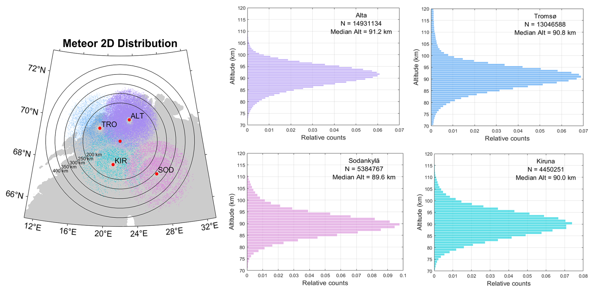
Figure 2 The 2D Horizontal distribution of meteor positions detected by the meteor radar stations (indicated with color-coded dots) from 1–3 April 2021, with each point representing a detected meteor. Red dots indicate station locations, with their labels identifying each station; the unlabeled dot marks the central reference point used for the SVVP retrievals. The concentric rings represent distance in km from this central reference point. The altitude distribution of meteors detected at each station is also shown, indicating the total number of meteors observed during the study period (January 2021–June 2025) and the corresponding median altitude for each station. The colors blue, Cyan, purple, and magenta correspond to meteors detected at TRO, ALT, KIR, and SOD stations, respectively.

The altitudinal profile of the long-term changes in the detected meteor echo rates for all stations during the study period, along with the hourly distribution of meteors for 3 d (1–3 April), is illustrated in Fig. 3. A distinct inter-annual variation pattern is revealed, with a pronounced change in the number of meteor echoes with altitude and season. Meteor echoes are detected between the altitudes of 82 and 95 km and during the summer months for all the radar stations. The white lines represent gaps in the measurements of a system. In particular, the update in Kiruna in 2024 resulted in a gap, and a second gap occurred in 2025. The temporal distributions of selected days exhibit a similar trend, showing a diurnal variation, reaching maximum values in the morning (08:00–10:00 UTC) and minimum values in the evening (17:00–19:00 UTC).

The wind components in the MLT region are obtained using the 3DVAR+DIV algorithm with geographic grid coordinates (Stober et al., 2022), VVP, and the novel spherical VVP algorithm described in the next section. The retrievals have temporal resolutions of 15 min, 30 min, and 1 h, covering altitudes from 70–110 km with a vertical resolution of 2 km. The horizontal domain (radius) implemented in the new spherical VVP (SVVP) and VVP algorithm was varied from 200–400 km in steps of 50 km. Unless otherwise specified, the reference results presented in this study correspond to the 250 km horizontal domain for the VVP/SVVP method and a 30 min temporal resolution for both algorithms. For the 3DVAR+DIV retrievals, the Tikhonov regularization parameter (α) of 0.4 and 150 was used to assess their impact on the derived wind fields. The complete set of results is presented as Supplementary material.

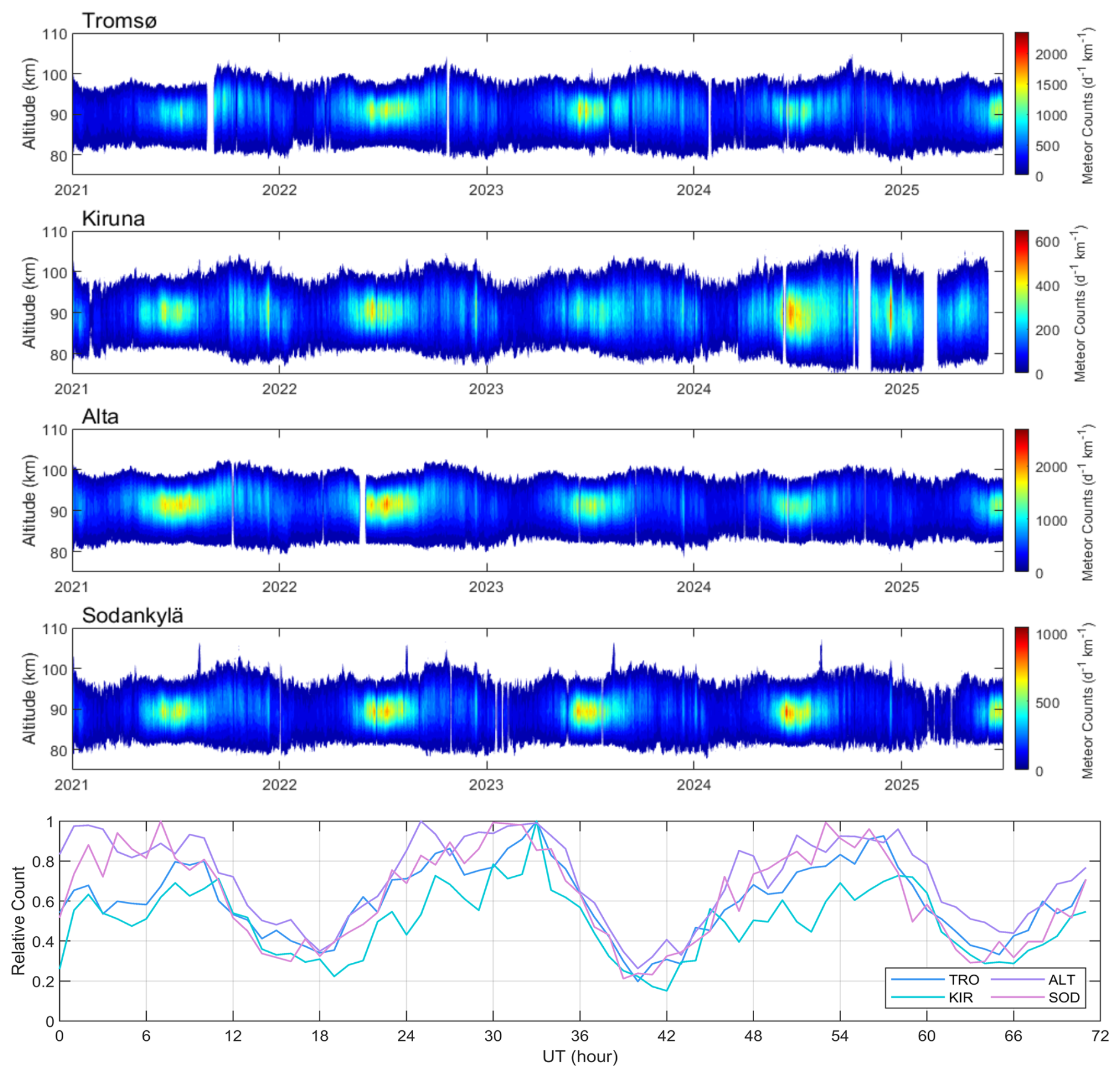
Figure 3 Altitudinal profile of daily meteor echoes detected by all four meteor radars. The lower stair-step diagram illustrates the hourly temporal distribution of meteors from 1–3 April 2021. The four colors have the same meaning as in the previous figure.

In addition, we employ the JAGUAR-DAS whole neutral atmosphere reanalysis (JAWARA) data produced by the Japanese Atmospheric General Circulation Model for Upper Atmosphere Research-Data Assimilation System (JAGUAR-DAS) (Koshin et al., 2020, 2022, 2025) and the SE-WACCM-X version of the Whole Atmosphere Community Climate Model with thermosphere/ionosphere extension (WACCM-X) model (Liu et al., 2018, 2024; Lauritzen et al., 2018; Liu, 2025) for comparison with the SVVP and VVP output. Both datasets were extracted for the same longitude and latitude as the NORDIC Cluster and matched the altitude range for the VVP and SVVP Model output, as well as the time span of the data used in this study.

3 Derivation of Volume Velocity Processing on a Sphere

Over the past decade, Volume Velocity Processing (VVP) has become a more commonly used approach to assess spatial wind variability in multistatic meteor radar observations (Stober et al., 2013; Stober and Chau, 2015; Chau et al., 2017; Zeng et al., 2024). Additionally, the basic idea of the VVP remains consistent with the original publications from Browning and Wexler (1968); Waldteufel and Corbin (1979). However, the implementation of the algorithm can become more complicated when describing larger domain areas (Stober et al., 2021a; Qiao et al., 2025; Zeng et al., 2024, 2026; Ban et al., 2026; Yi et al., 2026), which can extend horizontally to several hundred kilometers. Here, we will outline the most recent version of our VVP implementation. The revised version builds on previous developments presented in Zeng et al. (2024), but is now generalized to spherical coordinates and incorporates higher-order corrections to account for the ellipsoidal shape of the Earth, and not only considers the WGS84 model for each measurement, but also the spherical geometry for the observation volume.

Recalling the original form of the VVP for plane geometry presented in Waldteufel and Corbin (1979), we can express the wind field by a Taylor expansion consisting of mean zonal, meridional, and vertical wind components and first-order deviations given by linear spatial derivatives;

$$\begin{array}{ll}\text{(1)}& {\displaystyle }u(x,y)& {\displaystyle }=u_{\mathrm{0}}(x_{\mathrm{0}},y_{\mathrm{0}})+{\displaystyle \frac{\partial u}{\partial x}}\cdot \mathrm{\Delta }x+{\displaystyle \frac{\partial u}{\partial y}}\cdot \mathrm{\Delta }y{\displaystyle }v(x,y)& {\displaystyle }=v_{\mathrm{0}}(x_{\mathrm{0}},y_{\mathrm{0}})+{\displaystyle \frac{\partial v}{\partial x}}\cdot \mathrm{\Delta }x+{\displaystyle \frac{\partial v}{\partial y}}\cdot \mathrm{\Delta }y\\ {\displaystyle }w(x,y)& {\displaystyle }=w_{\mathrm{0}}(x_{\mathrm{0}},y_{\mathrm{0}}).\end{array}$$

Here u, v, and w correspond to the zonal, meridional, and vertical wind components, respectively. The vertical wind is defined in the ENU (East-North-Up) direction above the WGS84 ellipsoid for the reference coordinate. The quantity represents the vertical motion of the entire cone segment spanned by the circle of influence and the width of the vertical layer (2 km default). The subscript 0 indicates the domain reference coordinate (x₀,y₀), which is a free parameter that can be arbitrarily selected. However, it turns out that the domain center appears to be a good choice. Thus, $\mathrm{\Delta }x=x-x_{\mathrm{0}}$ and $\mathrm{\Delta }y=y-y_{\mathrm{0}}$ measure the distance to any coordinate (x,y).

After a mathematical expansion and rearranging the horizontal derivatives, the first-order kinematic inhomogeneities of any linear or non-linear wind field can be approximated by the horizontal divergence, the relative vorticity, and the stretching and shearing deformation;

$$\begin{array}{rl}u=& u_{\mathrm{0}}+{\displaystyle \frac{\mathrm{1}}{\mathrm{2}}}\underset{\text{hor. divergence}}{\underbrace{\left({\displaystyle \frac{\partial u}{\partial x}}+{\displaystyle \frac{\partial v}{\partial y}}\right)}}\cdot \mathrm{\Delta }x-{\displaystyle \frac{\mathrm{1}}{\mathrm{2}}}\underset{\text{rel. vorticity}}{\underbrace{\left({\displaystyle \frac{\partial v}{\partial x}}-{\displaystyle \frac{\partial u}{\partial y}}\right)}}\cdot \mathrm{\Delta }y\\ & +{\displaystyle \frac{\mathrm{1}}{\mathrm{2}}}\underset{\text{stretching def.}}{\underbrace{\left({\displaystyle \frac{\partial u}{\partial x}}-{\displaystyle \frac{\partial v}{\partial y}}\right)}}\cdot \mathrm{\Delta }x+{\displaystyle \frac{\mathrm{1}}{\mathrm{2}}}\underset{\text{shearing def.}}{\underbrace{\left({\displaystyle \frac{\partial v}{\partial x}}+{\displaystyle \frac{\partial u}{\partial y}}\right)}}\cdot \mathrm{\Delta }y\end{array}$$

$$\begin{array}{}\text{(2)}& \begin{array}{rl}v=& v_{\mathrm{0}}+{\displaystyle \frac{\mathrm{1}}{\mathrm{2}}}\underset{\text{hor. divergence}}{\underbrace{\left({\displaystyle \frac{\partial u}{\partial x}}+{\displaystyle \frac{\partial v}{\partial y}}\right)}}\cdot \mathrm{\Delta }y+{\displaystyle \frac{\mathrm{1}}{\mathrm{2}}}\underset{\text{rel. vorticity}}{\underbrace{\left({\displaystyle \frac{\partial v}{\partial x}}-{\displaystyle \frac{\partial u}{\partial y}}\right)}}\cdot \mathrm{\Delta }x\\ & -{\displaystyle \frac{\mathrm{1}}{\mathrm{2}}}\underset{\text{stretching def.}}{\underbrace{\left({\displaystyle \frac{\partial u}{\partial x}}-{\displaystyle \frac{\partial v}{\partial y}}\right)}}\cdot \mathrm{\Delta }y+{\displaystyle \frac{\mathrm{1}}{\mathrm{2}}}\underset{\text{shearing def.}}{\underbrace{\left({\displaystyle \frac{\partial v}{\partial x}}+{\displaystyle \frac{\partial u}{\partial y}}\right)}}\cdot \mathrm{\Delta }x.\end{array}\end{array}$$

The advantage of these higher-order kinematic terms is that they can be linked to other dynamic parameters, which are more intuitive for dynamic flow fields than the spatial derivatives alone. Furthermore, horizontal divergence is related to the vertical velocity, which is often more difficult to measure. Assuming incompressibility of the atmosphere permits reducing the continuity equation to the following expression (Stober et al., 2022);

$$\begin{array}{}\text{(3)}& \text{div}\left(\mathbf{\text{u}}\right)={\displaystyle \frac{\partial u}{\partial x}}+{\displaystyle \frac{\partial v}{\partial y}}+{\displaystyle \frac{\partial w}{\partial z}}=\mathrm{0}.\end{array}$$

The change in the vertical velocity Δw between two layers can then be derived by vertical integration of the horizontal divergence;

$$\begin{array}{}\text{(4)}& \mathrm{\Delta }w=\underset{z_{\mathrm{1}}}{\overset{z_{\mathrm{2}}}{\int }}\text{div}\cdot v_h\mathrm{d}z.\end{array}$$

This vertical velocity profile depends on the boundary condition of the integral, which has to be determined separately. However, the method was often implemented for the data analysis of meteorological wind profilers in the troposphere. In these cases, the initial surface boundary condition for the vertical wind is zero. Furthermore, the Cartesian coordinates and plane geometry are sufficiently accurate for the small measurement domains typically covered by wind profilers, allowing for the reliable measurement of horizontal divergence and, thus, the inference of vertical winds.

However, multistatic meteor radar networks cover much larger domain areas extending over hundreds of kilometers, and, therefore, it is crucial to consider and represent the Earth's ellipsoidal geometry in the retrievals (Stober et al., 2018, 2021a). In particular, vertical winds are very sensitive to projection errors. Tomographic retrievals, such as the 3DVAR and 3DVAR+DIV algorithms, approximate the Earth's ellipsoid shape by the World Geodetic System 84 (WGS84) reference ellipsoid (National Imagery and Mapping Agency, 2000). The horizontal divergence is inferred by calculating the distance between grid cells in zonal and meridional directions to estimate the spatial derivatives, accounting for the change in the Earth's radius with latitude. A similar method was implemented in a revised VVP algorithm dedicated to larger domain meteor radar networks presented in Zeng et al. (2024, 2026); Ban et al. (2026). Including the WGS84 geometry seems to be reliable up to scales of a few tens of kilometers. However, for much larger domains, the horizontal divergence and, thus, the vertical velocity, tend to produce more spurious results.

Here, we introduce a new VVP based on local spherical coordinates to account for the latitude-dependent change of the Earth's radius. In contrast to previous routines, we outline in detail the basic steps and derive the key transformations that facilitate a comparison with the kinematic terms expressed in Cartesian coordinates, as shown in Eq. 2. Coordinates on a sphere are defined by a radius r, an azimuth ϕ, and a colatitude from the North Pole $\mathit{\theta }=\mathrm{90}\mathit{°}-\mathrm{\Phi }$ for a given latitude Φ. For all further derivations, we will keep the mathematical convention. Furthermore, we define the zonal and meridional wind components as $\dot{\mathit{\varphi }}$ and $\dot{\mathit{\theta }}$, respectively. The vertical velocity is given by $\dot{r}$. The conversion to the well-known Cartesian vector winds in the ENU (East-North-Up) frame of reference is given by;

$$\begin{array}{}\text{(5)}& \begin{array}{rl}u& =r\sin \mathit{\theta }\dot{\mathit{\varphi }}\\ v& =-r\dot{\mathit{\theta }}\\ w& =\dot{r}\end{array}\end{array}$$

Furthermore, we need to transform the spatial derivatives into spherical coordinates. It is worth noting that the derivative also acts on the basis vectors. Recalling that a geometric object (vector) is independent of the coordinate system, leading to the identity for any given wind vector in the form;

$$\begin{array}{}\text{(6)}& u\cdot e_x+v\cdot e_y+w\cdot e_z=\mathbf{\text{u}}=\dot{r}\cdot e_r-r\dot{\mathit{\theta }}\cdot e_{\mathit{\theta }}+\sin \mathit{\theta }r\dot{\mathit{\varphi }}\cdot e_{\mathit{\varphi }}.\end{array}$$

Here, $(e_x,e_y,e_z)$ is the basis vector in Cartesian coordinates and $(e_r,e_{\mathit{\theta }},e_{\mathit{\varphi }})$ denotes the basis vector in spherical coordinates. Considering the additional contributions of the derivatives due to the basis vectors, we can write the spatial derivative terms of our wind vector in spherical coordinates as;

$$\begin{array}{}\text{(7)}& {\displaystyle \frac{\partial u}{\partial x}}\cdot e_x& {\displaystyle }={\displaystyle \frac{\partial \dot{\mathit{\varphi }}}{\partial \mathit{\varphi }}}\cdot e_{\mathit{\varphi }}\text{(8)}& {\displaystyle \frac{\partial u}{\partial y}}\cdot e_y& {\displaystyle }=(\mathrm{2}\dot{\mathit{\varphi }}\cdot \cos \mathit{\theta }+\sin \mathit{\theta }\cdot {\displaystyle \frac{\partial \dot{\mathit{\varphi }}}{\partial \mathit{\theta }}})\cdot e_{\mathit{\theta }}\text{(9)}& {\displaystyle \frac{\partial v}{\partial x}}\cdot e_x& {\displaystyle }=-{\displaystyle \frac{\mathrm{1}}{\sin \mathit{\theta }}}{\displaystyle \frac{\partial \dot{\mathit{\theta }}}{\partial \mathit{\varphi }}}\cdot e_{\mathit{\varphi }}\text{(10)}& {\displaystyle \frac{\partial v}{\partial y}}\cdot e_y& {\displaystyle }=(-{\displaystyle \frac{\partial \dot{\mathit{\theta }}}{\partial \mathit{\theta }}}-\dot{\mathit{\theta }}\cdot \cot \mathit{\theta })\cdot e_{\mathit{\theta }}\end{array}$$

Furthermore, the Δx and Δy terms have to be expressed in spherical geometry as well. We calculate the distance of the arc-segment between two geographic points using the WGS84 reference ellipsoid as implemented in Zeng et al. (2024);

$$\begin{array}{}\text{(11)}& \begin{array}{rl}\mathrm{\Delta }x& =r_{\mathrm{m}}\cdot \sin {\mathit{\theta }}_{\mathrm{m}}\mathrm{\Delta }\mathit{\varphi }=r_{\mathrm{m}}\sin {\mathit{\theta }}_{\mathrm{m}}(\mathit{\varphi }-{\mathit{\varphi }}_{\mathrm{0}})\\ \mathrm{\Delta }y& =r_{\mathrm{m}}\mathrm{\Delta }\mathit{\theta }=r_{\mathrm{m}}(\mathit{\theta }-{\mathit{\theta }}_{\mathrm{0}})\end{array}\end{array}$$

Here r_m and θ_m denote the mean Earth radius and mean zenith distance considering the reference geographic location in spherical coordinates (ϕ₀,θ₀) and any other geographic position expressed in zenith distance/co-latitude (ϕ,θ) (mathematical convention). These coordinates are related to the well-known geographic latitude by $\mathrm{\Phi }=\mathrm{90}-\mathit{\theta }$ and ϕ corresponds to the longitude λ. We can now rewrite Eq. (1) in spherical coordinates and approximate the ENU vector wind $(u,v,w)$ at geographic coordinates (long, lat) by the following set of equations;

$$\begin{array}{}\text{(12)}& \begin{array}{rl}u(\mathit{\lambda },\mathrm{\Phi })& =u_{\mathrm{0}}({\mathit{\lambda }}_{\mathrm{0}},{\mathrm{\Phi }}_{\mathrm{0}})+{\displaystyle \frac{\partial \dot{\mathit{\varphi }}}{\partial \mathit{\varphi }}}{r}_{\mathrm{m}}\sin {\mathit{\theta }}_{\mathrm{m}}\mathrm{\Delta }\mathit{\varphi }\\ & -\sin {\mathit{\theta }}_{\mathrm{0}}\cdot {\displaystyle \frac{\partial \dot{\mathit{\varphi }}}{\partial \mathit{\theta }}}{r}_{\mathrm{m}}\mathrm{\Delta }\mathit{\theta }+\mathrm{2}{u}_{\mathrm{0}}\cdot {\displaystyle \frac{\cos {\mathit{\theta }}_{\mathrm{0}}}{r_{\mathrm{0}}\sin {\mathit{\theta }}_{\mathrm{0}}}}{r}_{\mathrm{m}}\mathrm{\Delta }\mathit{\theta }\\ v(\mathit{\lambda },\mathrm{\Phi })& =v_{\mathrm{0}}({\mathit{\lambda }}_{\mathrm{0}},{\mathrm{\Phi }}_{\mathrm{0}})-{\displaystyle \frac{\mathrm{1}}{\sin {\mathit{\theta }}_{\mathrm{0}}}}{\displaystyle \frac{\partial \dot{\mathit{\theta }}}{\partial \mathit{\varphi }}}{r}_{\mathrm{m}}\sin {\mathit{\theta }}_{\mathrm{m}}\mathrm{\Delta }\mathit{\varphi }\\ & +{\displaystyle \frac{\partial \dot{\mathit{\theta }}}{\partial \mathit{\theta }}}{r}_{\mathrm{m}}\mathrm{\Delta }\mathit{\theta }+v_{\mathrm{0}}\cdot {\displaystyle \frac{\cot {\mathit{\theta }}_{\mathrm{0}}}{r_{\mathrm{0}}}}{r}_{\mathrm{m}}\mathrm{\Delta }\mathit{\theta }\\ w(\mathit{\lambda },\mathrm{\Phi })& =w({\mathit{\lambda }}_{\mathrm{0}},{\mathrm{\Phi }}_{\mathrm{0}}).\end{array}\end{array}$$

Here, we have already introduced some additional sign conventions. The colatitude is defined with the opposite sign compared to the meridional wind, and we replaced the angular velocity with the 3D Cartesian local vector winds in the ENU frame of reference. This step is not trivial, and we cross-checked all terms by comparing them to the standard VVP and by performing the derivation in latitudinal spherical coordinates. Transforming the VVP from Cartesian into spherical coordinates, which are more appropriate for the larger domain size typically covered by multistatic meteor radar networks, results in additional terms. The mean winds have an additional contribution due to the latitudinal extent of the observational domain. The resulting set of equations using latitude as a reference is given in Appendix A. The meridional spatial derivatives for the zonal and meridional gradients depend on the mean zonal and meridional wind as well. The above-presented solutions apply to meteor radar networks at high, mid-, and low latitudes in the Northern and Southern hemispheres. However, there is a singular term in the meridional wind equation that results in two singularities, one at each pole. From Eq. (12), we can also calculate the corresponding expression of the horizontal divergence (∇_hu) and relative vorticity (∇×u)_r in spherical coordinates;

$$\begin{array}{}\text{(13)}& {\displaystyle }& {\displaystyle }{\displaystyle }({\displaystyle \frac{\partial u}{\partial x}}+{\displaystyle \frac{\partial v}{\partial y}})={\mathrm{\nabla }}_{\mathrm{h}}\cdot \mathbf{\text{u}}=({\displaystyle \frac{\partial \dot{\mathit{\varphi }}}{\partial \mathit{\varphi }}}+{\displaystyle \frac{\partial \dot{\mathit{\theta }}}{\partial \mathit{\theta }}}-v_{\mathrm{0}}\cdot {\displaystyle \frac{\cot \mathit{\theta }}{r_{\mathrm{0}}}})\text{(14)}& {\displaystyle }& {\displaystyle }\begin{array}{rl}{\displaystyle }& {\displaystyle }({\displaystyle \frac{\partial v}{\partial x}}-{\displaystyle \frac{\partial u}{\partial y}})=(\mathrm{\nabla }\times \mathbf{\text{u}}{)}_r=\\ {\displaystyle }& {\displaystyle }({\displaystyle \frac{\mathrm{1}}{\sin \mathit{\theta }}}{\displaystyle \frac{\partial \dot{\mathit{\theta }}}{\partial \mathit{\varphi }}}-\sin \mathit{\theta }\cdot {\displaystyle \frac{\partial \dot{\mathit{\varphi }}}{\partial \mathit{\theta }}}+\mathrm{2}{u}_{\mathrm{0}}\cdot {\displaystyle \frac{\cos \mathit{\theta }}{r_{\mathrm{0}}\sin \mathit{\theta }}}),\end{array}\end{array}$$

and the stretching and shearing deformation;

$$\begin{array}{}\text{(15)}& {\displaystyle }& {\displaystyle }({\displaystyle \frac{\partial u}{\partial x}}-{\displaystyle \frac{\partial v}{\partial y}})=({\displaystyle \frac{\partial \dot{\mathit{\varphi }}}{\partial \mathit{\varphi }}}-{\displaystyle \frac{\partial \dot{\mathit{\theta }}}{\partial \mathit{\theta }}}+v_{\mathrm{0}}\cdot {\displaystyle \frac{\cot \mathit{\theta }}{r_{\mathrm{0}}}})\text{(16)}& {\displaystyle }& {\displaystyle }({\displaystyle \frac{\partial v}{\partial x}}+{\displaystyle \frac{\partial u}{\partial y}})=({\displaystyle \frac{\mathrm{1}}{\sin \mathit{\theta }}}{\displaystyle \frac{\partial \dot{\mathit{\theta }}}{\partial \mathit{\varphi }}}+\sin \mathit{\theta }\cdot {\displaystyle \frac{\partial \dot{\mathit{\varphi }}}{\partial \mathit{\theta }}}-\mathrm{2}{u}_{\mathrm{0}}\cdot {\displaystyle \frac{\cos \mathit{\theta }}{r_{\mathrm{0}}\sin \mathit{\theta }}}).\end{array}$$

Considering that line-of-sight velocities or radial velocities are always measured in the ENU frame of reference for each MR, we implemented a fitting scheme around the variables $u_{\mathrm{0}},v_{\mathrm{0}},w_{\mathrm{0}},\frac{\partial \dot{\mathit{\varphi }}}{\partial \mathit{\varphi }},\frac{\partial \dot{\mathit{\varphi }}}{\partial \mathit{\theta }},\frac{\partial \dot{\mathit{\theta }}}{\partial \mathit{\varphi }}$, and $\frac{\partial \dot{\mathit{\theta }}}{\partial \mathit{\theta }}$ and calculated the higher-order kinematic terms from the obtained coefficients. A crucial aspect of the solver is the dependency of the gradient terms on the mean winds, or that the mean wind also contributes to the gradient. Our choice of the fitting coefficients in spherical coordinates avoids solving a nonlinear problem.

In addition to formulating the mathematical equations in spherical coordinates, we retain nonlinear error propagation for all coefficients and the generalized Tikhonov regularization, which was used in previous implementations (Stober et al., 2022; Zeng et al., 2024; Lieberman et al., 2025). The nonlinear error propagation includes the line-of-sight velocity uncertainty from the recorded data, an angular uncertainty of 2° for the zenith and azimuth angles, and the temporal and spatial shear terms as introduced in Stober et al. (2018), Gudadze et al. (2019), and Hindley et al. (2022). The nonlinear error propagation is solved iteratively, as the mean wind directly scales the angular uncertainties. We apply up to 8 iterations to obtain a stable solution for the VVP and SVVP. More details are provided in Appendix B.

The Tikhonov regularization also remains valid for the spherical-coordinate implementation in obtaining reliable vertical velocities. We calculate a predictor from the grid cells above and below a reference coordinate in altitude as well as in time, using a time step before and after. This regularization approach helps to cure ill-conditioned spatial sampling. However, the vertical wind shows a much better agreement between the direct Doppler-derived vertical velocity and the horizontal divergence-inferred vertical wind, providing confidence in the overall reliability of the implementation. The climatologies and long-term measurements presented in the results section are based on the Doppler-derived measurements, as a detailed analysis of the divergence-estimated vertical winds is beyond the scope of this paper. The divergence-estimated vertical winds require a lower or upper integration boundary, which is not straightforward to implement.

4 Error analysis and numerical robustness

We also determine a mean seasonal or long-term vertical wind bias based on the considerations presented in Rodgers (2000). The underlying assumption is that multi-year or long-term vertical winds should have a vanishing mean. Considering that even a mean deviation in the vertical wind of 1 mm s⁻¹ over one year would result in enormous vertical motions of 31 km yr⁻¹. Such large vertical motions of air packages are not observed nor predicted by GCMs. In this study, we estimated the bias from even longer time series. Typical bias values are calculated for each altitude and range from 1–8 cm s⁻¹ and are subtracted to obtain the vertical wind speeds shown in the climatology and multi-year data. The altitude-dependent bias is estimated from;

$$\begin{array}{}\text{(17)}& w_{\text{bias}}\left(z\right)={\displaystyle \frac{\mathrm{1}}{N}}\sum _{t}w(z,t),\end{array}$$

and subtracted from each altitude separately. In addition, we estimate the standard deviation, which corresponds more to the variability of the vertical wind rather than a statistical uncertainty of the mean. Furthermore, we can justify our bias correction by considering previous results. The most precise and accurate measurements of the vertical motion of the meteor layer are obtained by tracking the mean ablation altitude (Stober et al., 2014; Dawkins et al., 2023b). These studies suggest that the middle atmosphere is shrinking by a maximum of 850 m per decade. This translates to a mean vertical velocity of $\mathrm{2.6}\times {\mathrm{10}}^{-\mathrm{6}}\mathrm{m}{\mathrm{s}}^{-\mathrm{1}}$. Thus, it is reasonable to consider any substantial deviation from this value over a period of 5 years or from the climatological mean at each altitude as bias, which can be subtracted. This method is valid under the assumptions that the radars retain a constant sensitivity and that the statistical properties of the sporadic meteoroid population have no significant trend concerning the chemical composition, velocity, or mass of the meteoroids.

The bias correction is also more relevant for the Doppler-derived vertical velocity, which directly depends on the pointing accuracy. Considering typical wind speeds ranging from 10–100 m s⁻¹ (planetary waves + tides + gravity waves) would introduce a vertical velocity of a few cm s⁻¹, assuming a pointing error of 0.1°. However, each system likely has an uncorrelated pointing error compared to the other radars in the network. Currently, we estimate an average difference in the source radiant position for different meteor showers (data not shown) of ±0.5° between the systems, which falls into the range of the applied bias correction.

Figure 4 Vertical wind bias at 15 and 30 min temporal resolutions for 200 and 250 km is shown in panels (a, b), respectively. For comparison, panel (c) presents the normalized altitude distribution, serving as a proxy for the measurement statistics. The displayed errors denote the standard deviation of the climatology, which is also representative of the 5 year series.

SVVP retrievals are rather robust for the mean winds $(u,v,w)$ concerning the number of radars in the network. There is almost no impact on those parameters when one of the systems is not operating. However, the gradient terms are rather sensitive to missing data in one section of the domain. Tromsø and Alta MR have a substantially higher number of detections (typically twice as many) compared to Kiruna and Sodankylä. As a result, the retrieved quantities require at least three operational radars, including Tromsø and Alta. A leave-one-station-out experiment resulted in a marginal degradation of the vertical wind magnitude comparable to the scaling behaviour between 15 and 30 min temporal resolution (See Supplement).

A more detailed diagnostic comparing planar and spherical geometry can be obtained by looking at the fitting residuals. Figure 5 shows the fitting residuals for two cases. The distance from the zero line of the residuals indicates a deviation from the model assumption. A perfect model would produce residuals with error bars that overlap the zero line. Linear trends or other features, such as a sinusoidal pattern, are often an indication that the model fit is not capturing all the information that is available in the data. The first case (upper panels) shows a typical situation where both fits exhibit a normal distribution around the zero line. However, VVP fits tend to produce more extreme values for some measurements, which mostly vanish in the SVVP implementation. Furthermore, the fitting errors for the mean wind components are often smaller using the SVVP geometry compared to the planar fit. The remaining standard deviation reflects the small-scale fluctuation inside the circle of influence, which is resolved by the 3DVAR+DIV, but acts as a noise source for the VVP and SVVP. As the standard deviation between VVP and SVVP exhibits only small differences, the overall errors are very similar for both model fits. The lower two panels c) and d) highlight a case where the first-order wind field approximation fails.

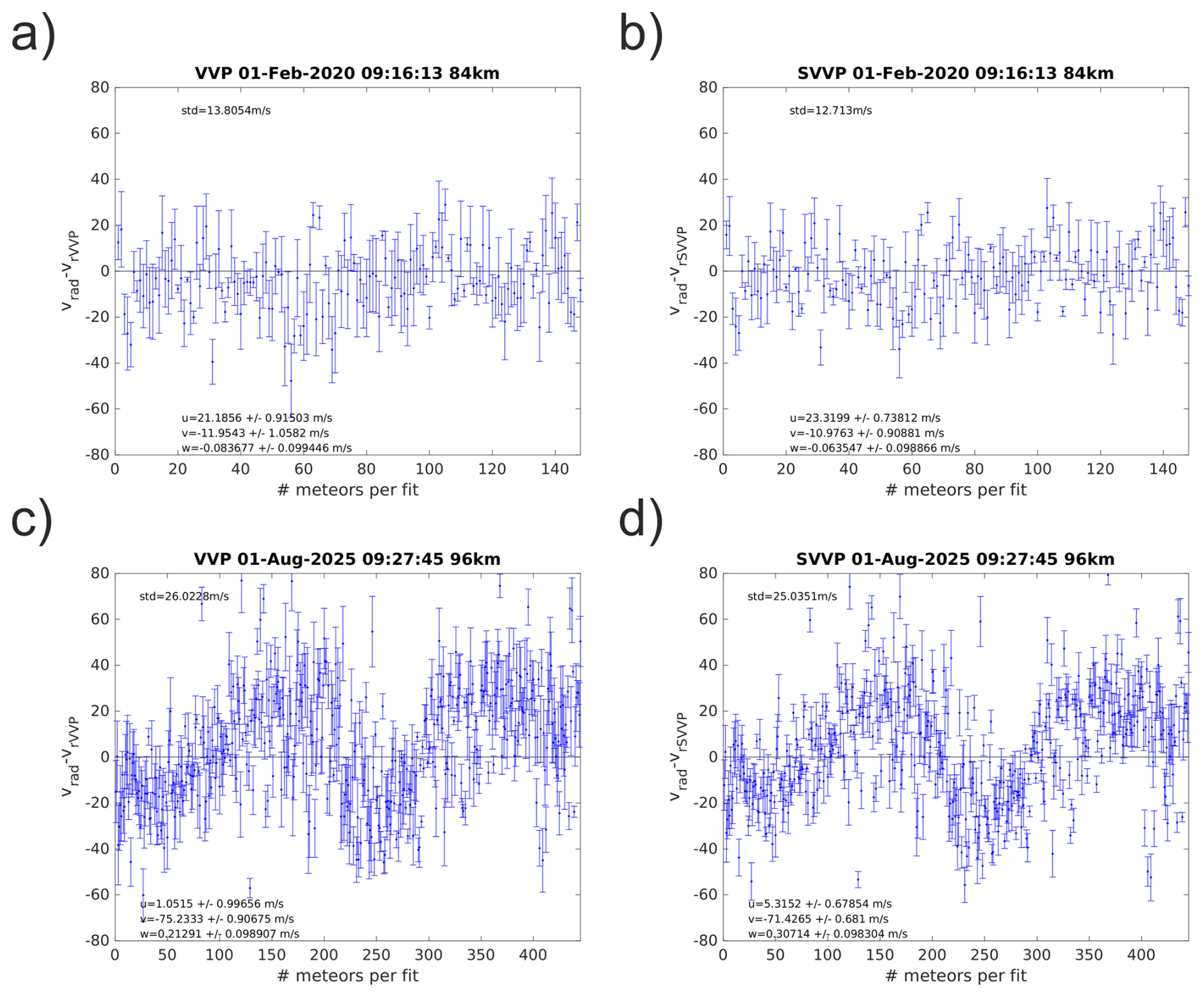
Figure 5 Fitting residuals for planar and spherical geometries for individual fits. The x-axis shows the number of meteor detections for this time-altitude bin. This is equivalent to time, but does not represent constant time steps. Panels (a, b) compare planar and spherical geometry for a typical scenario. Panels (c, d) highlight a case where the first-order approximation fails, and the residuals indicate an almost sinusoidal oscillation around the zero line.

This example is taken from the 60 min time resolution analysis and outlines the issue with two long temporal averages. The residuals indicate a sinusoidal oscillation likely related to a gravity wave moving through the domain. Again, the statistical uncertainties of the mean wind components for the SVVP are smaller compared to the planar implementation. The standard deviation from the zero line is more of an indication that more advanced retrievals could further reduce the scattering around the zero line. The fitting is implemented using an SVD solver (Press et al., 1992) (Fortran 77, adapted to MATLAB). The operational retrieval version does not store the SVD decomposition for each fit. Although the residuals indicate that there are cases where the first-order approximation starts to be no longer appropriate, it is expected that seasonal and climatological means hold. In particular, the 15 and 30 min temporal resolution data appear to be less affected compared to the 60 min temporal resolution. This also partially explains the scaling behaviour of the vertical winds with temporal resolution and spatial domain size, resulting in only partial sampling of wave periods or spatial scales.

However, to underline the robustness of the SVD, we present the normalized singular values for a single day in Fig. 6 to estimate also the condition number.

Figure 6 Singular values for one day and all fits, shown as a grey-shaded area and mean values (black dots).

The condition number is given by the largest and smallest singular values. For single precision, the recommended truncation to avoid numerical noise affecting the fitting results is $\mathrm{1}\times {\mathrm{10}}^{-\mathrm{5}}$ (Press et al., 1992). However, we have implemented the algorithm in double precision on an HPC. The singular values indicate that there is no rank deficiency for all fits that pass our quality control. The black dots represent mean values, and the grey shaded area visualizes the spread for all fits during one day.

The main benefit of the SVVP implementation is the error propagation, which permits estimating statistical uncertainties for all quantities. Both horizontal wind components show a peak of the Poisson distribution below 1 m s⁻¹ and a width of less than 5 m s⁻¹ in the tail. These statistical uncertainties are much smaller than the values obtained from monostatic all-sky fits with a similar retrieval setup. Monostatic analysis results in statistical uncertainties of 2–14 m s⁻¹. Only the vertical winds require some additional considerations for the error analysis. The algorithm uses a Tikhonov regularization, which mathematically acts similarly to a Bayesian retrieval for quantities with very low measurement response. The Doppler vertical winds show such a low measurement response, often at the lower and upper altitudes of the meteor layer; thus, the solution is dominated by the Tikhonov regularization (implicit apriori).

Figure 7 shows normalized histograms of the statistical uncertainties for the zonal, meridional, and vertical winds (without regularization). The effect of the Tikhonov regularization is basically given by the Lagrange multiplier ($\mathit{\alpha }=\mathrm{1}\times {\mathrm{10}}^{-\mathrm{2}}$), which acts as an inverse covariance (a priori covariance) (Rodgers, 2000). The covariances for the gradient terms reflect a Poisson distribution similar to the zonal and meridional winds. The statistical uncertainties for all fitted gradients show similar peak values and width of the error distributions, indicating that all quantities are rather well-constrained by the network and distribution of the meteor detections inside the field of view.

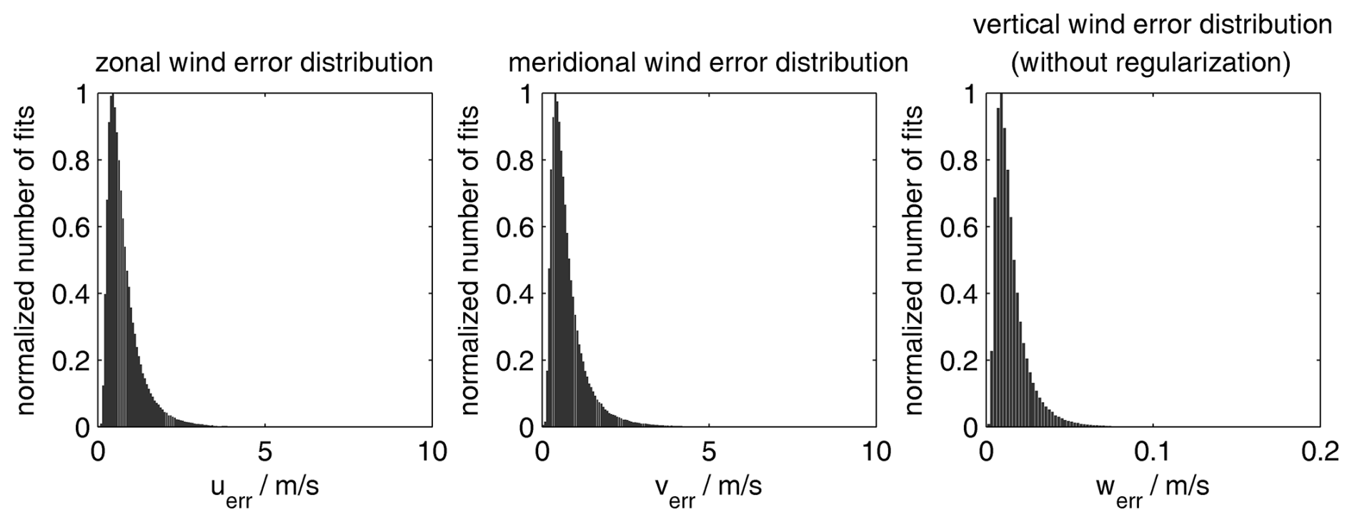
Figure 7 SVVP analysis covariances for the zonal, meridional, and vertical winds obtained from the retrieval for the instantaneous fits.

Figure 8 Same as Fig. 7, but for the gradient terms.

The covariance for the gradient terms also provides a benchmark for how the SVVP or VVP can be used to reconstruct the spatially resolved wind field (Zeng et al., 2024, 2026). The statistical uncertainty for the wind field increases with increasing distance from the reference point. This can be used as a threshold criterion for the largest accepted error for a given volume. Furthermore, the covariance permits extrapolating the statistical uncertainties for specific locations for dedicated comparisons such as Lidars, which often have a much smaller field of view (Ban et al., 2026; Qiao et al., 2025).

5 Results

In this section, we first present the seasonal and monthly mean wind variations and higher-order kinematic fields in the MLT region, based on the VVP plane geometry, spherical geometry (SVVP), their corresponding differences, and the 3DVAR+DIV method. We compare the SVVP and VVP model wind retrievals with the JAWARA and SE-WACCM-X datasets. We established a common data analysis pipeline to harmonize and reduce the data, removing the geophysical variability with periods shorter than a month. Mean winds, tides, and gravity waves are removed using the adaptive spectral filter (Baumgarten et al., 2018; Stober et al., 2020). We compute 31 d average zonal, meridional, and vertical daily mean winds with a boxcar for each altitude. All algorithms leverage identical nonlinear error propagation and data curation to avoid impacts on the results due to data gaps or other data filtering. The comparisons solely show the impact of the different geometries and spatiotemporal filters (circle of influence). The seasonal comparisons are based on a 31 d window with periodic boundary conditions. A similar procedure was applied in a previous study (Stober et al., 2021b). The median is computed when 40 % of all possible measurements for a time-altitude bin are available, but a reliable monthly mean is only obtained with a data coverage of 80 % or not more than 11 missing days per month. This threshold is considered the minimum required by the World Meteorological Organisation (WMO) for climatologies. All comparisons are conducted based on a 30 min temporal resolution, with a radius of 250 km for the SVVP, as a baseline. The radius of 250 km for the SVVP appeared to provide the best overlap between all four MR without including large blank spaces in the domain (see Fig. 2).

5.1 Climatologies of Mean Winds Derived from SVVP Retrieval

First, we compare the climatological mean state of the zonal, meridional, and vertical wind components based on the newly implemented SVVP algorithm (spherical geometry) with the previous VVP method (plane geometry). Figures 9 and C1 (see Appendix C) show the seasonal wind climatology of all three wind components in the MLT in both spherical (left column) and plane geometry (center column) with their corresponding differences (right column).

Figure 9 Monthly mean Zonal, meridional, and vertical wind components retrieved using the Volume Velocity Processing (VVP), showing the spherical geometry, plane geometry, and their corresponding differences.

The zonal (east–west) and meridional (north–south) wind components capture the horizontal circulation pattern. Zonal winds reflect the expected seasonal behaviour with eastward winds during hemispheric winter and the characteristic summer wind reversal from westward to eastward winds around 90 km. Furthermore, the zonal wind climatology captures the spring transition (March–April) at all altitudes into westward winds during the summertime, indicating a seasonal reversal of circulation. The opposite pattern is observed during the summer months; then, at the end of summer (late September–October), the wind shear weakens, leading to eastward winds at all altitudes. The difference plot indicates a systematic underestimate of the mean winds with altitude when using the plane geometry analysis relative to the spherical geometry. The difference in the eastward summer jet is up to 5 m s⁻¹ at 100 km altitude. The smallest differences between the two algorithms are found below 85 km altitude. Meridional winds also show the expected seasonal pattern with weak northward winds during winter and southward winds during the hemispheric summer. The largest differences between spherical and plane geometry are again observed at the upper altitudes of the meteor layer above 95 km, reaching almost 3 m s⁻¹. The vertical component exhibits a characteristic seasonal structure with upward and downward motions associated with large-scale atmospheric dynamics. The differences between spherical and plane geometry are in the order of 8 cm s⁻¹. Although the absolute difference appears to be small, it is considerable. Implementing the spherical geometry results in vertical wind magnitudes of about 6–8 cm s⁻¹ at around 90 km altitude, corresponding to the height of the zonal wind reversal and the maximum of the meridional wind.

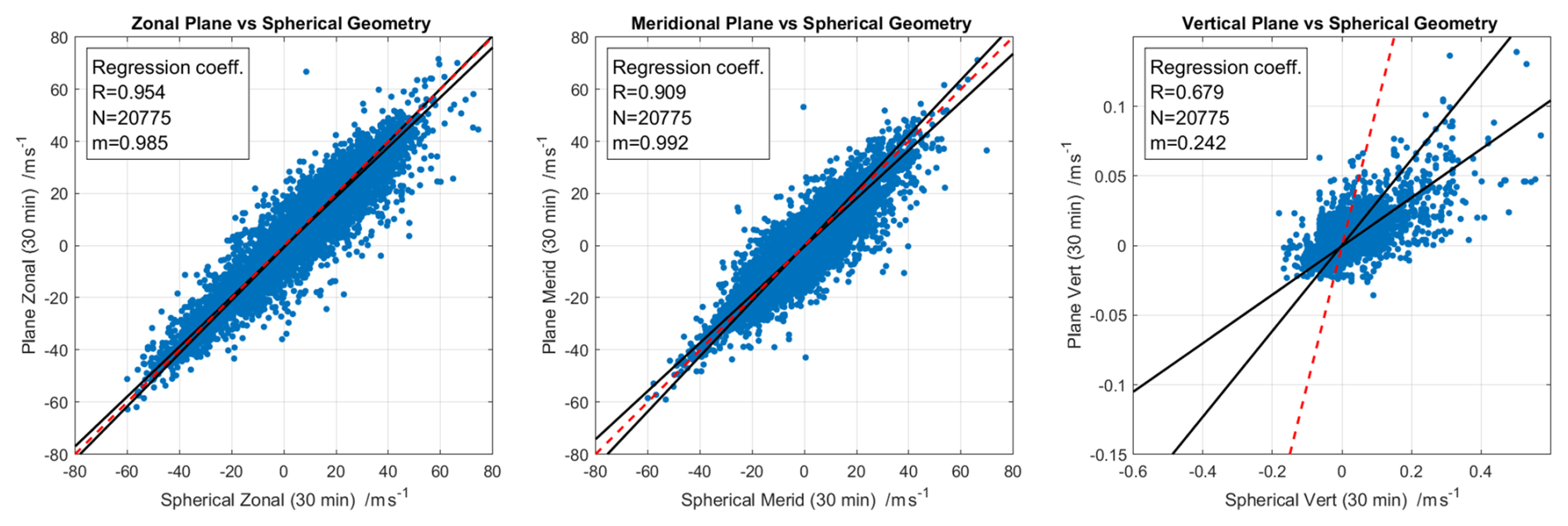
Figure 10 Correlation between the spherical geometry and plane geometry retrieved zonal, meridional, and vertical wind components using Volume Velocity Processing (VVP), based on the dataset used for Figs. 9 and C1. Each panel presents daily mean scatter points, robust regression fits, 1:1 reference lines, and annotated statistics (correlation coefficient (R), sample size (N), and the slope (m)). Regression lines are estimated using the iteratively reweighted least squares (IRLS) method with a bisquare (Tukey) weight function.

The comparison between the spherical and plane geometries in Volume Velocity Processing (VVP) retrievals shows a strong agreement for the horizontal wind components. However, the agreement is less good for the vertical wind component. Both zonal and meridional winds exhibit a high correlation coefficient of R=0.954 and R=0.909, respectively, with robust regression slopes exceeding 0.98–0.99, which indicates that there is no substantial bias between the algorithms for these wind components. This indicates that the geometry has only a minimal but still some impact on the large-scale flow estimates. In contrast, the vertical wind component shows a moderate correlation with a correlation coefficient of R=0.679 and a robust regression slope of 0.242, which reflects its great sensitivity to the geometrical assumptions and measurement uncertainties.

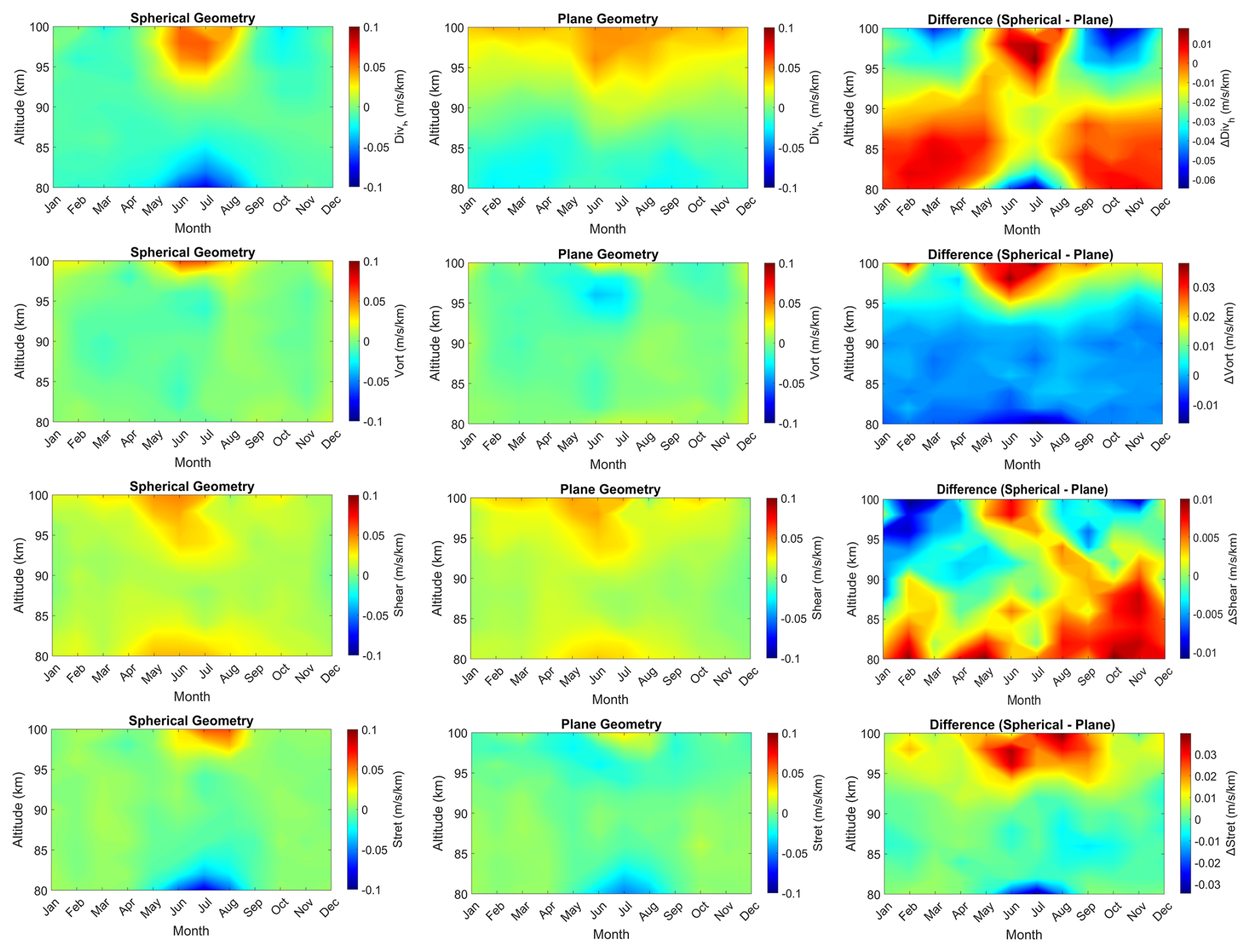
Figure 11 Monthly composites of horizontal divergence, shearing deformation, stretching deformation, and relative vorticity computed using Volume Velocity Processing (VVP), showing the spherical geometry and plane geometry with corresponding differences.

Figures 11 and C2 (see Appendix C) show the higher-order kinematic variables which are the horizontal divergence $\left(\frac{\partial u}{\partial x}+\frac{\partial v}{\partial y}\right)$, shearing deformation $\left(\frac{\partial v}{\partial x}+\frac{\partial u}{\partial y}\right)$, stretching deformation $\left(\frac{\partial u}{\partial x}-\frac{\partial v}{\partial y}\right)$, and the relative vorticity $\left(\frac{\partial v}{\partial x}-\frac{\partial u}{\partial y}\right)$, all within the magnitude of $\pm \mathrm{0.1}\mathrm{m}{\mathrm{s}}^{-\mathrm{1}}{\mathrm{km}}^{-\mathrm{1}}$ in both spherical and plane geometries along with their corresponding differences. These variables characterize different types of atmospheric horizontal motions, capturing divergence, eastward/westward (zonal) stretching, southwest/northeast stretching, and counter-clockwise rotation, represented as the positive values in the panels.

The seasonal and annual variations are exhibited in both geometric panels, but are more pronounced in the spherical geometry than in the planar geometry, as highlighted by the difference plots. Horizontal divergence is positive throughout the year at altitudes above 90 km during the mid-year (summer), pronouncedly seen in the spherical geometry, and the difference panel shows a big difference at higher altitudes above 96 km. There are positive differences at lower altitudes during winter and negative differences during summer, just up to 94 km. Stretching deformation exhibits similar characteristics to divergence, with higher values during summer.

Spherical geometric approximation shows a high impact on the shearing deformation and relative vorticity variables, revealing strong biases at higher altitudes with differences exceeding $\pm \mathrm{0.02}\mathrm{m}{\mathrm{s}}^{-\mathrm{1}}{\mathrm{km}}^{-\mathrm{1}}$ during summer months. The plane geometry approximation is seen to reproduce the large-scale characteristics of the atmospheric horizontal motions, and the spherical geometry approximation introduces significant changes and corrections, indicating the impact of Earth's curvature effects in the amplification of seasonal and altitudinal variability. The difference in the seasonal pattern of the horizontal divergence between VVP and SVVP is remarkable and indicates that it is important to account for the spherical representation of volumetric quantities. In plane geometry, the horizontal divergence below 86 km indicates a divergent situation throughout the year, while the opposite behavior is found above 96 km. This is counterintuitive, as this would imply a nearly constant upward vertical wind with only marginal seasonal modulation.

Figure 12 presents an intercomparison correlation of daily mean zonal, meridional, and vertical wind components computed using three temporal resolutions (15, 30, and 60 min) under spherical geometry. The objective of this analysis is to evaluate the consistency of the calculated winds across varying temporal resolutions equivalent to differing measurement statistics. Corresponding analyses for the plane geometry are provided in the supplementary material. The zonal winds (left panels) exhibit a nearly perfect linear relationship across all temporal correlation comparisons, with correlation coefficients exceeding 0.96 and regression slopes almost unity (m=0.99 and 1.027 for 15–30 min and 60–30 min, respectively). The meridional wind component (middle panels) also shows a strong correlation, though slightly weaker than the zonal wind, with a correlation coefficient close to 0.91 and regression slopes remaining close to 1 (m=0.976 and 1.062 for 15–30 min and 60–30 min, respectively), indicating only minor differences between the different temporal resolution datasets. These results suggest that the zonal wind flow is well resolved, and the moderate decrease in correlation in the meridional component reflects greater small-scale variability, typically in the geophysical flows due to mesoscale and synoptic-scale fluctuations.

Figure 12 Correlation comparing daily mean wind velocity components (zonal, meridional, and vertical) calculated for different temporal resolutions under spherical geometry. The top row compares 15 and 30 min temporal resolutions, while the bottom row compares 60 and 30 min temporal resolutions. Each panel shows the daily mean scatter point, robust regression fit (black solid line), 1:1 reference line (red dashed), and statistics indicating correlation coefficient (R), number of samples (N), and regression slope (m).

In contrast, the vertical wind component (right panels) shows correlation coefficients (R≈0.90), with regression slopes markedly deviating from unity, m=1.965 and 0.530 for 15–30 min and 60–30 min, respectively. This pronounced sensitivity to temporal resolution reflects the inherent transient nature of vertical velocities, which have very small magnitudes on seasonal scales. Vertical winds appear to be strongly influenced by small-scale gravity waves and their wave-mean flow interactions, driven by wave breaking. It is observed that shorter temporal resolutions preserve more high-frequency variability and, thus, capture more of the high-frequency gravity wave spectrum, minimizing effects due to incomplete sampling of spatiotemporal gravity wave variability (Qiao et al., 2025).

On the other hand, a higher temporal resolution suffers from data sparsity and might systematically underestimate the vertical winds. This comparison demonstrates that while horizontal wind components (zonal and meridional) are highly consistent across temporal resolutions, the vertical wind exhibits a strong dependence on geometry and temporal scale. This is further underlined by the residual analysis shown above for the 60 min analysis, which clearly indicated the effects of transient gravity waves inside the domain.

Figure 13 presents an intercomparison of the higher-order kinematic variables, including horizontal divergence, shearing deformation, stretching deformation, and relative vorticity components derived under spherical geometry for three temporal resolutions (15, 30, and 60 min). As in the previous analysis of the wind components, the 30 min temporal resolution is used as the reference to evaluate the influence of temporal scale on these kinematic variables. Corresponding analyses for the plane geometry are provided in the Supplementary material.

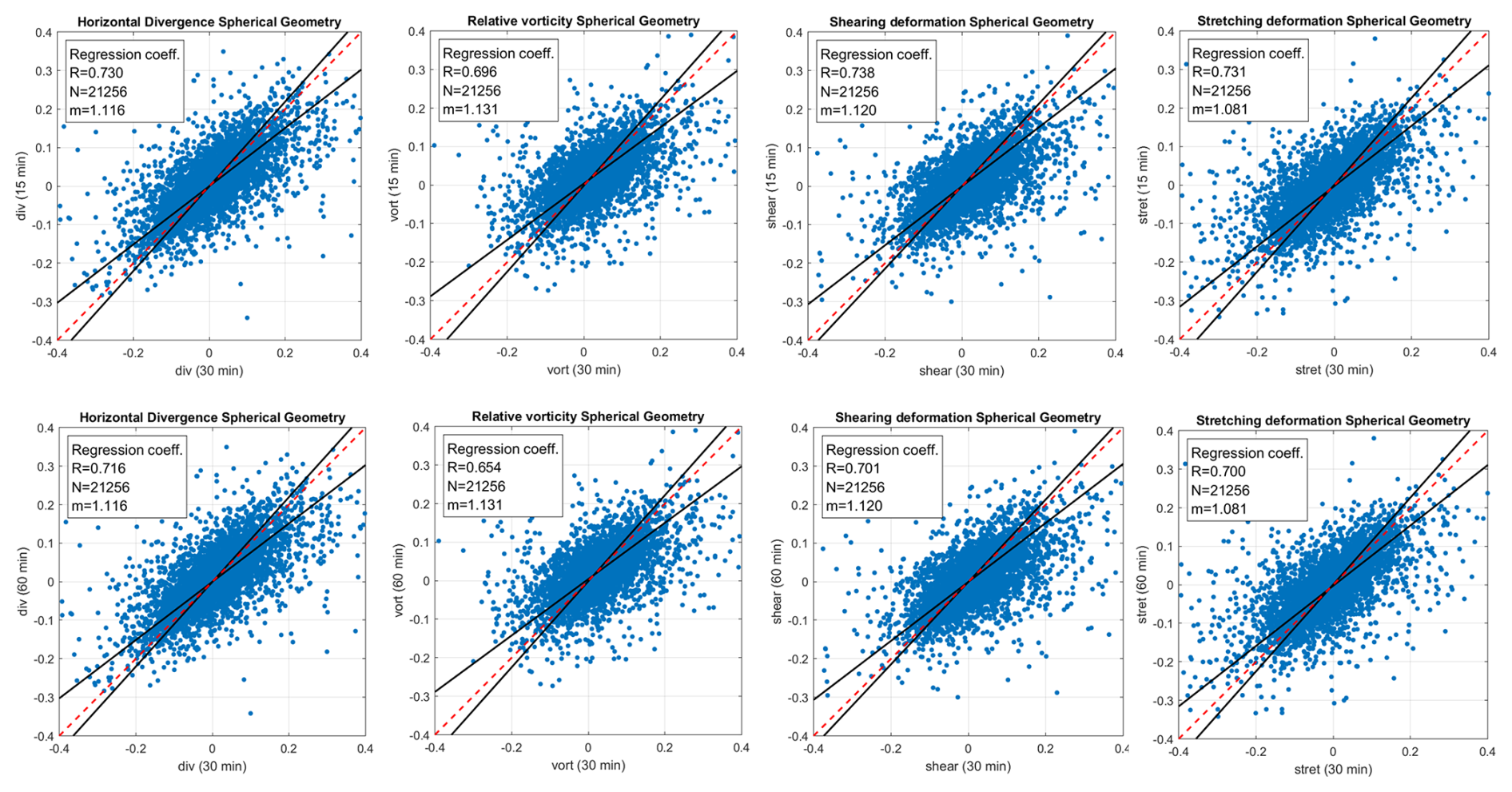
Figure 13 Comparison of correlations of high-order kinematic variables: horizontal divergence, shearing deformation, stretching deformation, and relative vorticity computed for different temporal resolutions under spherical geometry. The top row compares 15 and 30 min temporal resolutions, while the bottom row compares 60 and 30 min temporal resolutions. Each panel shows the daily mean scatter point, robust regression fit (black solid line), 1:1 reference line (red dashed), and statistics indicating correlation coefficient (R), number of samples (N), and regression slope (m).

Table 2 Correlation coefficients and regression slopes of horizontal winds (u,v), vertical wind (w), and higher-order kinematic variables (divergence, vorticity, shear, and stretching deformation) retrieved from the full dataset (January 2021–June 2026) at 30 min intervals, compared against 15 and 60 min resolutions.

The correlation between the datasets is moderate, with a correlation coefficient ranging from approximately 0.68–0.78. Shearing deformation shows the highest correlation, with a correlation coefficient of R≈0.76 for the 15–30 min and R≈0.71 for the 60–30 min comparison, while relative vorticity exhibits a slightly lower correlation coefficient of R≈0.75 for the 15–30 min and R≈0.68 for the 60–30 min comparison. Robust regression slopes for all variables remain close to unity ($m\approx \mathrm{1.08}-\mathrm{1.11}$), reflecting general linear agreement but with noticeable scatter.

Although the derived kinematic variables maintain reasonable consistency across all temporal resolutions, they exhibit more variability than the wind components (see Figs. 11 and C2). This highlights that temporal resolution significantly influences diagnostics of the kinematic variables, particularly of the horizontal divergence and relative vorticity, which are indicators for wave breaking and flow stability (Vadas et al., 2003; Vadas, 2013).

We also performed an initial comparison of the vertical winds derived from the VVP and SVVP with the state-of-the-art reanalysis JAWARA (Sato et al., 2025; Koshin et al., 2022, 2025) and the free-running SE-WACCM-X model (Liu et al., 2024). SE-WACCM-X has indicated a substantially improved vertical transport for NO_x at polar latitudes compared to coarse-resolution WACCM-X runs (Liu, 2025). JAWARA and SE-WACCM-X vertical winds have been reduced following the procedure outlined in Stober et al. (2021b). We used the reference coordinate and a circle of radius 300 km to compute an average for all grid points that fell into that volume to match the observational characteristics of the NMRC.

Figure 14 presents the estimated seasonal cycle of mean vertical velocity averaged over the 80–90 km altitude layer for JAWARA and SE-WACCM-X (in both panels), and the 80–90 km (left panel) and 84–94 km (right panel) altitude layers for VVP and SVVP. We selected these two altitude windows to match the observational summer-season vertical-velocity peak in VVP/SVVP (84–94 km) and the vertical velocity peak in SE-WACCM-X (80–90 km). JAWARA exhibits a less pronounced vertical structure of the vertical velocities with altitude. This comparison allows for an assessment of the variability in SVVP and VVP. All models reproduce a broadly consistent annual cycle with near-zero or negative values in winter, a pronounced upward maximum around June-August, and a return to near-zero or negative values by autumn. This agreement across all four independent approaches supports the physical characteristics of the summer upwelling signal in the mesosphere–lower thermosphere at these altitudes. The peak amplitudes of the vertical velocities for the 80–90 km altitude layer are 0.8, 3.4, 2.1, and 3.8 cm s⁻¹ for VVP, SE-WACCM-X, JAWARA, and SVVP, respectively, whereas for the 84–94 km altitude layer, the peak amplitudes are 1.2 cm s⁻¹, and 5.9 cm s⁻¹ for VVP and SVVP respectively. In both altitude ranges, VVP shows the weakest summer maximum. SVVP and SE-WACCM-X have the highest and most similar peak amplitudes, especially in the 80–90 km range compared to the 84–94 km layer. JAWARA shows more negative values in winter and autumn than the meteor radar retrievals and SE-WACCM-X, and its summer peak is lower than those of SVVP and SE-WACCM-X but higher than that of VVP.

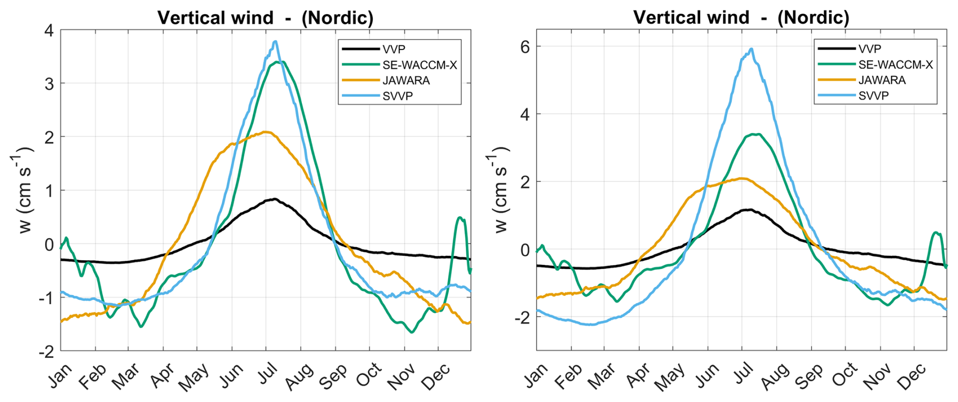
Figure 14 Vertical winds from the JAWARA reanalysis and the free-running SE-WACCM-X model averaged over the altitudes 80–90 km (both panels), with VVP and SVVP analysis averaged over 80–90 km (left panel) and 84–94 km (right panel).

Furthermore, the above-shown comparison is, in the first place, a physical consistency check rather than an absolute validation. There are still idealizations in the data analysis, such as the assumption of incompressibility in 3DVAR+DIV or other divergence-based vertical winds, as well as the assumption that a first-order approximation provides a reasonable description of the higher-order flow field inside the measurement domain. Currently, we speculate that the differences in vertical wind magnitudes in JAWARA are likely related to the much coarser spatial resolution of about 2° in longitude and latitude, essentially removing gravity waves. SE-WACCM-X is a free-running model and not yet tuned to match observational fields, and some physical processes are still parameterized, which can lead to changes in the absolute magnitude of the vertical velocity.

5.2 Climatologies of Mean Winds from 3DVAR+DIV Retrievals

The 3DVAR+DIV retrieval is dedicated to resolving small-scale gravity waves within a domain using an advanced ill-posed tomographic inversion. The main advantage of the algorithm is that it applies to arbitrary wind fields and only includes a mathematical smoothness constraint to address the ill-posed mathematical problem. The 3DVAR+DIV adds the continuity equation to provide one additional condition, resulting in more reliable vertical winds. However, the retrieval intrinsically uses the incompressibility condition and a simplified boundary condition (zero mean vertical wind over the entire column of each grid cell) for the vertical integration of the divergence-derived vertical wind. However, our choice of the boundary condition results essentially in the removal of all seasonal features in the vertical winds due to the larger errors for the retrieved quantities. Another important issue is that the bias correction is applied on smaller spatial domains and much shorter time scales compared to the SVVP, resulting in a larger uncertainty of the debiasing overlaying any seasonal pattern.

The seasonal wind climatology of all three wind components derived with the 3DVAR+DIV retrieval is illustrated in Fig. 15. The horizontal winds show a consistent climatological pattern and interannual variability, as well as for the vertical winds (despite a magnitude scaling issue).

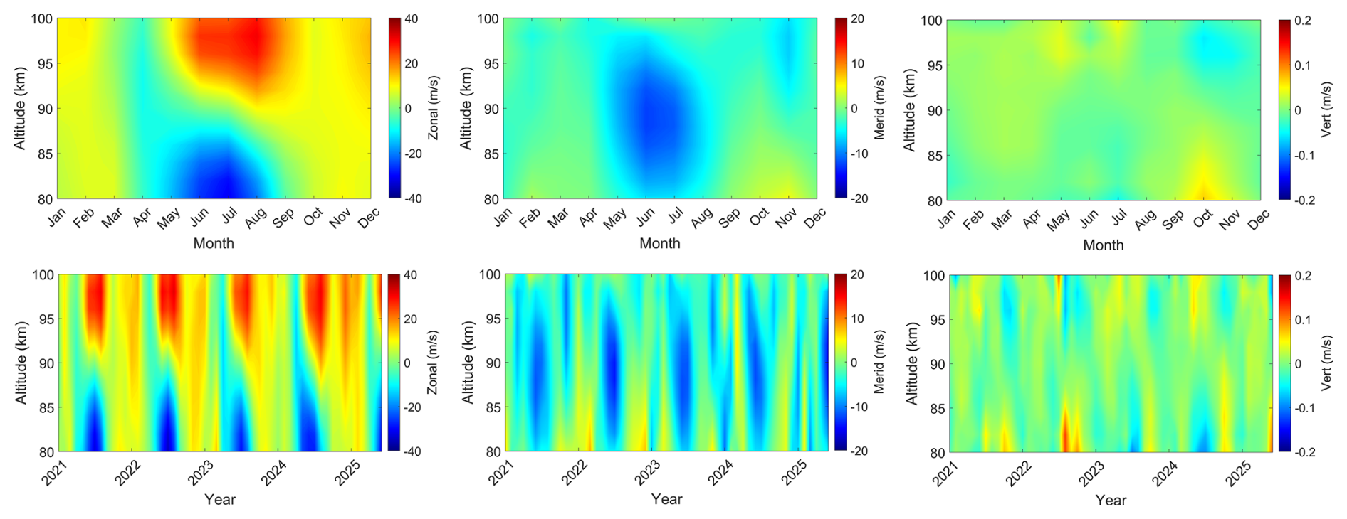
Figure 15 Monthly and seasonal composites of zonal, meridional, and vertical wind components utilizing 3DVAR+DIV.

This magnitude offset is attributed to the spatial derivatives and projection errors inside each grid cell (not yet implemented in spherical geometry), the much lower measurement statistics per grid cell, and Tikhonov regularization in the 3DVAR+DIV retrieval framework. The vertical component exhibits upwelling in late winter across all altitudes, with a particularly enhanced region between approximately 85 and 95 km. Another upwelling is observed between 95 and 100 km as summer approaches. During summer, a broad region is dominated by downwelling between approximately 83 and 93 km altitude. In autumn, a second, more intense downwelling region is shown at higher altitudes (95–99 km), persisting into early winter before gradually weakening.

However, considering the overall benefits of the 3DVAR+DIV to capture the small-scale features that remain unresolved in the SVVP, the very good agreement of the horizontal wind seasonal pattern outlines the performance of the retrieval. The current version of the 3DVAR+DIV algorithm debiases the vertical winds for each grid cell instantaneously, thereby largely removing seasonal variability. Comparing the regularization strength for different 3DVAR+DIV retrievals revealed that the remaining seasonal variability changed by only 25 % with respect to the seasonal amplitudes. The regularization strength is a unitless parameter that deflates or inflates the a priori covariances of the L2 regularization. The default a priori covariance for the horizontal winds is ${\mathit{\sigma }}_{u,v}=\mathrm{30}\mathrm{m}{\mathrm{s}}^{-\mathrm{1}}$ and ${\mathit{\sigma }}_w=\mathrm{5}\mathrm{m}{\mathrm{s}}^{-\mathrm{1}}$ for the vertical wind component. However, instantaneous winds start deviating for individual grid cells depending on the measurement statistics. A regularization strength of α=0.4 (corresponds to a 1.5 times larger default error covariance) still reliably reproduces the horizontal winds, but produces more spurious outliers in the vertical winds. We define an outlier as 4σ of the total variance of all data during the 5 years. These outliers start to disappear at a regularization strength of α=0.8. A regularization strength of α=150 (corresponds to only 1$/$6th of the default error covariance) removes most of the small-scale variability and only sustains the seasonal pattern.

5.3 Sensitivity 3DVAR+DIV Wind Retrievals to Tikhonov regularization

Figure 16 illustrates the sensitivity of 3DVAR+DIV wind retrievals to the Tikhonov regularization parameter controlling the mathematical coupling between grid cells describing the smoothness of the retrieved wind field α (α=0.4 and α=150), compared with the SVVP retrieval method. The dates were selected arbitrarily and correspond to times with good data quality (Geminid meteor shower in December) and moderate/normal data quality (January) concerning the number of detections. A small Tikhonov parameter provides more freedom to the solver to obtain small-scale variability, whereas an increased Tikhonov parameter enforces smoothness, suppressing small-scale features.

All retrievals show a dominant large-scale southwesterly wind flow pattern, consistent with the prevailing synoptic forcing during the analyzed period. However, noticeable deviations in the wind magnitude and spatial smoothness are evident among the retrievals. The 3DVAR+DIV retrieval method with a small Tikhonov regularisation constraint (α=0.4; left panel) weakens the background smoothness constraint, allowing the solution to capture finer-scale flow features, likely related to small-scale gravity waves forced by tropospheric weather patterns, orography, or secondary wave generation in the stratosphere due to the breaking of primary GW (Vadas et al., 2024; Becker et al., 2022; Becker and Vadas, 2020). This approach enhances the depiction of local circulation but also introduces small-scale noise and spatial inconsistencies, reflecting the stronger influence of the divergence constraint and reduced smoothing. In contrast, increasing the Tikhonov parameter to α=150 (middle panel) strengthens the constraint, suppressing local fluctuations and producing a more coherent flow field with smoother gradients at the expense of hampering the retrieval of smaller-scale fluctuations in the wind field. The SVVP retrieval (right panel) yields the smoothest and most conservative wind field among the three approaches, with minimal spatial variability due to its approximation of only first-order inhomogeneities within the radar sampling volume.

Quantitatively, the mean horizontal wind components reveal variations among the methods. In the first case (1 January 2021), the zonal and meridional wind components for 3DVAR+DIV with α=0.4 are approximately $-\mathrm{18.4}\pm \mathrm{1.8}\mathrm{m}{\mathrm{s}}^{-\mathrm{1}}$ and $-\mathrm{47.8}\pm \mathrm{1.8}\mathrm{m}{\mathrm{s}}^{-\mathrm{1}}$ respectively, while increasing α to 150, yields smoother, more stable wind slow of $-\mathrm{18.7}\pm \mathrm{0.1}\mathrm{m}{\mathrm{s}}^{-\mathrm{1}}$ and $-\mathrm{34.2}\pm \mathrm{0.1}\mathrm{m}{\mathrm{s}}^{-\mathrm{1}}$ with significantly reduced uncertainties and due to the stronger regularization stabilizing inversion showing smoother spatial gradients. The second case (14 December 2024) benefits from more data. For 3DVAR+DIV with α=0.4, the zonal and meridional wind components are approximately $\mathrm{49.2}\pm \mathrm{1.6}\mathrm{m}{\mathrm{s}}^{-\mathrm{1}}$ and $-\mathrm{71.3}\pm \mathrm{1.5}\mathrm{m}{\mathrm{s}}^{-\mathrm{1}}$, respectively. Increasing α to 150 yields smoother and more stable wind speeds of $\mathrm{54.6}\pm \mathrm{0.1}\mathrm{m}{\mathrm{s}}^{-\mathrm{1}}$ (zonal) and $-\mathrm{51.5}\pm \mathrm{0.1}\mathrm{m}{\mathrm{s}}^{-\mathrm{1}}$ (meridional), again showing significantly reduced uncertainties due to the enhanced regularisation and resulting smoother spatial gradients. The low α case exhibits greater deviations in regions with sparse radar coverage, leading to localized wind direction and magnitude biases. The SVVP method produces horizontal mean winds of roughly $-\mathrm{29.5}\pm \mathrm{2.8}\mathrm{m}{\mathrm{s}}^{-\mathrm{1}}$ and $-\mathrm{41.9}\pm \mathrm{2.5}\mathrm{m}{\mathrm{s}}^{-\mathrm{1}}$, and for the second case $\mathrm{53.1}\pm \mathrm{2.2}\mathrm{m}{\mathrm{s}}^{-\mathrm{1}}$ and $-\mathrm{65.4}\pm \mathrm{1.7}\mathrm{m}{\mathrm{s}}^{-\mathrm{1}}$, characterized by relatively larger uncertainties and weaker wind magnitudes due to its limited ability to resolve horizontal gradients and its susceptibility to the propagation of measurement noise through the least-squares fitting.

These findings underscore a fundamental trade-off between spatial resolution and retrieval stability. Reduced regularization strength enhances the variability of the resultant retrieved wind field, permitting the investigation of the gravity wave forcing of the MLT due to orography, weather patterns, or polar vortex-induced primary or secondary gravity waves (Vadas et al., 2024), critical for understanding wind flow dynamics in the MLT, but increases susceptibility to noise due to the sparsity of data. Conversely, higher regularization yields smoother, dynamically consistent solutions suitable for data assimilation and climatological applications describing a large-scale mean flow. The 3DVAR+DIV effectively resolves spatial heterogeneity while maintaining physical coherence when the regularization parameter is carefully optimized, a capability not obtained with the SVVP approach. Currently, the 3DVAR+DIV performs best with regularization strengths between $\mathit{\alpha }=\mathrm{0.4}-\mathrm{5}$. These values for the Tikhonov regularization were derived based on the Hunga-Tonga gravity wave that was detected in the wind measurements above the NMRC and CONDOR (Stober et al., 2023) and validated against the gravity wave resolving High Altitude Mechanistic Circulation Model (HIAMCM) (Vadas et al., 2023a, b; Stober et al., 2024).

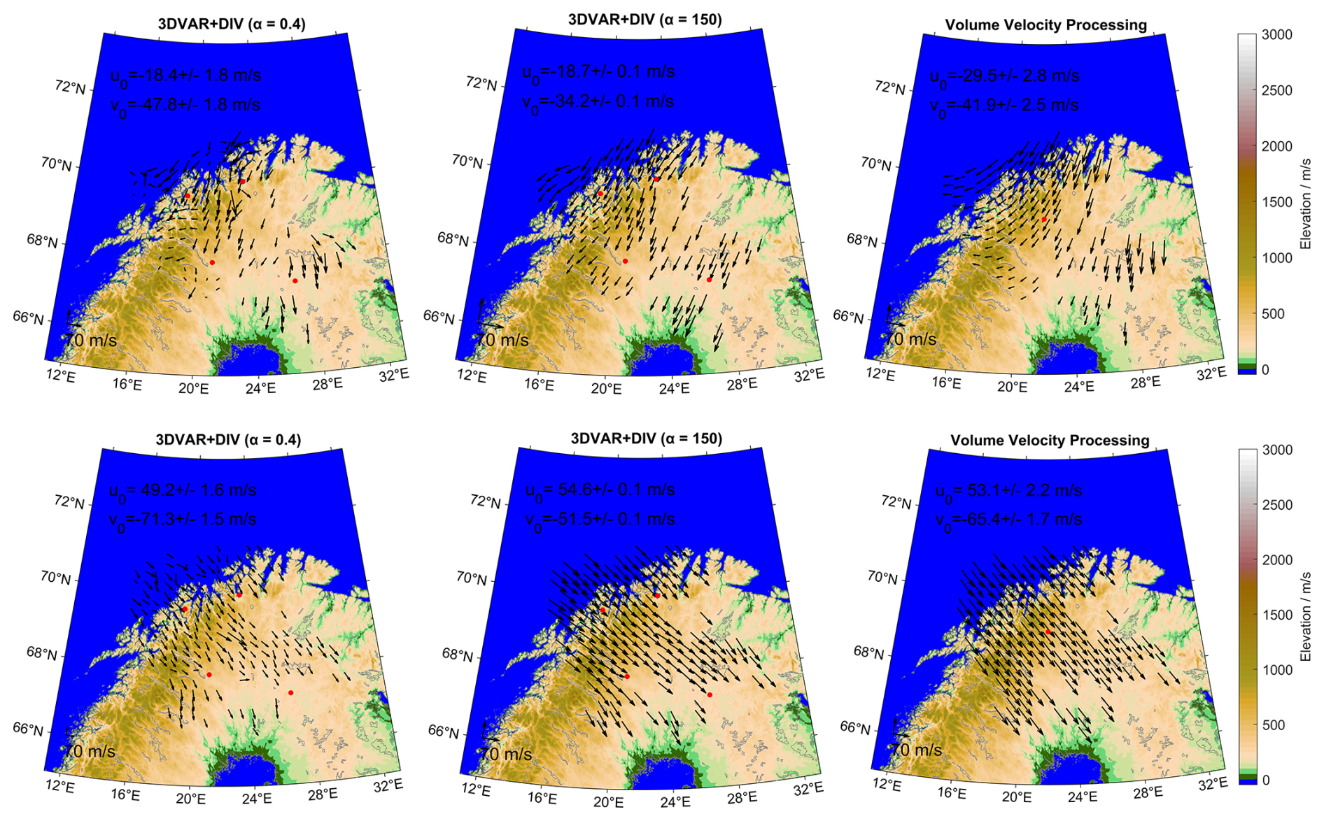
Figure 16 Horizontal wind fields over the NORDIC Meteor Radar Cluster for 00:00 UTC on 1 January 2021 (top row) and on 14 December 2024 (bottom row). The wind field is derived using 3DVAR+DIV with Tikhonov regularization parameters of 0.4 (left panel), 150 (middle panel), and SVVP (right panel). The background shows the topography (m a.s.l.), while black arrows represent horizontal wind vectors. Red dots are the station locations for 3DVAR+DIV and the reference location for SVVP. The colorbar shows elevation in meters above sea level.

Figure 17 presents the correlation between SVVP and 3DVAR+DIV wind retrievals with regularization parameters of 0.4 and 150. This analysis further quantifies the relationship between the two retrieval methods. In the comparison between VVP in spherical geometry and 3DVAR+DIV with a regularization parameter of 0.4, both zonal and meridional wind components are highly correlated, with correlation coefficients of R=0.894 and R=0.845, respectively, and corresponding robust regression slopes are 0.934 (zonal) and 0.946 (meridional).

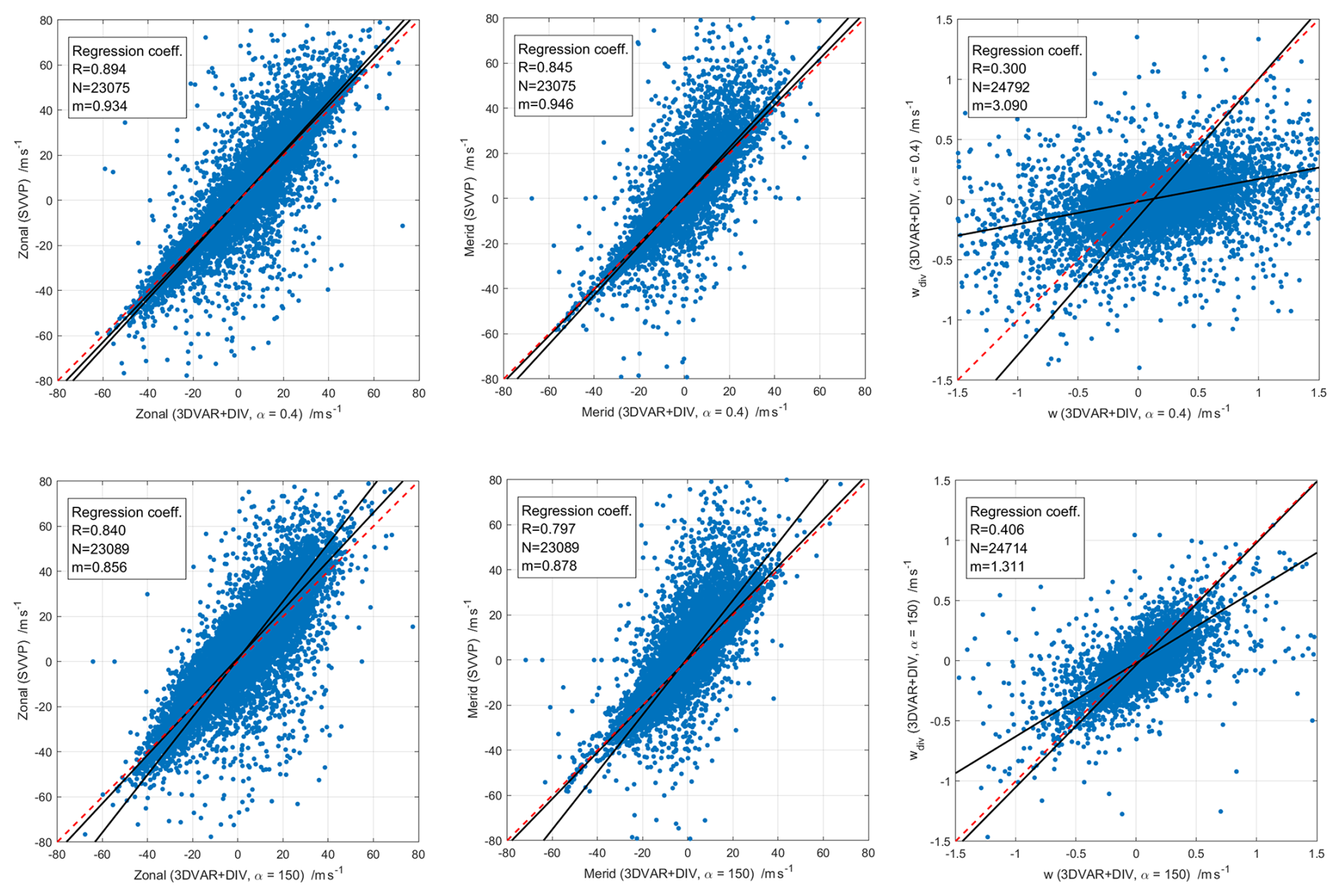
Figure 17 Correlation between Volume Velocity Processing (VVP) and 3DVAR+DIV retrieved zonal, meridional, and vertical wind components. Each panel includes daily mean scatter points, robust regression fits, 1:1 reference lines, and annotated statistics (correlation coefficient (R), sample size (N), and the slope (m)).

In the comparison between VVP in spherical geometry and 3DVAR+DIV with a regularization parameter of 150, both zonal and meridional wind components are highly correlated, with correlation coefficients of R=0.840 and R=0.797, respectively, and corresponding robust regression slopes are 0.856 (zonal) and 0.878 (meridional). These results indicate that both algorithms exhibit no substantial bias in representing mean horizontal winds. Additionally, the third and sixth panels assess the internal consistency of the 3DVAR+DIV retrievals by comparing the vertical wind derived from the retrieved horizontal divergence field (w_div) with the Doppler vertical wind (w), for regularization parameters of 0.4 and 150, respectively. At a regularization parameter of 0.4, the correlation is low (R=0.300) with a regression slope of 3.090, suggesting that w_div exhibits substantially larger amplitude than w and weakly tracks its spatial and temporal variations. At a regularization parameter of 150, the agreement improves, with the correlation coefficient increasing to R=0.406 and the regression slope decreasing to 1.311, closer to unity. This indicates that stronger regularization of the horizontal divergence field brings w_div into closer amplitude agreement with w.

6 Discussion

Multistatic meteor radar networks are increasingly being established worldwide. These networks also cover much larger domain areas and have rather different layouts, considering the combination of passive and active radars. The Nordic Meteor Radar Cluster is unique in that it only includes monostatic radars with good overlap in the network (Stober et al., 2021a, 2022), although passive receiver stations can be added in the future. Multistatic networks also offer the possibility to implement different mathematical approaches to infer 3D winds, such as the Bayesian 3DAVR+DIV retrieval (Stober et al., 2022; Qiao et al., 2025) or algebraic least-square fits based on different implementations of the VVP (Waldteufel and Corbin, 1979; Stober and Chau, 2015; Chau et al., 2017; Zeng et al., 2024).

The 3DVAR+DIV retrieval solves the ill-posed and ill-conditioned tomographic problem for a pre-defined geographic domain. The main advantage of the method is the retrieval of arbitrary wind fields and small-scale features or non-linearities in the wind field. Considering the entropy definition introduced by Shannon (1948) and Shannon and Weaver (1963), we calculate the Shannon measurement response, an additional diagnostic to estimate the mixing of a priori information and contributions from the measurements on the final solution of the state vector (see Fig. 18).

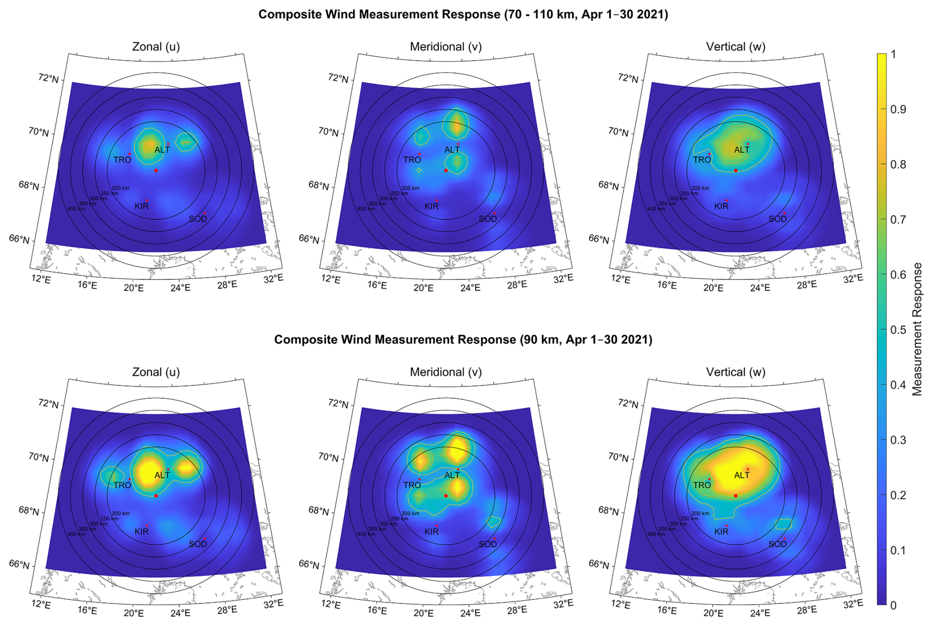
Figure 18 Composite wind measurement response for the zonal, meridional, and vertical wind components from 1–30 April 2021 at 70–110 km (top row) and 90 km (bottom row) altitude, retrieved using the 3DVAR+DIV method. Red dots indicate station locations, with their labels identifying each station; the unlabeled dot marks the central reference point used for the SVVP retrievals. The concentric rings represent distance in km from this central reference point.

In this study, we used the measurement response as a proxy to determine the most reliable circle of influence for the SVVP. This diagnostic also reveals correlations inside the domain volume due to the implemented mathematical smoothness constraint. These correlations are estimated by averaging kernels, a standard diagnostic in many remote sensing applications (Sica and Haefele, 2015; Hagen et al., 2018; Krochin et al., 2022, 2024). An increased measurement response is important to ensure that each fitted parameter can be estimated from the observations. This is, in particular, worth considering for mathematically ill-conditioned problems. Due to the random occurrence of meteors inside the measurement domain, there might be situations where not all three wind components can be determined with the same precision and accuracy. Typically, ill-conditioned parameters appear to be inflated. The VVP and SVVP are based on least-squares fits and approximate the spatial variability by expanding the wind field into a Taylor series. The coefficients are solved by an algebraic solution to a linear set of equations. The advantage of the VVP/SVVP is the reduced computational resources compared to a 3DVAR+DIV retrieval. In this study, we present a novel implementation of the VVP in spherical coordinates (SVVP) and approximate the ellipsoidal shape of the Earth for iso-surfaces based on WGS84 coordinates (Zeng et al., 2024). There have been previous implementation attempts of the VVP in spherical coordinates by mixing Cartesian and spherical coordinates (Chau et al., 2017). However, our resulting equations differ substantially in the gradient terms. A comparison of the VVP in plane geometry and the newly developed SVVP shows remarkable differences in the higher-order kinematic terms, such as horizontal divergence, relative vorticity, and stretching and shearing deformation. The horizontal wind components exhibit smaller but still noticeable deviations. In particular, the horizontal divergence shows a characteristic altitude variation in plane geometry with positive values above 90 km during the entire year.

Such a vertical structure also leads to biases in vertical winds derived from horizontal divergence, resulting in climatological vertical wind speeds of several m s⁻¹, which seem physically unrealistic for a seasonal value (Chau et al., 2017). The implemented SVVP shows a clear seasonal pattern and no systematic altitude structure for the horizontal divergence, which also results in much more realistic seasonal vertical winds in the order of several cm s⁻¹. The SVVP algorithm performs best on seasonal time scales when the underlying assumptions are statistically valid. However, on short time-scales, the algorithm might not capture non-linear gradients induced by certain gravity waves or bores (Smith et al., 2017). Furthermore, the gradient terms and mean winds are physically only meaningful for the selected reference point.

The vertical winds calculated in this study were debiased following information theory (Rodgers, 2000). The most robust estimate of the vertical motion over longer periods is provided by the meteor ablation altitude and reaches values of a few hundred meteors per decade (Stober et al., 2012a, 2014; Dawkins et al., 2023b). Therefore, it is reasonable to subtract this mean vertical wind from the climatology and the long-time series to remove potential offsets in the network due to the alignment of the antennas or possible phase offsets in the interferometry. These bias corrections are almost constant with altitude and in the order of 1–8 cm s⁻¹ for diameters of 200 and 250 km in the SVVP analysis. Larger domains tend to produce also larger and altitude-dependent bias corrections.

We also performed a sensitivity study, defining circles of influence around the selected reference coordinates of 200–400 km in radius with a step size of 50 km. Furthermore, we analyzed all the measurements collected by the Nordic Meteor Radar Cluster from 2021–2024 using temporal resolutions of 15, 30, and 60 min to determine the impact of temporal averaging. For the comparison, we selected a temporal resolution of 30 min as a reference. The temporal resolution had almost no influence on the derived horizontal wind components and resulted in a correlation of 0.96 for the zonal and 0.91 for the meridional wind.

However, the vertical wind shows clear scaling behavior, with larger values at the lower temporal resolution and smaller values in the 15 min analysis. Spectral analysis of horizontal and vertical winds (see Fig. 19) shows that all retrievals indicate a $-\mathrm{5}/\mathrm{3}$ slope for the gravity wave range.

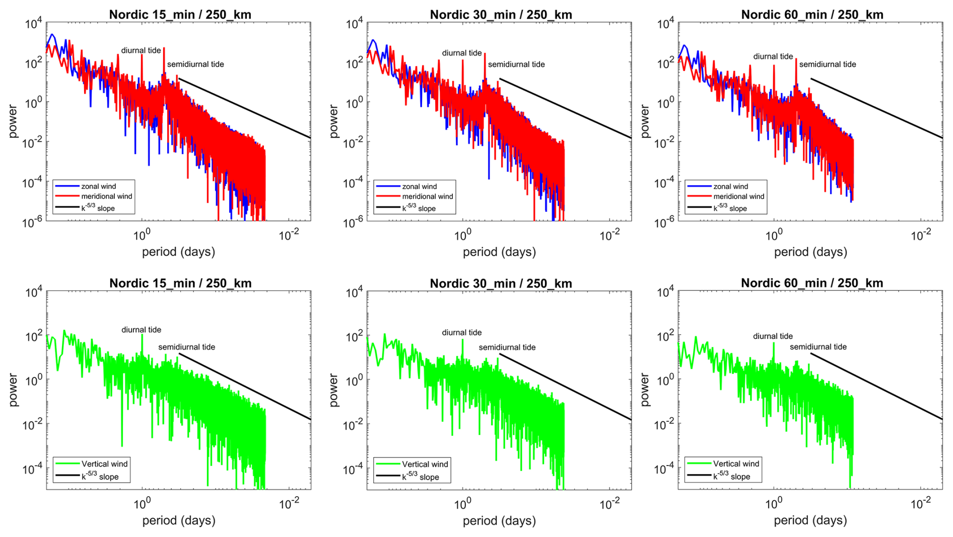
Figure 19 Temporal spectra of zonal and meridional winds at 90 km altitude for 15, 30, and 60 min, respectively. Spectra are computed with SVVP data spanning 1 July 2024–31 December 2024.

Furthermore, lidar observations from McMurdo have shown that the largest vertical velocities occur at the smallest scales (Chu et al., 2026). However, due to the sparser sampling, these larger vertical velocities start to be undersampled at the 15 min temporal resolution. This is, in particular, the case during times with fewer meteor detections (afternoon time in UTC), which results in an underestimation of the retrieved vertical winds. The horizontal mean winds are less affected and indicate only a rather small effect (see Fig. 7). A temporal resolution of 60 min already suffers from smearing effects. Fast small-scale gravity waves (ducted gravity waves) have substantial phase speeds (Snively et al., 2007; Snively and Pasko, 2008; Stober et al., 2013) and can propagate up to 150–200 km within one hour through the domain, resulting in sampling issues that inflate the observed vertical winds (opposite effect to the 15 min retrieval). Currently, the 30 min temporal resolution appears to be the most robust retrieval considering sufficient sampling and temporal resolution.

Comparing different circles of influence for the Nordic Meteor Radar Cluster reveals the best consistency for radii of 200 and 250 km, with a tendency towards systematic deviations at increasing radii. In particular, the horizontal divergence, and consequently the vertical wind, appears to be inflated for larger circles of influence compared to the smaller domains with 200–250 km radius. Only the 200–250 km circle is truly multistatic; when we increase the volume even more, not all wind components are equally well determined in all parts of the domain. This becomes clearer when looking at the measurement response from the 3DVAR+DIV shown in Figs. 2 18, and 20.

Figure 20 Composite meteor number per grid point from 1–30 April 2021 at 70–110 km (left) and 90 km (right) altitude, retrieved using the 3DVAR+DIV method. Red dots indicate station locations, with their labels identifying each station; the unlabeled dot marks the central reference point used for the SVVP retrievals. The concentric rings represent distance in km from this central reference point.

Only the 200 and 250 km circles of influence exhibit an almost homogeneous spatial distribution in the measurement response, whereas the 400 km circle indicates areas with dark blue color or lies even outside the pre-defined 3DVAR+DIV domain. Furthermore, when the domain size is increased too much, additional projection errors due to the elliptical shape of the Earth become significant, which are not yet accounted for in the derived equations but are crucial for determining reliable vertical winds. Vertical winds are also more sensitive to the overall statistics inside the domain; therefore, the upper and lower edges of the meteor layer are problematic due to the lower number of meteor detections, and thus the vertical winds are only trustworthy between 85–95 km altitude.

Another important aspect of the SVVP and also the 3DVAR+DIV algorithm is their applicability to other meteorological networks, such as weather radars or multistatic Lidar wind measurements in the boundary layer. Both algorithms require information about the range, time, angle of arrival, and line-of-sight velocity. The domains can be fairly flexible, adapted to specific needs. However, both algorithms can get computationally expensive when applied to very large data sets or very high-resolution domains, e.g., a weather radar network with a domain grid of 1–2 km spatial resolution and a few hundred meters vertical spacing between layers. However, it could be beneficial to resolve small-scale updrafts in thunderstorms or other small-scale dynamics that are often hidden or unresolved in standard data analysis.

7 Conclusions

Accurate estimation of three-dimensional wind fields in the mesosphere and lower thermosphere (MLT) is crucial for advancing our understanding of atmospheric dynamics and variability. However, it has posed a longstanding significant challenge in atmospheric science, particularly regarding the reliable retrieval of vertical wind. The MLT region is influenced by radiative forcing from both above (space) and wave-driven dynamics from the middle atmosphere, posing challenges for GCMs to reproduce a realistic mean state of the dynamics (Stober et al., 2021b; Hindley et al., 2022). Neutral winds in the MLT play a vital role in mediating the transport of energy and momentum, thereby coupling the upper and lower atmosphere and shaping the global circulation patterns.

In this paper, we present 3D spatially resolved wind fields in the MLT using advanced retrieval techniques. Specifically, we introduce a novel SVVP method in spherical coordinates to improve the physical consistency of wind retrievals, and we compare its performance against the conventional VVP method in plane geometry and the 3DVAR+DIV method. Utilizing meteor radar observations spanning from 2021 to summer 2025 from the Nordic Meteor Radar Cluster, we analysed data statistics, seasonal mean wind characteristics, and inter-method correlations. Wind retrievals were performed with temporal resolutions of 15, 30, and 60 min and radii ranging from 200–400 km in steps of 50 km. The 30 min temporal resolution was used as the reference to evaluate the impact of temporal averaging. All retrieval methods reproduced the expected climatological pattern of mean winds; however, correlation analyses revealed some discrepancies among methods. The 3DVAR+DIV approach better captures small-scale variability and is more suitable for arbitrary wind fields, whereas the VVP/SVVP methods produce a smoother wind field and are computationally less expensive. Notable differences emerged in the wind components and the higher-order kinematic variables between the plane and the spherical implementations of the VVP. The horizontal wind components showed smaller but still systematic deviations. In particular, the horizontal divergence in the plane geometry indicated a characteristic altitude variation with positive bias throughout the year, pointing to systematic issues. The SVVP exhibited a clearer seasonal pattern and no systematic altitude structure, which also resulted in more self-consistent seasonal variations in vertical winds in the order of several cm s⁻¹, which falls within the range of theoretical expectations from SE-WACCM-X (grid size comparable to the 3DVAR+DIV retrievals) and JAWARA. Our findings highlight the importance of a correct geometric representation of the implemented retrieval and temporal averaging to ensure sufficient statistics to obtain reliable MLT winds. The newly improved SVVP method demonstrates enhanced physical consistency, although an absolute validation requires alternate observations to verify the obtained results. It provides a robust framework for future investigations of MLT dynamics, including wave-mean flow interactions and momentum coupling processes in the middle/upper atmosphere for longer time series. In contrast, the 3DVAR+DIV retrieval is beneficial for high-resolution case studies.

Appendix A: Latitude implementation Spherical coordinates

We also calculated the SVVP equations using latitude θ, instead of a colatitude. Please note that θ here denotes the latitude. We used both sets of equations to remove ambiguities in the signs for each term.

$$\begin{array}{}\text{(A1)}& \begin{array}{rl}u& =r\cos \mathrm{\Phi }\dot{\mathit{\varphi }}\\ v& =r\dot{\mathit{\theta }}\\ w& =\dot{r}\end{array}\end{array}$$

The gradient terms take the form;

$$\begin{array}{}\text{(A2)}& {\displaystyle \frac{\partial u}{\partial x}}\cdot e_x& {\displaystyle }={\displaystyle \frac{\partial \dot{\mathit{\varphi }}}{\partial \mathit{\varphi }}}\cdot e_{\mathit{\varphi }}\text{(A3)}& {\displaystyle \frac{\partial u}{\partial y}}\cdot e_y& {\displaystyle }=(-\mathrm{2}\dot{\mathit{\varphi }}\cdot \sin \mathit{\theta }+\cos \mathit{\theta }\cdot {\displaystyle \frac{\partial \dot{\mathit{\varphi }}}{\partial \mathit{\theta }}})\cdot e_{\mathit{\theta }}\text{(A4)}& {\displaystyle \frac{\partial v}{\partial x}}\cdot e_x& {\displaystyle }={\displaystyle \frac{\mathrm{1}}{\cos \mathit{\theta }}}{\displaystyle \frac{\partial \dot{\mathit{\theta }}}{\partial \mathit{\varphi }}}\cdot e_{\mathit{\varphi }}\text{(A5)}& {\displaystyle \frac{\partial v}{\partial y}}\cdot e_y& {\displaystyle }=({\displaystyle \frac{\partial \dot{\mathit{\theta }}}{\partial \mathit{\theta }}}-\dot{\mathit{\theta }}\cdot \tan \mathit{\theta })\cdot e_{\mathit{\theta }}\end{array}$$

The reconstructed wind field components take the form;

$$\begin{array}{}\text{(A6)}& \begin{array}{rl}u(\mathit{\lambda },\mathrm{\Phi })=& u_{\mathrm{0}}({\mathit{\lambda }}_{\mathrm{0}},{\mathrm{\Phi }}_{\mathrm{0}})+{\displaystyle \frac{\partial \dot{\mathit{\varphi }}}{\partial \mathit{\varphi }}}{r}_{\mathrm{m}}\cos {\mathit{\theta }}_{\mathrm{m}}\mathrm{\Delta }\mathit{\varphi }\\ & +\cos {\mathit{\theta }}_{\mathrm{0}}\cdot {\displaystyle \frac{\partial \dot{\mathit{\varphi }}}{\partial \mathit{\theta }}}{r}_{\mathrm{m}}\mathrm{\Delta }\mathit{\theta }-\mathrm{2}{u}_{\mathrm{0}}\cdot {\displaystyle \frac{\sin {\mathit{\theta }}_{\mathrm{0}}}{r_{\mathrm{0}}\cos {\mathit{\theta }}_{\mathrm{0}}}}{r}_{\mathrm{m}}\mathrm{\Delta }\mathit{\theta }\\ v(\mathit{\lambda },\mathrm{\Phi })=& v_{\mathrm{0}}({\mathit{\lambda }}_{\mathrm{0}},{\mathrm{\Phi }}_{\mathrm{0}})+{\displaystyle \frac{\mathrm{1}}{\cos {\mathit{\theta }}_{\mathrm{0}}}}{\displaystyle \frac{\partial \dot{\mathit{\theta }}}{\partial \mathit{\varphi }}}{r}_{\mathrm{m}}\cos {\mathit{\theta }}_{\mathrm{m}}\mathrm{\Delta }\mathit{\varphi }\\ & +{\displaystyle \frac{\partial \dot{\mathit{\theta }}}{\partial \mathit{\theta }}}{r}_{\mathrm{m}}\mathrm{\Delta }\mathit{\theta }-v_{\mathrm{0}}\cdot {\displaystyle \frac{\tan {\mathit{\theta }}_{\mathrm{0}}}{r_{\mathrm{0}}}}{r}_{\mathrm{m}}\mathrm{\Delta }\mathit{\theta }\\ w(\mathit{\lambda },\mathrm{\Phi })& =w_{\mathrm{0}}({\mathit{\lambda }}_{\mathrm{0}},{\mathrm{\Phi }}_{\mathrm{0}}).\end{array}\end{array}$$

Appendix B: Non-linear error propagation

All retrievals use a nonlinear error propagation as weighting of the least-squares solver, which is implemented as the singular-value decomposition (SVD). The line-of-sight velocity uncertainty is provided in the mpd- or met-file data from the commercial software package of each radar. The angular uncertainty of 2° for each angle is included by performing a Gaussian error propagation. We calculate all statistical uncertainties based on the radial velocity equation;

$$\begin{array}{}\text{(B1)}& {\displaystyle }& {\displaystyle }\begin{array}{rl}{\displaystyle }{v}_{\mathrm{r}}\left({\mathit{\varphi }}_{\text{err}}\right)& {\displaystyle }=\left|{\displaystyle \frac{\mathrm{d}{v}_{\mathrm{r}}}{\mathrm{d}\mathit{\varphi }}}\right|\cdot \mathrm{\Delta }\mathit{\varphi }\\ {\displaystyle }& {\displaystyle }=|-u\cdot \sin \mathit{\varphi }\sin \mathit{\theta }+v\cdot \cos \mathit{\varphi }\sin \mathit{\theta }|\cdot \mathrm{\Delta }\mathit{\varphi }\end{array}\text{(B2)}& {\displaystyle }& {\displaystyle }\begin{array}{rl}{\displaystyle }& {\displaystyle }{v}_{\mathrm{r}}\left({\mathit{\theta }}_{\text{err}}\right)=\left|{\displaystyle \frac{\mathrm{d}{v}_{\mathrm{r}}}{\mathrm{d}\mathit{\theta }}}\right|\cdot \mathrm{\Delta }\mathit{\theta }\\ {\displaystyle }& {\displaystyle }=|u\cdot \cos \mathit{\varphi }\cos \mathit{\theta }+v\cdot \sin \mathit{\varphi }\cos \mathit{\theta }-w\cdot \sin \mathit{\theta }|\cdot \mathrm{\Delta }\mathit{\theta }.\end{array}\end{array}$$

There is also a contribution of the mean winds in the error propagation, which is estimated from the radial wind equation as follows;

$$\begin{array}{}\text{(B3)}& {\displaystyle }{v}_{\mathrm{r}}\left(u_{\text{err}}\right)& {\displaystyle }=\left|{\displaystyle \frac{\mathrm{d}{v}_{\mathrm{r}}}{\mathrm{d}u}}\right|\cdot \mathrm{\Delta }u=\left|\cos \mathit{\varphi }\sin \mathit{\theta }\right|\cdot \mathrm{\Delta }u\text{(B4)}& {\displaystyle }{v}_{\mathrm{r}}\left(v_{\text{err}}\right)& {\displaystyle }=\left|{\displaystyle \frac{\mathrm{d}{v}_{\mathrm{r}}}{\mathrm{d}v}}\right|\cdot \mathrm{\Delta }v=\left|\sin \mathit{\varphi }\sin \mathit{\theta }\right|\cdot \mathrm{\Delta }v\text{(B5)}& {\displaystyle }{v}_{\mathrm{r}}\left(w_{\text{err}}\right)& {\displaystyle }=\left|{\displaystyle \frac{\mathrm{d}{v}_{\mathrm{r}}}{\mathrm{d}w}}\right|\cdot \mathrm{\Delta }w=\left|\cos \mathit{\theta }\right|\cdot \mathrm{\Delta }w\end{array}$$

The uncertainties in the winds are solved iteratively. The initial weight is zero during the first iteration. All successive iterations are performed by propagating the SVD fitting uncertainties.

Furthermore, we include a sampling error. We define an arbitrary reference time and altitude using a boxcar in altitude and time, with a height of 3 km and a time of 2 h. All meteors that are detected within this boxcar are weighted by a Gaussian weight depending on how far the meteor in altitude and time occurred relative to the reference of the grid cell center. The magnitude of this weighting function is calculated from the spatio-temporal Laplace filter, which estimates a predictor using the altitudes above and below, as well as the time steps before and after a reference altitude-time bin. A more detailed description can be found in Stober et al. (2018); Gudadze et al. (2019); Hindley et al. (2022).

Appendix C: Wind Seasonal Climatology

Here we present an analysis of the time series using the 31 d boxcar average for all data used (2021 to summer 2025) for wind components derived from SVVP and VVP. Figures C1 and C2 present the seasonal climatologies of the zonal, meridional, and vertical wind components and the higher-order kinematic variables, respectively, derived in the SVVP and VVP. Figure C1 presents the zonal, meridional, and vertical wind components, which exhibit the typical climatological behaviour and reveal some interannual variability. All differences between the two algorithms are also reproduced with similar magnitude over the entire time series. Most remarkable are the changes in the vertical wind magnitudes during hemispheric summer. Apparently, for the years 2021 and 2022, both algorithms obtained 30 % larger wind upwelling during summer than for the other years. This increased upwelling is accompanied by stronger eastward zonal winds during the summer, whereas the years with weaker vertical winds also indicate a slightly different transition from the winter circulation to the hemispheric summer wind pattern.

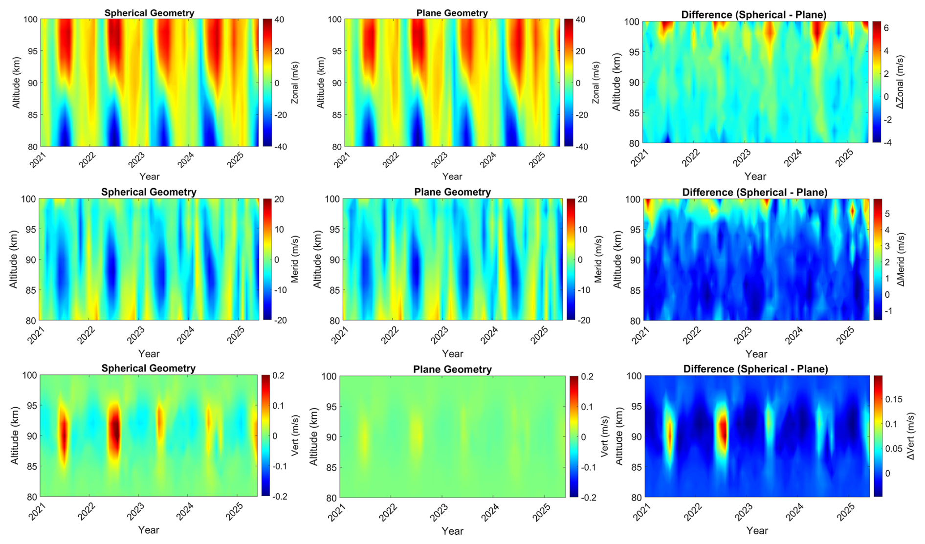
Figure C1 Seasonal mean zonal, meridional, and vertical wind components retrieved using the Volume Velocity Processing (VVP), showing the spherical geometry, plane geometry, and their corresponding differences.

Figure C2 Seasonal composites of horizontal divergence, shearing deformation, stretching deformation, and relative vorticity using Volume Velocity Processing (VVP), showing the spherical geometry and plane geometry with corresponding difference.