A multimodal approach to derive cloud microphysics in deep convective clouds from polarized measurements of the cloudbow

We present a new method to derive droplet size distributions in clouds consisting of multiple modes using aircraft based polarized measurements of the cloudbow. The retrieval builds onto the existing single mode parametric approach, but allows up to three modes in the droplet size distribution (DSD), where each mode is described by a gamma distribution of effective radius r_eff and effective variance v_eff. While the DSDs of shallow cumulus or stratiform clouds are often well described by single mode distributions, this does not hold in the presence of drizzle or rain and the measured polarized radiance is not accurately described by a single mode fit. We show that allowing multiple modes in those cases not only improves the fit significantly but also shows good agreement to the Rainbow Fourier Transform (RFT), which derives an arbitrary distribution. The parametric retrieval fits polarized phase functions derived by Mie theory to the measured polarized radiance, such that, for the retrieval of large droplets, new Mie calculations were performed to include effective radii up to 1000 µm. In a sensitivity analysis, the uncertainty in the retrieval of large effective radii is tested as the polarized phase functions become less distinct. For effective radii up to about 800 µm, the relative mean bias is found to be less than 10 %. The relative noise (standard deviation) increases from about 4 % for typical cloud droplets of 10 µm to about 30 % around 500 µm before decreasing again towards even larger effective radii. For the effective variance, increased uncertainties are found both for r_eff≲3 µm and r_eff≳200 µm. In between, the determination of the effective variance is also possible with an uncertainty of less than 50 %. With the found uncertainties in mind, the new multimode approach is applied to a case study of a deep convective cloud measured during the PERCUSION campaign in 2024 in the vicinity of Barbados, where a rainbow is observed in the RGB image of the camera and also the radar reflectivity shows clear signals of rain. While the single mode retrieval cannot accurately explain the measured signal close to the rainbow observation, the capability of the multimode retrieval to disentangle the signal is demonstrated qualitatively. Furthermore, the individual results from the multimode retrieval are evaluated against the droplet size distributions derived from the Rainbow Fourier Transform (RFT) and similarities are found in most cases, although the results from the RFT show instabilities with negative values in the DSD. Currently, the RFT is only capable to retrieve droplet size distributions with radii up to 100 µm, and hence is limited in regions with precipitating droplets. This is where the potential of the multimode approach comes into play as it is capable to detect modes of large effective radii up to 1000 µm, which does not only improve the result of a single mode retrieval, but might also allow to learn about physical processes such as rain initiation in deep convective clouds.

1 Introduction

Clouds occur in a large variety almost everywhere on the globe covering on average 67 % of the surface (King et al., 2013). Hence, they largely influence the Earth's energy budget, having both a warming and a cooling effect. The cooling effect is mainly due to the reflection of solar shortwave radiation back to space, which is determined by the optical properties of clouds, and thus their phase (liquid, ice or mixed-phase) and the size and shape of the cloud particles (e.g. Liou, 2002). Cloud optical properties can be investigated by observing the cloud particles in situ or by remote sensing techniques from ground, aircraft or space using either passive spectral or imaging techniques as well as active radar and lidar techniques. Classical passive satellite retrievals are based on a bispectral approach described by Nakajima and King (1990) to derive the cloud effective radius (r_eff,  Hansen and Travis, 1974) and the cloud optical thickness τ from reflectance measurements in an absorbing and a non-absorbing channel in the visible, near- or shortwave infrared range of the spectrum. While the effective radius is a measure for the effective size of the particles with the observed optical properties, there is no information about the width of the cloud droplet size distribution (CDSD) from the bispectral approach. However, when it comes to cloud microphysical processes, the width of the cloud droplet size distribution is thought to play a crucial role in the onset of precipitation with broader distributions being more favorable for the formation of larger drizzle and rain droplets (e.g.,  Brenguier and Chaumat, 2001; Chandrakar et al., 2016). From passive remote sensing, information about the cloud droplet size distribution is gained from measurements of the polarized radiance in the scattering angle range between 135° and 165°, the range of the cloud- and rainbow (e.g. Bréon and Goloub, 1998; Pörtge et al., 2023). In this region, the polarized phase function P₁₂ is highly sensitive to the cloud droplet size distribution, and under the assumption of a monomodal gamma distribution as defined by Hansen (1971), the effective radius r_eff and the effective variance v_eff of the observed cloud area are determined by comparing the measurements to precalculated phase function tables from Mie theory (Mie, 1908). The assumption of a single-mode gamma distribution is widely used (Deirmendjian, 1964; Hansen, 1971; Tampieri and Tomasi, 1976; Alexandrov et al., 2015) and also verified by in situ observations (e.g., Sect. 2.1.4 of Pruppacher and Klett, 2010; Miles et al., 2000).

The polarimetric retrieval has successfully been applied to both space- and airborne measurements, e.g. to measurements of the Polarization and Directionality of the Earth's Reflectances instrument (POLDER; Deschamps et al., 1994; Bréon and Goloub, 1998; Bréon and Doutriaux-Boucher, 2005; Shang et al., 2015), the Research Scanning Polarimeter (RSP; Cairns et al., 1999; Alexandrov et al., 2012a), the Airborne Hyper-Angular Rainbow Polarimeter (AirHARP; Martins et al., 2018; McBride et al., 2020) and the Airborne Multiangle SpectroPolarimetric Imager (AirMSPI ; Diner et al., 2013; Xu et al., 2018). With the launch of NASA's Plankton, Aerosol, Cloud, ocean Ecosystem (PACE) mission in 2024 (Werdell et al., 2026), new spaceborne polarimetric measurements from the Hyper-Angular Rainbow Polarimeter 2 (HARP2) are available, which can be used to derive cloud droplet size distributions (Smith et al., 2026).

Here, we use measurements from the polarization resolving RGB cameras of the airborne spectrometer of the Munich Aerosol Cloud Scanner (specMACS; Weber et al., 2024) to which Pörtge et al. (2023) applied the polarimetric retrieval. The instrument has been operated onboard the German High-Altitude and LOng range research aircraft (HALO;  Krautstrunk and Giez, 2012) during several recent field campaigns, such as the Elucidating the role of clouds-circulation coupling in climate (EUREC⁴A; Stevens et al., 2021) campaign, the HALO-(AC)³ campaign (Wendisch et al., 2024) and the Persistent EarthCARE underflight studies of the ITCZ and organized convection (PERCUSION; Groß et al., 2026) as part of the larger ORCESTRA campaign (Stevens et al., 2026). Originally, specMACS consisted of two hyperspectral line cameras that measure in the wavelength range between 400 and 2500 nm (Ewald et al., 2016). Prior to the EUREC⁴A campaign the instrument has been extended by two downward looking polarization resolving Phoenix 5.0 MP Polarization Model cameras (Pörtge et al., 2023). In 2024, two more sideward-facing polarization cameras were integrated, providing an overall field of view of about 91°×220° (along × across track) for the observation of deep convective clouds reaching flight altitudes during the PERCUSION campaign. Each camera covers a field of view of about 91°×78° and has a resolution of 2448 × 2048 pixels (along × across track,  Weber et al., 2024). Moreover, the cameras provide simultaneous measurements at a frame rate of 5−8 Hz resulting in a high temporal resolution. Together, this allows to aggregate the scattered polarization signal from cloud targets at a spatial resolution of about 100 m×100 m and an angular resolution of 0.3° (Pörtge et al., 2023).

Until now, the polarimetric retrieval from specMACS has mainly been applied to boundary layer clouds. During the EUREC⁴A campaign, the retrieval was used on non-precipitating shallow cumulus clouds (Pörtge et al., 2023; Pörtge, 2024) and Weber et al. (2026b, a) had a look on the cloud microphysics of arctic mixed-phase clouds observed in marine cold air outbreaks during the HALO-(AC)³ campaign. In those cases, where the assumption of a monomodal gamma distribution holds for the liquid cloud phase (Alexandrov et al., 2015), Volkmer et al. (2024b) performed an analysis of the retrieval uncertainties based on synthetic model simulations and found a mean bias ± standard deviation of $(-\mathrm{0.2}\pm \mathrm{1.30})$ µm for the retrieved effective radius. For the effective variance, an uncertainty of (0.02±0.05) was found.

However, the flights of the recent PERCUSION campaign targeted the Intertropical Convergence Zone (ITCZ), which is characterized by a trimodal distribution of cloud types, namely shallow cumulus, congestus and cumulonimbus (Johnson et al., 1999). During the first part of the campaign from 9 August–6 September 2024, HALO was based in Sal, Cape Verde in the eastern tropical Atlantic before being transferred to Barbados to target the western part of the tropical Atlantic basin from 6–30 September 2024. In both parts, all of the three kinds of tropical clouds defined by Johnson et al. (1999) were identified and next to the cloudbow, the much more intense rainbow could be observed in coexistence in particular on the lower cloud sides where precipitation falls out. In this case, the assumption of a single mode gamma distribution does not hold any longer. Even though the rainbow is in general much narrower and more intense than the cloudbow, the superposition of the two signals causes erroneous results in the single mode retrieval, usually in terms of an overestimation of the actual cloud effective radius.

One method, which does not require any a priori assumption on the shape of the CDSD, is the so-called Rainbow Fourier Transform (RFT; Alexandrov et al., 2012b). It is based on an integral transform that decomposes the observed signal into a sum of pre-calculated phase functions over size bins. Alexandrov et al. (2015) observed, that the resulting droplet size distribution (DSD) from the RFT is usually well described by a superposition of multiple single mode gamma distributions, such that they introduced a method to decompose the DSD into several modes, each defined by an effective radius and variance. However, one issue of the RFT is that the derived DSDs can show artifacts caused by the non-orthogonality of the polarized phase functions. This is corrected by an universal correction function independent of the actual size distribution (Alexandrov et al., 2012b). The RFT has further been developed on a database of equally spaced (0.5 µm) polarized phase functions from Mie theory integrated over a very narrow triangular size distribution of width 0.1 µm up to a maximum radius of 100 µm. Hence, the resulting size distributions n(r) fulfill the condition $n(r>\mathrm{100}\mathrm{\mu }\mathrm{m})=\mathrm{0}$ per definition, while actual rain droplets have sizes up to several millimeters (Pruppacher and Klett, 2010, Sect. 2.1.6). Therefore, using the RFT in cases where cloud and rain droplets coexist would require a huge database of polarized phase functions calculated from Mie theory, not only in terms of calculated radii but also in terms of the angular resolution (0.2° in the case of Alexandrov et al., 2012b), since the number of oscillations increases for larger radii. While the RFT remains formally valid in case of large radii, its practicability deteriorates for our applications.

To this end, we introduce a new multimodal fitting approach in this paper analogue to the polarimetric retrieval, but allowing the appearance of multiple (single-mode) gamma distributions. We start in Sect. 2 with the description of the retrieval algorithm and Sect. 3 shows an example on real measurements. Further, Sect. 3.1 includes a comparison of individually measured cloud targets to the existing RFT. Finally, Sect. 4 discusses the introduced method and reveals how this can be used to investigate scientific questions.

2 Retrieval description

This sections gives a detailed description of the presented multimodal cloud droplet size distribution retrieval. We start with the theoretical basis and the mathematical formulation of the problem, followed by the actual numerical implementation.

2.1 Theoretical framework

The scattering of electromagnetic waves on spherical particles is fully described by Mie theory (Mie, 1908). In general, for radiation traveling along the positive z-axis the scattered electric field vector ${\mathit{E}}_{\text{sc}}=(E_l,E_r{)}_{\text{sc}}^T$ is related to the incoming electric field vector ${\mathit{E}}_{\text{in}}=(E_l,E_r{)}_{\text{in}}^T$ by the scattering amplitude matrix (e.g., Bohren and Huffman, 1998, Sect. 3.2)

$$\begin{array}{}\text{(1)}& {\displaystyle }{\left(\begin{array}{c}{E}_l\\ E_r\end{array}\right)}_{\text{sc}}={\displaystyle \frac{{\mathrm{e}}^{\mathrm{i}k(R-z)}}{-\mathrm{i}kR}}\left(\begin{array}{cc}{S}_{\mathrm{2}}& S_{\mathrm{3}}\\ S_{\mathrm{4}}& S_{\mathrm{1}}\end{array}\right){\left(\begin{array}{c}{E}_l\\ E_r\end{array}\right)}_{\text{in}}.\end{array}$$

The state of the polarization of the electromagnetic radiation is conveniently described in terms of the Stokes vector

$$\begin{array}{}\text{(2)}& {\displaystyle }\mathit{I}=\left(\begin{array}{c}I\\ Q\\ U\\ V\end{array}\right)=\left(\begin{array}{c}〈E_l{E}_l^{*}+E_r{E}_r^{*}〉\\ 〈E_l{E}_l^{*}-E_r{E}_r^{*}〉\\ 〈E_l{E}_r^{*}+E_r{E}_l^{*}〉\\ \mathrm{i}〈E_l{E}_r^{*}-E_r{E}_l^{*}〉\end{array}\right)\end{array}$$

and the incoming I_in and outgoing I_sc Stokes vectors are related by the 4×4 scattering phase matrix P

$$\begin{array}{}\text{(3)}& {\displaystyle }{\mathit{I}}_{\text{sc}}={\displaystyle \frac{{\mathit{\sigma }}_{\text{sca}}}{\mathrm{4}\mathit{\pi }{R}^{\mathrm{2}}}}\mathbf{P}{\mathit{I}}_{\text{in}},\end{array}$$

where σ_sca is the scattering cross-section. P can be calculated from the amplitude scattering matrix, which is diagonal for spherical particles ($S_{\mathrm{3}}=S_{\mathrm{4}}=\mathrm{0}$) due to symmetry, such that P is fully described by four elements, namely $P_{\mathrm{11}},P_{\mathrm{12}},P_{\mathrm{33}}$ and P₃₄.

The existing polarimetric retrievals of the CDSD use that the polarized reflectance $R_{\mathrm{p}}=-\frac{\mathit{\pi }Q}{{\mathit{\mu }}_{\mathrm{s}}{I}_{\mathrm{0}}}$ is proportional to the measured component Q of the scattered Stokes vector in the scattering plane when U≈0 and that in turn, $R_{\mathrm{p}}\propto Q\propto P_{\mathrm{12}}$ (e.g., Bréon and Goloub, 1998; Alexandrov et al., 2012a; Pörtge et al., 2023). Here, μ_s is the cosine of the solar zenith angle and I₀ is the incoming extraterrestrial solar irradiance. P₁₂ is for spherical particles calculated from the elements S₁ and S₂ of the amplitude scattering matrix as

$$\begin{array}{}\text{(4)}& {\displaystyle }{P}_{\mathrm{12}}={\displaystyle \frac{\mathrm{2}\mathit{\pi }}{{\mathit{\sigma }}_{\text{sca}}{k}^{\mathrm{2}}}}\left(|S_{\mathrm{2}}{|}^{\mathrm{2}}-|S_{\mathrm{1}}{|}^{\mathrm{2}}\right).\end{array}$$

Following Alexandrov et al. (2012b), the average polarized phase function ${\stackrel{\mathrm{‾}}{P}}_{\mathrm{12}}\left(\mathit{\theta }\right)$ in terms of the scattering angle θ for an arbitrary normalized droplet size distribution n(r) can be written as

$$\begin{array}{}\text{(5)}& {\displaystyle }{\stackrel{\mathrm{‾}}{P}}_{\mathrm{12}}\left(\mathit{\theta }\right)={\displaystyle \frac{{\int }_{\mathrm{0}}^{\mathrm{\infty }}{\mathit{\sigma }}_{\text{sca}}\left(r\right)P_{\mathrm{12}}(r,\mathit{\theta })n\left(r\right)\mathrm{d}r}{{\int }_{\mathrm{0}}^{\mathrm{\infty }}{\mathit{\sigma }}_{\text{sca}}\left(r\right)n\left(r\right)\mathrm{d}r}}.\end{array}$$

In case of the polarimetric retrievals, n(r) is often assumed to have the form of a monomodal gamma distribution which, as defined by Hansen (1971), can be written as

$$\begin{array}{}\text{(6)}& {\displaystyle }n\left(r\right)=n_{\mathrm{0}}{r}^{(\mathrm{1}-\mathrm{3}{v}_{\text{eff}})/v_{\text{eff}}}{\mathrm{e}}^{-r/\left(r_{\text{eff}}{v}_{\text{eff}}\right)}.\end{array}$$

Hereby, r_eff is the area-weighted mean or effective radius

$$\begin{array}{}\text{(7)}& {\displaystyle }{r}_{\text{eff}}={\displaystyle \frac{{\int }_{\mathrm{0}}^{\mathrm{\infty }}r\mathit{\pi }{r}^{\mathrm{2}}n\left(r\right)\mathrm{d}r}{{\int }_{\mathrm{0}}^{\mathrm{\infty }}\mathit{\pi }{r}^{\mathrm{2}}n\left(r\right)\mathrm{d}r}}\end{array}$$

and v_eff is the dimensionless effective variance

$$\begin{array}{}\text{(8)}& {\displaystyle }{v}_{\text{eff}}={\displaystyle \frac{{\int }_{\mathrm{0}}^{\mathrm{\infty }}(r-r_{\text{eff}}{)}^{\mathrm{2}}\mathit{\pi }{r}^{\mathrm{2}}n(r)\mathrm{d}r}{r_{\text{eff}}^{\mathrm{2}}{\int }_{\mathrm{0}}^{\mathrm{\infty }}\mathit{\pi }{r}^{\mathrm{2}}n\left(r\right)\mathrm{d}r}}.\end{array}$$

As first introduced by Bréon and Goloub (1998) and following the notation of Pörtge et al. (2023), a general fit function of the form

$$\begin{array}{}\text{(9)}& {\displaystyle }{Q}_{\text{fit}}=A\times P_{\mathrm{12}}[r_{\text{eff}},v_{\text{eff}}]\left(\mathit{\theta }\right)+B\times {\cos }^{\mathrm{2}}\left(\mathit{\theta }\right)+C\end{array}$$

is used to determine the best fitting effective radius and variance for the observed polarized radiance under the assumption of a single mode gamma distribution. The parameters A,B and C are fitting parameters.

As already observed by Alexandrov et al. (2015) from the application of the Rainbow Fourier Transform, the DSD can have a pronounced multimodal shape and decomposed the retrieved DSD into several single-mode gamma distributions. Assuming now that the DSD can be written as a superposition of M single-mode distributions $n\left(r\right)={\sum }_{i=\mathrm{1}}^M{n}_i\left(r\right)$, we can rewrite Eq. (5) as

$$\begin{array}{}\text{(10)}& {\displaystyle }\begin{array}{rl}{\stackrel{\mathrm{‾}}{P}}_{\mathrm{12}}\left(\mathit{\theta }\right)=& \sum _{i=\mathrm{1}}^M{\displaystyle \frac{{\int }_{\mathrm{0}}^{\mathrm{\infty }}{\mathit{\sigma }}_{\text{sca}}\left(r\right)n_i\left(r\right)\mathrm{d}r}{{\int }_{\mathrm{0}}^{\mathrm{\infty }}{\mathit{\sigma }}_{\text{sca}}\left(r\right)n\left(r\right)\mathrm{d}r}}\\ & \times {\displaystyle \frac{{\int }_{\mathrm{0}}^{\mathrm{\infty }}{\mathit{\sigma }}_{\text{sca}}\left(r\right)P_{\mathrm{12}}(r,\mathit{\theta })n_i\left(r\right)\mathrm{d}r}{{\int }_{\mathrm{0}}^{\mathrm{\infty }}{\mathit{\sigma }}_{\text{sca}}\left(r\right)n_i\left(r\right)\mathrm{d}r}}\\ & \equiv \sum _{i=\mathrm{1}}^M{\displaystyle \frac{{\mathit{\beta }}_{\text{ext},i}}{{\mathit{\beta }}_{\text{ext,tot}}}}{\stackrel{\mathrm{‾}}{P}}_{\mathrm{12}}^i\equiv \sum _{i=\mathrm{1}}^M{f}_{\mathit{\beta },i}{\stackrel{\mathrm{‾}}{P}}_{\mathrm{12}}^i.\end{array}\end{array}$$

Hence, the observed scattered polarized radiation can be expressed in terms of a superposition of the polarized radiation scattered by the single distributions. The fraction that the individual size distribution contributes to the total signal f_β,i equals hereby the fraction of the extinction coefficient β_ext,i to the total extinction coefficient β_ext,tot when absorption is negligible. Note that this holds in general for any arbitrary shape of the individual size distributions n_i(r). However, assuming that the individual distributions obey the shape of single-mode gamma distributions, we introduce the fit function in the presence of multiple modes in accordance to Eq. (9) as

$$\begin{array}{}\text{(11)}& \begin{array}{rl}{Q}_{\text{fit}}=& \sum _{i=\mathrm{1}}^M{A}_i\times P_{\mathrm{12}}^i[r_{\text{eff},i},v_{\text{eff},i}]\left(\mathit{\theta }\right)\\ & +B\times {\cos }^{\mathrm{2}}\left(\mathit{\theta }\right)+C.\end{array}\end{array}$$

Comparing Eqs. (10) and (11) suggests that the fit factors $A_i\propto f_{\mathit{\beta },i}$, but they incorporate for the conversion between the phase matrix elements to the measured radiance Q, as A does in Eq. (9). For example, we do not convert the measured Q to the polarized reflectance. Further, the measured polarization can be reduced due to ice or aerosol particles within or above the cloud target.

This allows to define a “signal fraction” f_A as the normalized fitted amplitude of each mode

$$\begin{array}{}\text{(12)}& {\displaystyle }{f}_{A,i}={\displaystyle \frac{A_i}{A_{\text{tot}}}},A_{\text{tot}}=\sum _{i=\mathrm{1}}^M{A}_i\end{array}$$

where A_i refers to the fit parameter of Eq. (11). A_tot is hereby the normalization factor which ensures that ${\sum }_{i=\mathrm{1}}^M{f}_{A,i}=\mathrm{1}$. Provided that the multiplicative scaling factor within A_i is the same for all modes, we get

$$\begin{array}{}\text{(13)}& {\displaystyle }{f}_{A,i}={\displaystyle \frac{A_i}{A_{\text{tot}}}}\approx f_{\mathit{\beta },i}={\displaystyle \frac{{\mathit{\beta }}_{\text{ext},i}}{{\mathit{\beta }}_{\text{ext,tot}}}}={\displaystyle \frac{{\mathit{\tau }}_i}{{\mathit{\tau }}_{\text{tot}}}},\end{array}$$

where f_β,i is the same factor as in Eq. (10) and τ_i and τ_tot denote the optical thickness of mode i and the total optical thickness, respectively. The assumption of a common multiplicative scaling factor is motivated by the saturation of the polarized cloud signal at sufficiently large liquid optical thicknesses, typically around 3−5 (Weber et al., 2025). Then, the scaling factor may become less sensitive to further increases in optical thickness and is mainly determined by the conversion from polarized radiance (Q) to reflectance and external factors, such as depolarizing aerosol or ice particles above or within the clouds, respectively and the normalization of the phase functions. Further, we assume here that we observe a homogeneously mixed target, such that ${\mathit{\beta }}_{\text{ext},i}/{\mathit{\beta }}_{\text{ext,tot}}={\mathit{\tau }}_i/{\mathit{\tau }}_{\text{tot}}$ holds.

Moreover, the signal fraction can be used to calculate a fraction with respect to the liquid water content f_LWC and the droplet number concentration f_N. Using that the extinction efficiency Q_ext≈2 for particles that are much larger than the wavelength (Hansen and Travis, 1974), the definition of the r_eff after Eq. (7), the extinction coefficient

$$\begin{array}{}\text{(14)}& {\displaystyle }{\mathit{\beta }}_{\text{ext}}=\underset{\mathrm{0}}{\overset{\mathrm{\infty }}{\int }}{Q}_{\text{ext}}\left(r\right)\mathit{\pi }{r}^{\mathrm{2}}n\left(r\right)\mathrm{d}r\end{array}$$

and the liquid water content

$$\begin{array}{}\text{(15)}& {\displaystyle }\text{LWC}={\displaystyle \frac{\mathrm{4}}{\mathrm{3}}}\mathit{\pi }\mathit{\rho }\underset{\mathrm{0}}{\overset{\mathrm{\infty }}{\int }}{r}^{\mathrm{3}}n\left(r\right)\mathrm{d}r={\displaystyle \frac{\mathrm{4}}{\mathrm{3}}}\mathit{\pi }\mathit{\rho }N{\stackrel{\mathrm{‾}}{r}}_v^{\mathrm{3}},\end{array}$$

where N is the droplet number concentration and ρ is the water density, the extinction coefficient can be approximated as

$$\begin{array}{}\text{(16)}& {\displaystyle }{\mathit{\beta }}_{\text{ext}}\approx {\displaystyle \frac{\mathrm{3}\text{LWC}}{\mathrm{2}{r}_{\text{eff}}}}.\end{array}$$

Further, Eq. (15) can be written in terms of the effective radius as

$$\begin{array}{}\text{(17)}& {\displaystyle }\text{LWC}={\displaystyle \frac{\mathrm{4}}{\mathrm{3}}}\mathit{\pi }k{r}_{\text{eff}}^{\mathrm{3}}\mathit{\rho }N,\end{array}$$

where we used that $k=(\mathrm{1}-v_{\text{eff}})(\mathrm{1}-\mathrm{2}{v}_{\text{eff}})$ connects the mean volume radius ${\stackrel{\mathrm{‾}}{r}}_v^{\mathrm{3}}=k{r}_{\text{eff}}^{\mathrm{3}}$ to the effective variance of the gamma distribution. Hence, we can derive the liquid water content fraction as

$$\begin{array}{}\text{(18)}& {\displaystyle }{f}_{\text{LWC},i}={\displaystyle \frac{{\text{LWC}}_i}{\text{LWC}}}={\displaystyle \frac{f_{A,i}\times r_{\text{eff,i}}}{{\sum }_{i=\mathrm{0}}^{\mathrm{3}}{f}_{A,i}\times r_{\text{eff,i}}}}\end{array}$$

and the fraction of the droplet number concentration as

$$\begin{array}{}\text{(19)}& {\displaystyle }{f}_{N,i}={\displaystyle \frac{N_i}{N_{\text{tot}}}}={\displaystyle \frac{f_{A,i}/(k_i\times r_{\text{eff,i}}^{\mathrm{2}})}{{\sum }_{i=\mathrm{0}}^{\mathrm{3}}{f}_{A,i}/(k_i\times r_{\text{eff,i}}^{\mathrm{2}})}}.\end{array}$$

2.2 Phase functions for large droplets

While Mie theory provides an exact solution of the Maxwell equations for the scattering of light by spherical particles, it is represented by an infinite series of Legendre Polynomials. Thus, for practical applications, the series has to be truncated when a reasonable accuracy has been reached. In general, the Mie solution depends on the ratio between the radius and the wavelength λ of the scattered light, which is in most applications expressed in terms of the size parameter x defined as

$$\begin{array}{}\text{(20)}& {\displaystyle }x={\displaystyle \frac{\mathrm{2}\mathit{\pi }r}{\mathit{\lambda }}}.\end{array}$$

The series of Legendre Polynomials converges approximately when N_l≳x (Grandy, 2000, Sect. 3.4, p. 102), where N_l is the number of calculated terms. Hence, calculations become more expensive the larger the size parameter.

For our application, we have to extend the existing phase function table generated by Pörtge et al. (2023) to effective radii of rain droplet size distributions (RDSD). Therefore, we assume that RDSDs can be described in terms of gamma distributions to be consistent with the existing phase function table. A widely used assumption for the rain droplet size distribution is the Marshall-Palmer distribution (Marshall and Palmer, 1948; Pruppacher and Klett, 2010, Sect. 2.1.6), which follows an exponential relationship between the droplet number concentration N_D and the droplet diameter D=2r:

$$\begin{array}{}\text{(21)}& {\displaystyle }{N}_{\mathrm{D}}\left(D\right)=N_{\mathrm{0}}{\mathrm{e}}^{-\mathrm{\Lambda }D}=N_{\mathrm{0}}{\mathrm{e}}^{-\mathrm{2}\mathrm{\Lambda }r}\end{array}$$

Marshall and Palmer (1948) further found N₀ to be constant with $N_{\mathrm{0}}=\mathrm{8}\times {\mathrm{10}}^{\mathrm{4}}{\mathrm{m}}^{-\mathrm{3}}{\mathrm{cm}}^{-\mathrm{1}}$ and the slope parameter $\mathrm{\Lambda }=\mathrm{41}{R}^{-\mathrm{0.21}}$ to vary with the rainfall rate R in mm h⁻¹. Since this is a special case of the modified gamma distribution in Eq. (6) with $v_{\text{eff}}=\mathrm{1}/\mathrm{3}$ and $\mathrm{\Lambda }=\mathrm{1}/\left(\mathrm{2}{r}_{\text{eff}}{v}_{\text{eff}}\right)$, the phase function table was not only extended in terms of the effective radius, but also by two further effective variances $v_{\text{eff}}=\mathrm{1}/\mathrm{3}$ and v_eff=0.4. Multiple studies, such as Ulbrich (1983) and Willis and Tattelman (1989) have shown that the use of the gamma distribution in a more general form can be used to describe RDSDs fairly well and further justifies our assumption of underlying gamma distributions for larger rain droplet size spectra.

For our extended phase function table, we performed Mie calculations using the MIEV0 Code by Wiscombe (1980), which is implemented into the Mie tool that comes with the library for radiative transfer (libRadtran; Mayer and Kylling, 2005; Emde et al., 2016). Since we want to use the phase function table for a retrieval based on measurements of the polarization resolving RGB cameras of specMACS, the phase function calculations were performed for the wavelength range between 380 and 710 nm and integrated over the spectral response function of the cameras (Weber et al., 2024). Our extended phase function table includes now 143 effective radii from 1 µm to including 1000 µm with $r_{\text{eff},i+\mathrm{1}}=r_{\text{eff},i}\times \mathrm{1.05}$ for the same 16 effective variances between 0.01 and 0.325 as used by Pörtge et al. (2023) and the two new effective variances $\mathrm{1}/\mathrm{3}$ and 0.4.

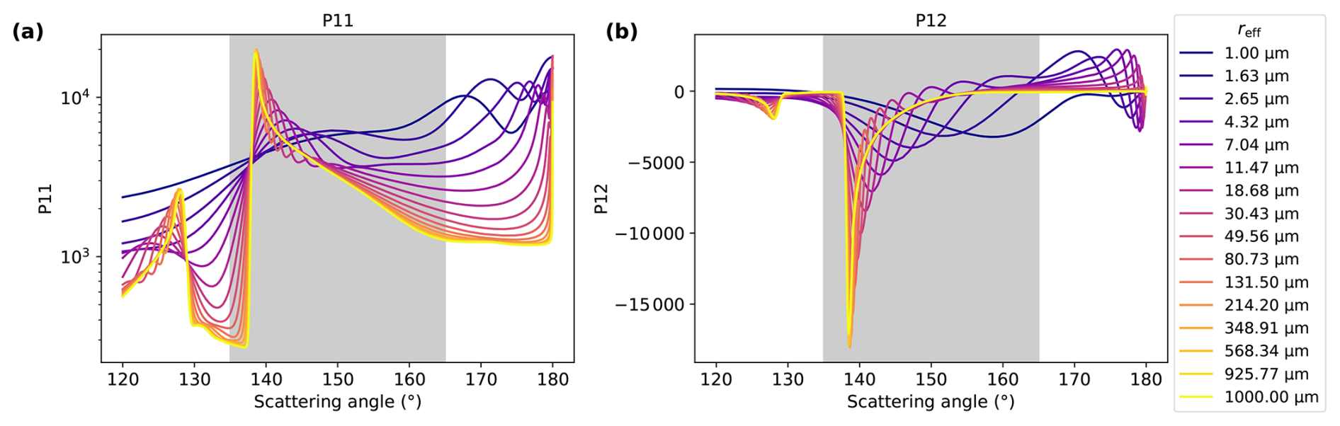
Figure 1 Phase matrix components P₁₁ in (a) and P₁₂ in (b) of the extended phase function table in the scattering angle range between 120 and 180° for different effective radii between 1 and 1000 µm and a constant effective variance of 0.1 integrated for the green channel of the polarization cameras of the specMACS instrument. The gray shaded area marks the scattering angle region between 135° and 165° where the polarimetric cloudbow retrieval is performed (Pörtge et al., 2023; Alexandrov et al., 2012a).

Figure 1 shows the phase matrix components P₁₁ and P₁₂ in the scattering angle range between 120° and 180° integrated for the green channel of the RGB polarization cameras of specMACS for an effective variance of v_eff=0.1 and different effective radii between 1 and 1000 µm (every 10th radius of the extended phase function table). The gray shaded area in both panels marks the region of the cloud- (and rainbow) between 135° and 165° scattering angles which has been used for the polarimetric retrievals of CDSDs (e.g,  Pörtge et al., 2023; Alexandrov et al., 2012a). It can be seen, that in particular the polarimetric phase functions P₁₂ split up in that regime for the different effective radii and the minimum moves towards lower scattering angles for larger effective radii. However, it also becomes clear that there is less sensitivity for larger effective radii. We will investigate this in more detail in Sect. 2.4. Next to the cloud- and rainbow, we can also see the second order rainbow as a secondary maximum in P₁₁ and a secondary minimum in P₁₂ between 120° and 130°, which becomes more pronounced for larger effective radii. In between the two rainbows, Alexander's dark band is clearly visible for larger radii. Around 180°, the backscatter glory can be identified, which has also been used for remote sensing of cloud droplet size distributions (Mayer et al., 2004).

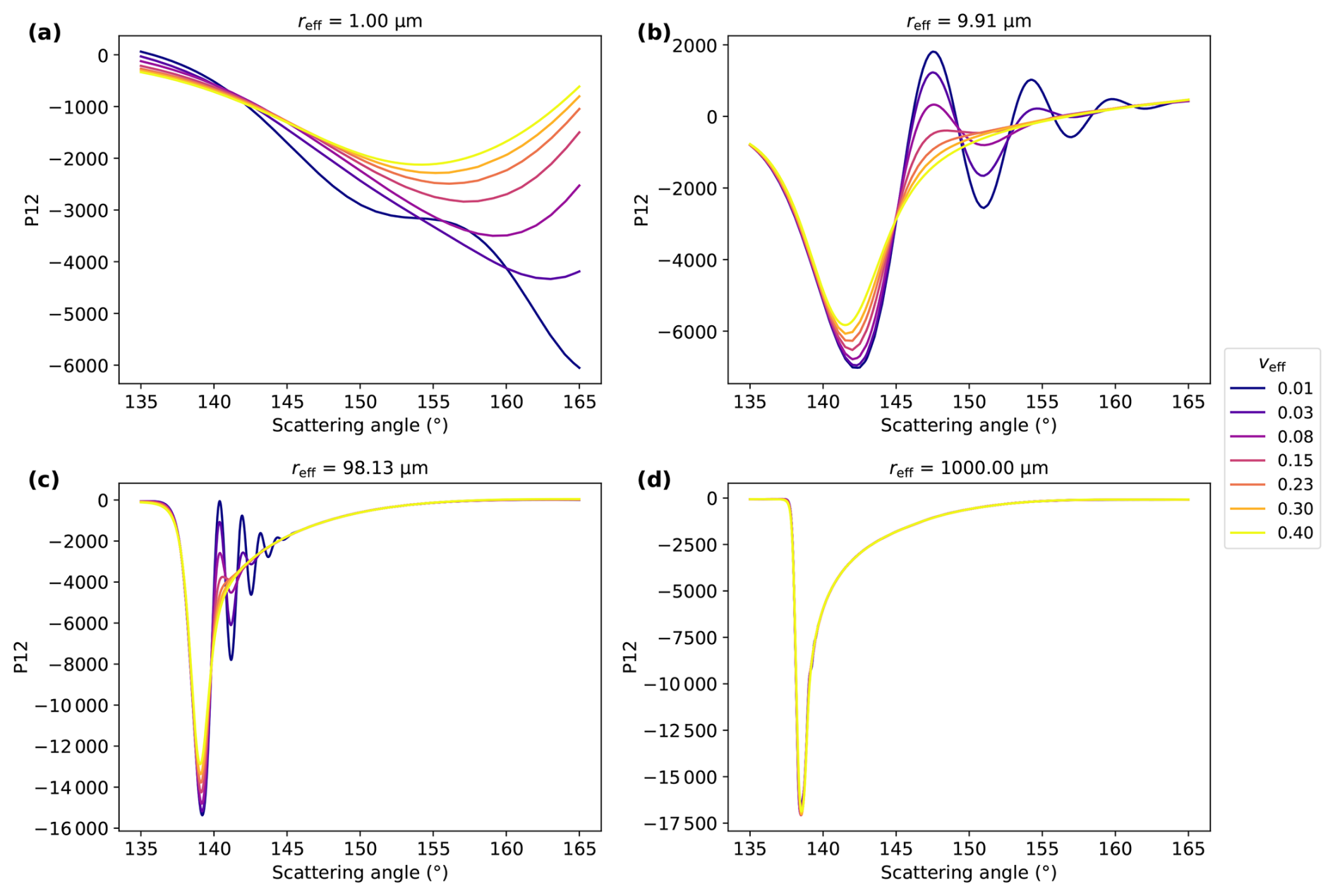
Figure 2 Dependence of the polarized phase function P₁₂ on the effective variance for four different effective radii: 1.00 µm (a), 9.91 µm (b), 98.13 µm (c), and 1000 µm (d).

Figure 2 shows the dependence of the polarized phase function P₁₂ on the effective variance for four different effective radii of 1.00 µm (Fig. 2a), 9.91 µm (Fig. 2b), 98.13 µm (Fig. 2c), and 1000 µm (Fig. 2d) in the cloud-/rainbow range between 135 and 165°. While the phase functions split up well for 1.00, 9.91, and 98.13 µm, hardly any difference can be seen for 1000 µm. For 9.91 and 98.13 µm, the polarized phase functions show next to the mostly aligned major minimum so-called supernumerary bows for the smaller effective variances. In contrast, the phase functions for 1.00 µm show significant differences between the effective variances as well, however, the minimum shifts clearly towards larger scattering angles for smaller effective variances. For v_eff=0.01, the major minimum is not even visible in the range of the cloudbow. Since shifts in the minimum occur also due to changes in the effective radius, there might be less sensitivity in the fit also for very small radii. Due to the indifference of P₁₂ for different effective variances at 1000 µm, it can be expected that large uncertainties in v_eff might occur at those values. As mentioned before, this will be investigated further in Sect. 2.4.

The motivation for the implementation of the multimode retrieval can be seen in Fig. 3. It illustrates the effect on the polarized phase function when two modes coexist in the droplet size distribution for a first mode with $r_{\text{eff},\mathrm{1}}=\mathrm{9.91}$ µm and a second one with $r_{\text{eff},\mathrm{2}}=\mathrm{98.13}$ µm. Different fractions that the individual modes contribute to the overall signal were chosen with $f_{\mathrm{1}}\in \mathit{\{}\mathrm{1.0},\mathrm{0.8},\mathrm{0.5},\mathrm{0.3},\mathrm{0.0}\mathit{\}}$ and $f_{\mathrm{2}}=\mathrm{1}-f_{\mathrm{1}}$. The existence of a second mode in the DSD changes the polarized phase function significantly, and hence would bias a retrieval that assumes a single mode gamma distribution.

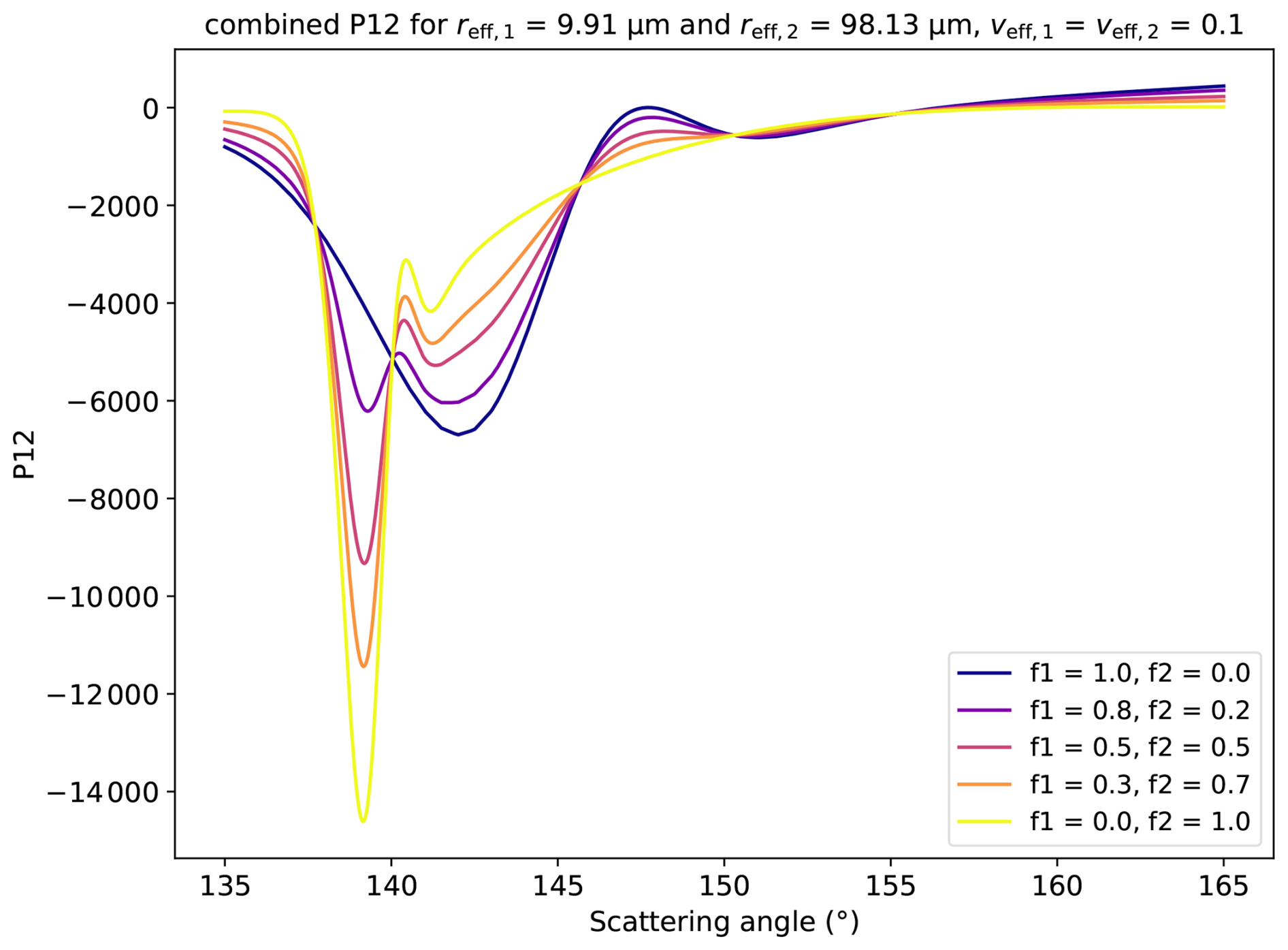
Figure 3 Effect of the coexistence of two modes in the droplet size distribution on the polarized phase functions for $r_{\text{eff},\mathrm{1}}=\mathrm{9.91}$ µm and $r_{\text{eff},\mathrm{2}}=\mathrm{98.13}$ µm. For both modes an effective variance of v_eff=0.1 was chosen. Different fractions for the individual modes were chosen with $f_{\mathrm{1}}\in \mathit{\{}\mathrm{1.0},\mathrm{0.8},\mathrm{0.5},\mathrm{0.3},\mathrm{0.0}\mathit{\}}$ and $f_{\mathrm{2}}=\mathrm{1}-f_{\mathrm{1}}$.

2.3 Retrieval algorithm

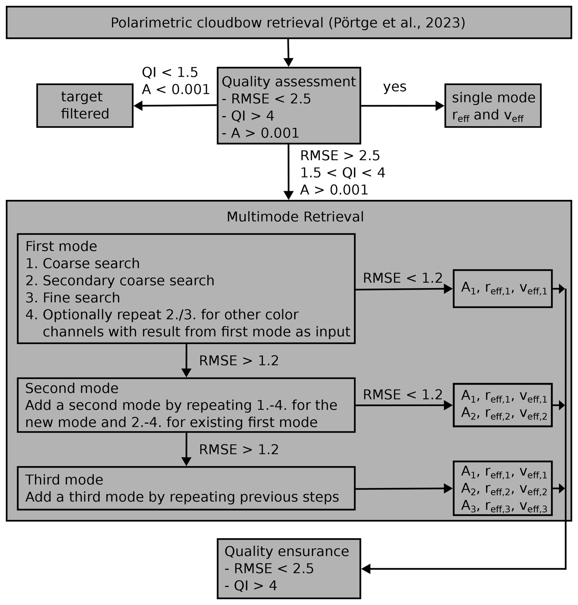
The retrieval algorithm is based on the aggregated angular radiance measurements in the scattering angle range between 135° and 165° described by Pörtge et al. (2023) and uses the single mode results as a starting point. The results from the single mode fit contain several quality measures which evaluate the quality of the fit (Pörtge et al., 2023): The root mean square error (RMSE, Eq. 7 in Pörtge et al., 2023)

$$\begin{array}{}\text{(22)}& {\displaystyle }\text{RMSE}=\sqrt{{\displaystyle \frac{\mathrm{1}}{N}}\sum _{i=\mathrm{0}}^n\left(Q_{\text{fit}}\right({\mathit{\theta }}_i)-Q_{\text{meas}}({\mathit{\theta }}_i){)}^{\mathrm{2}}}\end{array}$$

and the quality index (QI, Eq. 8 in Pörtge et al., 2023)

$$\begin{array}{}\text{(23)}& {\displaystyle }{\text{QI}}^{\mathrm{2}}={\displaystyle \frac{A^{\mathrm{2}}\left(〈P_{\mathrm{12}}^{\mathrm{2}}〉-\langle P_{\mathrm{12}}{\rangle }^{\mathrm{2}}\right)}{{\text{RMSE}}^{\mathrm{2}}}}.\end{array}$$

As in Eq. (9), θ denotes the scattering angle and A is the fit parameter that scales the polarized phase functions to the measured amplitude of the cloudbow. Cloud targets of the single mode fit results are not considered for further analysis, when RMSE>2.5 and QI<4 (Pörtge et al., 2023). Those targets, which do not fulfill the quality measures of the single mode fit are then used as an input for the multimode retrieval. However, targets where A<0.001 and QI<1.5 are not considered, since the signals do not contain a lot of information, e.g. due to ice, shadows or ocean influence.

While the single mode fit function from Eq. (9) has five free parameters for the fit (A, B, C, r_eff, and v_eff), every additional mode in the fit function after Eq. (11) adds another three free parameters to the parameter space, because the background B and C is fitted only once. Hence, it would be ambiguous to search the whole lookup table (LUT) for each mode and we decided on a strategy, which subsequently adds modes to the fit and searches the LUT in three different stages. First, an independent one-mode search is performed within the multimode retrieval by performing a coarse search through the LUT, which keeps every sixth effective radius and effective variance values. Since the fit is much more sensitive to r_eff than v_eff, we look for the best fitting effective radii for the central effective variance of the kept values first. The results for the five best effective radius fits are then combined with all possible effective variances to find again the five best candidates. Then, the fit is refined in a secondary coarse search around these best results from the first coarse search, which takes every second r_eff and v_eff in a window that includes the two neighbors of the coarsened LUT in both dimensions (r_eff and v_eff) around the found result into account. Again, the five best candidates from the second stage fit are kept, to perform a final search, which takes all candidates within a window of size two (±2 neighbors) around those results. Hereby, the result of the first mode found can be interpreted as the dominant mode generating the signal and does not resemble an average over the whole multimodal distribution, as already observed by Alexandrov et al. (2012a).

The result of the first mode serves as a starting point for sequentially adding up to a predefined maximum number of modes n_m. For the new mode, the fit strategy described above is repeated, while the results for the r_eff and v_eff of the single best fit from the preceding step are used as centers for local search windows. Hence, when adding a second mode, the possible r_eff and v_eff values of the coarsened LUT are combined with the neighboring values of the LUT of the best r_eff and v_eff of the first mode. For each combination, the fit parameters A_i, B, and C are refitted to minimize the objective function (here: RMSE), and the best result is kept to perform the secondary coarse search and the fine search with the newly added mode.

Modes are added until either the predefined maximum number of modes is reached or the newly obtained fit satisfies the RMSE threshold (currently 1.2) for all fitted color channels. A newly added mode is accepted only when the objective function does not worsen and the fitted mode amplitudes are positive for all fitted color channels. If the new fit worsens the objective for any of the color channels, the preceding best valid fit is retained.

Because different combinations of phase functions can produce similar angular radiance curves, the multimode inverse problem may admit several comparably good solutions. Hence, it should be mentioned that the result might describe a local minimum rather than the global minimum which could lead to errors in the resulting droplet size distributions. Further, the resulting solution is conditional on the LUT, search-window strategy, objective function, and positivity constraints. However, first applications of the current fit strategy show promising results, which are presented in Sect. 3.

Afterwards, the quality of the results of the multimode fit can still be ensured by applying a threshold filter as for the single mode retrieval. Next to the RMSE, we define the quality index QI for a multimodal fit analog to the quality index for the single mode fit from Eq. (23) as

$$\begin{array}{}\text{(24)}& {\displaystyle }\begin{array}{rl}{\text{QI}}^{\mathrm{2}}:=& {\displaystyle \frac{\text{Var}\left({\sum }_{i=\mathrm{1}}^M{A}_i{P}_{\mathrm{12}}^i\right)}{{\text{RMSE}}^{\mathrm{2}}}}\\ =& {\displaystyle \frac{〈{\left({\sum }_{i=\mathrm{1}}^M{A}_i{P}_{\mathrm{12}}^i\right)}^{\mathrm{2}}〉-{〈\left({\sum }_{i=\mathrm{1}}^M{A}_i{P}_{\mathrm{12}}^i\right)〉}^{\mathrm{2}}}{{\text{RMSE}}^{\mathrm{2}}}}.\end{array}\end{array}$$

Similar to the goodness thresholds for the single mode fit, we filter targets when RMSE<2.5 and QI>4. The individual steps of the retrieval algorithm and the fit strategy are summarized in Fig. 4.

Figure 4 Schematic overview of the retrieval algorithm and fit strategy.

2.4 Sensitivity of the single mode retrieval to large droplets

Figure 1 shows that the phase functions for larger droplets do not split up as much as the phase functions for the well tested smaller droplets in the cloudbow region. Hence, the first question to be answered is the sensitivity of the fit to larger droplets. To this end, we added random measurement noise equivalent to the noise in real measurements of the specMACS polarization cameras to the phase functions in the LUT and generated a data set which includes several targets for each (r_eff,v_eff) pair. The fit routine described in Sect. 2.3 was applied to the measurement resembling data set for a maximum number of modes n_m=1 allowing to test the sensitivity of a single mode fit dependent on the actual effective radius and variance. The results are shown in Fig. 5. In Fig. 5a, a larger spread of the derived effective radius can be seen both towards small effective radii smaller than about 2 µm and as expected also towards effective radii larger than about 200 µm. In Fig. 5b, the comparison between the actual input effective variance and the derived effective variance is plotted, showing a spread for all values. While the mean follows the 1:1 line well, a slight overestimation can be seen for small effective variances and an underestimation for larger effective variances, which is due to the end of the LUT. Further, it can be seen that the retrieved effective variances accumulate both in the smallest (v_eff=0.01) and the largest (v_eff=0.4) effective variance bins, which is mainly due to insensitivities of the phase functions for large effective radii as seen in Fig. 2.

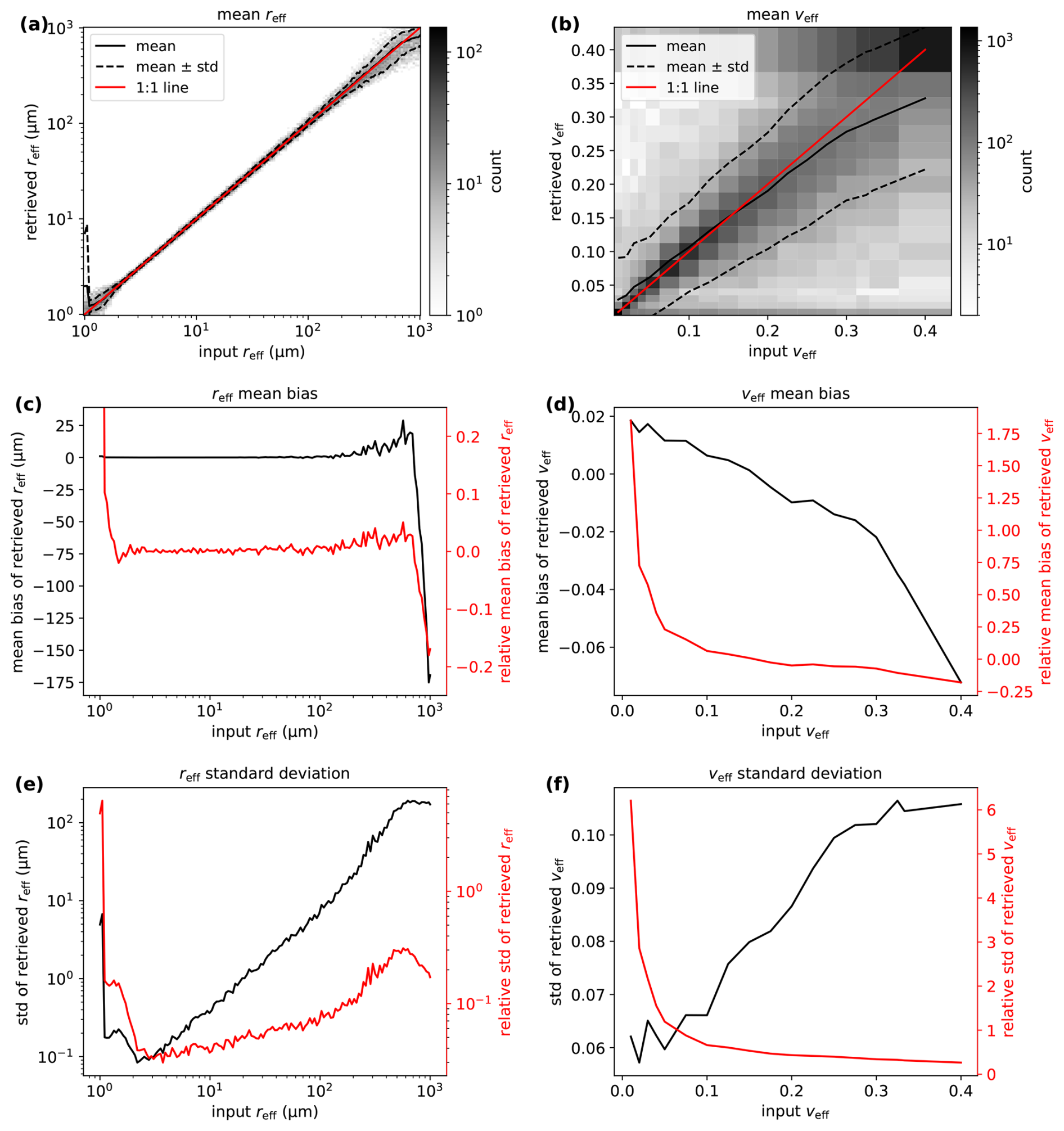
Figure 5 Sensitivity of the single mode fit with respect to the effective radius and the effective variance. In panel (a), the derived effective radius is plotted with respect to the actual input radius. The black line shows the mean radius derived for each input radius, while the two black dashed lines are the mean plus/minus the standard deviation of each interval. The red line denotes the 1:1 line. The same is shown for the effective variance in panel (b). In panels (c) and (d), the absolute mean bias is shown in black for each effective radius and variance respectively. In red, the relative mean biases are depicted. The same is shown for the standard deviation (black) and relative standard deviation (red) for the effective radius (e) and variance (f).

In Fig. 5c and d, the absolute (black, left axis) and the relative (red, right axis) mean biases are shown with respect to the input effective radius and variance respectively. The mean bias of the effective radius remains approximately zero for effective radii up to 200 µm which is consistent with the findings from Fig. 5a and also holds for the relative mean bias, although the relative mean bias is increased for r_eff<2 µm as seen before. For radii between 200 µm and about 700 µm, the mean bias increases to about +20 µm around 500 µm, before it falls off to negative values down to about −175 µm at 1000 µm. The overestimation for r_eff<2 µm and the underestimation for r_eff≳700 µm might also be related to the fact that they are close to the borders of the LUT, such that potential errors are always positive or respectively negative. Altogether, it can be concluded that the effective radius can be determined with an accuracy better than 10 % between about 1.5 µm and 800 µm and hence, fulfills the requirement determined by Mishchenko et al. (2004) for the r_eff of liquid droplet size distributions to monitor the long-term aerosol and cloud forcing from space. For the bias of the effective variance shown in Fig. 5d, a steady decrease towards larger v_eff can be seen. While the effective variance is overestimated for v_eff≲0.15, it is underestimated for values above 0.15. The overestimation at small effective variances results in a relative bias of up to about 2, with a fast decrease down to about 0.2 at v_eff=0.05. At the largest effective variance of v_eff=0.4 an underestimation of about −0.07 or −20 % is found. Again, it should be kept in mind that overestimates at small effective variances and underestimates at large v_eff might be caused by reaching the borders of the LUT. Compared to the accuracy requirements determined by Mishchenko et al. (2004) of 0.05 or 50 %, the requirements are met for all effective variances, either because of their low absolute or relative bias.

The same is shown for the standard deviation in Fig. 5e and f. As denoted before, the standard deviation of the derived effective radius is large for very small effective radii (r_eff≪2 µm), which is mostly due to single outliers. While it drops to a minimum of about 0.1 µm at r_eff≈3 µm, it steadily increases for larger r_eff up to nearly 200 µm for r_eff≳500 µm. However, this means that the relative standard deviation stays below about 0.4 for all r_eff except for the very small values close to about 1 µm. The standard deviation of the derived effective variance generally increases for larger input effective variances from about 0.06 to about 0.10 for v_eff≳0.3. However, the relative standard deviation steadily decreases for larger v_eff with values below 0.5 for v_eff≳0.15.

Volkmer et al. (2024b) performed an extensive study on the accuracy of the single mode polarimetric retrieval applied to measurements of the specMACS instrument using 3-D radiative transfer simulations of a field of shallow cumulus clouds. They found an uncertainty in the effective radius of $(-\mathrm{0.17}\pm \mathrm{1.30})$ µm, which corresponds to a relative mean bias of less than 2 % when compared to the average radius of 10.49 µm expected from the model data. While the values found were averaged for all effective radii between 1 µm and about 40 µm (the values included in the existing LUT for the single mode retrieval), they compare well to the values found from Fig. 5c. With regard to the effective variance, Volkmer et al. (2024b) found an uncertainty of (0.02±0.05), which corresponds to a relative mean bias of 15 % at an average expected effective variance of 0.14. Note that the simulations did not include any v_eff<0.1 as this was the effective variance assumed for each grid box of the model simulations. In contrast to the results from Fig. 5d, Volkmer et al. (2024b) found rather an overestimation in the effective variance. This might be explained by the idealized model that was used for this study, which includes typical measurement uncertainties with respect to the measured value of Q, and hence only indirectly includes errors that might occur for example due to cloud movements or uncertainties in the cloud top height.

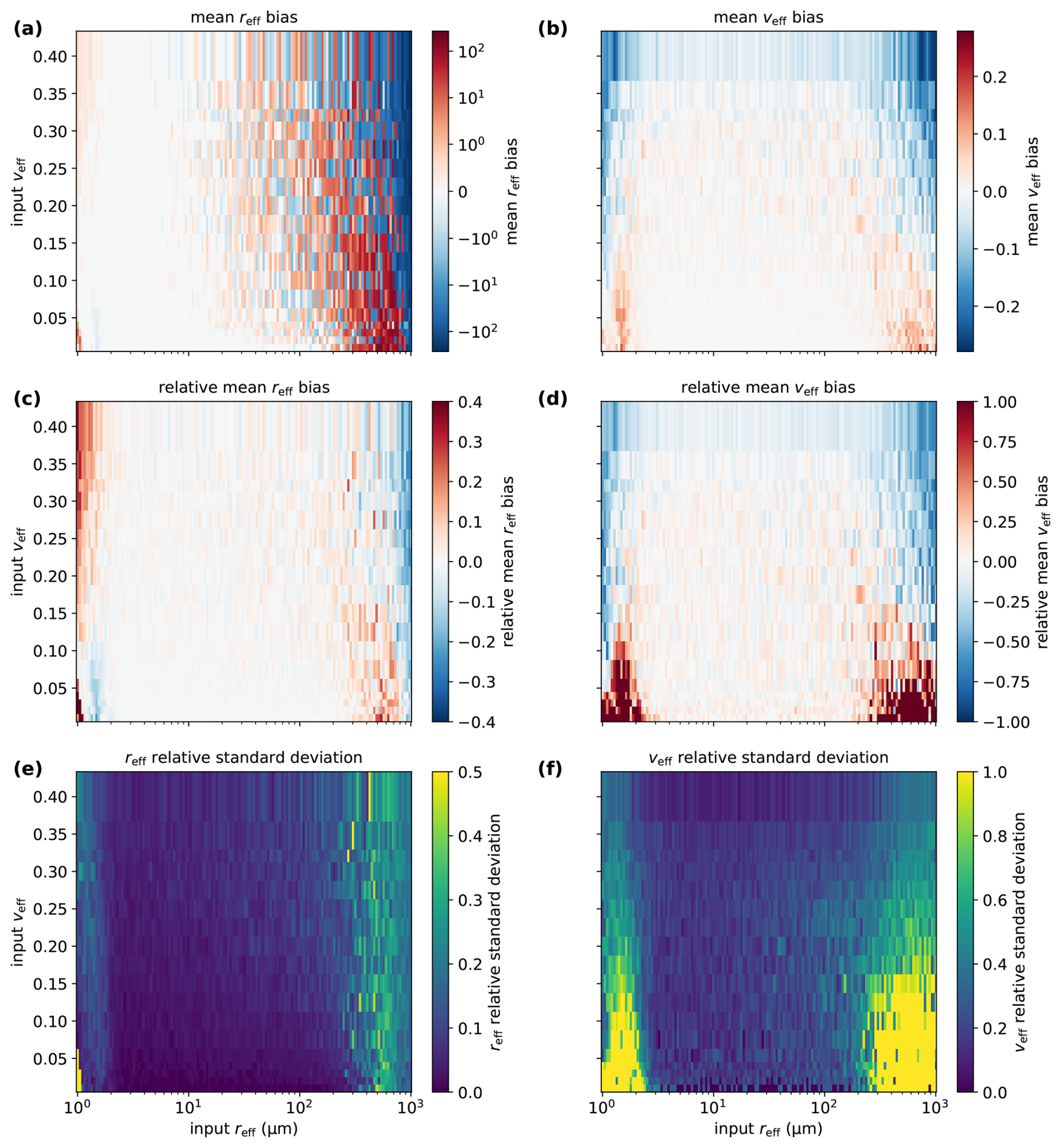
Figure 6 Sensitivity of the single mode fit with respect to the effective radius and the effective variance. In (a), the mean bias of the effective radius is plotted with respect to the input effective radius and variance. Overestimates are shown in red, while underestimates are shown in blue. The mean bias of the effective variance is depicted in panel (b). In panels (c) and (d), the relative mean bias is shown for the effective radius and variance respectively. Panels (e) and (f) illustrate the relative standard deviations.

Figure 6 illustrates the sensitivity of the single mode fit on both the effective radius and variance of the input. In Fig. 6a, the mean bias of the retrieved effective radius is shown with red values denoting an overestimation while blue regions show underestimates. Each pair of input (r_eff,v_eff) was calculated 12 times. As expected, larger uncertainties are found for larger input r_eff with both overestimates and underestimates occurring. However, overestimates tend to dominate in the beginning while underestimates take over the larger the effective radius, which might be due to the end of the LUT coming closer as discussed before. This shift from over- to underestimates tends to occur later for smaller effective variances, while the effective radii are mostly underestimated for the smallest effective variance of 0.01. Finally, the overestimation of the effective radius for small effective radii as seen already in Fig. 5a is also visible, with the largest overestimates occurring for small effective variances. Further slight overestimates can be seen for larger variances, while there is hardly any overestimation for medium effective variances between about 0.07 and 0.16. Figure 5c shows the relative mean bias for each pair of (r_eff,v_eff). As before, it is mostly well below 10 %, particularly for $\mathrm{2}\mathrm{\mu }\mathrm{m}\lesssim r_{\text{eff}}\lesssim \mathrm{200}$ µm and v_eff≲0.1. The corresponding relative standard deviation is shown in Fig. 6e. As stated above, most of the values are well below 0.5 except for very small effective radii smaller than 2 µm and low effective variances as well as single outliers at larger effective radii (≳200 µm).

The analog plots for the effective variance are shown in Fig. 6b, d and f. While large effective variances tend to be underestimated especially at very small effective radii (≲2 µm) and for large effective radii ≳200 µm, the opposite holds for small effective variances ≲0.1. Parts of this might be explained by the end of the LUT, although the determination of the effective variance works well in between except for slight overestimates for $\mathrm{0.15}\lesssim v_{\text{eff}}\lesssim \mathrm{0.25}$. This is reflected by the relative mean bias in Fig. 6d, with overestimates above 100 % occurring only for v_eff<0.1 and r_eff<3 µm or r_eff>200 µm. In between, slightly red colors seem to dominate except for v_eff≳0.27. This might explain the findings of Volkmer et al. (2024b), that the effective variance is overestimated while we found on average rather underestimates for v_eff≳0.12 from Fig. 5d, which seems to be dominated by the underestimates at very small and very large effective radii. The relative standard deviation in Fig. 6f shows a similar picture with large values occurring particularly at small and large effective radii. Hereby, values larger than 1 are found at small effective variances smaller than about 0.15 and for r_eff≲3 µm and r_eff≳200 µm. Hence, for those ranges the determination of the effective variance becomes highly uncertain, which is as expected from Fig. 2.

In conclusion, an accurate determination of the effective radius is still possible even for larger effective radii where the phase functions become less distinct, in particular with respect to the relative mean bias and standard deviation. For the effective variance larger uncertainties were found towards larger effective radii, and particularly small effective variances might be hard to determine.

3 Results

In the following section, we show a measurement example of a precipitating cumulus congestus observed on 7 September 2024 around 13:50 UTC with one of the polarization cameras of specMACS in the vicinity of Barbados during the PERCUSION campaign. Figure 7a shows the measured RGB image and Fig. 7b the degree of linear polarization (DOLP) as an RGB composite of the three color channels of the camera. Both panels contain a zoom into the region where the rainbow can be seen. While it is not easy to see in the normal RGB image, it becomes clearly visible in the RGB DOLP composite due to the shift of the minimum of the (polarized) phase function between the individual color channels and the much weaker background signal.

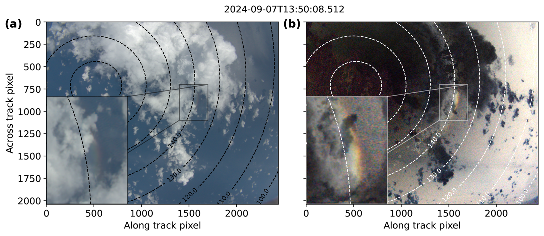
Figure 7 Measurement example of a raining cumulus cloud observed on 7 September 2024 around 13:50:08 UTC by the polarization camera of specMACS. In (a), the RGB image is shown. In (b), the RGB composite of the measured degree of linear polarization (DOLP) of the camera's three color channels can be seen. In the lower left of each subplot a zoom into the region where the rainbow can be seen is shown. The dashed lines denote the scattering angles of the observations.

Further evidence of rain within the observed cloud is found in the data of the 35.5 GHz cloud radar of the HAMP microwave package (Mech et al., 2014; Ewald et al., 2019), which was operated simultaneously to specMACS on board of HALO as part of the “cloud observatory” payload (Stevens et al., 2019; Konow et al., 2021). Figure 8 shows the maximum radar reflectivity projected to the specMACS polarization RGB image in Fig. 8a and the corresponding vertical cross section of the measured radar reflectivity in Fig. 8b. The measurements with the large reflectivities show clearly hydrometeors reaching the ground, and hence indicate the presence of rain. Of course it should be mentioned again, that specMACS does not penetrate through the cloud, but the sideward viewing geometry allows the observation of rain close to the cloud edges and in case of advection.

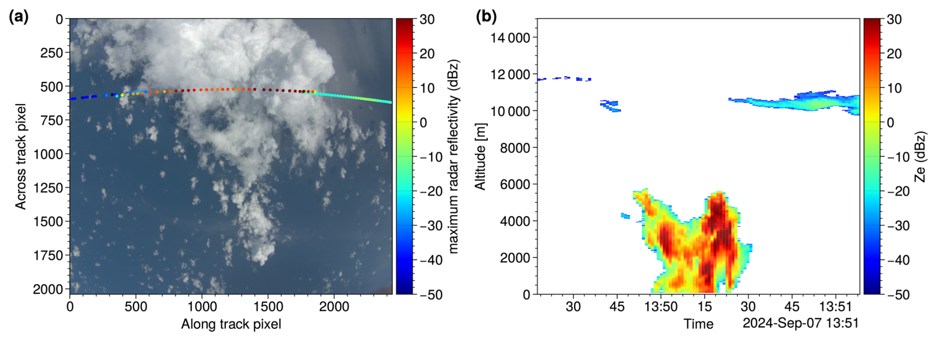
Figure 8 Measurements of the HAMP MIRA cloud radar of the raining cumulus cloud observed on 7 September 2024 around 13:50:08 UTC. In panel (a), the maximum radar reflectivity is shown for each point in time projected to the RGB image of the polarization camera of specMACS. In panel (b), the vertical cross-section of the radar reflectivity can be seen.

Figure 9 shows the (unfiltered) polarimetric single mode retrieval results. The interpolated cloud top height derived by the stereographic retrieval (Kölling et al., 2019; Volkmer et al., 2024a) depicted in Fig. 9b indicates cloud tops up to about 6000 m. The derived effective radius (Fig. 9c) and effective variance (Fig. 9d) are only available for a limited area which is the region of cloud targets which were observed under the required range of scattering angles between 135° and 165° such that the polarimetric single mode retrieval can be applied. The effective radius shows smaller values for lower cloud top heights, while the observed radii become generally larger at higher altitudes. Next to the region where the rainbow is observed, a clear signal of large effective radii at the end of the LUT (around 40 µm) can be seen. This may already indicate that the single-mode retrieval, and particularly its LUT, is not sufficient in this case. In Fig. 9e and f the quality measures of the single mode fit, namely the RMSE (Eq. 22) and QI (Eq. 23) respectively, are shown. Values that are outside the valid range for the single mode retrieval (RMSE>2.5 and QI<4) are marked in black. It can be seen that the region of larger effective radii close to the observed rainbow shows higher RMSE (although not all of the points fall outside the valid range) and in particular smaller QI values outside the valid range. This further indicates that the single mode fit does not sufficiently explain the observed polarized signal.

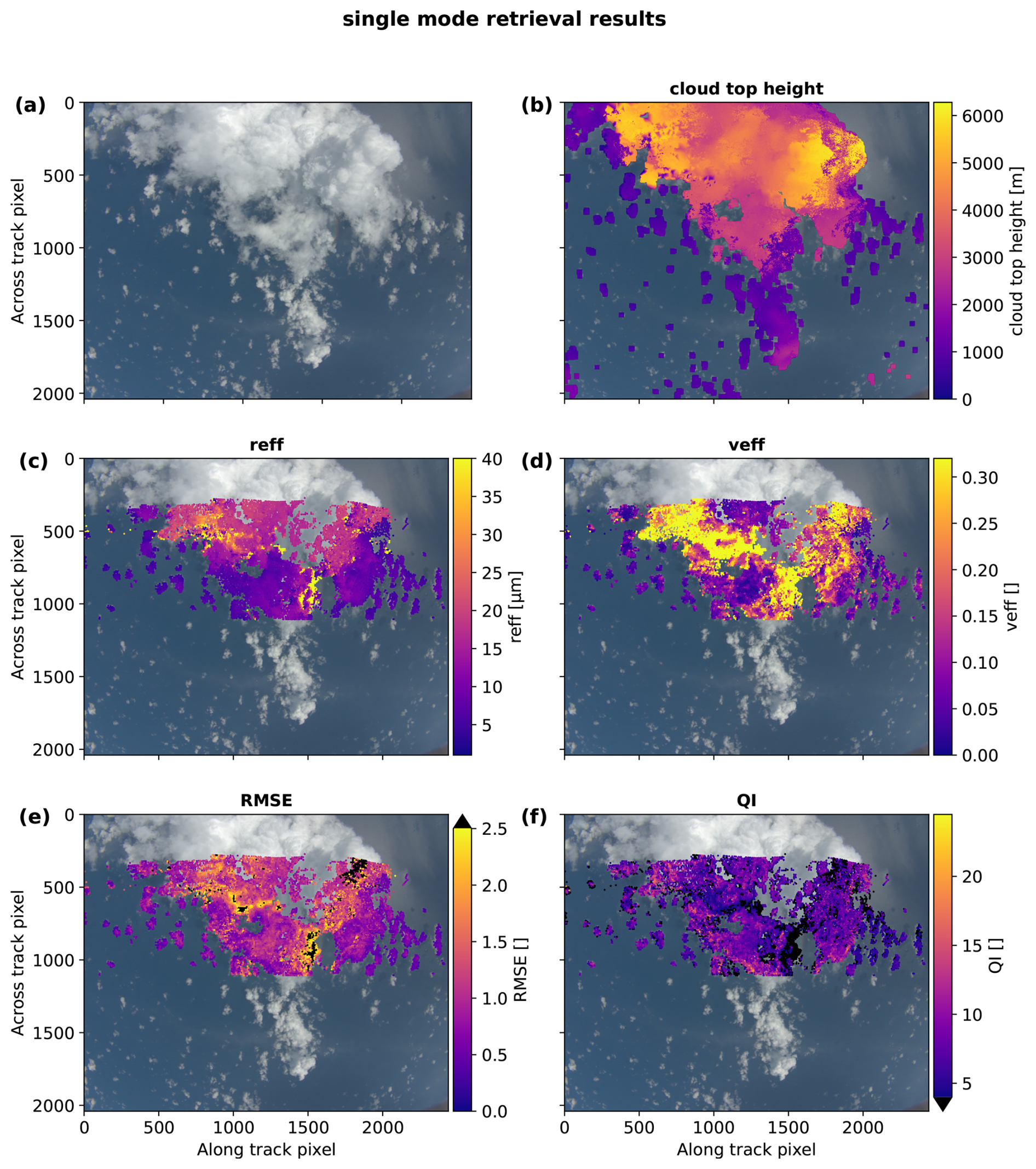
Figure 9 Results of the polarimetric single mode cloudbow retrieval for the measurement example of the raining cumulus cloud observed on 7 September 2024 around 13:50:08 UTC by the polarization camera of specMACS. Panel (a) shows the RGB image taken by the camera, while the cloud top height is projected to the image in panel (b). In panels (c) and (d), the derived effective radius and respectively variance can be seen. In panels (e) and (f), the RMSE and quality index of the single mode fit are shown. Targets with RMSE>2.5 and QI<4 are marked in black in the respective panel.

Those points are input to the multimode retrieval and Fig. 10 shows the results of the individual modes of the cloud targets. The points shown were filtered by the same thresholds as for the single mode retrieval: Points with RMSE>2.5 and QI<4 were filtered out to ensure the quality of the results. In Fig. 10a–c, the resulting effective radii are shown for the three modes, while Fig. 10d–f show the corresponding effective variances. Figure 10g–i show the signal fraction f_A as defined in Eq. (13), whereas Fig. 10j–l depict the corresponding droplet number concentration fraction f_N after Eq. (19). From Fig. 10a and b, we can see that the resulting effective radius for the two dominant modes occurs in patches of smaller and larger values and not randomly, which is a good initial indication of the credibility of the results. Most of the r_eff values of the dominant mode (Fig. 10a) are between about 10 and 100 µm, same for the second mode (Fig. 10b). Figure 10c shows on the other hand that there are mainly two regions that need a third mode for an accurate explanation of the signal: close to the observed rainbow and further towards the upper right of the image. Hereby, the resulting r_eff seem to be less structured, however, as pointed out in Fig. 10i, most of them contribute only with a few percent to the measured signal. Comparing Fig. 10a and b in more detail, it can be seen that the derived effective radii are to some extent complementary in a manner that when a larger r_eff (𝒪(100 µm)) is retrieved as the first mode, then a smaller r_eff (𝒪(10 µm)) is derived as the second mode and vice versa.

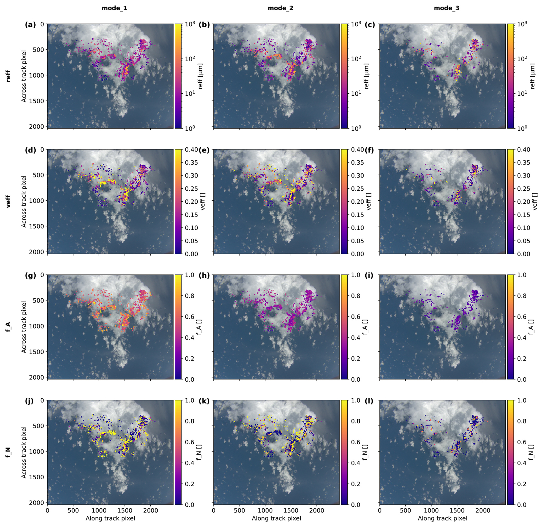
Figure 10 Results of the multimode approach for the measurement example of the raining cumulus cloud observed on 7 September 2024 around 13:50:08 UTC by the polarization camera of specMACS. The columns of the figure depict the individual modes, while the rows show the derived effective radius (a–c), the effective variance (d–f), the signal fraction f_A (g–i) and the droplet number concentration fraction f_N (j–l).

In contrast to the effective radius, the effective variance in Fig. 10d–f shows less structure, although not being completely random as well. This is expected, as it is in general harder to retrieve the effective variance correctly as shown in Figs. 5 and 6 and e.g. by Alexandrov et al. (2012a); Volkmer et al. (2024b).

Finally, comparing the signal fraction f_A in Fig. 10g–i to the droplet number concentration fraction f_N in Fig. 10j–l shows clearly that f_N is dominant for smaller effective radii independent of f_A. This is due to the proportionality of f_N to $\mathrm{1}/r_{\text{eff}}^{\mathrm{2}}$ as shown in Eq. (19).

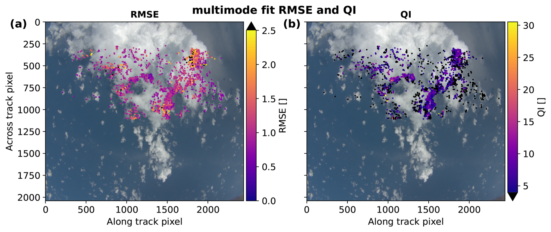
Figure 11 Quality measures of the multimodal fit results. In panel (a), the RMSE calculated after Eq. (22) of all points is projected to the RGB image of the polarization camera of specMACS. In panel (b), the corresponding plot is shown for the QI of the multimode fit calculated after Eq. (24). As for the single mode retrieval, points with RMSE>2.5 or respectively QI<4 are shown in black and mark the points which are filtered from the results of the multimode fit.

In Fig. 11, the resulting RMSE and QI of the multimode fit is shown for all points that were input to the multimode retrieval. Points that are filtered due to increased RMSE>2.5 or low QI<4 values are shown in black. While only a few black points occur in the RMSE plot, most points filtered are due to a low quality index as indicated by the black points in Fig. 11b. In total, we find for the example given here (so all points that are within the specMACS image shown) 2590 input targets to the multimode retrieval of which 62.5 % are valid. For the other targets, the signal is still not well explained even with several modes. A reason for this might be other uncertainties in the aggregation of the measured signal, e.g. due to the development of the cloud, convective movement, which is not captured in the mean wind from ERA5 data used in the single mode retrieval (Pörtge et al., 2023), or potential uncertainties in the cloud top height, which are needed for the correct identification of cloud targets in subsequent images. Further, 71.4 % of the valid targets have a RMSE less than 1.2, which is the threshold for adding a new mode. Together with the single mode retrieval, the example shown consists of 19246 cloud targets of which 80.4 % are valid with respect to the filters applied to the single mode retrieval results. Hence, with the multimode retrieval, we increase the number of valid targets to 88.8 %. Even though this corresponds just to an increase of about 8.4 %, we obtain valuable information about cloud microphysics, i.e. where multiple modes exist in the DSD and under which conditions they coexist. The improvement in the RMSE of the valid targets in the example compared to the RMSE of the single mode retrieval is on average 47.6 %, while we find an average increase of the QI of 145.0 %.

A remaining question to consider is whether large droplets can really be seen at the higher cloud tops as indicated by Figs. 10 and 9b. To this end, Fig. 12 combines the cloud targets from specMACS within the 1° cone around the radar beam with the radar measurements and optical thickness measurements of the WAter vapor Lidar Experiment in Space (WALES;  Wirth et al., 2009; Wirth and Groß, 2025). In Fig. 12a we show the radar reflectivity as in Fig. 8b, but this time overlayed with the cloud top heights (mean, minimum, and maximum) of the retrieved targets within the cone. The heights of the specMACS cloud targets are partly well below the radar heights (excluding the cirrus above), i.e. towards the upper left of the deeper convective cloud, which indicates that specMACS is sensitive to targets deeper within the cloud. The optical thickness at 532 nm measured by WALES is shown in Fig. 12b together with the corresponding cloud target heights, illustrating that the mean height of the retrieval points from specMACS is well in line with the attenuation of the lidar at optical thicknesses around one. Thus, this might be evidence that specMACS penetrates into the areas where the radar shows an enhanced reflectivity and large droplets might be present as the optical thickness above is low. In Fig. 12c, we show the corresponding effective radii derived for the up to three modes. The dominant mode depicted in red shows targets with values up to about 100 µm around 13:50 UTC, exactly where the mean of the specMACS cloud target heights coincides with the higher radar reflectivity.

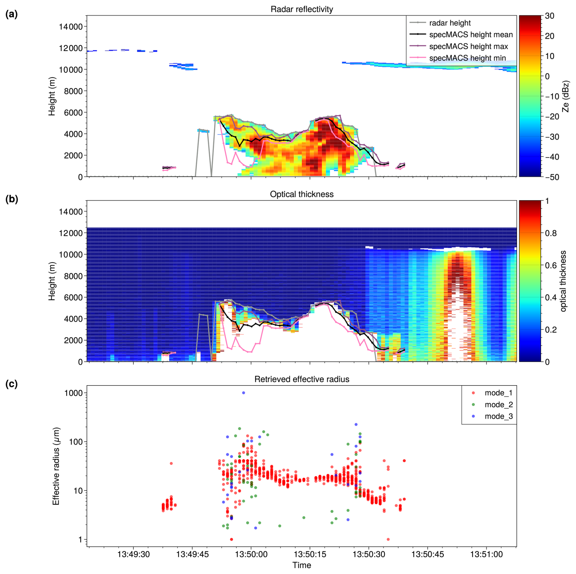
Figure 12 Timeline of the retrieval results within the 1° cone around the radar beam related to the radar reflectivity (a), and the optical thickness derived from lidar measurements (b). The retrieval results are shown for the individual modes in panel (c). In panels (a) and (b), the cloud top height of the radar (without cirrus) is shown in grey, together with the mean (black), the maximum (purple) and the minimum (pink) cloud top height of the specMACS cloud targets within the cone.

While the example shown gives an indication for the capability of the multimode fit retrieval to derive the individual parameters of the CDSD of cloud targets consisting of a superposition of multiple gamma distributions, a more qualitative comparison of the resulting fit of individual targets to the measured signal, the original result of the single mode fit and the Rainbow Fourier Transform (RFT, Alexandrov et al., 2012b) will be given in the next section.

3.1 Evaluation of single targets and comparison to RFT

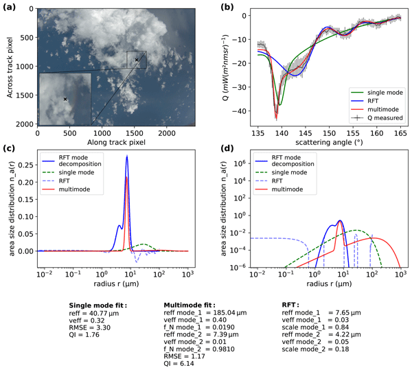
As shown in the previous section, the effective radius of the multimode retrieval shows some systematic patterns for the derived modes, which hints towards a stable retrieval algorithm. To further evaluate the results, we compare the results for four individual targets in Figs. 13–16 to the original result of the single mode fit and the RFT. All four figures show the location of the target in panel (a), and the measured signal, the resulting multimode fit as well as the single mode fit result and RFT fit result in panel (b). The RFT fit result is computed from the result of the mode decomposition after Alexandrov et al. (2015) as

$$\begin{array}{}\text{(25)}& {\displaystyle }\begin{array}{rl}{Q}_{\text{fit,RFT}}=& A_{\text{RFT}}\sum _{i=\mathrm{1}}^M{\mathit{\zeta }}_i\times P_{\mathrm{12}}^i[r_{\text{eff},i},v_{\text{eff},i}]\left(\mathit{\theta }\right)\\ & +B_{\text{RFT}}\times {\cos }^{\mathrm{2}}\left(\mathit{\theta }\right)+C_{\text{RTF}},\end{array}\end{array}$$

where ζ_i is the percentage scale of each mode derived from the mode decomposition and the parameters A_RFT, B_RFT and C_RFT are derived from a least-squares fit to the measurements, which makes the results of the RFT and the multimode retrieval comparable as best as possible. Panels (c) and (d) show the resulting so-called area size distributions of the single mode, and the multimode fit results as well as the distributions derived by the RFT and the corresponding mode decomposition. The area size distribution is hereby defined by Alexandrov et al. (2012b) as

$$\begin{array}{}\text{(26)}& {\displaystyle }{n}_a\left(r\right)={\displaystyle \frac{r^{\mathrm{2}}n\left(r\right)}{{\int }_{\mathrm{0}}^{\mathrm{\infty }}{r}^{\mathrm{2}}n\left(r\right)\mathrm{d}r}},\end{array}$$

where n(r) is the droplet size distribution as in Eq. (6). As the area distribution defines another gamma distribution which can be described in the same form as in Eq. (6), the “effective radius” and “effective variance” of the area distribution r_eff,a and respectively v_eff,a can be derived from the effective radius and variance of the droplet size distribution as

$$\begin{array}{}\text{(27)}& {\displaystyle }{r}_{\text{eff},a}=r_{\text{eff}}(\mathrm{1}+\mathrm{2}{v}_{\text{eff}})\text{and}{v}_{\text{eff},a}={\displaystyle \frac{v_{\text{eff}}}{\mathrm{1}+\mathrm{2}{v}_{\text{eff}}}}.\end{array}$$

The corresponding inverse transformation is given by

$$\begin{array}{}\text{(28)}& {\displaystyle }{r}_{\text{eff}}=r_{\text{eff},a}(\mathrm{1}-\mathrm{2}{v}_{\text{eff},a})\text{and}{v}_{\text{eff}}={\displaystyle \frac{v_{\text{eff},a}}{\mathrm{1}-\mathrm{2}{v}_{\text{eff},a}}},\end{array}$$

allowing to calculate the one distribution from the parameters of the other. Panels (c) and (d) differ from each other as we used a logarithmic scale in panel (d) to eventually show the multimodal structure more clearly, as larger cloud droplets are suspect to much lower cloud droplet number concentrations.

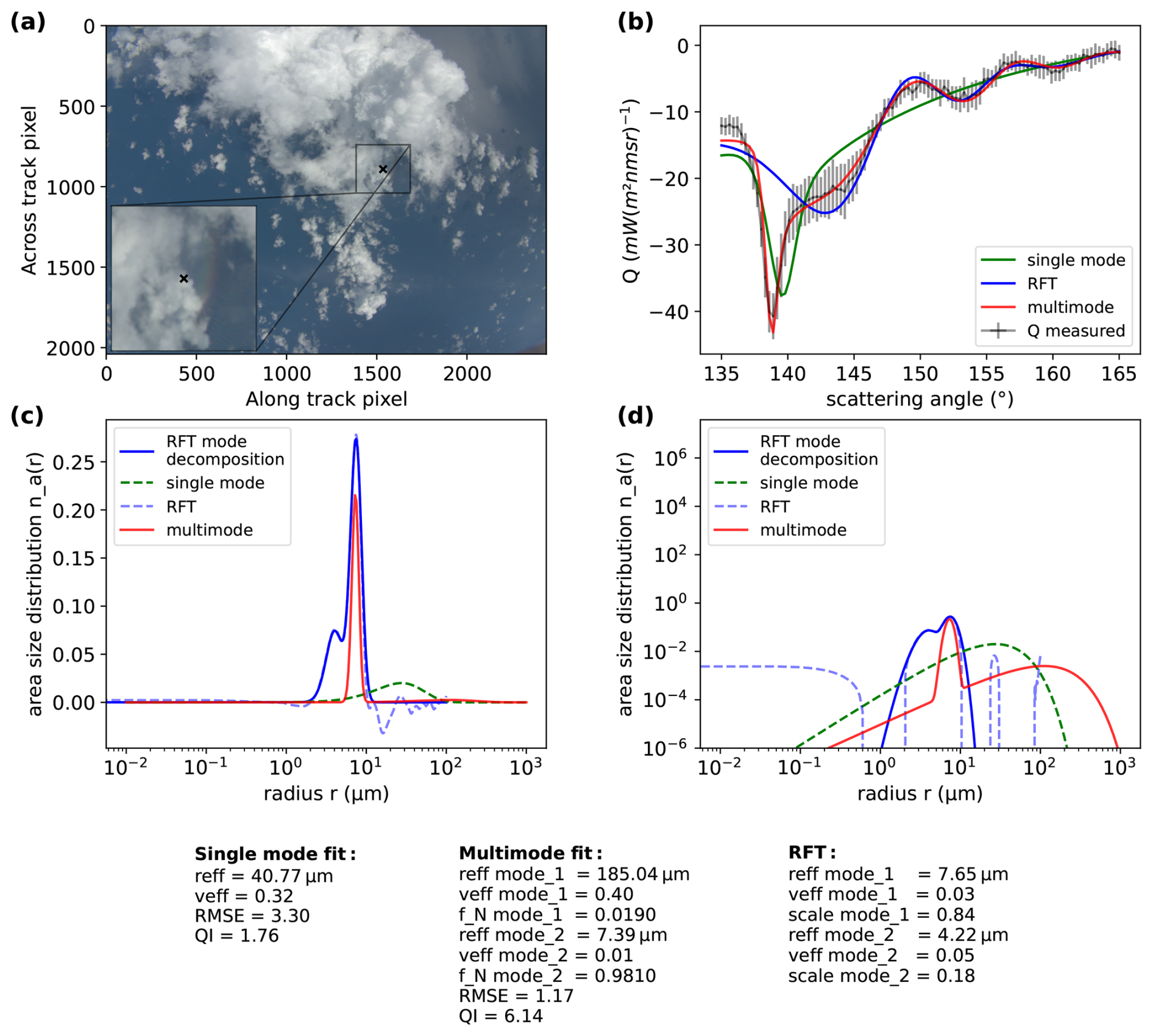
Figure 13 Retrieval results for an individual cloud target. The location of the target with respect to the image taken by the specMACS polarization camera taken around 13:50:08 UTC on 7 September 2024 is shown in panel (a). In panel (b), the measured Q component of the stokes vector is shown (grey with errorbars), the resulting fit of the multimode retrieval (red) as well as the original single mode fit (yellow) and the RFT mode decomposition result (blue) is shown. In panels (c) and (d), the corresponding area distributions derived from the retrievals are shown without and with a logarithmic scale of the y-axis.

In Fig. 13, the measured polarized radiance (Fig. 13b) and the results from the multimode fit (red), the RFT (blue) and the single mode fit (green) are shown for a cloud target located within the region close to the observed rainbow, where at least two modes were found in the shown figures in Sect. 3. This example shows a double cloudbow as obtained from the combination of phase functions shown in Fig. 3. Furthermore, we can observe two supernumerary minima, which hints to at least one mode with a narrow DSD, which is also what we find both from the multimode fit and the RFT: The multimode fit sees two modes, a signal dominating one with $r_{\text{eff},\mathrm{1}}=\mathrm{185}$ µm and a second one with $r_{\text{eff},\mathrm{2}}=\mathrm{7.39}$ µm. While the first mode is broad ($v_{\text{eff},\mathrm{1}}=\mathrm{0.4}$), the small droplet mode has a narrow distribution with $v_{\text{eff},\mathrm{2}}=\mathrm{0.01}$ explaining the supernumerary bows. From Fig. 13b, it can be seen that the found combination explains the measured signal very well with a RMSE of 1.17. The mode decomposition of the RFT on the other hand, finds a first mode that is with $r_{\text{eff},\mathrm{1}}=\mathrm{7.65}$ µm and $v_{\text{eff},\mathrm{1}}=\mathrm{0.03}$ very similar to the small droplet mode found from the multimode fit. It further finds a second mode with even smaller droplets and $r_{\text{eff},\mathrm{2}}=\mathrm{4.22}$ µm and $v_{\text{eff},\mathrm{2}}=\mathrm{0.05}$. Figure 13c hereby reveals, that both retrieval results find a distribution with a narrow peak around 7 µm, where both distributions are well aligned. In contrast, the multimode retrieval does not retrieve the secondary peak towards the left of the main peak of the RFT distribution, while Fig. 13d shows that the underlying broader distribution with its maximum around 150 µm is missed by the RFT. This is due to the fact that the RFT in its current implementation only retrieves radii up to 100 µm in the area size distribution, which means that the effective radii retrieved from the mode decomposition are in general lower than 100 µm. Moreover, the mode decomposition technique finds peaks in the area size distribution, but since droplet number concentrations are usually much smaller for larger droplets as can be seen from the distribution retrieved from the multimode retrieval in Fig. 13c, peaks at larger droplets might also be missed in general by the method. From Fig. 13c and d, we can also see one issue, that we usually observe when applying the RFT to specMACS measurements: the derived area size distribution shows negative values which are not removed by the corrections described by (Alexandrov et al., 2012b) making the results at least partly physically unrealistic.

Figure 14 Same as in Fig. 13 but for another cloud target.

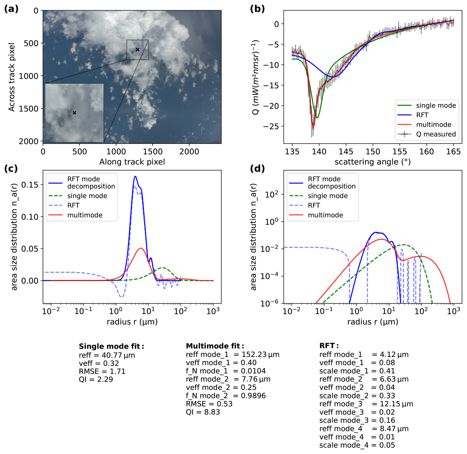
The results of the cloud target in Fig. 14 also show a clear multimodal structure as the target in Fig. 13. In Fig. 14b, we can clearly see that the signal is well explained by the new multimodal fit (red), while the single mode fit does not capture the measured signal properly. Here, the multimode fit finds two modes with $r_{\text{eff},\mathrm{1}}=\mathrm{152}$ µm and $r_{\text{eff},\mathrm{2}}=\mathrm{7.76}$ µm. Again, the first mode is broad with an effective variance of $v_{\text{eff},\mathrm{1}}=\mathrm{0.4}$, while this time, also a broader distribution of the second mode is found with $v_{\text{eff},\mathrm{2}}=\mathrm{0.25}$. From the single mode retrieval, a radius of r_eff,max=40.77 µm is found, which is consistent with the maximum radius of the LUT. The RFT finds four modes from the mode decomposition with effective radii $r_{\text{eff},\mathrm{1}}=\mathrm{4.12}$ µm, $r_{\text{eff},\mathrm{2}}=\mathrm{6.63}$ µm, $r_{\text{eff},\mathrm{3}}=\mathrm{12.15}$ µm and $r_{\text{eff},\mathrm{4}}=\mathrm{8.47}$ µm. This results in a fit calculated after Eq. (25) that seems to capture the lower effective radius mode well, while it does not explain the signal originating from the large droplets. Here, Fig. 14d makes clear that the RFT misses droplets larger than 100 µm where currently the definition of the RFT ends.

Figure 15 Same as in Fig. 13 but for another cloud target.

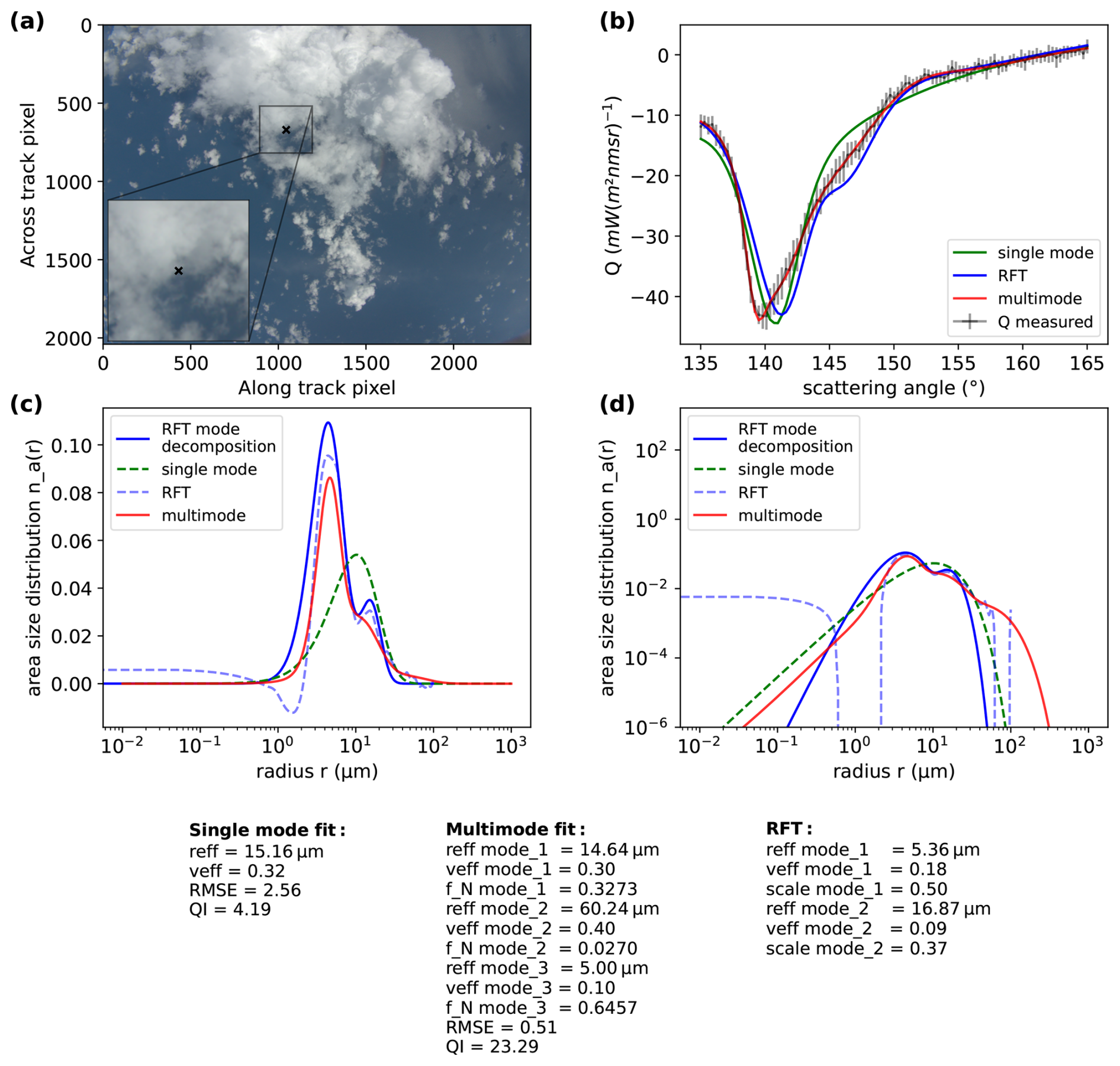
The example shown in Fig. 15 shows the capability of the multimode retrieval to explain the measured signal with three modes: One with $r_{\text{eff},\mathrm{1}}=\mathrm{14.64}$ µm and an effective variance of 0.30, a second one with an effective radius of 60.24 µm and an effective variance of 0.4 and one with $r_{\text{eff},\mathrm{3}}=\mathrm{5.00}$ µm and $v_{\text{eff},\mathrm{3}}=\mathrm{0.1}$. Altogether, the measured signal is described with a RMSE of 0.51 and a high quality index of 23.29 is found. In comparison, the mode decomposition from the RFT finds two modes, a first mode with $r_{\text{eff},\mathrm{1}}=\mathrm{5.36}$ µm and $v_{\text{eff},\mathrm{1}}=\mathrm{0.18}$, which is on the same order of the third mode found by the multimode and a second mode with $r_{\text{eff},\mathrm{2}}=\mathrm{16.87}$ µm and $v_{\text{eff},\mathrm{2}}=\mathrm{0.09}$. The resulting DSDs in Fig. 15c and d show that the DSDs of the RFT and the multimode retrieval are very similar. The major peak around 5 µm is both found by the RFT and the multimode retrieval and both distributions show a tail towards larger droplets, although the small peak around 11 µm is not as pronounced in the multimode retrieval as in the RFT. As before, the signal computed by the mode decomposition result does not describe the actual measured signal completely, which is most likely due to the missing contribution from the mode around 60 µm. This mode derived by the multimode retrieval is not encountered by the mode decomposition of the RFT, since droplet numbers are too small compared to the smaller droplets. In this example, the single mode fit does not hit the maximum effective radius of the LUT, but finds an effective radius of 15.16 µm. This corresponds to a combined effective radius which lies in between the 14.64 µm found by the multimode retrieval and the 16.87 µm of the RFT.

Figure 16 Same as in Fig. 13 but for another cloud target.

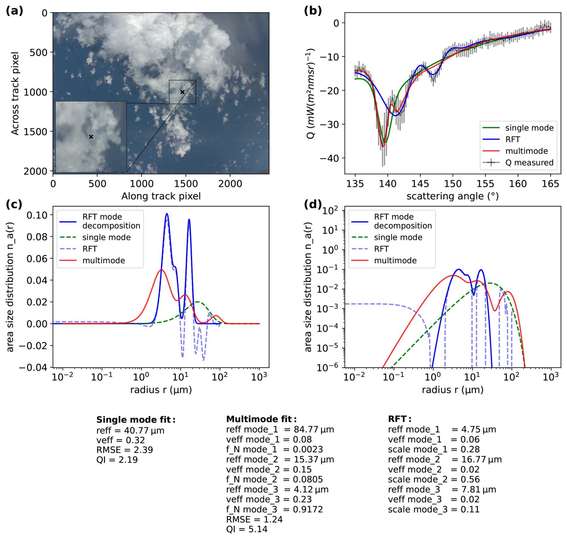
Figure 16 shows an example target, where the RFT captures the supernumerary bows of the measured signal very well, while the multimode retrieval fits the main minimum and the second minimum but not the supernumerary bows. Hereby, the mode decomposition of the RFT finds three modes, each with a rather small distribution: A first mode with $r_{\text{eff},\mathrm{1}}=\mathrm{4.75}$ µm and $v_{\text{eff},\mathrm{1}}=\mathrm{0.06}$, a second one with $r_{\text{eff},\mathrm{2}}=\mathrm{16.77}$ µm and $v_{\text{eff},\mathrm{2}}=\mathrm{0.02}$, and a third one with $r_{\text{eff},\mathrm{3}}=\mathrm{7.81}$ µm and $v_{\text{eff},\mathrm{3}}=\mathrm{0.02}$ are found. This explains that the supernumerary bows are fitted well by the RFT, while on the other hand, the multimode fit finds three modes as well with $r_{\text{eff},\mathrm{1}}=\mathrm{84.77}$ µm and $v_{\text{eff},\mathrm{1}}=\mathrm{0.08}$, a second one with $r_{\text{eff},\mathrm{2}}=\mathrm{15.37}$ µm and $v_{\text{eff},\mathrm{2}}=\mathrm{0.15}$, and a third one with $r_{\text{eff},\mathrm{3}}=\mathrm{4.12}$ µm and $v_{\text{eff},\mathrm{3}}=\mathrm{0.23}$. While the effective radii of both second modes are similar, the effective variance of the multimode fit is larger. This holds in general for all three modes and might explain why the multimode fit does not capture the supernumerary bows. Again, the RFT mode decomposition is subject to smaller effective radii and does not find the larger mode with an effective radius of about 84 µm, which explains why the fit does not capture the major minimum. Furthermore, the single mode retrieval is again biased towards larger radii and finds the maximum effective radius of the LUT with r_eff,max=40.77 µm and a broad distribution (v_eff=0.32). Figure 16c and d show, that the resulting size distributions differ between the different methods, although both the multimode distribution and the distribution from the RFT show three maxima, but they are shifted. One explanation for the deviation of the methods might be the noise of the measured data in Fig. 16b, which could be related to errors in the tracking of the target and hence, errors in the retrievals.

4 Discussion and Conclusion

In this work, we presented a new technique that builds on existing retrievals of cloud droplet size distributions using polarized measurements of the cloudbow, but takes more than one mode into account. The existing polarimetric CDSD retrievals are constrained to single mode gamma distributions with maximum effective radii of about 40 µm used by Pörtge et al. (2023) for the specMACS measurements. For POLDER, Shang et al. (2019) use a LUT with effective radii between 3 µm and 25 µm, while Alexandrov et al. (2015) use a table with effective radii between 5 µm and 30 µm for the RSP retrieval, and the LUT for the evaluation of the AirHARP measurements includes effective radii ranging between 5 and 20 µm (McBride et al., 2020). We extended the existing LUT used by Pörtge et al. (2023) to an effective radius of 1000 µm and showed, based on a measurement example from the PERCUSION campaign, that this is necessary to be able to describe the measured signal in deep convective clouds. It was shown that despite the increasing similarity of the polarized phase functions towards higher effective radii, an estimate of the effective radius is still possible with a relative mean absolute bias of less than 10 % for a broad range of effective radii between about 1.5 µm and 800 µm (compare Fig. 5c) considering the measurement uncertainty of the specMACS cameras. This is the required relative accuracy to measure aerosol and cloud forcings in climate change from space according to Mishchenko et al. (2004). The standard deviation increases for larger radii with a maximum occurring around 500 µm of about 30 %. Only r_eff≲1.5 µm show even larger standard deviations. In terms of the effective variance, an increase in the mean bias and standard deviation towards small effective variances was found, particularly at very small (<3 µm) and large effective radii ≳200 µm. Nonetheless, the absolute mean bias of v_eff was found to be less than 50 % for v_eff≳0.03. We assumed a simple model for the measurement uncertainty which describes the variability in Q in dependence of Q itself. Hence, possible uncertainties in the signal aggregation process, e.g. due to wrong cloud top height estimates, convective cloud movements which are not described by the mean wind field estimate of the ERA5 data (Hersbach et al., 2020), or other biases in the aggregated signal in real measurements, such as shadows within the target region or ocean signals, were not taken into account. Studying how the existence of multiple modes affects the accuracy of the cloud droplet size distribution retrieval is subject to further studies.

Further uncertainties in the retrieval of larger effective radii might also be introduced by the implicit assumption of spherical droplets with the calculation of the scattering phase matrix elements using Mie theory. The shape of water droplets is spherical for radii up to about 400−500 µm, while they are described by spheroids in the radius range up to about 1 mm (Sect. 2.1.6 of Pruppacher and Beard, 1970; Beard and Chuang, 1987; Chuang and Beard, 1990). The deviation from spheres further increases for even larger droplets. First studies investigated the influence of the shape of rain droplets on the phase function compared to perfect spheres. For example, Macke and Großklaus (1998) used geometric optics for the phase function calculation of typical rain droplet size distributions and investigated the influence on the backscatter properties for lidar applications. Sadeghi et al. (2012) performed simulations of rainbows for non-spherical particles. However, they considered homogeneous size distributions only. The influence of non-spherical particles on the phase functions used in this work and possible implications on the derivation of size distributions from polarized measurements of the cloudbow will be investigated in the future.

Nonetheless, a conceptual framework of this new approach towards the retrieval of multimodal size distributions was given, and first results indicate the capability of the new fitting strategy based on a real measurement example. It could be seen that close to a rainbow observed in the measurements, a significant amount of targets show results with more than one mode. Moreover, the results included at least one mode with effective radii on the order of 100 µm, indicating that the observation included a signal originating from larger droplets as expected from the observation of the rainbow in the RGB image and simultaneous radar measurements. While this does not proof the overall concept of the method, examples of individual targets were shown that revealed that in most cases the measured polarized radiance signal is well explained by the multimode fit with up to three modes. Altogether, the single mode fit and the multimode fit are capable of explaining the measured polarized radiance signal of about 88.8 % of the cloud targets in the example considered, which is an increase of about 8.4 % compared to the single mode fit only. The targets improved by considering multiple modes showed an average decrease in the RMSE of about 48 % compared to the RMSE of the single mode fit. Further, an average increase in the QI of about 145 % was found.

Moreover, the results of the multimode fit were compared qualitatively for individual targets to the results of the CDSD independent approach of the Rainbow Fourier Transform described by Alexandrov et al. (2012b). The advantage of the RFT is that it does not need an a priori assumption about the size distribution, which, on the other hand, may lead to non-physical results like negative values. Nevertheless, in most cases the DSDs from the RFT and the multimode fit are similar, i.e. that one or several maxima of the distribution are recognized by both retrievals or that one mode found by one of the retrievals encloses the distribution of the other to some part. An improved agreement could e.g. be achieved by extending the RFT beyond 100 µm.

In the future, the uncertainty with respect to multiple modes will be investigated both in terms of 1-D and realistic 3-D simulations. Further, the retrieval will be applied to all measurements of the PERCUSION campaign and evaluated with regard to microphysical processes such as precipitation initiation under different meteorological conditions.