Evaluating low-cost NDIR CO₂ sensors for atmospheric observations in rural settings

Most research and monitoring activities involving low-cost atmospheric sensors (LC) have traditionally focused on urban environments, where air quality is a pressing concern. However, an emerging area of research is their application in rural landscapes, where land use is a key determinant of climate change and net zero outcomes, directly influencing greenhouse gas emissions, carbon sequestration, and ecosystem functioning. In this study, we examine the use of LC non-dispersive infrared (NDIR) CO₂ sensors to monitor atmospheric mixing ratios in agricultural settings. We present a data analysis framework that addresses errors associated with factory auto-baseline correction and, crucially, accounts for the influence of environmental parameters such as temperature and pressure. This approach leads to improved sensor performance. Results from deployments in both rural and urban environments demonstrate strong agreement with reference-grade instruments, as shown by the root mean square error (RMSE) and coefficient of determination (R²). Improvements of RMSE from 10 to 4 ppm in winter and 5 to 4 ppm in summer, with corresponding improved R² from 0.85 to 0.98 in winter and 0.86 to 0.97 in summer were obtained when compared to a simple scaling correction of the out-of-box data. Our study shows that corrected data not only reproduced the seasonal profile associated with rural emissions, but it also captured the diurnal variability, sometimes characterised by CO₂ change of up to 50 ppm, which is more than three times the typical change in the urban environment (15 ppm). Overall, this study establishes that field calibrated low-cost CO₂ sensors and sensor networks can provide reliable, long-term atmospheric monitoring in rural environments when sensor enclosures are appropriately designed to ensure adequate ventilation and air exchange, thereby preventing moisture accumulation. The observations obtained provide valuable inputs for developing analytical methodologies and offer actionable insights into the influence of rural land-use practices on climate.

1 Introduction

Carbon dioxide (CO₂) is a greenhouse gas that drives the warming of Earth's climate. The United Nations Sustainable Development Goals and the Intergovernmental Panel on Climate Change (IPCC) state that CO₂ emissions must be drastically reduced by 2030 to prevent atmospheric warming above 1.5 °C (IPCC, 2018). This goal requires both international collaboration and effective monitoring technologies to collectively reduce carbon emissions. CO₂ measurements can be used to estimate emission rates (Martin et al., 2017) but have historically been limited by the high cost of necessary instrumentation.

In recent years, technological advancements in low-cost sensors (LC) have enabled wider air quality monitoring and are increasingly being applied to greenhouse gas observations (Dubey et al., 2024). The availability of these relatively inexpensive CO₂ detectors (costing in the range of hundreds of dollars) has facilitated their integration into multispecies sensor platforms for network deployments of low-cost monitoring devices (Jiao et al., 2016; Turner et al., 2016; Wu et al., 2016; Lopez-Coto et al., 2017). They commonly utilise a non-dispersive infrared (NDIR) detector and are typically small, portable, and require little power. These characteristics allow for the sensors' incorporation in diverse environments, as they do not require pre-existing infrastructure or costly installation campaigns.

Low-cost sensors expand access to reliable field-scale environmental data and increase the spatial coverage and resolution of CO₂ measurements (Martin et al., 2017). These sensors enable the deployment of affordable monitoring networks capable of quantifying whole-site emissions, seasonal variability, and crop-specific differences in CO₂ fluxes (Miles et al., 2021; Yang et al., 2021). By lowering financial and technical barriers, these systems extend access to actionable CO₂ data in rural, resource-limited regions, supporting emissions assessment, land-management decisions, and public health planning (Wu et al., 2016; Turner et al., 2016). These sensors also empower sustainable agriculture initiatives by enabling farmers to monitor carbon outputs at the field scale and assess crop-specific emissions, seasonal variability, and machinery-related contributions (Martin et al., 2017; Müller et al., 2020). In rural settings, CO₂ emissions are largely influenced by land use, which may range from agricultural activities (both arable and pastoral) to natural reserves, leading to spatial and temporal variation in emission profiles (Miles et al., 2021). In arable farming regions, CO₂ exchange is driven by daytime photosynthesis during the growing season and by soil and ecosystem respiration after harvest (Miles et al., 2021). Quantifying these fluxes at local scales typically relies on eddy covariance flux systems, which directly measure the net exchange of CO₂ between the land surface and the atmosphere but can be financially prohibitive due to the need for expensive high precision analyser typically operated at greater than 5 Hz for many research or management applications (Wu et al., 2016). Low-cost CO₂ sensors offer a potential solution to this challenge by enabling network-based deployments that, when integrated with atmospheric models, allow for enhanced field-scale emission estimation (Martin et al., 2017; Turner et al., 2016). However, the effectiveness of this approach relies on the availability of robust, high spatio-temporal datasets that accurately capture environmental and management influences on CO₂ dynamics. Previous studies have successfully deployed these sensors in urban environments for applications such as source identification and data assimilation into atmospheric models, supporting emission inventory assessments and source footprint evaluations (Delaria et al., 2021; Dubey et al., 2024; Shusterman et al., 2018). Another study evaluated several LC brands against a reference analyser in an urban environment to verify measurement performance (Arzoumanian et al., 2019; Cai et al., 2025). However, the use of LC for CO₂ monitoring in rural environments remains limited. Macagga et al. (2024) deployed these sensors in rural environments alongside higher-end reference instrumentation to assess ecosystem carbon balance and other studies have utilised low-cost sensors as components of larger devices for in situ soil carbon measurements (Heger et al., 2020) or chamber-based systems for citizen science projects (Sloan et al., 2025). We aim to build on these rural applications through the development of a rigorous, cross-site data-processing protocol that accounts for sensor drift over time, seasonal variability, and differences in temperature and humidity (Cai et al., 2025).

In this study, we evaluate the performance of a set of low-cost CO₂ sensors in both rural and urban environments. Specifically, we examine methods for improving raw factory-calibrated data by accounting for environmental influences and implementing best practices for quality assurance and quality control (QA/QC) to enhance data accuracy across sites.

2 Methodology

2.1 Study Locations

This study was conducted at two sites (one rural and one urban) to assess the potential of LC CO₂ sensors in rural environments. The rural site is a managed arable farm in Stretham, near Ely, UK (D'Acunha et al., 2026), where LC CO₂ nodes were deployed alongside a reference-grade CO₂ analyser at a height of 1.5 m. The observed variability in local atmospheric CO₂ mixing ratios was primarily driven by biological processes, including crop respiration and photosynthetic CO₂ uptake, as well as peat soil respiration following harvest.

A similar monitoring setup was established at the urban site, located approximately 16 km away in Cambridge. The urban measurements were conducted on the rooftop of the Yusuf Hamied Department of Chemistry, University of Cambridge (52°11^′52.64^′′ N, 0°7^′29.92^′′ E) at an approximate height of 22 m. The study locations are shown in Fig. 1b.

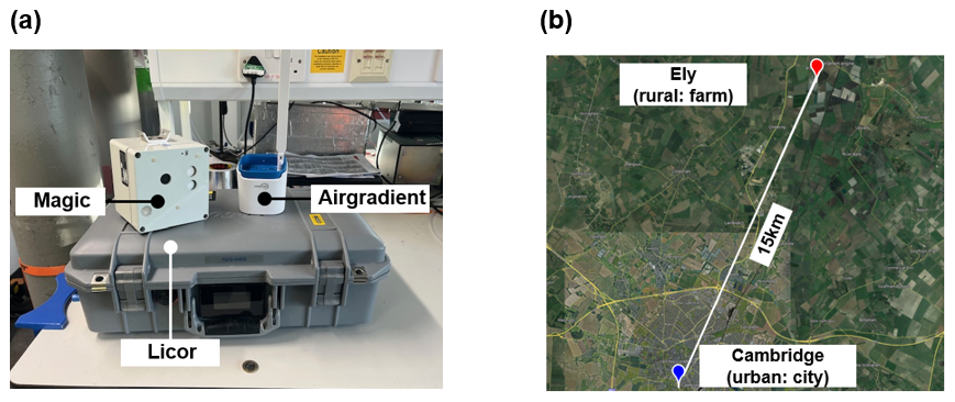
Figure 1 Instrumentation and study sites. (a) LC CO₂ devices (Magic and AirGradient nodes) and the reference LI-COR CO₂ analyser. (b) Map showing the locations of the rural and urban study sites. Background imagery in (b) from Google Earth Pro (Imagery © 2026 Google; map data © 2026 Google).

2.2 Meteorological data and statistical analysis

The performance of the LC data was assessed against the reference measurements using a range of statistical indicators, including root mean square error (RMSE), mean absolute error (MAE), coefficient of determination (R²), and the slope and intercept of a least-squares linear regression fit. Overall results were consolidated using a Taylor diagram, a two-dimensional statistical visualisation that combines three key metrics: standard deviation (SD), Pearson's correlation coefficient (r), and centred root mean square error (cRMSE), which corresponds to the RMSE of bias-corrected data. This was implemented using the openair package in R (Carslaw and Ropkins, 2012).

Supporting meteorological data for London Heathrow airport, 51°28^′39.0^′′ N 0°27^′41.0^′′ W which is approximately 100 km from the rural site and Lakenheath airport, 52°25^′12.0^′′ N 0°34^′00.0^′′ E approximately 25 km from the rural location, were obtained from the National Oceanic and Atmospheric Administration (NOAA) Integrated Surface Database (ISD) using the R worldmet package (Carslaw, 2020).

2.3 Low-Cost CO₂ Sensor Nodes and reference instrument

A bespoke portable monitoring system, known as the “Magic Box”, was initially utilised for CO₂ and air quality measurements at both study locations. This device has been successfully used in previous air quality studies in urban environments (Song et al., 2018). CO₂ was monitored using the original equipment manufacturer (OEM) device Senseair K33 sensor (Senseair, 2025a), which operates on NDIR technology. The Automatic Baseline Correction (ABC) default setting in the K33 had been turned off, thus limiting error associated with ABC (Sect. 2.4.1). A pair of the Magic boxes was collocated outdoors with a reference CO₂ monitor for a period of 12 d at the urban site (7 to 18 December 2022). The nodes were then deployed at the rural site between 20 December and 22 January 2023 (∼ 1 month) in close proximity to a rural reference monitor (< 200 m). The out-of-the-box CO₂ data were corrected to the reference data obtained from the reference LI-COR CO₂ instrument using a 2 d period (14–15 December 2022) during the 12 d initial collocation at the urban site.

The results (see Sect. 3.5) from those initial deployments informed the decision to incorporate an additional portable CO₂ monitoring sensor system, the AirGradient Open Air outdoor air quality monitor. This device measures particulate matter (PM), total volatile organic compounds (TVOCs), CO₂, temperature, and relative humidity. The selection of this alternative LC device was motivated by the improved design of its weatherproof housing, which incorporates mesh openings that allow enhanced air exchange relative to the Magic box. This design reduces the likelihood of air stagnation within the enclosure and minimises internal humidity variability in response to changes in external environmental conditions. CO₂ mixing ratios were specifically measured using the Senseair S8 NDIR sensor (Senseair, 2025b). Unlike the Magic devices, the ABC setting in the AirGradient with the S8 sensor was active by default when the AirGradient units were sourced. We also assessed the viability of Senseair Sunrise sensors for rural application using a version of AirGradient that incorporated Sunrise CO₂ sensor (with the ABC off) as the main CO₂ detector. To evaluate the network applicability of LC CO₂ in rural settings, we deployed a network (four nodes) made up of slightly modified AirGradient Open Air outdoor that used Senseair Sunrise CO₂ OEM device (Senseair, 2025c). This modification to the CO₂ detector in the AirGradient was informed by the need to reduce power demand in the sensor system, as the S8 average current is orders of magnitude higher than Sunrise (18 A compared to 1–34 µA). Although the CO₂ detectors used in the LC devices in this study were all sourced from the same manufacturer, the analytical approach and recommendations for improved performance are generalisable and can be applied to other NDIR or LC CO₂ sensors.

For the purposes of this study, we focus exclusively on CO₂ measurements from these sensor deployments, and not on the other measured parameters by the same sensor platforms. We used LI-COR LI-7815 CO₂/H₂O instrument co-located in the same environment as our reference grade analyser. It is based on an Optical Feedback-Cavity Enhanced Absorption Spectroscopy (OF-CEAS), with a 100 ppb resolution at 1 s averaging and response time less than 2 s (LI-COR, 2025). Span and zero calibrations of the reference analysers were performed at the beginning of each deployment using certified 400 ppm CO₂ in N₂ and synthetic air (< 1 ppm CO₂), respectively. The calibration gas standards were supplied by BOC Ltd and were traceable to national standards. The reference data were averaged to 5 min resolution to match the sampling rate of the AirGradient LC CO₂ used in this study. Figure 1a shows an image of the different instrumentation and Table 1 summarises the information for the various sensor platforms, deployment types and duration of monitoring for our study.

Table 1 Summary of the sensor system, CO₂ type and configuration, form, number of devices and duration of deployment of study.

Scale corrections for the LC AG S8 devices were derived from collocation measurements conducted at rural and urban sites between 1 and 18 August 2023. The resulting correction parameters were applied throughout the deployment period. A similar approach was adopted for the LC AG Sunrise devices within the network, using laboratory collocation measurements from all four devices conducted between 12 and 20 June 2024.

2.4 Sources of errors in LC NDIR CO₂

2.4.1 Effect of OEM Automatic Baseline Correction (ABC) on CO₂ signal

Automatic Baseline Correction (ABC) is a CO₂ signal processing feature available as part of the NDIR CO₂ sensors employed in this study. Initially, the sensor manufacturer recommended enabling this function, as it is intended to correct for baseline drift over time. The ABC algorithm is activated when the measured CO₂ baseline falls below the background mixing ratio, typically set by default at 400 ppm. The system periodically assesses whether this condition has been met over a predefined interval, usually 10 d, although this period may vary. If the sensor records CO₂ mixing ratios below 400 ppm for the majority of that interval, the algorithm calculates the deviation and applies an automatic correction to the baseline.

ABC step-change correction

Step correction was required only for the rural AirGradient (AG) LC device. No evidence of step changes was observed in the AG S8 deployed at the urban site, nor was step correction required for the Magic K33 or AirGradient Sunrise devices, both of which had automatic baseline correction (ABC) deactivated (Table 1).

As major step changes occurred infrequently in the LC AirGradient S8 sensors used in this study, they were identified through manual inspection of scatter plots of the co-located measurements. Periods during which the ABC was triggered were identified by examining the co-location data in short batches (approximately 2 weeks) against measurements from the reference instruments. A batch was considered indicative of an ABC trigger when the coefficient of determination (R²) was low (< 0.6) and two distinct clusters were evident in the scatter plot (Fig. 2b). The associated step change was then identified as an abrupt shift in the measured CO₂ mixing ratio (around 11:00 UTC on 13 August, Fig. 2a). For each step change, its position in the time series and magnitude were determined. The magnitude was estimated as the difference between the CO₂ mixing ratio at the occurrence of the step and the subsequent CO₂ measurement. Two corresponding lists were then constructed: the positions of the identified steps (posco2i) and their respective magnitudes (stepco2i).

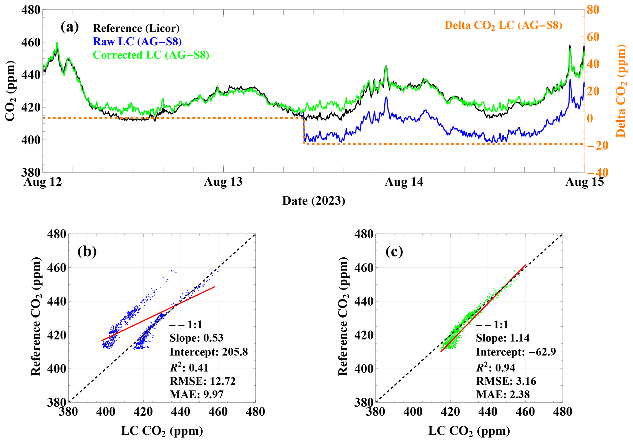
Figure 2 Comparison of LC AirGradient S8 CO₂ measurements with the reference instrument, illustrating the effect of step correction. (a) Time series showing the identified step changes and their magnitudes; (b) uncorrected LC CO₂ measurements against the reference measurements; and (c) step-corrected LC CO₂ measurements (following correction for the ABC step) against the reference measurements.

To illustrate the correction procedure, consider a list of raw CO₂ records. Suppose that step changes are identified at positions posco2i = {100, 121, 335},

with corresponding magnitudes

stepco2i = {10, −13, 8} ppm.

A cumulative offset is calculated to account for the persistence of each step change. The correction is implemented as follows:

1. A δ CO₂ array of length is initialised with zeros.

2. An offset of 0 ppm is assigned to observations 1–99.

3. Following the first step, an offset of +10 ppm is assigned to observations 100–120.

4. Following the second step, the cumulative offset becomes −3 ppm (+10–13) and is assigned to observations 121–334.

5. Following the third step, the cumulative offset becomes +5 ppm (+10−13+8) and is applied from observation 335 to the end of the record.

The resulting δ CO₂ time series is subtracted from the raw CO₂ measurements to obtain the step-corrected CO₂ mixing ratios. Thus, rather than correcting each step independently, the procedure accounts for the cumulative effect of successive changes in the instrument baseline.

Step changes were observed only to a limited extent and occurred in one device (AirGradient LC-S8) deployed at the rural site. Figure 2 shows an example of the step-correction procedure for this instrument.

Baseline drift correction

Whilst we did not observe baseline drift in our study when the ABC was deactivated, long-term drift is expected to introduce error into the measurements. Users should therefore characterise this drift by detrending the data prior to applying the environmental correction framework presented in this work (Sect. 3.3).

For devices deployed as part of a network, users can correct for baseline drift using the approach described by Müller et al. (2020). This method exploits periods of minimal horizontal CO₂ gradients and a well-mixed boundary layer to derive time-dependent offset corrections relative to the nearest reference CO₂ measurement within the network. In the absence of a reference instrument, a modified version of this approach can be used, whereby an LC NDIR device is deployed away from local emission sources and at an elevated location (> 20 m), with the remaining network devices referenced to this sensor. Any gradual intrinsic drift in the reference LC device can then be corrected by comparing monthly mean CO₂ mixing ratios with hemispheric background CO₂ measurements (from Mauna Loa for the Northern Hemisphere and American Samoa for the Southern Hemisphere) over the corresponding study period (Pétron et al., 2026).

2.4.2 Effect of external environmental factors on LC CO₂ signal

Previous studies have demonstrated that LC used for the measurement of other atmospheric species are influenced by environmental parameters, particularly temperature (Crilley et al., 2018; Di Antonio et al., 2018; Mead et al., 2013; Spinelle et al., 2017). These effects are often attributable to inherent trade-offs between portability and cost on the one hand, and instrument sensitivity and measurement resolution on the other. Another factor that suggests the possible effect of external environmental parameters on the performance of LC under real world application is the fact that they are often calibrated under controlled environmental conditions in the lab. NDIR is a spectroscopic technique, and any external factors that might affect its optics and detectors will impact sensor performance. The extreme temperature diurnal variabilities characteristic of summertime might affect the optics and invariably sensor performance. On an extended timescale, we postulate that pressure could additionally affect the performance of the CO₂ sensor. The provenance of this effect can be related to the fact that the sensors OEM are calibrated at a fixed pressure and report the signal in mixing ratios (parts per million, ppm).

Previous studies have demonstrated that variations in pressure can affect the observed mixing ratios if not adequately accounted for (Müller et al., 2020; Gaynullin et al., 2023). In addition, pressure-induced spectral broadening can affect the accuracy of LC NDIR devices. However, this effect is generally smaller than that associated with pressure-dependent changes in number density. For most applications, correcting for the latter is therefore considered sufficient (Gaynullin et al., 2023).

Pressure correction methodology

In the absence of a controlled laboratory experiment similar to that reported by Gaynullin et al. (2023), we leveraged the co-location measurements to derive corrections for the effects of two major environmental factors, pressure and temperature, on the LC NDIR CO₂ measurements. The LC AG-S8 device deployed at the urban site was used to derive the pressure-correction parameters. To minimise the confounding influence of high temperatures on the LC CO₂ response, only measurements from the winter period (15 January–15 February 2025) were used to develop the pressure-correction algorithm.

The ratio of the offset-corrected LC CO₂ measurement to the reference CO₂ measurement was calculated and related to the normalised pressure, $P/P_{\mathrm{0}}$ where P₀= 1012 mbar and P uses the hourly pressure data described in Sect. 2.2. The CO₂ offset was determined from the mean difference between a subset of the LC AG-S8 and reference measurements obtained under conditions close to the selected standard conditions (pressure = 1012 ± 2 mbar and temperature = 20 ± 1 °C). For applications where co-located reference measurements are unavailable, an approximate offset may instead be estimated, where a significant factory bias is evident, from the difference between the lowest observed raw LC NDIR CO₂ value and the Northern Hemisphere background CO₂ mixing ratios during the corresponding study period (Pétron et al., 2026).

A linear relationship was observed between the LC-to-reference CO₂ ratio and $P/P_{\mathrm{0}}$, with the regression describing the pressure-dependent correction factor. Figure 3a shows the relationship between the LC $/$ reference CO₂ ratio, $P/P_{\mathrm{0}}$, and ambient temperature. The fitted expression (slope and intercept in Fig. 3a) is analogous to the compensation coefficient described by Gaynullin et al. (2023). The pressure-corrected CO₂ mixing ratios, ${\mathit{\chi }}_{{\mathrm{CO}}_{\mathrm{2}}}^{\text{reference}}$ is therefore defined as

$$\begin{array}{}\text{(1)}& {\mathit{\chi }}_{{\mathrm{CO}}_{\mathrm{2}}}^{\text{reference}}=\left({\displaystyle \frac{{\mathit{\chi }}_{{\mathrm{CO}}_{\mathrm{2}}}^{\text{offsetcorr}}}{K}}\right)+\text{offset}\left(\text{at}{P}_{\mathrm{0}}\right)\end{array}$$

where

$$\begin{array}{}\text{(2)}& K=\mathrm{1.05}\cdot \left({\displaystyle \frac{P}{P_{\mathrm{0}}}}\right)-\mathrm{0.08}\end{array}$$

and offset  (at  P₀) is expected to be zero for an ideal calibrated device, in the case of the device used in this study,

$$\text{offset}\left(\text{at}{P}_{\mathrm{0}}\right)=-\mathrm{0.02}-\mathrm{0.031}\cdot {\mathit{\chi }}_{{\mathrm{CO}}_{\mathrm{2}}}^{\mathrm{offsetcorr}},$$

with P₀= 1012 mbar (Fig. S5 in the Supplement).

The offset (at P₀) is obtained by fitting a linear model to the difference between ${\mathit{\chi }}_{{\mathrm{CO}}_{\mathrm{2}}}^{\text{reference}}$ and $\left(\frac{{\mathit{\chi }}_{{\mathrm{CO}}_{\mathrm{2}}}^{\text{offsetcorr}}}{K}\right)$ at $P=P_{\mathrm{0}}=$ 1012 mbar where K= 0.97 for a range of ${\mathit{\chi }}_{{\mathrm{CO}}_{\mathrm{2}}}^{\text{offsetcorr}}$ spanning low to high mixing ratios. The correction is formulated such that, at the ambient pressure (P=P₀), the pressure-corrected LC measurement approaches the reference CO₂ measurement i.e., ${\mathit{\chi }}_{{\mathrm{CO}}_{\mathrm{2}}}^{\text{Pcorr}}={\mathit{\chi }}_{{\mathrm{CO}}_{\mathrm{2}}}^{\text{reference}}$. An optimised version of Eqs. (1) and (2) was used to generate the pressure corrected CO₂ mixing ratios as formulated in Eq. (3).

$$\begin{array}{}\text{(3)}& \begin{array}{rl}{\mathit{\chi }}_{{\mathrm{CO}}_{\mathrm{2}}}^{\text{Pcorr}}& =\left[{\displaystyle \frac{\mathrm{1}}{\left(\mathrm{1.05}\cdot \left(\frac{P}{P_{\mathrm{0}}}\right)-\mathrm{0.08}\right)}}\cdot {\mathit{\chi }}_{{\mathrm{CO}}_{\mathrm{2}}}^{\text{offsetcorr}}\right]\\ & +\left(-\mathrm{0.02}-\mathrm{0.031}\cdot {\mathit{\chi }}_{{\mathrm{CO}}_{\mathrm{2}}}^{\text{offsetcorr}}\right)\end{array}\end{array}$$

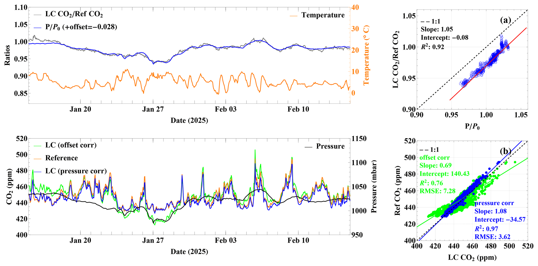
Figure 3 Pressure effect and correction for the LC AG-S8 CO₂ sensors. (a) Pressure dependence, expressed as $P/P_{\mathrm{0}}$ and ${\mathit{\chi }}_{{\mathrm{CO}}_{\mathrm{2}}}^{\mathrm{LC}}/{\mathit{\chi }}_{{\mathrm{CO}}_{\mathrm{2}}}^{\mathrm{ref}}$, at the urban site (15 January–14 February 2025). (b) Uncorrected and pressure-corrected sensor data compared with the reference.

Figure 3b shows the comparison of the input CO₂ and pressure-corrected CO₂. As the temperature remained relatively low (< 10 °C), with limited diurnal variability, pressure was identified as the environmental parameter most strongly associated with the observed the LC $/$ reference CO₂ ratio variability, as indicated by the strong correlation in Fig. 3a. The correction approach yields a compensation expression that depends on both pressure and CO₂ mixing ratios, as it is derived empirically from real-world measurements in which the CO₂ mixing ratio varies with pressure. Applying the pressure correction substantially improved the agreement, with R² increasing from 0.69 to 0.97 and the RMSE decreasing from 7.3 to 3.6 ppm, Fig. 3b. Analysis of the residual dependence of the uncorrected CO₂ reading with the pressure for the analysis shows the error associated to be approximately 0.5 ppm mbar⁻¹ about five times that reported by Müller et al., 2020.

Temperature correction methodology

Two sets of correction parameters were derived for the two variants of the low-cost (LC) AirGradient CO₂ sensor used in this study: the AG-S8 and AG-Sunrise.

For the long-term co-location deployments at the rural and urban sites, measurements from the urban co-location were used to derive a generic temperature correction, which was subsequently applied to the LC AG-S8 devices at both locations. To minimise overfitting whilst adequately representing the two temperature extremes, subsets of the summer (17–24 August 2023) and winter (29 November–6 December 2023) measurements from the urban co-location site were used to derive the temperature correction.

The first step involved calculating the ratio of the pressure-corrected LC CO₂ measurement to the corresponding reference CO₂ measurement and examining its dependence on the absolute sensor temperature (K). Figure 4a–b shows that the relationship between these variables is non-linear. A power-exponential function provided the best representation of the temperature dependence of the CO₂ sensor sensitivity, resulting in the correction described by Eq. (4):

$$\begin{array}{}\text{(4)}& {\displaystyle \frac{{\mathit{\chi }}_{{\mathrm{CO}}_{\mathrm{2}}}^{\text{Pcorr}}}{{\mathit{\chi }}_{{\mathrm{CO}}_{\mathrm{2}}}^{\text{Tcorr}}}}=\left[A_{\mathrm{S}\mathrm{8}}+\left(B_{\mathrm{S}\mathrm{8}}\cdot {C_{\mathrm{S}\mathrm{8}}}^{\text{sensorT}}\right)\right]\end{array}$$

Here, ${\mathit{\chi }}_{{\mathrm{CO}}_{\mathrm{2}}}^{\text{Pcorr}}$ and ${\mathit{\chi }}_{{\mathrm{CO}}_{\mathrm{2}}}^{\text{Tcorr}}$ represent the pressure-corrected and temperature-corrected CO₂ mixing ratios, respectively, and sensorT is the sensor temperature expressed in kelvin. The optimal fit parameters for the LC AG-S8 sensor used in this study were A_S8= 0.95, B_S8= 4.40 × 10⁻⁵ and C_S8= 1.03 (Fig. 4c).

The LC AG-Sunrise nodes used in the network deployment were corrected using the same functional form given in Eq. (4), with parameters derived specifically for this sensor variant. The temperature-correction results for the four nodes during their laboratory co-location (12–20 June 2024) are presented in Fig. S6 and Table S1 in the Supplement. The daytime temperature-dependent biases observed in the LC AG-Sunrise measurements, which were particularly evident between 18 and 20 June 2024 (Fig. S6a), were substantially reduced after accounting for the temperature dependence (Fig. S6b). Across the four nodes, the RMSE decreased from approximately 7.5–12 ppm for the pressure-corrected measurements to 2.7–3.9 ppm following combined pressure and temperature correction (Fig. S6c).

The approximately 10 ppm bias evident during the warmer summer period was largely removed following temperature correction (Fig. 4d). Consequently, the RMSE decreased from 7.3 ppm for the pressure-corrected measurements to 2.2 ppm following combined pressure and temperature correction (Fig. 4e). Based on this analysis, the magnitude of the temperature effect, estimated from the residual difference between the pressure-corrected and pressure-temperature-corrected data, was 0.6 ppm K⁻¹.

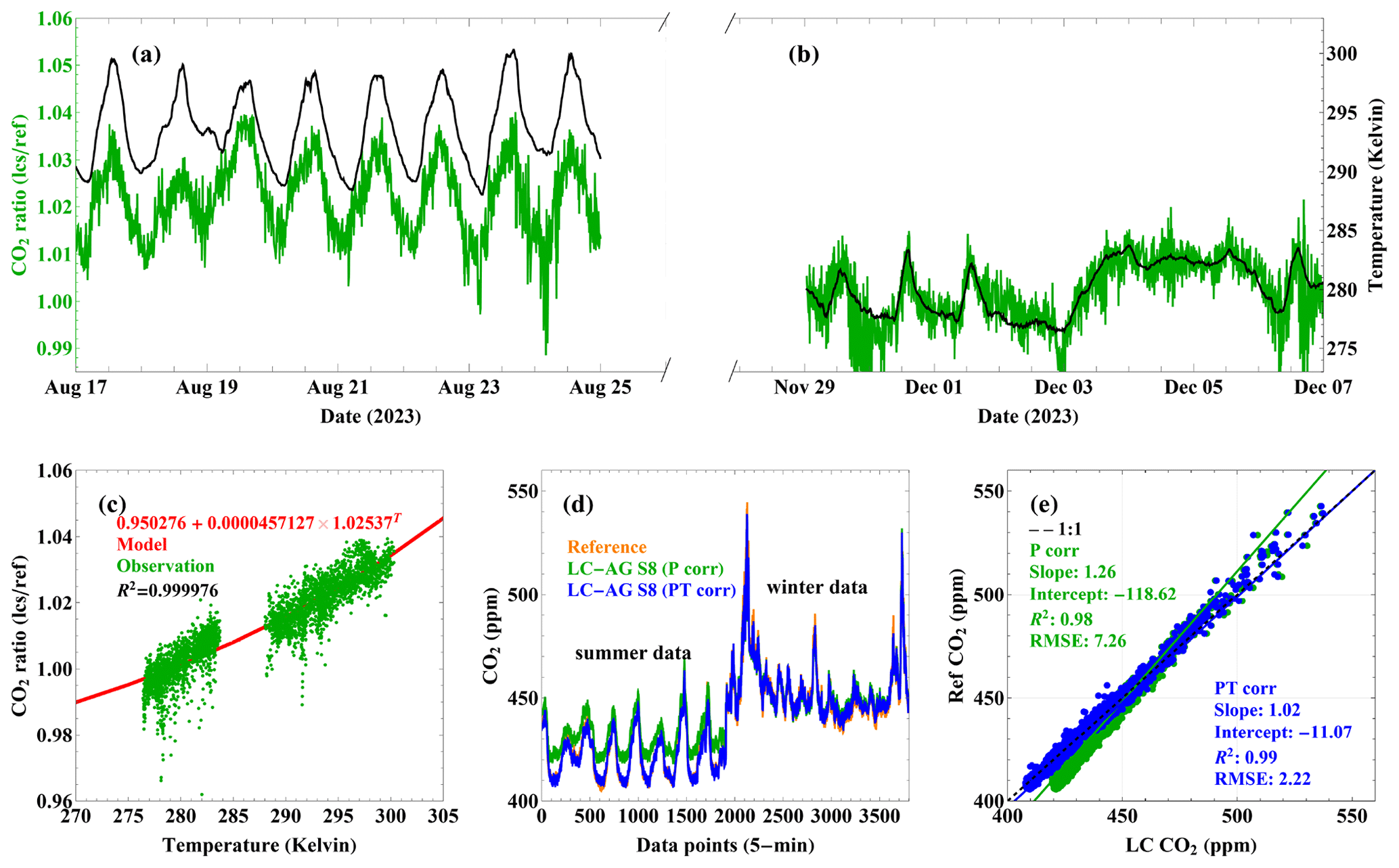
Figure 4 Temperature effect and correction for LC AirGradient S8 CO₂ sensors. (a–b) CO₂ ratio ($X_{\mathrm{sensor}}/X_{\mathrm{ref}}$) and temperature during selected summer (17–24 August 2023) and winter (29 November–6 December 2023) periods at the urban site, (c) observed versus modelled temperature dependence, (d) pressure- and temperature-corrected CO₂ relative to the reference, and (e) scatter plot of the data in (d).

2.4.3 Effect of elevated RH on LC CO₂ signal

An NDIR sensor measures CO₂ mixing ratios by comparing two infrared (IR) signals from the same IR source at two distinct wavelengths (IR-high and IR-low), detected using a dual-bandpass filter after transmission through the air sample within an optical cavity. For CO₂ measurements, the IR-high channel is centred at approximately 3.9–4.0 µm, where CO₂ exhibits negligible absorption (reference band), while the IR-low channel is centred around 4.26 µm, corresponding to a strong CO₂ absorption band. In the presence of CO₂, the IR-low signal is attenuated, resulting in a reduced signal magnitude relative to the IR-high channel.

The presence of water vapour can influence the IR-low channel, as H₂O exhibits weak but non-zero absorption within the 3–5 µm region, potentially leading to an overestimation of CO₂ mixing ratios in NDIR measurements. Under conditions of extremely high relative humidity, condensation may occur on the optical cavity mirrors, causing additional signal attenuation and resulting in spurious CO₂ readings. The effect of RH and water condensation on the performance of NDIR is a well-known phenomenon (Cai et al., 2025; Martin et al., 2017; Pereira and Ramos, 2022; Ren et al., 2025; Wu et al., 2023; Xu et al., 2024). Most LC devices have the CO₂ sensing unit housed in a weatherproof unit and tend to rely on passive sampling to minimise power demand. In the absence of an internal heating system that helps reduce water condensation, in combination with a preference for passive sampling in LC (to reduce power demand), there is an increased likelihood that high RH episodes would affect the CO₂ measurement. Such environmental conditions are more common in rural applications than in urban settings, where average temperatures are relatively higher (Si et al., 2024; Weng et al., 2004). We investigated the effect of RH by deploying the same pair of Magic boxes initially in the urban (December 2022) and subsequently in the rural environment (January 2023).

2.5 Framework for LC CO₂ data processing

Based on the known sources of errors discussed in Sect. 2.4, and the results presented in Sect. 3.1–3.2, the following data correction protocol (Fig. 5) is proposed.

Figure 5 Framework for correction of LC CO₂ signal.

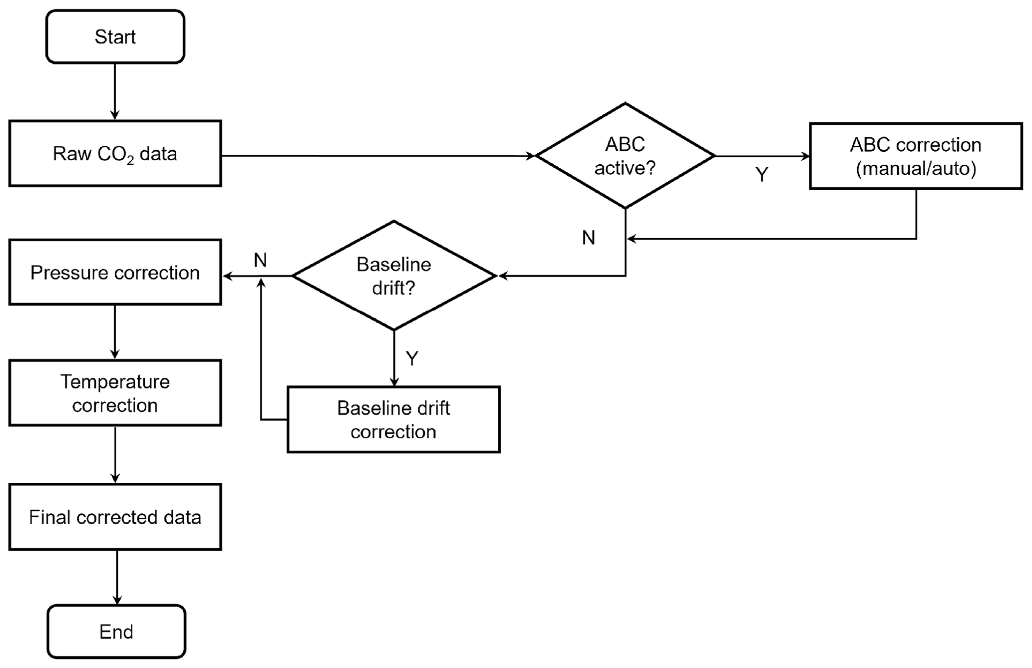
This framework presents a logical approach for improving the precision and accuracy of LC CO₂ for atmospheric application. We applied this data correction framework to evaluate the suitability of a network of CO₂ sensors in rural applications.

3 Results and Discussion

3.1 CO₂ correction for ABC

While not all nodes exhibited a significant ABC correction, instances where this occurred were clearly distinguishable as systematic errors, as illustrated in Fig. 2. As expected, a significant improvement in agreement between the LC and the reference instrument was observed when this correction was implemented (RMSE = 3.2 ppm, R²= 0.94 compared to 12.7 ppm, R²= 0.41). Although this seems to suggest the only correction required is a simple ABC correction, it is worth noting that the data shown is for only a short period where the effects of environmental factors might be minimal if the meteorological conditions are ideal (minimal impact of temperature and pressure). For long-term (months) application, we evaluated the effects of environmental factors, as discussed in the next section.

While there is merit to using the ABC method to correct potential drifts in CO₂ readings below true hemispheric background level, the method has limitations. A temporary decrease in CO₂ mixing ratio may result from environmental factors rather than true sensor drift, as will be discussed in the following section. Consequently, the automatic correction may introduce errors into the actual CO₂ measurements.

3.2 Physical correction for the effect of environmental factors

We primarily present the results of the physical correction applied to one of the LC AirGradient S8 sensors deployed for an extended period of 19 months, from May 2023 to February 2025, at the urban study site (Fig. 6). Equivalent results for the rural site are presented in Fig. S1. To assess the performance of the correction protocol, we also present results obtained using simple linear scaling, a method commonly used to calibrate out-of-the-box sensor measurements (Fig. 6b).

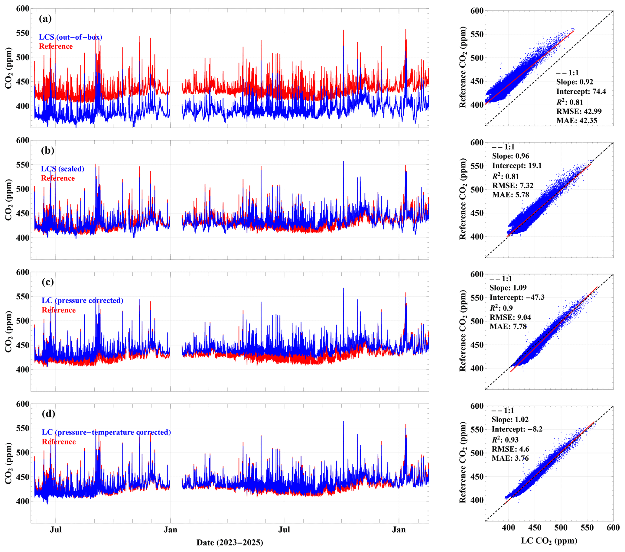
Figure 6 Results of different calibration stages for the LC Airgradient-S8 CO₂ signal for the period 22 May 2023 to 18 February 2025 at the urban location. (a) Factory calibration, (b) simple linear calibration using a fixed period (1–18 August 2023), (c) pressure only correction of the out-of-box signal and (d) pressure and temperature correction of out-of-box signal.

Linear scaling substantially improved agreement between the LC AirGradient S8 and the reference instrument during the co-location period, reducing the RMSE from 43 ppm for the out-of-the-box measurements to 7.3 ppm for the scaled data. A similar improvement was observed in the MAE), which decreased from 42 to 5.8 ppm, while the R² remained unchanged at 0.81. The invariance of R² is expected because linear scaling does not alter the strength of the linear relationship between the two datasets (Fig. 6a and b). This differs from corrections that account for the effects of environmental parameters, such as temperature and pressure (Fig. 6d and c). Correcting the CO₂ measurements for pressure effects improved R² to 0.90, with an RMSE of 9.1 ppm (Fig. 6c). Further improvement was achieved by applying the combined pressure and temperature correction, which resulted in an R² of 0.93 and an RMSE of 4.6 ppm (Fig. 6d).

Improved long-term performance was also observed for the LC AirGradient sensor deployed at the rural site (Fig. S1). The RMSE decreased from 19 ppm for the out-of-the-box measurements to 14.3, 13.6 and 10 ppm for the scaled, pressure-corrected and combined pressure-temperature corrected data, respectively. Correspondingly, R² increased from 0.92 for both the out-of-the-box and linearly scaled data to 0.94 and 0.95 following the pressure and combined pressure-temperature corrections, respectively.

Figures 7 and 8 present results for LC AG S8 over a shorter period, helping to highlight the effects of pressure/temperature and how the correction improves the CO₂ performance relative to the reference.

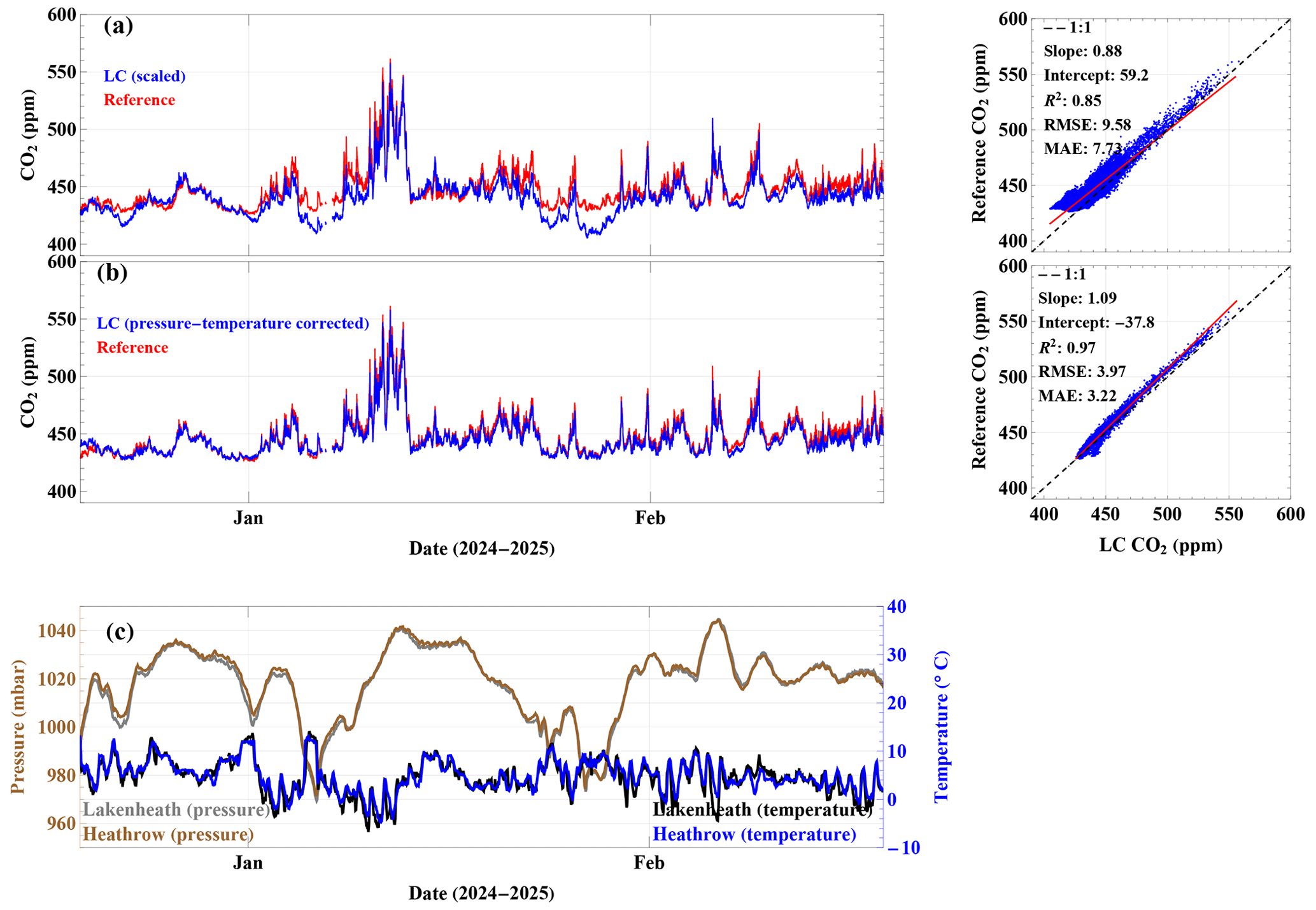
Figure 7 Comparison of two correction methodologies for the LC Airgradient S8 for the period 19 December 2024 to 18 February 2025 at the urban location. (a) simple linear scaling correction, (b) combined pressure-temperature corrected raw signal, (c) hourly pressure and temperature observation from London Heathrow and Lakenheath airport.

The results in Fig. 7 shows an example of a 2-month period in winter when temperature effects (mean ± SD = 4.9 ± 3.27 °C) are minimal, and the diurnal variability is small, but the pressure change is significant (pressure range 970–1045 mbar, average 1018.7 ± 14.70 mbar). The significant dips in the scaled LC AG S8 CO₂ readings relative to the reference before 22 December 2024, around 6 January and between 22 and 30 January 2025 in Fig. 7a coincide with an ambient pressure drop from around 1020 mbar to as low as 960 mbar. The pressure-temperature corrected LC CO₂ tracks the reference data better with improved R² (0.97 vs. 0.85) and RMSE (3.2 vs. 9.6 ppm).

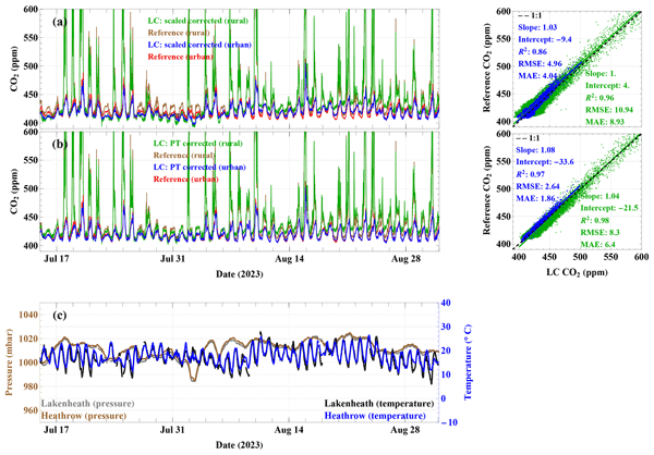
In contrast, Fig. 8 presents an example in summertime when the effect of temperature dominates the error on the LC AG S8 CO₂ performance for both the urban and rural site, and the pressure effect is minimal (1012.0 ± 6.82 mbar). As can be seen in Fig. 8a for the scaled CO₂ correction, the LC signals show daytime overestimation at both the urban and rural sites, which coincides with daytime temperatures well above 10 °C. The effect of pressure is minimal over this period except for 2–3 August, where the scaled LC CO₂ show both daytime and nighttime dips, which is characteristic of pressure drop exemplified previously in Fig. 7.

The pressure-temperature corrected data showed improved agreement, with RMSE and R² values of 2.6 ppm and 0.97 at the urban site and 8.3 ppm and 0.98 at the rural site, respectively, compared with 5 ppm and 0.86 at the urban site and 11 ppm and 0.96 at the rural site for the simple scaling correction.

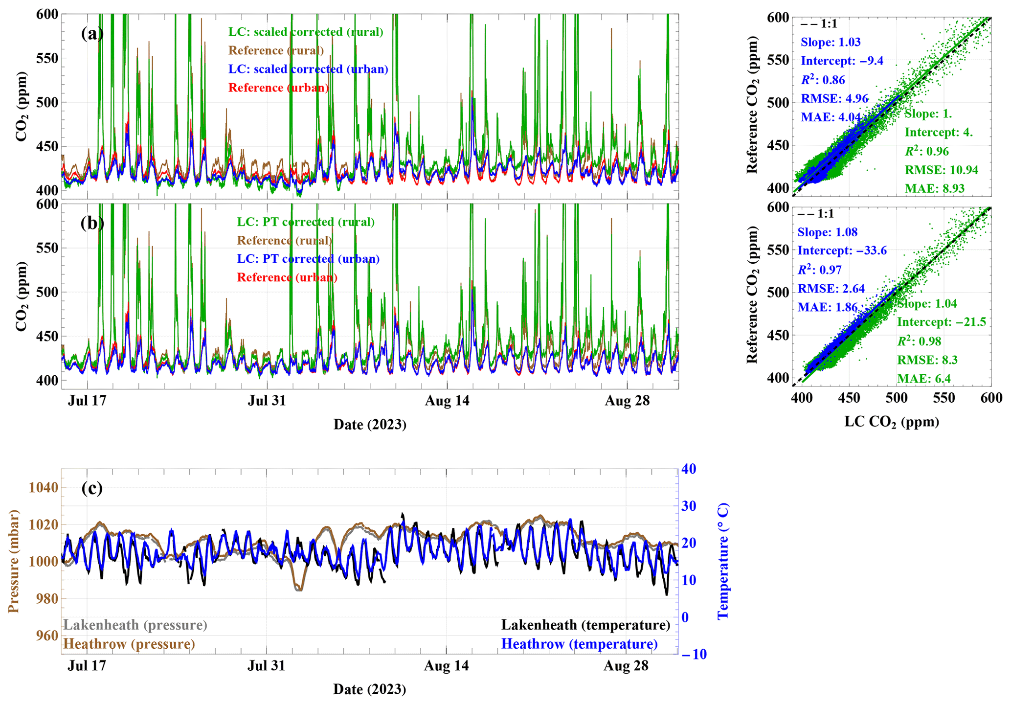
Figure 8 Comparison of two correction methodologies for the LC AirGradient S8 for the period 15 July to 31 August 2023 at the urban and rural locations. (a) simple linear scaling correction, (b) combined pressure-temperature corrected raw signal, (c) hourly pressure and temperature observation from London Heathrow and Lakenheath airport.

3.3 Assessment of the LC CO₂ data processing framework

Following the framework in Sect. 2.5, the performance of each data correction step-including the raw and simply scaled data relative to co-located reference measurements for the urban and rural deployments for the LC AG S8 devices, are summarised using a Taylor diagram (Fig. 9). Data points located closer to the reference indicate better agreement with the reference measurements. Standard deviations are shown as arcs of increasing radius along the x- and y-axes, Pearson correlation coefficients are indicated by grey radial lines extending from the origin (0 on the y-axis to 1 on the x-axis), centred root mean square error (cRMSE) is represented by brown contours of increasing magnitude, referenced to the point on the x-axis. For the full urban dataset (Fig. 9a), simple scaling provides only a marginal improvement in cRMSE relative to the raw data (7.3 ppm compared with 7.2 ppm; indicated by the brown band in Fig. 9), while the correlation remains unchanged (r= 0.9; grey radial scale in Fig. 9). However, the scaling reduces signal variability (SD = 15.6 ppm) compared with the raw data (SD = 16.3 ppm) and the reference measurements (SD = 16.6 ppm; purple marker on the dashed black arc in Fig. 9a). In contrast, the correction approaches introduced in this study result in clear improvements across all three statistics. Both the pressure-corrected and pressure-temperature-corrected datasets show reduced cRMSE (4.3 ppm), improved correlation (r= 0.97), and standard deviations closer to the reference data (SD = 16 ppm). While the pressure correction alone improves both cRMSE and correlation relative to the raw and simply scaled data, the combined pressure-temperature correction provides the closest agreement with the reference measurements. Similarly, the comparative statistics for the rural site for the duration of study showed (Fig. 9b) an slight increase in both r= 0.97 and cRMSE = 11 ppm for the pressure-temperature corrected LC AG S8 compared to the other three dataset (r= 0.96, cRMSE ≈ 13 ppm), there was little change in the SD (∼ 46 ppm) of all dataset due to the large variability observed at the rural site.

Figure S2a and b present results for shorter periods at the urban site in winter and summer, respectively, representing conditions dominated by pressure variability (Fig. S2a) and temperature variability (Fig. S2b) as presented in Sect. 3.2. During the winter period, a substantial improvement is observed between the raw and pressure-corrected data (cRMSE from 7.2 to 3.8 ppm, and r from 0.92 to 0.98), with only marginal additional improvement when temperature correction is included. This is consistent with the limited temperature variability during this period (see Sect. 3.2). In contrast, during the summer period, when temperature variability is greater, the combined pressure-temperature correction (cRMSE = 2.5 ppm, r= 0.98) produces an improvement compared with the pressure-only correction (cRMSE = 3.5 ppm, r= 0.97). The corresponding summer rural deployment is shown in Fig. S2c, with cRMSE values of 11, 9, and 8 ppm and r of 0.98, 0.99, and 0.99 for the scaled, pressure-corrected, and pressure–temperature corrected data, respectively.

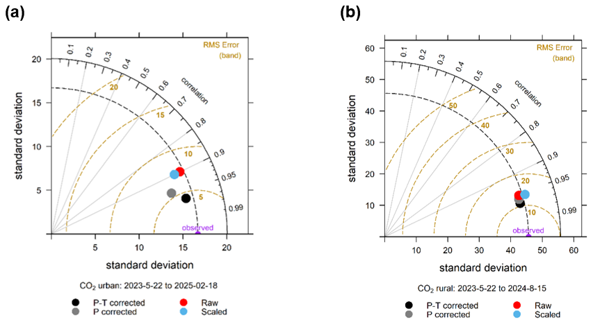
Figure 9 Taylor diagram comparing raw, scaled, pressure corrected, and pressure-temperature corrected CO₂ measurements for the LC Airgradient S8 with co-located reference observations at the (a) urban site for 22 May 2023–18 February 2025 and (b) rural site for 22 May 2023–15 August 2024. Data points located closer to the reference indicate better agreement with the reference measurements.

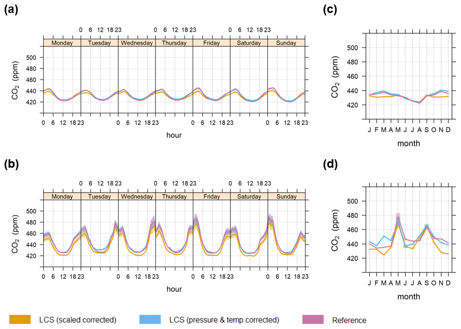
Figure 10 Comparison of rural and urban CO₂ measurements for the LC Airgradient S8 (scaled, pressure-temperature corrected) and reference device for the duration of the study. (a) Day-of-week diurnal profile at the urban site, (b) equivalent profile at the rural site, (c) monthly averages at the urban site, and (d) monthly averages at the rural site.

3.4 Suitability of LC CO₂ in rural applications

3.4.1 Collocation assessment

To assess the potential deployment of LC Airgradient S8 CO₂ monitoring in rural environments, we compared measurements from corrected LC units with those obtained from reference-grade instruments at two locations, as outlined in Sect. 2. Although simple linear scaling produced similar trends to the reference data in both day-of-week diurnal and monthly plots, the LC measurements consistently underestimated CO₂ mixing ratios, particularly during the winter months by approximately 10 and 20 ppm at both urban and rural sites respectively. However, as illustrated in Fig. 10b–d, the LC Airgradient S8 data corrected for pressure and temperature effects from the rural site show very good agreement with the reference measurements, both in terms of absolute values (see statistics in Sect. 3.3) and temporal trends.

Comparison of collocation assessment to other studies

Based on the pressure-corrected measurements, the LC AirGradient S8 and AirGradient Sunrise sensors (Sects. 3.2 and 2.4.2) are capable of measuring ambient CO₂ mixing ratios with an accuracy of approximately 5 ppm. This performance suggests that the sensors can reliably resolve changes in CO₂ mixing ratios exceeding 15 ppm, representing an improvement over the 30 ppm resolution reported by Müller et al. (2020). The performance of the LC AirGradient S8 therefore supports its application in both urban and rural environments, including locations where CO₂ mixing ratios may periodically reach substantially higher values than those typically observed in urban environments.

To facilitate a direct comparison with Gaynullin et al. (2023), we also evaluated the performance of our correction method using the mean absolute percentage error (MAPE) for the LC AirGradient S8 deployments. This metric expresses the measurement error relative to the observed CO₂ mixing ratio. The MAPE ranged from 0.86 % for the urban deployment, where CO₂ mixing ratios were approximately 410–550 ppm, to 1.5 % at the rural site, where CO₂ increased from background levels to approximately 1000 ppm. These errors are lower than those reported by Gaynullin et al. (2023) for their one-dimensional compensation method. However, they are higher than the −0.02 % error reported for the two-dimensional compensation method at 800 ppm, while the lower MAPE obtained for our urban deployment (0.86 %) is comparable to the 0.83 % error reported at a CO₂ mixing ratio of 3000 ppm.

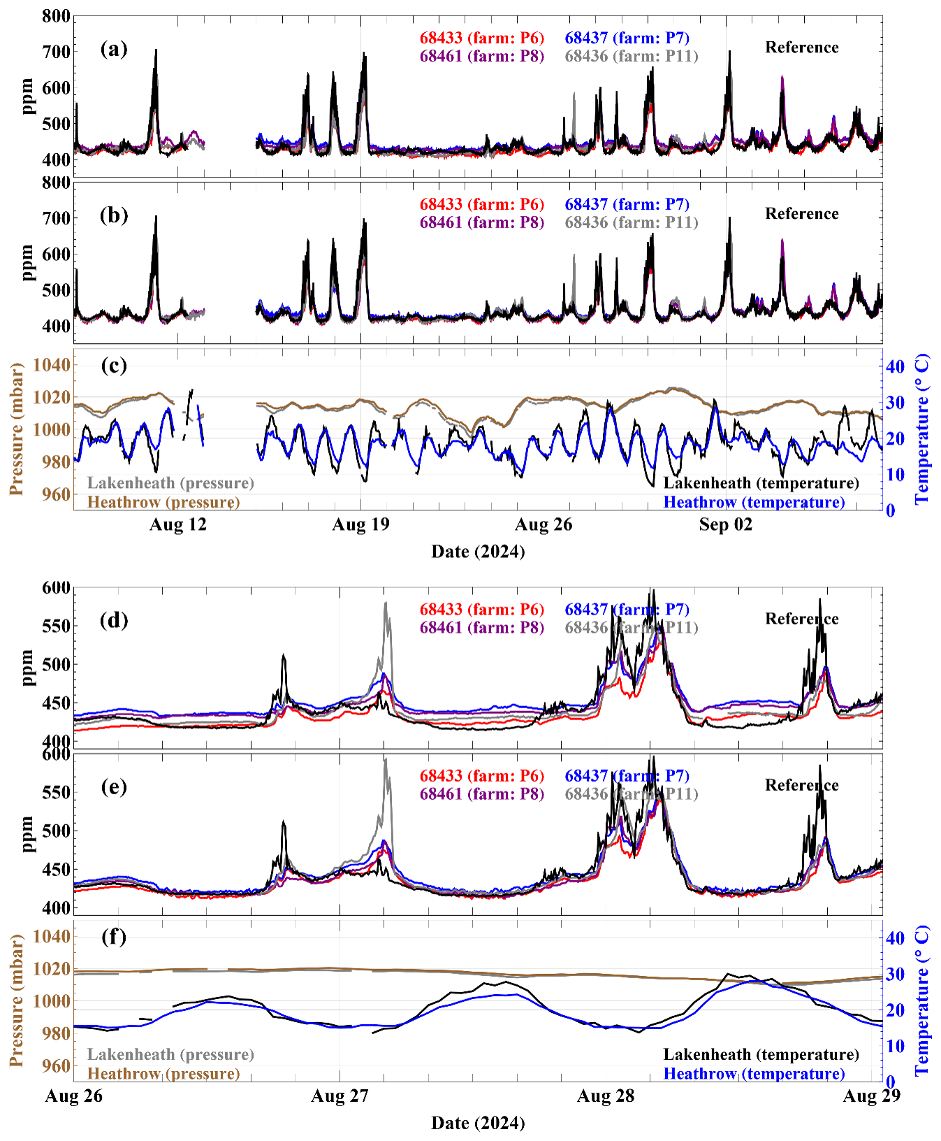
Figure 11 Comparison of two correction methods applied to four LC CO₂ sensors deployed at an arable farm from 8 August to 8 September 2024. Panels (a)–(c) show (a) CO₂ mixing ratios corrected using linear scaling, (b) CO₂ mixing ratios corrected for pressure and temperature, and (c) hourly surface pressure alongside observations from London Heathrow and Lakenheath airports. Panels (d)–(f) show enlarged views of (a)–(c), respectively, for 26–28 August. Missing data at the start of the deployment resulted from cellular transmission issues within the LC network.

3.4.2 Network assessment

A direct statistical comparison with the reference measurements was not performed because the reference instrument was not collocated with any of the sensors within the network (Fig. S7). However, because the reference instrument was deployed within the same land-use environment and at a distance of less than 1 km from each sensor, the slowly varying background CO₂ signal is expected to influence both the LC network and the reference instrument in a similar manner. Deviations from this background signal observed by individual devices can therefore be attributed primarily to local sources and sinks in the immediate vicinity of each measurement location. This rural deployment consequently provides a valuable opportunity to assess the performance of LC devices under rural environmental conditions.

The observed CO₂ mixing ratios were strongly influenced by local emissions associated with crop respiration, particularly during the night, when photosynthesis ceased and the planetary boundary layer was shallower (with above background CO₂ ranging periodically in excess of 200 ppm for a 5 min averaged data). Notably, daytime errors of approximately 15–30 ppm (27–28 August 2024), present in the uncorrected dataset (Fig. 11a and d) were substantially reduced by applying the pressure-temperature correction approach, as demonstrated in the comparison with the reference measurement (Fig. 11b and e). In this case, the correction was primarily driven by temperature, which exhibited marked diurnal variability (Fig. 11c and f), whereas pressure changes over the one-month deployment period were comparatively minor (Fig. 11c). Figure 11e shows that the corrected measurements exhibit a background level comparable to that of the reference data, with intermittent departures from this background. These departures, observed as short-duration enhancements (for example the enhancement of approximately 180 ppm observed at P11 shortly after midnight on 27 August 2024, shown in Fig. 11e), indicate a stronger influence from nearby emission sources (respiration from the crop) at this location compared with other sites within the network.

3.5 Additional artefacts that affect performance of LC NDIR CO₂

Despite all the issues discussed related to environmental effect and baseline correction, poorly designed devices that utilise NDIR CO₂ sensors can still suffer from unintended artefacts related to poor air circulation that presents itself as environmental effect when there is no active sampling. Figure S4 (e and g) shows that there was good agreement between the calibrated LC CO₂ from the Magic K33 devices and the reference instrument (RMSE = 5–7 ppm) during the deployment in the urban location, where the internal RH reading was below 80 % (Fig. S4c). Apart from small daytime differences of approximately 5 °C observed at the urban site, the internal temperature was comparable to the ambient reference temperature during this period (Fig. S4a). In contrast, the lower relative humidity measured inside the LC Magic boxes indicates substantially drier conditions relative to the ambient environment.

In contrast, the results from the calibrated Magic devices (Fig. S4f and h) in the rural environment were very poor (RMSE = 35–61 ppm), as the units only tracked the reference in the first 3–4 d. The internal RH for Magic K33 devices over these periods were generally above 80 % (Fig. S4b). This effect cannot be corrected empirically, as it is inherently non-systematic, unlike the temperature and pressure effects described earlier. It may, however, be mitigated by ensuring adequate air recirculation – such as operating the instrument within a suitably ventilated enclosure-to prevent internal moisture accumulation under colder conditions, or by heating the sampled air where low-power operation is not a constraint.

4 Conclusions

Ambient CO₂ mixing ratios can be effectively monitored using LC when environmental influences, particularly temperature and pressure, are appropriately accounted for. In our study, pressure effects were found to dominate measurement errors under colder conditions and over longer timescales associated with macro-level pressure variations. By contrast, temperature effects were more pronounced in spring and summer, varying on shorter diurnal timescales.

A notable source of measurement uncertainty in CO₂ sensors is the ABC implemented by manufacturers to adjust for sensor drift. This correction often introduces step changes in readings, thereby reducing both precision and accuracy (RMSE = 20 ppm compared to 5 ppm when this is accounted for in our study). To ensure robust data processing, we recommend either disabling the ABC functionality or, where ABC remains active, correcting for any erroneous step changes using the approach described in this study prior to data analysis.

Episodes of extremely high RH can adversely affect the performance of NDIR CO₂ sensors, particularly when sensor housings are poorly ventilated, as observed for the Magic Sunrise CO₂ devices. This can result in anomalously high CO₂ measurements, especially at remote rural sites where high-RH conditions are more prevalent. In contrast, well-ventilated designs, such as the LC Airgradient S8 and Airgradient Sunrise CO₂ devices, demonstrate that NDIR sensors can reliably capture the large temporal variability in CO₂ mixing ratios characteristic of rural environments.

A comparison of sensor deployments in urban and rural environments demonstrates that, when corrected for the dominant environmental factors identified in this work, low-cost NDIR CO₂ devices are not only suitable for use in urban networks but also prove particularly valuable in rural settings, where background CO₂ levels, particularly at night, are comparatively elevated (as high as 700 ppm for 5 min averaged data during the growing season). We observed a relatively small diurnal variability (430–445 ppm) in the urban environment compared to the rural setting (420–480 ppm). This capability enables the development of innovative approaches to greenhouse gas monitoring, particularly for agriculture and land-use climate impact assessments. Networks of these sensors when adequately configured and characterised, when combined with modelling frameworks, provide a promising and cost-effective alternative for estimating greenhouse gas fluxes in remote or otherwise under-monitored locations.