A new method to estimate the characteristic raindrop size from space-borne Doppler radars: validation with the Monte Carlo model

This paper describes a physically-based algorithm for estimating the mass-weighted raindrop diameter (D_m) and the corresponding Doppler velocities (V_D) which are the radar reflectivity-weighted terminal velocities of the raindrops. The algorithm exploits the attenuation-corrected radar reflectivity (Z_e) and the specific attenuation (k) observed by Ku- and W-band space-borne Doppler radars and estimate D_m assuming a specified drop size distribution DSD. The estimated D_m were examined using a Monte Carlo model which evolves DSDs by coalescence and breakup in a convective rain as well as measured data with a disdrometer. A detailed error analysis is also presented in the retrieved D_m arising from the measurement errors. While discrepancies between the assumed DSDs (DSD_LUT) and actual DSDs introduce errors in the estimated values, the errors were generally small for small D_m values. The uncertainties related to the variability of DSD were reduced by selecting an appropriate DSD_LUT using the dependence of Z–R relationship (R: rain rate) on D_m. Since k is the DSD-dependent value in the W-band, the influence of the DSD can be partially mitigated but is limited. Utilizing parameters representing the shape of DSD by k, Z_e and V_D offer the potential to reduce the DSD-related errors furthermore.

1 Introduction

Temporal and vertical variations of raindrop size distribution (DSD) are closely related to the process of precipitation system. Studies on the evolution of DSD is therefore crucial to improve our understanding of the microphysics of rain. Ground-based measurements of DSD have been made with a disdrometer, and a wind profiler (e.g. Kobayashi and Adachi, 2001, 2005). Many simulation studies on the evolution of DSD have been also carried out (e.g. Khain et al., 2000). These studies suggest that significant temporal and vertical variations appear in a convective rain. In addition to these variations, onset of rain, large raindrops are often observed at the ground because breakup process hardly occurs in lower altitudes. Whereas, frequent breakup events result in many small drops and intense rain as a chain reaction in mature stage of rain (Langmuir, 1948). The dual-polarized radar is a useful tool for measurements of DSD. Although it cannot derive the full shape of DSD, it can estimate the median volume diameter (D₀) (Bringi et al., 2006). The scatter plot of the relationships of measured D₀ and rain rate shows that D₀ tends to reaches an equilibrium value at high rain rate in a convective rain (Bringi et al., 2003). However, there are considerable variations of D₀ for low rain rate and little correlations between D₀ and rain rate. These may be due to the variations of initial cloud properties and large rain drops evolved in the initial stage of rain as mentioned above. Another characteristic size, the mass-weighted mean diameter (D_m) is the ratio of the fourth to third DSD moment and is also estimated from the dual-frequency radar equipped on the Global Precipitation Measurement (GPM) and is applied to study the precipitation system on a Global scale (Yamaji et al., 2021). The characteristic sizes are also expected to specify the life stages of rain.

The space-borne radar onboard the Precipitation Measuring Mission (PMM) satellite (Iki et al., 2025), which is currently being planned, will equip a single-frequency Doppler radar at Ku-band (KuDPR). The Earth Cloud Aerosol and Radiation Explorer (EarthCARE) satellite (Wehr et al., 2023) also equips a W-band cloud profiling Doppler radar (CPR). Since the radars onboard the PMM and EarthCARE are single-frequency Doppler radars, the method to derive D_m used in the Dual-frequency Precipitation radar (DPR) cannot be applied. Because the fall velocities of raindrops are related to their size, the mass-weighted mean diameter may be estimated from the Doppler velocity (V_p) measured with the nadir pointing space-borne Doppler radars. However, the measured Doppler velocity is the sum of the raindrop fall velocity and the vertical velocity of the atmosphere (V_air). Thus, the measured V_p cannot be directly applied to estimate D_m in the presence of air motion. To reduce the effects of air motion from V_p, methods by using the differential Doppler velocity (DDV), which is a difference of V_p between two Doppler radars operated at different frequencies, has been studied (Williams et al., 2016; Matrosov, 2017; Mroz et al., 2020). This technique is useful but cannot be applied to the PMM and the EarthCARE. Estimation of V_air from the vertical profiles of the equivalent reflectivity factor (Z_e) and V_p has been also developed for the EarthCARE (Sato et al., 2009; Kollias et al., 2023). Even if the effects of air motion are removed, it is necessary to assume DSD to derive D_m because the measured Doppler velocity observed is a reflectivity-weighted value.

In this paper, we propose a method to estimate D_m from the measured values of V_p, Z_e. and attenuation from the space-borne Doppler radar at Ku and W-band. Space-borne radars measure the path integrated attenuation (PIA) which is attenuation of cloud and precipitation from the surface to the satellite and is used for the attenuation correction. Thus, vertical profiles of rain attenuation can be estimated to some degree (Meneghini and Nakamura, 1990; Iguchi et al., 2000; Seto et al., 2021; Kobayashi et al., 2022). In our method, the specific attenuation (k) is used to determine the effects of air motion and DSD on V_p. The method is a physically-based algorithm and is different from the statistical approaches to derive D_m used in the EarthCARE product by Mroz et al. (2023).

To verify the method, we need realistic temporal and vertical variations of V_p, D_m, Z_e and the attenuation. Observation data are preferred for the validation, but are rare because the DSD varies significantly associated with the life cycle of precipitation, in particular for convective rain. Unfortunately, such data is very limited. We have therefore decided to use a numerical model to evolve DSD and calculate V_p, D_m, Z_e and the specific attenuation from the DSD to simulate realistic temporal and vertical variations of DSD for validation instead. Extensive studies have been made on DSD evolution with the stochastic coalescence equation (SCE). However, SCE may not be suitable to simulate significant and realistic variations of DSD (Pruppacher and Klett, 1997; Bayewitz et al., 1974). In this paper, we intend to simulate realistic evolution of DSD to validate the retrieval method in detail, therefore, we applied the Direct Monte Carlo method for the simulations which assumes less conditions and can evolve temporal and vertical variations of DSD for any rainfall intensity. The Monte Carlo model is a time-consuming process and is difficult to apply for models that incorporate both dynamical and microphysical processes. However, this is not serious in this study because we do not intend to link the DSD evolution model to such dynamic model but to just simulate the vertical variations of DSD evolved by coalescence and breakup processes.

In the next section, the modified Monte Caro model is described. In Sect. 3, characteristics of the simulated temporal and vertical variations of DSD in convective rain will be shown. The detailed studies of DSD variations associated with the life cycle of rain are useful for error analysis of the retrieval method. In Sects. 4–7, a method to estimate D_m from the space-borne Doppler radar at the Ku-band will be proposed and examined using the results of the Monte Carlo simulations. The method is also applied for the W-band cloud profiling Doppler radar (CPR) which is currently used in the Earth Cloud Aerosol and Radiation Explorer (EarthCARE) satellite (Wehr et al., 2023). This CPR primarily targets clouds but can also measure weak rain. It is useful for understanding of the aerosol-cloud-rain interaction if the D_m of rain can be estimated from the CPR. There are some problems in applying the retrieval method to the W-band radar, such as significant attenuation, difficulties in determining the specific attenuation and correcting the Doppler folding error. In the retrieval from the CPR measurements, there are further more issues to be solved such as the multiple scattering, non-uniform beam filling, the satellite motion etc. These issues are beyond the work of the paper which propose a technique to derive D_m. In this paper, we do not address these issues but describe the theoretical base and the potential of the method.

2 A Monte Carlo model for temporal and vertical evolution of DSD (MonDrop)

The processes of precipitation formation are (1) nucleation, (2) condensation, (3) evaporation, and (4) coalescence and breakup. In this paper, we consider only the process (4) and make numerical simulations of the evolution of DSD. There are two models for this purpose: the continuous growth model and the stochastic growth model (Pruppacher and Klett, 1997). The former model is simple, but growth is generally slow and unrealistic (Houze, 1993). The latter is represented by an equation called the coagulation equation or stochastic coalescence equation (SCE) (Gillespie, 1975). Since the SCE cannot be solved for a realistic kernel analytically but can be solved only for a simple kernel, it is often solved numerically. Various methods have been developed (Berry and Reinhardt, 1974; Khain et al., 2000). One of methods is the direct Monte Carlo approach which is more flexible. The Monte Carlo approaches by Gillespie (1975) is a method with less assumptions comparing with the other methods, and is used to validate other methods as a benchmark model. Our approach is basically the same as the algorithm of Seeßelberg et al. (1996) which is a modified version of the method by Gillespie (1975) (Appendix A) but we have further modified their method to calculate the temporal and vertical evolution of DSD, i.e., our model is a time dependent one-dimensional shaft model. The vertical profiles of cloud/rain drop size distributions and the air vertical velocity are given as initial values. The model allows time dependent vertical atmospheric velocity. The cloud and rain are given at any layers and at an arbitrary time, and the evolution of DSD by coalescence and breakup is calculated during drops ascent and descent. Evaporation is not considered in this paper because it has no significant effect on the drop size distribution (List and McFarquhar, 1990).

This model allows detailed analysis of the mechanisms of the cloud and precipitation dynamics but here is used to calculate temporal and vertical evolutions of DSD from cloud evolved by coalescence and breakup for the validation of the method to estimate D_m from space-borne Doppler radars. The simulations aim to reproduce rain with falling velocity that is detectable by the Doppler radars. Therefore, DSD of small D_m like drizzle is not considered. More realistic variations of DSD, in particular for DSD at larger particles, are needed but are generally difficult. The proposed Monte Carlo model is suitable for the validation of the method to estimate D_m. We will briefly describe the modified algorithm.

A one-dimensional rain shaft Monte Carlo model was developed to calculate temporal and vertical evolutions of DSD (MonDrop) based on the algorithm of Gillespie (1975) and Seeßelberg et al. (1996), which is a one-layer box model and does not consider vertical profiles (Appendix A). In the modified model, atmosphere is divided into layers in vertical. Raindrops moves from layer to layer associated with the air motion and the fall velocity. The cloud and rain are given at any layers and at an arbitrary time, and the evolution of DSD by coalescence and breakup is calculated. Cases of bounce are not taken into account. Spherical rain droplet and cloud particles are assumed. The algorithm of the model is as follows.

1. Define the initial time (T=0), the end of the simulation (T_max), and time step Δt during which the evolution of DSD by coalescence and breakup is simulated in all layers but raindrops remain in each layer. Define the highest altitude (Z_max). The atmosphere is divided by ΔZ in vertical. Set the minimum (r_min) and maximum (r_max) raindrop size. The raindrop size distribution is described by logarithmically spaced bins in radius. The initial volume V, initial DSD of cloud or/and rain, atmospheric conditions, the kernel and the coalescence efficiency are specified.

2. Calculate the time interval τ that the collision occurs and specify colliding two raindrops by random numbers. Modify DSD by removing the colliding two drops and adding new created drops at all layers and recalculate the probability of collision.

3. Advance time by τ. If time does not exceed step Δt, return to step 2.

4. Move drops associated with the fall velocity of drops and the air motion. Update the volume V, and the probability of collision.

5. It is possible to add cloud or/and rain and modify the atmospheric conditions.

6. Return to the step 2 until the time exceed T_max.

To consider statistical fluctuations, several runs (realizations) with the same initial values and different random numbers are carried out.

The probability of collision increases with the number concentration of drops. Therefore, the number of drops should be sufficiently large for accurate simulations. The number of particles in each bin is determined from the DSD in the simulation volume V. Larger volume, is therefore needed, but requires more CPU time. When beginning calculation of developing process from cloud to rain, large number concentrations of cloud drops exist. As the cloud drops grow, the number of drops decreases. The optimum volume, therefore is difficult to determine. In model, the volume is determined so that the collisions occur in certain times (t_ref). The collection kernel is 10⁻⁶–10⁻⁷ cm³ s⁻¹ for a particle size of 10 µm (Pruppacher and Keltt, 1997; Long, 1974), and the particle number concentration is about 10⁹ (m⁻³) for liquid water content LWC =1 gm⁻³. When the particle size distribution is assumed to be the Marshall-Palmer distribution (Marshall and Palmer, 1948), the average collision rate is about 10⁻⁴ s at 10 dBZ and 10⁻³ s at 30 dBZ (Rogers, 1989). Considering above issues, the volume (initial V=1 cm³) increases by assuming $t_{\mathrm{ref}}={\mathrm{10}}^{-\mathrm{2}}$–10⁻³ s. Note the volume increases with time significantly. This technique was justified by confirming similar results of a single run to their average of several runs (Seeßelberg et al., 1996).

To calculate the vertical profiles of DSD, atmosphere is divided into N_L layers with the vertical resolution Δz. The model simulates the evolution of DSD in each layer in Δt. Then, the drops ascend or descend associated with the fall velocity and the air motion. Some drops remain in the same layer and others move into other layers. In the model, a fraction of a drop distributed to any layers is calculated as follows. Consider a drop with a velocity V_t (falling velocity of drops-atmospheric velocity) in layer L_i. The length of the moving distance of a drop from the upper boundary of the layer L_topi is written as $\mathrm{\Delta }{L}_{\mathrm{top}i}=L_{\mathrm{top}i}-V_t\mathrm{\Delta }t$ and from the lower boundary L_boti is $\mathrm{\Delta }{L}_{\mathrm{bot}i}=L_{\mathrm{bot}i}-V_t\mathrm{\Delta }t$. Take minimum values of ΔL_topi and L_topj and maximum values of ΔL_boti and L_botj for all layers (j=1, … N_L). The fraction of a drop in layer L_i that is distributed to layer L_j (j=1…N_L), R_p (i,j) is determined as

$$\begin{array}{}\text{(1)}& R_p\left(i,j\right)={\displaystyle \frac{\min \left(\mathrm{\Delta }{L}_{\mathrm{top}i},L_{\mathrm{top}j}\right)-\max \left(\mathrm{\Delta }{L}_{\mathrm{bot}i},L_{\mathrm{bot}j}\right)}{L_{\mathrm{top}i}-L_{\mathrm{bot}i}}},\end{array}$$

where min(a,b) and max(a,b) denote minimum and maximum values of a and b respectively. For R_p(i,j) ≤0, the fraction in layer j is 0. This process is performed for all particles and layers. Small vertical grid spacing allows detailed vertical variations of DSD, however larger number of grids needs more CPU time. Whereas large grid spacing results in erroneous results. A vertical resolution of Δz of 10 to 40 m may be appropriate associated with a maximum fall velocity of 10 m s⁻¹ (Barthes and Mallet, 2013; Hu and Srivastava, 1995). In the present calculation, Δz=20 m was applied.

In this paper, the collision efficiency which is the ratio of collision cross section to the geometric cross section, is set to be unity considering the fact that the raindrop size is larger than 0.1 mm. The coalescence efficiency (E_coal) was calculated by Low and List (1982a). The effect of turbulence is not considered. For breakup, the probabilities of the occurrence of the filament, sheet, and disk types were considered. The DSD of each type of breakup was determined by Low and List (1982b). The method was verified by comparing with the simulations by Seeßelberg et al. (1996) and Low and List (1982b). Note, the rate of breakup was assumed to be (1−E_coal) and for D_L<0.2 mm, E_coal=1.

3 Temporal and vertical variations of DSD

In this section, we will present the temporal and vertical variations of DSD in a convective rain by using the MonDrop model. Simple convective rain models were considered in which cloud drops in lower altitudes ascend within updrafts and grow to raindrops, then descend. When raindrops descend, they further grow by coalescence and breakup. In the developing stage of rain, the mean raindrop size generally tends to increase with rain rate (R) and reaches the equilibrium size for intense rain. In the dissipating stage, the opposite is true. The mean drop size, therefore expected to be positively correlated to rain rate. However, measured relationships between D₀ and rain rate in a convective rain show less correlations. Considerable scatter appears between D₀ and rain rate in particular for small drops (Bringi et al., 2003). This suggests significant variations of DSD in the life cycle of rain. The object of the simulations is not to make detailed analysis of rain formation process but to reproduce such variations for the validation of the retrieval method. Although the Monte Carlo model does not account for the effects of turbulence and evaporation in the present calculations, frequent events of coalescence and breakup possibility result in the significant variations of DSD. Such variations are appropriate to validate the method to estimate D_m from the space-borne Doppler radars presented in the next section. In addition to this, studies on the variation of DSD and the relationships of D_m-rain rate, and D_m−Z_e are useful to improve our understanding of the microphysical properties of rain. Here, we will focus on the variations of D_m−Z_e relationships in the life cycle of rain. Note Z_e represents the Rayleigh reflectivity factor in this section.

Cloud particles and raindrops were assumed to be spherical, and ice particles were not considered. The simulations were made from the ground to 5 km in altitude with the vertical resolution of ΔZ=20 m. Figure 1 shows a schematic figure of the convective rain model. Initial clouds at an altitude from 2 to 3.5 km ascend within updraft air. Clouds were also added at time 200 and 400 s. The upward air velocity (W₀) was given from the ground to 4.5 km in altitude from time =0 to 400 s after which no updrafts were assumed. Constant air speed was assumed for all layers which may not be so realistic but results in similar DSD variations for decreasing air speed with altitude linearly which are used for validations shown in Sect. 5. The size distribution of the initial cloud was assumed to be the three-parameter gamma function as

$$\begin{array}{}\text{(2)}& N\left(D\right)=N_{\mathrm{0}}{D}^{\mathit{\mu }}\exp \left(-\mathrm{\Lambda }D\right),\end{array}$$

where N₀, μ (shape), and Λ (slope parameter) are parameters that determine the number of particles and the characteristic size. Here, the shape parameter μ was fixed as 6 and the liquid water content was 2 gm⁻³ for DSD of initial cloud. The median volume diameters D₀ were 0.1 and 0.2 mm. Drop diameters were divided into 400 logarithmically spaced bins from 0.1 µm to 8 mm. The raindrop fall velocity was calculated using the formula by Best (1950). Atmospheric conditions such as temperature, and density were given as the mid-latitude summer model tabulated by McClatchey et al. (1971) and were used to determine the fall velocities of drops and the refractive index used in the next section. A hydrodynamic kernel was used as the collision kernel, and breakup was calculated according to Low and List (1982b) as described above. Numerical simulations were made with the time step of Δt=1 s and $t_{\mathrm{ref}}=\mathrm{5}\times {\mathrm{10}}^{-\mathrm{3}}$ s. The characteristic size D_m, rain rate and Z_e were calculated from the simulated DSD.

Figure 1 Schematic figure of the simulated convective rain.

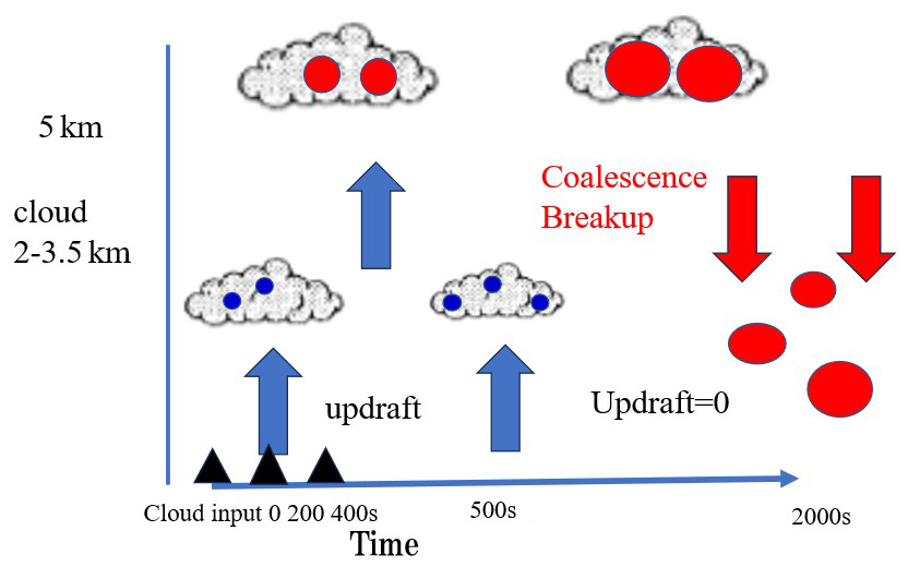
Figure 2 shows a scatter plot of D_m and rain rate calculated for all altitudes, time from 0 to 2000 s and for various initial clouds of D₀ and W₀. Red circles are for W₀=5 m s⁻¹, D₀ of initial cloud as 0.2 mm, black dots are (D₀=0.2 mm) for W₀=10 m s⁻¹. As rainfall rate increases, D_m tends to be constant about 2–2.5 mm for W₀=10 m s⁻¹, which is considered to be an equilibrium state (Ma et al., 2019). Note the equilibrium DSD is independent of the initial characteristics of cloud. The equilibrium state cannot be reached for W₀=5 m s⁻¹. For D_m smaller than the equilibrium size, the envelope of data (D_m) is positively correlated with rainfall rate, whereas negatively correlated for D_m larger than the equilibrium size. This relationship is similar to the relationship between D₀ of rain and rainfall rate for one convective rain measured with the polarimetric radar S-band and a disdrometer (Bringi et al., 2003), which suggests that the Monte Carlo model succeeded in producing similar variations of DSD to the actual rain. Data in the positive correlations, i.e., area of D_m smaller than the equilibrium size may be in developing stage or dissipating stage. Whereas data in the negative correlations, i.e., area of D_m larger than the equilibrium size may indicate few large raindrops in the onset of rain. Large raindrops in upper layer fall rapidly due to sedimentation without suffering breakup.

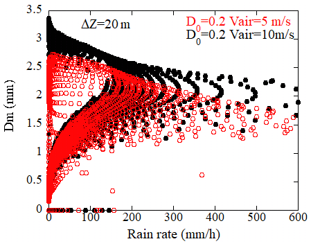
Figure 2 Scatter plot of rain rate and the mass-weighted mean diameter simulated for convective rain. Data for various initial conditions and vertical air motions are plotted.

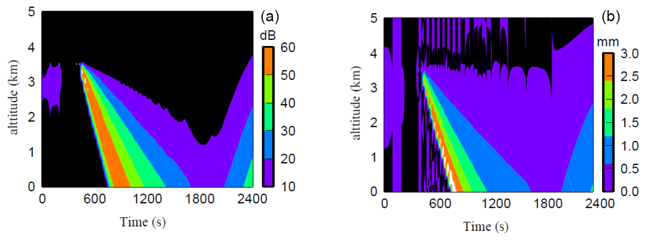
Figure 3 Time-height cross sections of simulated the Rayleigh reflectivity factor Z_e (a) and D_m (b) for convective rain.

Figure 3 shows time-height cross section of Z_e (a) and D_m (b). A precipitation core (here assumed to be an area of Z_e larger than 30 dBZ) descends from 3.5 km to the ground. The peaks of Z_e appear at time of a little later than the time that the core was firstly observed at each altitude. Tendency of D_m is similar to Z_e but the peaks appear at the beginning of core i.e., before Z_e reaches its maximum. This suggests that larger and fewer raindrops descend more rapidly than smaller raindrops without breakup which results in large D_m and small Z_e at the beginning of rain. Similar tendencies have been reported from

the ground-based radar measurements. The time-height cross section of Z_e and the differential reflectivity Z_dr in the precipitation core of convective rain observed by the dual-polarimetric radar shows that the time of the peak of Z_dr appears earlier than the peak of Z_e (Shusse et al., 2015). The differential reflectivity is a measure of the characteristic size of DSD (Bringi et al., 2009), and therefore the tendency is consistent with the present calculations. The simulated results are well representative of the characteristics of the actual rain.

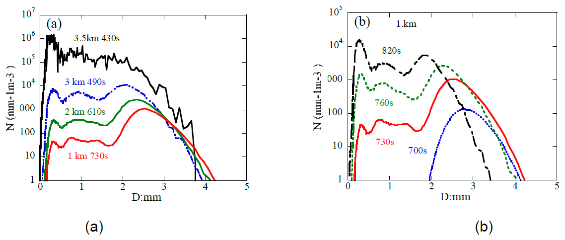
Figure 4 Vertical variation of DSD in the core region (a) and temporal variation of DSD at altitude of 1 km (b).

Figure 4 shows the vertical variation of DSD in the early stage of region (a) shows that higher concentrations of larger raindrops appear in lower altitudes. The temporal variations of DSD at altitude of 1 km (b) shows large drops appear in the early stage of rain and smaller raindrops increase with time at altitude of 1 km.

Figure 5 shows the temporal variations of Z_e, and D_m at an altitude of 0.5 km. This figure clearly shows the difference in the time that the peak of Z_e and D_m appear as shown in Fig. 3. The largest D_m appears at time 720 s whereas the maximum Z_e appears at 810 s. Before 810 s, D_m begins decreasing but Z_e still increases (negative correlation between D_m and Z_e) and after 810 s both D_m and Z_e decrease (positive correlation). Opposite correlations appear between Z_e and D_m. The simulated DSDs show many larger raindrops and few small drops in lower altitudes at the beginning of rain whereas the different shape of DSD appears later. Figure 6a shows the scatter plots of D_m versus Z_e at the time before the core center (time of the maximum Z_e) (red circles), at the core center (black squares) and after the core center (blue triangles) for a vertical velocity of W₀=10 m s⁻¹ and an initial cloud of D₀=0.2 mm. The correlation between Z_e and D_m is positive for D_m<2.5 mm, but negative for D_m>2.5 mm as shown in Fig. 5. At D_m=2.5, values of Z_e converge to high values of about 55 dBZ suggesting the equilibrium state. A similar tendency is obtained in the relationship between Z_e and rainfall rate. For weak updraft of W₀=5 m s⁻¹, no clear positive or negative correlation is obtained. This is due to the insufficient development of raindrops in the upper altitudes.

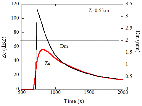
Figure 5 Temporal variations of the Rayleigh reflectivity factor Z_e, and D_m at altitude of 0.5 km.

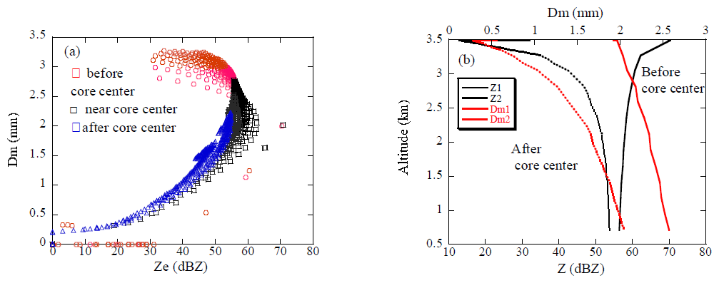
Figure 6 Scatter plots of D_m versus the Rayleigh reflectivity factor Z_e. Data at the core center (black), before (red), and after (blue) the time of core center are plotted (a). Vertical profiles of Z_e and D_m before (Z₁, D_m1) and after (Z₂, D_m2) the time of core center (b).

Figure 6b shows the vertical profiles of Z_e and D_m at time before and after core center. At time before core center, D_m increases toward the ground whereas Z_e tends to decrease indicating large raindrops evolved in upper layer fall due to sedimentation without collision. Decrease tendency in Z_e indicates fewer drop concentration in the lower altitude. Hereafter the raindrop size distribution in this period, referred as “DSDonset”. After the time of core center both D_m and Z_e increase toward the ground due to coalescence and breakup. Since the relationships of D_m−Z_e and Z_e−R change associated with the variations of DSD in life cycle of rain, the relationships can be used to identify the precipitation stage. This is important for accurate rainfall rate estimate, in particular for initiate of rain when estimating rainfall intensity from Z_e. The GPM-core satellite, equipped with dual-frequency radars, measures vertical profiles of Z_e and D_m. As mentioned, vertical variations of D_m are negatively related to Z_e at the beginning of rain in convective rain and D_m is positively correlated to Z_e in mature and dissipating stages. While it is possible to determine the life stage of rain based on the trend of the correlations between Z_e and D_m in altitude, further verification is needed. In addition, realistic temporal and vertical variations of simulated DSD in a convective rain throughout the life cycle are useful to examine a method to estimate D_m from space-borne Doppler radars.

4 A method to estimate D_m from space-borne Doppler radars at Ku-band

The values of D_m are currently derived from the differential frequency ratio (DFR) measured with the Dual-frequency radar onboard the GPM core satellite. In the PMM, a single-frequency Doppler radar operated at Ku-band is currently planned. The EarthCARE satellite also equips a cloud profiling Doppler radar which operates at a single frequency of W-band. For these radars, the characteristic size of raindrops may be expected to estimate from the measured Doppler velocities instead of the DFR technique. The fall velocity of rain drops depends on the size, therefore D_m can be basically derived from the Doppler radars. There are, however, some problems to be solved in the retrieval of D_m. Here, we describe a method to estimate D_m from the space-borne Doppler radars.

The measured mean Doppler velocity (V_p) depends on DSD, the wavelength of radar (λ) and the air motion, and is given by

$$\begin{array}{}\text{(3)}& V_{\mathrm{p}}\left(\mathit{\lambda }\right)={\displaystyle \frac{{\int }_{\mathrm{0}}^{\mathrm{\infty }}{\mathit{\sigma }}_{\mathrm{b}}\left(D\right)N\left(D\right)V_{\mathrm{f}}\left(D\right)\mathrm{d}D}{{\int }_{\mathrm{0}}^{\mathrm{\infty }}{\mathit{\sigma }}_{\mathrm{b}}\left(D\right)N\left(D\right)\mathrm{d}D}}+V_{\mathrm{air}},\end{array}$$

where σ_b is the backscattering cross section, V_f is the fall velocity of raindrops and V_air, is the atmospheric vertical velocity. Given DSD, V_p and D_m correspond one-to-one. In addition, the measured Doppler velocity is affected by the air motion. Thus, in the estimate D_m from V_p, following issues should be considered:

1. The observed Doppler velocity is the sum of the reflectivity-weighted fall velocity of raindrops (V_D) and the atmospheric vertical velocity V_air, it is, therefore necessary to reduce V_air from V_p.

2. Since the measured Doppler velocity is a reflectivity-weighted value, some information on the DSD or assuming DSD are needed.

The effect of (1) is more significant than (2) because the dependence of D_m on V_p is generally larger than the dependence of the DSD. In a convective rain, a strong updraft air motion will be found in the initial stage of rain and downdraft air motion will be found when raindrops are falling. The turbulence also leads to up or down draft. Even small atmospheric velocities (e.g., 0.25 m s⁻¹) can cause large errors in the D_m estimated from V_p in particular for large size of raindrops (Mroz et al., 2020). To reduce the effects of air motion, methods have been developed by using ground-based multi-frequency Doppler radars (Williams et al., 2016; Mroz et al., 2020; Matrosov, 2017). Another approach is to use statistical relationship between the amplitude of Z_e and V_D (e.g., Kollias et al., 2023). A method to estimate V_air from the vertical profiles of Z_e and V_p has been also developed for the EarthCARE (Sato et al., 2009). Statistically, increases in the amplitude of Z_e are associated with V_D, i.e. D_m (e.g., Chen et al., 2022). For stratiform rain or cloud of small variability in the DSD, the effect of (2) may be less significant. However, as mentioned in the previous section, significant variations of the DSD are found in the convective rain, therefore the effect of (2) cannot be ignored.

To address these issues, another approach was applied in the method. Because three parameters of V_air and the DSD (concentration and shape of the DSD) are unknown, another parameter except for Z_e, V_p is needed to estimate D_m. Space-borne radars measure the path-integrated attenuation (PIA) which is the attenuation of radio wave from the surface to the satellite in the presence of precipitation. In the rainfall algorithm of the space-borne radar, the measured PIA is converted to the specific attenuation (k) at each altitude (Meneghini and Nakamura, 1990; Seto et al., 2021) and is used for the attenuation correction. In the method, the specific attenuation is used to specify and reduce V_air and to consider the effects of the DSD. The detailed algorithm will be shown later. Note that the attenuation-corrected reflectivity factors and the specific attenuation are assumed to be given.

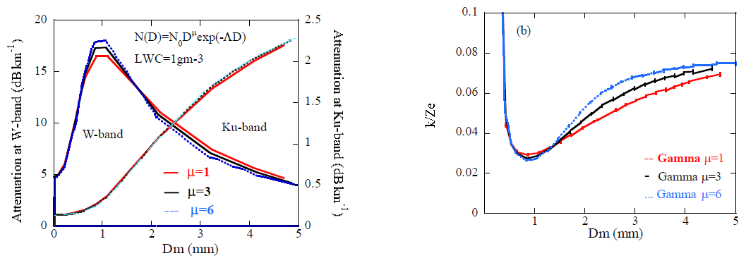
Figure 7 Specific attenuation vs D_m for the DSDs of the Gamma function (a). Various values of the shape parameter μ (1, 3, 6) are plotted for the W and Ku-band. The ratios $k/Z_{\mathrm{e}}$ vs D_m are plotted for various values of μ at the W-band (b).

For the Rayleigh regime, the specific attenuation does not depend on the shape of DSD significantly but is almost determined by the LWC, whereas, k depends on the DSD to some degree as well as LWC for the Mie regime. These features are shown in the relationships between k and D_m (Fig. 7a) for the gamma size distribution of μ=1, 3, and 6 at W and Ku-band, suggesting that k can be used to specify the effects of DSD in the retrieval of D_m from V_p for W-band. For Ku-band, k is not so sensitive to the DSD and is not so effective to identify DSD but is useful to determine the effects of V_air as well as for W-band. Because significant variations of the DSD at large raindrops appear in a real rain, k is useful to identify DSD to some degree even at Ku-band. The values of k are related to Z_e and D_m and can be used to specify the effects of V_air on the retrieval. Figure 7b shows the ratio of k/Z_e which is itself the DSD indicator, and suggests that k is useful to identify the shape (μ) of DSD to some degree except for D_m smaller than 0.5mm.

For the Mie regime, the sensitivity of k to the DSD leads to difficulties in the estimation. The amplitude of k increases monotonically with D_m in the Ku-band, whereas the amplitude of k increases with D_m, reaching a maximum at approximately D_m=1 mm, and then decreases in the W-band. It is, therefore, difficult to determine the exact values of D_m from k. Furthermore, the Ku-band radar on the GPM can measure rain of a high reflectivity as 50 dBZ, whereas signals measured with the W-band attenuates quickly and drops below sensitivity at higher rain rates, so reliable retrievals are not expected above roughly 5–10 mm h⁻¹, not that the instrument is blind to heavier rain. The KuDPR (Ku-band) is a radar to measure precipitation, whereas the CPR operated at W-band is a radar to primarily measure cloud. Considering these differences, the method to estimate D_m at the Ku-band radar will be firstly described. Next, the modified method for W and Ka-band radar s will be presented to examine the potential of the CPR in the measurements of rain. In estimating D_m, attenuation-corrected reflectivity factors are assumed. The validation of the method will be made by using the realistic DSD variation simulated in convective rain as mentioned in the previous section.

4.1 A method for the Ku-band radar

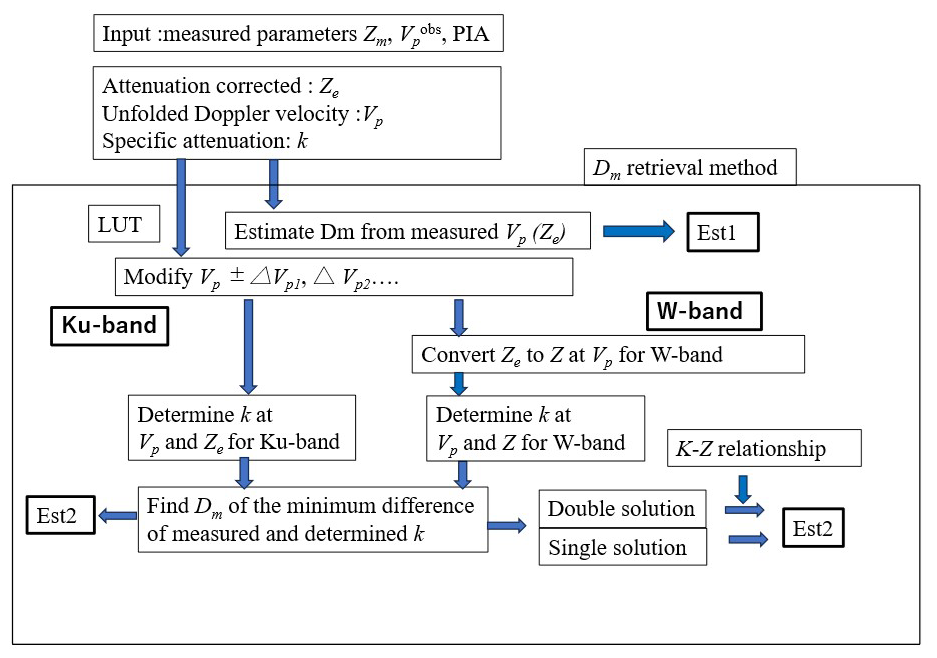
To assess the sensitivity of D_m to the Doppler velocity and k, we performed calculations for various DSDs by Mie theory. Figure 8 shows the representative calculations of the relationships between the measured reflectivity factor (attenuation corrected values Z_e and the Doppler velocity V_D (=V_p in the absence of atmospheric motion) for various values of D_m and k at Ku-band. Data calculated for DSD of the three-parameter Gamma function of μ=3 (Eq. 2) are plotted. The horizontal lines represent Z_e and V_D that result for specified values of k and the vertical lines represent the values for specified values of D_m. The circle symbols shown in the figure represent the simulated values of Z_e and V_p in the convective rain (for LWC <0.1 gm⁻³) as mentioned in the previous section. This figure clearly illustrates a method for the simultaneous determination of D_m and k from the measured values of Z_e and V_p. However, as mentioned earlier, in the presence of air motion, the estimated values of D_m and k will be incorrect. Our object is to estimate D_m, therefore, the value of k obtained from the PIA is used as a parameter to constrain the effects instead of a parameter to be estimated. The values of D_m and V_D can be directly estimated from the measured (attenuation-corrected) Z_e and k, given the DSD. In the actual estimation, first determine D_m and k from the measured Z_e and V_p. In the presence of air motion, incorrect values of D_m and k are obtained. Then, change V_p and determine D_m and k again. Repeat this process until the estimated k matches the observed value and determine the correct value of D_m. Although D_m and V_D can be directly obtained from Z_e and k, given the DSD, this process was applied because the similar process was used for the W-band (4.2), which may be useful for determining whether there is strong air motion.

The Gamma function is often assumed for the DSD in the radar observations and the values of μ=3 is used in the rain-rate estimate algorithm (Seto et al., 2021; Adachi et al., 2015). However, such DSD is not true in a real rain as shown in Fig. 4, In addition, the relationship between D_m and V_p depends on the parameter μ as well (Battaglia et al., 2019). The actual raindrop size distribution is not accurately represented by the gamma function. Accurate estimation results can be expected by selecting a parameter μ in the gamma function whose V_p−D_m relationship is similar to the observed one. In this section, the the look up table (LUT) assuming the values of μ=3 is used to retrieve D_m which is often used in the radar measurements of rain (e.g., Iguchi et al., 2000). The fixed value results in bias errors depending on the DSD in measurements at Ku-band. The LUT with more appropriate μ may be needed which will be discussed in Sect. 4.3. The steps for the retrieval are as follows:

1. Estimate D_m from the measured V_p using the LUT (Fig. 8) (Est1).

2. Estimate k from the measured V_p and the attenuated corrected Z_e using Fig. 8.

3. If estimated k differs from the measured value, estimate D_m and k again by changing V_p as V_p±ΔV_p. The value of ΔV_p was initially set, e.g., to be 0.1 m s⁻¹.

4. Estimate k for various values of ΔV_p and select ΔV_p that gives the minimum difference between estimated k and the measured k.

5. The optimum D_m is determined (Est2).

If the actual DSD is close to the DSD applied in Fig. 8 and in the absence of air motion, selected V_p coincides with V_D, i.e., uncorrected D_m (Est1) coincides with the corrected value (Est2).

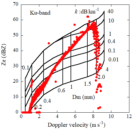
Figure 8 Theoretical relationships between Z_e and the Doppler velocities for various values of D_m and k for the Gamma DSD at the Ku-band. Simulated data in a convective rain are also plotted (red circles).

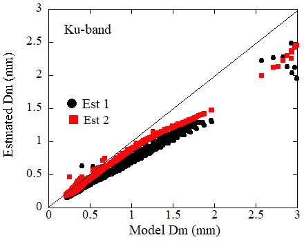
Figure 9 Comparisons of the estimated D_m with the model values at the Ku-band for convective rain (W₀=10 m s⁻¹). Estimated D_m without correction (black circles: $D_{\mathrm{m}}^{\mathrm{Est}\mathrm{1}}$) and with correction (red squares: $D_{\mathrm{m}}^{\mathrm{Est}\mathrm{2}}$) are plotted.

Validation of the retrieval was made using the DSDs at various altitudes and times evolved by the Monte Carlo model. The Doppler velocities, reflectivity factors, specific attenuations and D_ms were calculated from the DSDs and were used for the validation. In Fig. 9, the retrieved D_m values are plotted against calculated (model) values of D_m from the DSDs for W₀=10 m s⁻¹. The vertical velocities of the atmosphere are zero for most data. The black circles represent the uncorrected values of D_m ($D_{\mathrm{m}}^{\mathrm{Est}\mathrm{1}}$), i.e., estimated from the calculated (observed) V_p. The red square symbols represent values of D_m ($D_{\mathrm{m}}^{\mathrm{Ets}\mathrm{2}}$) estimated from Z_e, k and the modified V_p using the LUT. Data of Z_e<50 dBZ are plotted. The uncorrected values $D_{\mathrm{m}}^{\mathrm{Est}\mathrm{1}}$ are underestimated in particular for large values of D_m. Whereas, $D_{\mathrm{m}}^{\mathrm{Ets}\mathrm{2}}$ are closer to the model values. These data are thought to be in still air, so that the reason of the discrepancies is the differences of the measured (simulated) DSD from the DSD applied in the LUT. One of measures to identify DSD is a relationship between the Doppler velocities and D_m which depends on the shape of DSD. Figure 10 shows relationships of V_p and D_m (black square: W₀=3 m s⁻¹, red: 10 m s⁻¹) calculated from the simulated DSDs. The relationships for various Gamma DSDs of μ=1 (blue line), 3 (red) and 12 (green) are also plotted. The simulated values of V_p are smaller than the those of the Gamma DSD. When the relationships of the simulated data of V_p and D_m are fitted by the Gamma function, the fitted values of μ may be larger than 3. For DSD of the Gamma function, V_D tends to increases with decreases in the parameter μ at specified values of D_m for the Rayleigh regime (Williams et al., 2016; Mroz et al., 2020). This indicates that the uncorrected $D_{\mathrm{m}}^{\mathrm{Est}\mathrm{1}}$ will be underestimated if the fitted parameter μ of the DSD in the measurement is larger than that of the LUT and vice-versa. The errors in the corrected values of $D_{\mathrm{m}}^{\mathrm{Ets}\mathrm{2}}$ are significantly reduced but are still underestimated. This is because the correction using the attenuation is not so effective to identify DSD for the Rayleigh scattering as mentioned earlier. Figure 11 is the same as Fig. 9 but for simulated DSD for initial upward air velocity W₀=3 m s⁻¹. In this case, relationship of V_p and D_m is closer to that of the LUT (μ=3) for small values of D_m but larger for D_m>0.5 mm. The corrected values $D_{\mathrm{m}}^{\mathrm{Est}\mathrm{2}}$, are therefore less underestimated and overestimated at D_m=0.5 mm. Errors increase with D_m. Note the points at D_m larger than 2.5 mm in Fig. 9 are for the DSDonset where significant different DSDs appear. Estimated values of D_m from the look-up table of μ_table=1, 3 and 6 are compared (Fig. 12). Symbols of black circles are $D_{\mathrm{m}}^{\mathrm{Est}\mathrm{1}}$, green squares are $D_{\mathrm{m}}^{\mathrm{Est}\mathrm{2}}$ using the LUT of μ_table=1, red circles are estimated from μ_table=3, and blue triangles are estimated from μ_table=6. Corrected values from μ_table=6 are still underestimated but are shown to be improved. The reason of this is that the shapes of the simulated DSDs are similar to the Gamma function of larger values of μ than that of μ_table=3. This figure suggests that selection of appropriate LUT is critical for accurate estimation. This issue will be discussed in Sect. 4.3.

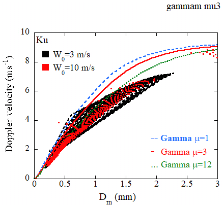
Figure 10 Relationships of D_m and the Doppler velocities of simulated DSDs (black square: W₀=3 m s⁻¹, red: 10 m s⁻¹) and of the Gamma function (blue: μ=1, red: μ=3, green: μ=12).

Figure 11 As in Fig. 9 but for data of W₀=3 m⁻¹.

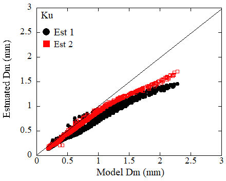
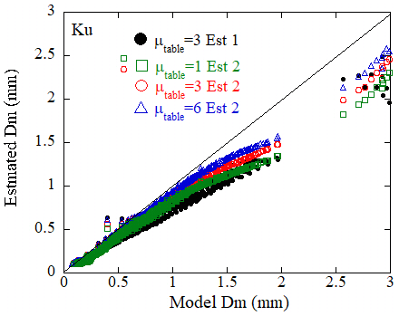
Figure 12 As in Fig. 9 but the retrieved D_m using the look-up table of μ_table=1, 3 and 6 are compared.

4.2 A method for the W-band radar

In the previous section, the method to estimate D_m for the Ku-band Doppler radar was described. The specific attenuation monotonically increases with D_m at this frequency. Whereas, the amplitude of k increases with D_m, reaching maximum at about D_m=1 mm, and then decreases for W-band (Fig. 7). This is because that received signals from the CPR operated at the W-band are almost in the Mie regime while those for Ku-band are almost in the Rayleigh regime. This feature requires the modification of the method for W-band. In this section, we will show the modified algorithm to derive D_m and examine the potential of the method in the measurements of rain with the CPR.

Figure 13 As in Fig. 8 but for W (a) and Ka-band (b).

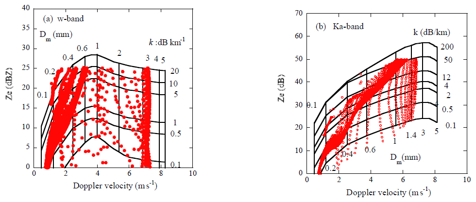
Figure 13 is the same as Fig. 8 but for the W-band (a) and Ka-band (b). The space-borne Ka-band Doppler radar is not currently planned but is added to examine the method for more frequencies. The DSD is assumed to be the gamma function of μ=3 as in Fig. 8. The horizontal lines represent Z_e and V_D that result for specified values of k and the vertical lines represent the values for specified values of D_m. For W-band, the horizontal lines increase with V_p below about 4 m s⁻¹ and then slowly decrease because of the Mie effects. Unfavourable features of Fig. 13a are that two possible solutions can arise for the estimated D_m when determining the optimum value of D_m by varying V_p. Furthermore, the slight change of k with V_p above about 4 m s⁻¹ need considerable high accurate observations of k. Similar features are also shown for Ka-band (b). To avoid such difficulties, the radar reflectivity factor (Z: Z_e for Rayleigh regime) instead of Z_e for W and Ka-band is used. The reflectivity factor Z is determined from the measured Z_e and V_p ±ΔV_p using the LUT. This may lead to additional errors in the estimation. We, however, decided to this method to avoid uncertainties in the use of Z_e mentioned above. For D_m<1 mm, Z_e can be directly used, but Z is used for whole D_m in this study. Generally, Z is linearly related to Z_e for near the Rayleigh regime. For W-band, however, the relationship of Z and Z_e is not simple. The reflectivity factor Z is linearly related to Z_e for Z_e<30 dBZ depending on DSD but is considerably larger than Z_e for larger D_m. This may not be serious because the reflectivity measured with the W-band radar caps around 20–25 dBZ (Z: 20–50 dBZ depending on D_m) as mentioned earlier but is serious for some cases such as DSD of small number concentrations with large rain drops.

To convert the measured reflectivity (attenuated corrected values) to Z, the lookup-tables were prepared for Z, Z_e and V_p for DSD of the gamma function of μ (e.g., 3). The reflectivity factor Z corresponding to the measured Z_e is calculated from the measured Z_e and V_p using the table for various values of D_m. Note that unknown values of D_m are not used for the conversion.

In the presence of strong updraft or downdraft, larger values of ΔV_p is needed to correct the effects of air motion. The values of Z converted from the measured Z_e and V_p ±ΔV_p will also fluctuate significantly. The Z corresponding to the observed Z_e cannot be considered constant and will also vary considerably which sometimes results in multiple solutions. To select the appropriate solution, a k–Z relationship will be used. This issue will be described in Sect. 6 in detail.

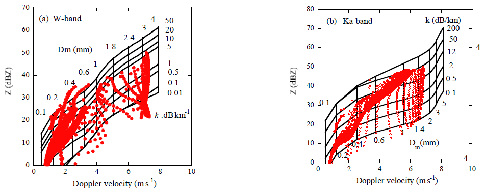
Figure 14 As in Fig. 13 but the Rayleigh scattering equivalent reflectivity factor Z is used instead of Z_e.

Figure 14 is the same as Fig. 13 but for Z. The horizontal lines increase monotonically even for W-band. The circle symbols shown in the figure indicate the simulated values of Z and V_p in the convective rain (for LWC >0.1 gm⁻³). The DSD's that evolved from the weak initial upward velocities as W₀=3 and 5 m s⁻¹ are plotted instead of 10 m s⁻¹ for Ku-band. Smaller reflectivity factor than 25 dBZ which are usually observed with the space-borne W-band radars and 40 dBZ for Ka-band, are shown. From these figures, D_m can be determined from the measured Z_e, k and Z similar to the process for Ku-band. Changing the measured Doppler velocity and find the optimum value of V_p at which the estimated k matches the observed value. Figure 15 shows the flow of the retrieval algorithm.

Figure 15 Retrieval algorithm flow diagram of D_m.

The Ku-band Doppler radar can detect heavy convective rain up to Z_e=40–50 dBZ. Simulated data for the initial updraft velocity of 10 m s⁻¹ are appropriate and were used for the validation. Whereas, retrievals of D_m for W-band radar are limited to light rain of Z_e about 20 dBZ and near top of intense rain layer. Validation was therefore performed using the simulated data of the initial upward velocities of 3 and 5 m s⁻¹for which DSDs of many weak rain events appear. Figure 16a is a similar relationship to Fig. 2 but shows the scatter plots of the measured Doppler velocities (V_p) and the reflectivity factors (Z_m) from the CPR. Most Z_m are less than 20 dBZ even for higher values of V_p. Note that values without attenuation correction and unfolding correction are plotted. Therefore, the Doppler velocities are limited to the Nyquist velocity of 5–6 m s⁻¹. When applying the method to the W-band radar measurements, V_p needs to be unfolded before retrieval of D_m. Figure 16b is the same as Fig. 16a but shows the scatterplots of V_p and Z_e calculated from the simulated DSDs. The data of Z_e less than 25dBZ are plotted. For these weaker W₀, the DSDs similar to the CPR measurements except for higher values of V_p are obtained. These data were used for the validation of the retrieval for W-band in which primarily measures weak rain. Simulated data for W₀=10 m s⁻¹ were also used but were limited number for Z_e<25 dbZ.

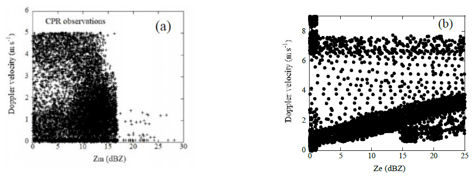
Figure 16 Scatter plot of the Doppler velocities and the reflectivity factor measured with the CPR (a) and simulated (b).

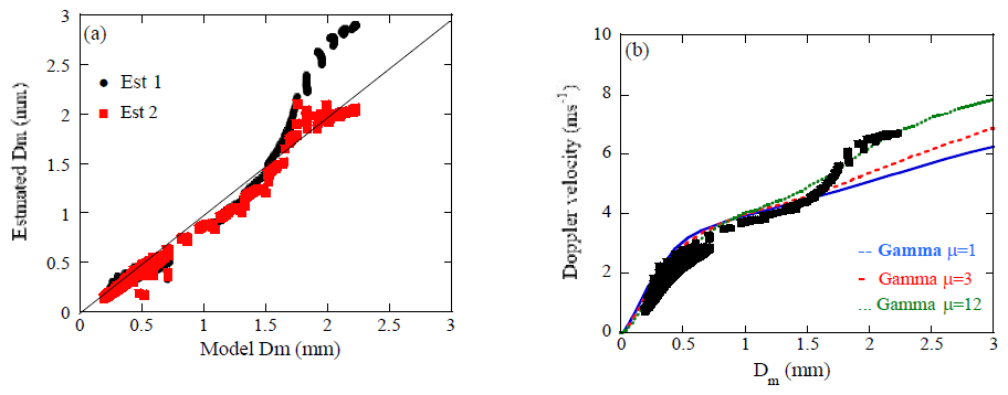
Figure 17 Comparisons of the estimated D_m and the model values at the W-band (a). Estimated D_m without correction (black circles: $D_{\mathrm{m}}^{\mathrm{Est}\mathrm{1}}$) and with correction (red squares: $D_{\mathrm{m}}^{\mathrm{Est}\mathrm{2}}$) are plotted. The Relationships of D_m and the Doppler velocities of the simulated DSDs, and of the Gamma function (μ=1: blue, 3: red, 12: green) are plotted (b).

Figure 17 shows the retrieved and calculated (model) values of D_m for W-band (a). The vertical velocities of the atmosphere are zero for most data. The simulated data with W₀=3 m s⁻¹ are applied. Black circles represent uncorrected values of D_m ($D_{\mathrm{m}}^{\mathrm{Est}\mathrm{1}}$), while red square symbols represent the corrected D_m ($D_{\mathrm{m}}^{\mathrm{Est}\mathrm{2}}$) estimated using the measured values of Z_m, k and V_p. For small values of D_m less than 1.5 mm, both values of $D_{\mathrm{m}}^{\mathrm{Es}\mathrm{1}\mathrm{t}}$ and $D_{\mathrm{m}}^{\mathrm{Est}\mathrm{2}}$ agree well with the model values. However, for large D_m, $D_{\mathrm{m}}^{\mathrm{Est}\mathrm{1}}$ differs significantly from the model D_m. For D_m larger than 1.5 mm, values of $D_{\mathrm{m}}^{\mathrm{Est}\mathrm{1}}$ are overestimated, which is the opposite of the results in Ku-band (Fig. 9). Since these data are considered to be in still air, these discrepancies likely arise from the differences between the measured DSD and the DSD used in the LUT in Figs. 13 and 14. Figure 17b shows the relationships of V_p and D_m obtained from the simulated DSD (black square) which is a measure to identify DSD. The relationships for the Gamma function of μ=1 (blue), 3 (red) and 12 (green) are also plotted. This figure shows that the model values of V_p are significantly larger than the those of the LUT used in the estimation (μ=3) for D_m>1.5 mm, overestimating $D_{\mathrm{m}}^{\mathrm{Est}\mathrm{1}}$ which is opposite to the Rayleigh regime. Despite these deviations, the corrected values of $D_{\mathrm{m}}^{\mathrm{Est}\mathrm{2}}$ significantly reduce errors and agree well with the model values. This is because the method can compensate the effect of DSD on the retrieved D_m to some degree as well as the air motion. The data of large D_m are primarily associated with the DSDonset in which large values of D_m appear in the initial stage of rain and account for less than 5 % of all data.

Figure 18 As in Fig. 17 but for the Ka-band.

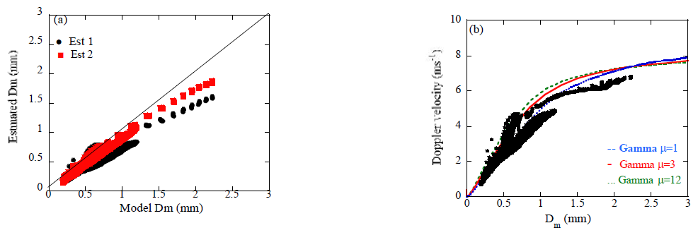
Figure 18 is the same as Fig. 17 but for the Ka-band. Data of W₀=3 m s⁻¹ are plotted. For D_m<1 mm, both estimated values of $D_{\mathrm{m}}^{\mathrm{Est}\mathrm{1}}$ and $D_{\mathrm{m}}^{\mathrm{Est}\mathrm{2}}$ agree well with the model values. However, for D_m>1.5 mm, retrieved $D_{\mathrm{m}}^{\mathrm{Est}\mathrm{1}}$ tends to underestimate which is opposite of the result for W-band but is similar to the result for Ku-band (Fig. 9). In this frequency, the reflectivity both in the Rayleigh regime and the Mie regime coexist depending on the size of raindrops. The errors in the estimated D_m may be small compared with the cases for Ku and W-band. Figure 18b is the same as Fig. 17b but for Ka-band. This figure is similar to the relationship for Ku-band. Smaller values of V_p result in underestimation of $D_{\mathrm{m}}^{\mathrm{Est}\mathrm{1}}$.

4.3 Selection of more appropriate LUT for the Ku-band radar

In the retrieval algorithm, the Mie calculations are performed for the Gamma DSDs of various values of μ to prepare the look-up tables (LUT). In each LUT, values of Z_e, V_p, k, rain rate (R), and $R/Z_{\mathrm{e}}$ for various values of LWC and D_m are stored. Selecting an LUT and estimate D_m. In radar algorithms to estimate rain properties, the Gamma DSD with a value of μ fixed at 3 is often used. This paper also employed such an LUT. This LUT yields generally good estimation results for DSDs of D_m less than 0.5–1.5 mm which are common in many rain events. There are, however, some DSDs of larger D_m than 1.5 mm which result in bias errors in the estimation results. Thus, the accuracy of the retrieved D_m depends on the DSD applied in the LUT. In this section, we will describe a technique to select a more appropriate DSD applied in the LUT to achieve more accurate estimation in the Ku-band radars.

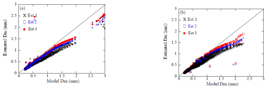
Figure 19 Comparisons of the estimated D_m and model values at the Ku-band for DSDs with W₀=10 m s⁻¹ (a) and W₀=3 m s⁻¹ (b). Estimated D_m without correction (black circles: $D_{\mathrm{m}}^{\mathrm{Ets}\mathrm{1}}$) and with correction (blue squares: $D_{\mathrm{m}}^{\mathrm{Ets}\mathrm{2}}$, red: $D_{\mathrm{m}}^{\mathrm{Ets}\mathrm{3}}$) are plotted.

As shown in Fig. 10, the relationship between V_p and D_m is a measure of DSD and allows estimation of μ close to the actual DSD but cannot be used here. As another measure of DSD, we utilize the dependence of the relationship between Z_e and rain rate on D_m instead. The rain rate will be derived from the measured reflectivity factors and PIA without V_p as in the single frequency algorithm in GPM. In this paper, rain rate was calculated from the simulated DSD. First, estimate $D_{\mathrm{m}}^{\mathrm{Est}\mathrm{1}}$ and $D_{\mathrm{m}}^{\mathrm{Est}\mathrm{2}}$ using the LUT of the initial value of μ (=μ₀). Next, select the ratio of Z_e to rain rate ($Z_{\mathrm{e}}/R$)^LUT for $D_{\mathrm{m}}^{\mathrm{Est}\mathrm{2}}$ from the LUT. The ratio of the measured reflectivity factor and rain rate, ($Z_{\mathrm{e}}/R$)^meas is compared with the ratio ($Z_{\mathrm{e}}/R$)^LUT. If the measured ratio ($Z_{\mathrm{e}}/R$)^meas is larger than the ratio ($Z_{\mathrm{e}}/R$)^LUT of the initial LUT(μ=μ₀), the LUT of larger value of μ (=μ_mod) than μ₀ is selected as a new LUT and vice versa. A new D_m (Est3, $D_{\mathrm{m}}^{\mathrm{Est}\mathrm{3}}$) is re-estimated using the new LUT which is closer to the measured DSD. This process is repeated. Figure 19 shows such estimated $D_{\mathrm{m}}^{\mathrm{Est}\mathrm{3}}$ using a new LUT as well as $D_{\mathrm{m}}^{\mathrm{Est}\mathrm{1}}$ and D^Est2 for DSD of W₀=10 m s⁻¹ (a) and W₀=3 m s⁻¹ (b). The value of μ₀=3, and μ_mod=1, 6 or 9 are used depending on the ratio. Less underestimated $D_{\mathrm{m}}^{\mathrm{Est}\mathrm{3}}$ values appear associated with using more appropriate LUT of larger μ than μ₀. In the estimation, the rain rate calculated from the simulated DSD is applied as mentioned earlier. Note that the rain rate estimate algorithm usually use the measured reflectivity factor and PIA, and is not completely independent of the retrieval algorithm of D_m. The accuracy of this technique depends on the rain rate algorithm and may be needed more validation.

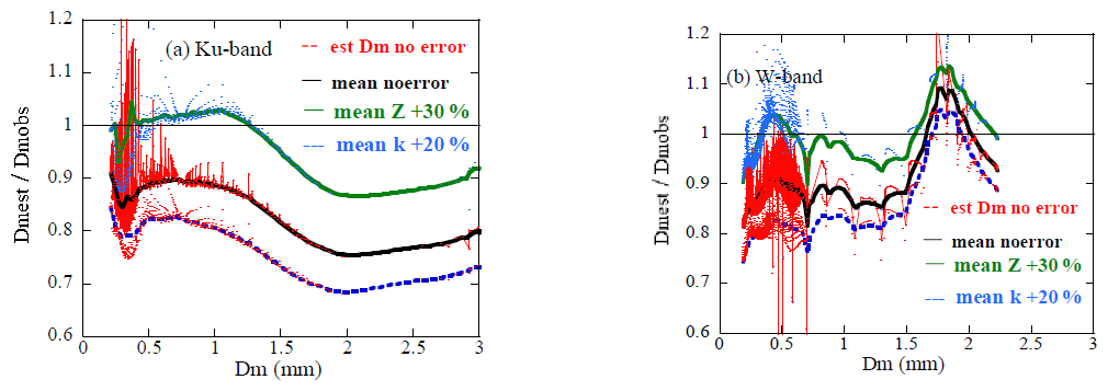
Figure 20 The uncertainties in the estimated $D_{\mathrm{m}}^{\mathrm{Est}\mathrm{2}}$ with and without measurement errors of 30 % in Z_m and 20 % in k at Ku (a) and W-band (b).

5 Error analysis

Having determined D_m, it is important to examine the uncertainties in D_m arising from errors in the measured values and the retrieval process. First, we examine the uncertainties in D_m arising from measurement errors in the reflectivity factors, V_p and k for single solution cases. Even if correct V_p is given, errors in Z_m and/or k result in uncertainties in D_m. Figure 20 shows the uncertainties in the estimated $D_{\mathrm{m}}^{\mathrm{Est}\mathrm{2}}$ with and without measurement errors. The ratios of the estimated D_m to the model values are plotted for Ku (a) and W-band (b). The ratios without measurement errors (black lines) are lower than unity and decrease with D_m for Ku-band. For W-band, the ratios increase sharply at about D_m=1.5 mm. These characteristics are associated with the discrepancies of DSDs in the measurements and LUT in particular for DSDonset. Positive errors in Z_m lead to increases in the ratio and vice-versa for k. The discrepancies between lines with and without measurement errors indicate effects of the measurement errors on the estimation. When there is a 30 % error (linear scale) in Z_m (green line), the ratios increase by 12 % i.e. 12 % errors in the retrieval D_m arising from about 1 dBZ error in Z_m for Ku-band. The effects of the measurement errors of 20 % in k (blue) are smaller as 6 %. For the W-band, there appear smaller effects in particular for larger D_m where larger changes in Z with D_m.

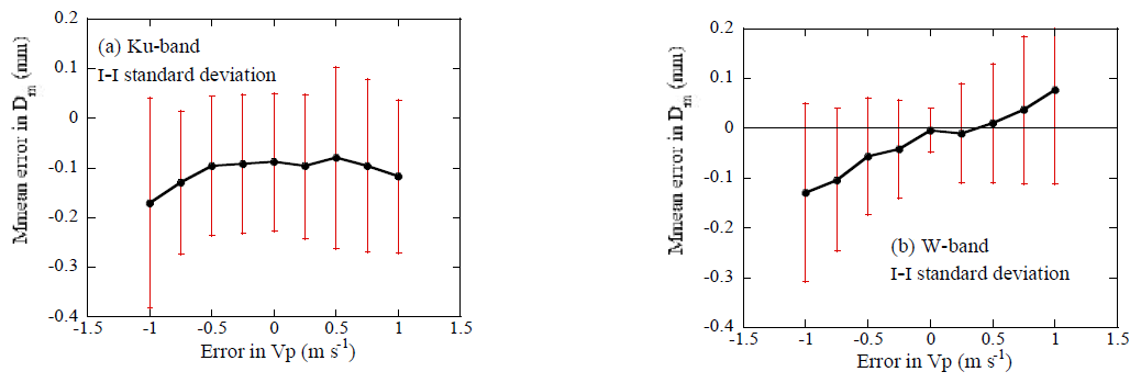
Figure 21 Mean errors in the estimated $D_{\mathrm{m}}^{\mathrm{Est}\mathrm{2}}$ arising from V_p errors for Ku (a) and W-band (b). Uniform random errors in Z_m ranging from −30 % to +30 % and k ranging from −20 % to +20 % are applied.

The errors in V_p are corrected in the retrieval algorithm and do not affect the uncertainties in the retrieved D_m, but may affect the uncertainties when there exist errors in Z_m and k. To assess the uncertainties arising from V_p errors (or air motion), we examined the retrieval errors when uniform random errors in Z_m ranging from −30 % to +30 % and k ranging from −20 % to +20 %. The Conversion of k from PIA may be difficult at W-band. The errors in k depend on range (altitude) and may larger than 20 % in particular at near ground. However, the retrieval of D_m is limited to near top of rain at W-band and therefore less errors are expected. Figure 21 shows the mean errors and standard deviations for various V_p errors. Uncertainties are nearly independent of the V_p errors at the Ku-band (Fig. 21a). At the W-band (Fig. 21b), uncertainties increase with V_p errors due to errors in Z calculating from Z_e. The overall uncertainties are small for V_p errors less than ±0.5 m s⁻¹.

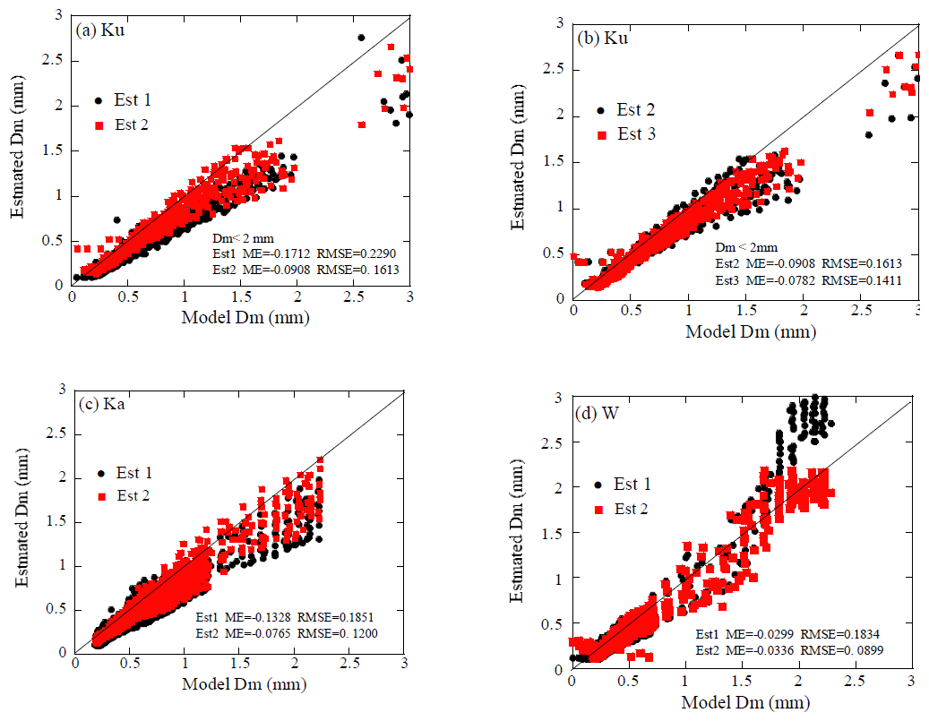
Figure 22 Results of the estimation for random errors in V_p ranging from −0.5 to +0.5 m s⁻¹, Z_e from −30 % to +30 % (about 1 dBZ) and k from −20 % to +20 % uniformly at Ku (a), Ku (b), Ka (c) and W-band (d).

To examine the potential of the method for the practical use, we furthermore estimated D_m when there are random errors in the measured Z_e, k, and V_p. Figure 22 shows comparisons of the estimated and model values of D_m for Ku (a, b), Ka (c) and W-band (d). Results arising from random errors in V_p ranging from −0.5 to +0.5 m s⁻¹, Z_e from −30 % to +30 % (about 1 dBZ) and k from −20 % to +20 % uniformly are plotted. The black circles represent uncorrected values of D_m ($D_{\mathrm{m}}^{\mathrm{Es}\mathrm{1}}$), i.e., estimated from the observed V_p and are not affected the errors in Z_e and k for Ku-band. The red squares represent the corrected $D_{\mathrm{m}}^{\mathrm{Es}\mathrm{2}}$ for panels (a, c, d) and $D_{\mathrm{m}}^{\mathrm{Es}\mathrm{3}}$ for (b). There appears large scatter in the estimated D_m associated with the random errors. Following are the mean error (ME) and the root mean square error (RMSE) of the difference between estimated and model D_ms for Est1, Est2 and Est3.

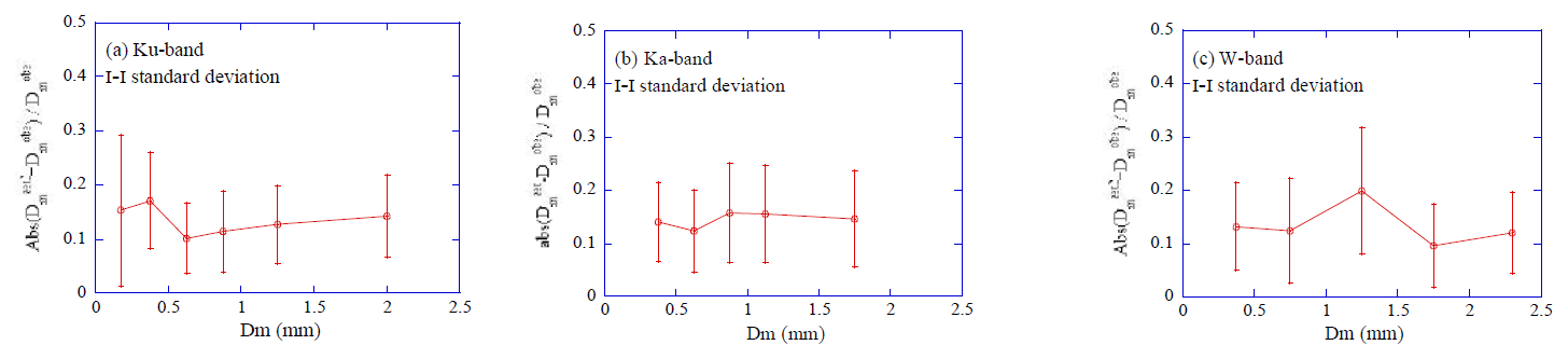
Figure 23 Percentage errors in the retrieved D_m with random errors in Z_e, k, and V_p as in Fig. 22 at Ku (a), Ka (b) and W-band (c). The ratio of the absolute differences between retrieved and model D_m to the model D_m are plotted.

Ku-band:

$$\begin{array}{c}{\displaystyle }{\mathrm{ME}}^{\mathrm{Est}\mathrm{1}}=-\mathrm{0.1712},{\mathrm{ME}}^{\mathrm{Est}\mathrm{2}}=-\mathrm{0.0908},{\mathrm{ME}}^{\mathrm{Est}\mathrm{3}}=-\mathrm{0.0782}\\ {\displaystyle }{\mathrm{RMSE}}^{\mathrm{est}\mathrm{1}}=\mathrm{0.2290},{\mathrm{RMSE}}^{\mathrm{est}\mathrm{2}}=\mathrm{0.1613},{\mathrm{RMS}}^{\mathrm{Eest}\mathrm{3}}=\mathrm{0.1411}\end{array}$$

Ka-band:

$${\displaystyle }\begin{array}{rl}& {\mathrm{ME}}^{\mathrm{Est}\mathrm{1}}=-\mathrm{0.1328},{\mathrm{ME}}^{\mathrm{Est}\mathrm{2}}=-\mathrm{0.0765},{\mathrm{RMSE}}^{\mathrm{est}\mathrm{1}}=\mathrm{0.1851},\\ & {\mathrm{RMSE}}^{\mathrm{est}\mathrm{2}}=\mathrm{0.1200}\end{array}$$

W-band:

$${\displaystyle }\begin{array}{rl}& {\mathrm{ME}}^{\mathrm{Est}\mathrm{1}}=-\mathrm{0.0299},{\mathrm{ME}}^{\mathrm{Est}\mathrm{2}}=-\mathrm{0.0336},{\mathrm{RMSE}}^{\mathrm{est}\mathrm{1}}=\mathrm{0.1834},\\ & {\mathrm{RMSE}}^{\mathrm{est}\mathrm{2}}=\mathrm{0.0897}.\end{array}$$

The mean errors and RMSE in the estimated $D_{\mathrm{m}}^{\mathrm{Est}\mathrm{2}}$ are improved. Uncertainties over the whole range of D_m were relatively small, as shown above. The retrieval errors in D_m, however, vary with D_m because the differences between the measured DSDs and those used in the LUT vary with D_m. Figure 23 shows the percentage errors of the absolute difference between retrieved D_ms and the model values with random errors as in Fig. 22. Mean percentage errors and the standard deviations are plotted for Ku (a), Ka (b) and W-band (c). The mean percentage errors are about 0.15 mm and the standard deviation are less than 0.1 mm. For convective rain, larger vertical velocities often occur than 0.5 m s⁻¹. Effects of such larger air motion on the retrieved D_m will be discussed in next section.

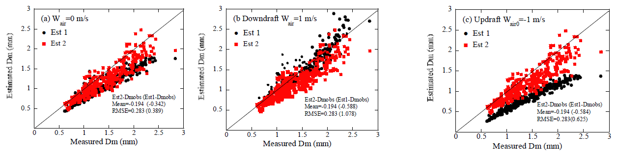
Figure 24 Results of estimating D_m for disdrometer-measured DSDs at the Ku-band with the vertical velocities (W_air) of 0 m s⁻¹ (a), 1 m s⁻¹ (b), and −1 m s⁻¹ (c).

6 Application to disdrometer-measured DSDs

We examined the method for estimating D_m using the DSD evolved from the MonDrop model. Since these DSDs vary significantly both vertically and temporally depending on the stage of precipitation, they are well-suited for validating the method. To estimate D_m, the LUT is prepared in which the DSD is assumed to be a gamma function. The accuracy of the estimated D_m is related to the differences between the observed DSDs and the DSD used in the LUT. Therefore, the validations using actual DSDs allow for more robust assessments of the method's potential and practical use. Here, we examine the retrieval method using disdrometer-measured DSDs at Maebashi, Japan, in July and September 2022. Vertical air motions are added to validate the method. As in Fig. 22, D_ms are estimated by applying random errors that varied uniformly over the ranges of −0.5 to 0.5 m s⁻¹ for V_p, −30 % to 30 % for Z_e, and −20 % to 20 % for k as measurement errors.

Figure 24 shows the results of estimated D_m in the Ku-band with the vertical velocities (W_air) of 0 m s⁻¹ (a), 1 m s⁻¹ (b), and −1 m s⁻¹ (c). Note that negative velocity indicates upward motion. Even in the absence of air motion, the estimated D_ms (Est1) are underestimated, similar to the results shown in Fig. 9. This is likely because the measured DSDs differs from the DSD employed in the LUT. The estimated D_ms (Est2) are closer to the true value. In the case of a downward air motion of 1 m s⁻¹ (b), both Est1 and Est2 are close to the true values due to the effects of the difference between the actual DSD and the DSD_LUT. Conversely, for an upward air velocity of 1 m s⁻¹ (c), the estimated D_ms (Est1) show significantly underestimation due to the reduced values of V_p caused by the updraft air motion, whereas Est2 is not affected by air motion and yields good results.

For the W-band, the measured reflectivity (Z_e) is firstly converted to the Rayleigh reflectivity factor (Z). The Doppler velocities are modified as V_p±ΔV_p so that the calculated specific attenuation using the LUT matches the observed value as mentioned earlier. When the vertical velocities are low (e.g., turbulence), the range over which V_p needs to be varied (ΔV_p) is small, therefore, the fluctuations in Z are small associated with ΔV_p. As shown in Fig. 14, Z increases monotonically with V_p at a specified k, and a single value of D_m can be determined when Z is nearly constant. Since larger values of ΔV_p is needed in the presence of large air motion, the values of Z converted from the measured Z_e and V_p ±ΔV_p will also fluctuate significantly. When the observed V_p differs significantly from the true value (fall velocity of rain drops) due to air motion, the Z corresponding to the observed Z_e cannot be considered constant and will also vary considerably, resulting in complicated variations of k with ΔV_p. The calculated values of k sometimes do not increase/decrease monotonically with ΔV_p and the multiple solution problem arises. There are two or more values of V_ps which give the minimum difference between the calculated k and the observed value.

Figure 25 As in Fig. 24 except for the W-band.

To select the appropriate solution from the multiple solutions as ΔV_p1 and ΔV_p2, the reflectivity factors of Z₁ and Z₂ at ΔV_p1 and ΔV_p2 respectively are used. Generally, Z_e is well collected to k. Similar relationship between Z and k is used to determine Z corresponding to the measured Z_e and k. The appropriate solution is selected from the multiple solutions so that the Zs calculated from the k-Z relationship (Z=ak^b) are closest to the Zs at the multiple solutions. Note that the accurate Z from the k–Z relationship may not be necessary because the reflectivity factors at ΔV_p1 and ΔV_p2 are generally significantly different, given the large difference between ΔV_p1 and ΔV_p2. For the coefficient of the k–Z relationship, the values of a=23.9 and b=0.174 are used for the coefficient of the k-Z relationship which are determined from the empirical formula in the disdrometer data in July. Note that this relationship exhibits larger scatter at smaller Z, so the measured Z is taken to be Z_e for Z less than 20 dBZ.

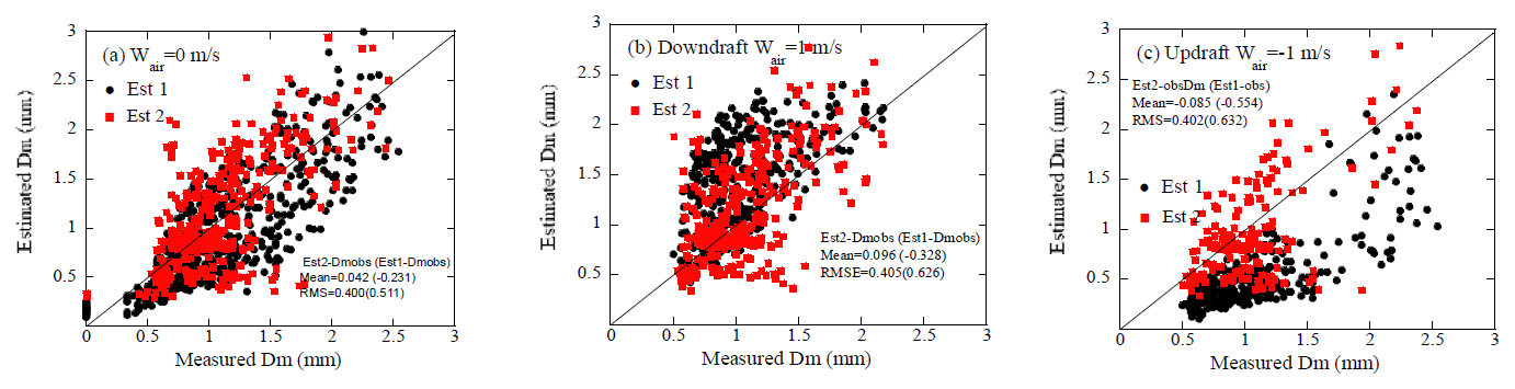
Figure 25 is as in Fig. 24 but for the W-band. For still air (a), the estimated D_ms of Est1 and Est2 seem to be similar results but the mean error is −0.23 for Est1 and −0.042 for Est2. In the presence of downdrafts (b), the estimated D_ms (Est1) overestimate, while they significantly underestimate in the presence of updrafts (c). Conversely, Est2 yields values close to the observed D_m in the both cases. Note Est2 is affected by air motion in this band because Z converted from Z_e is affected by the Doppler velocity.

Figure 26 As in Fig. 24 except for the upward air velocities of 2 and 4 m s⁻¹.

Figure 27 As in Fig. 26 except for the W-band.

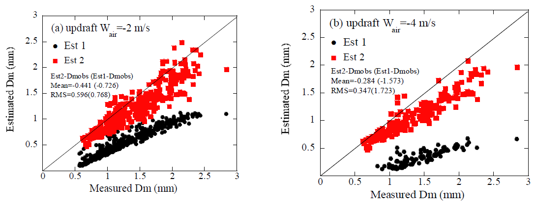
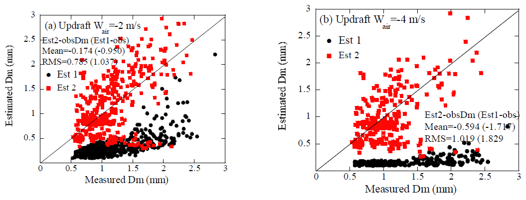
Strong updrafts are often observed in convective rains. We have also estimated D_m for such conditions to examine whether D_m estimations are feasible during convective precipitation with strong updrafts. Figure 26 shows the results for $W_{\mathrm{air}}=-\mathrm{2}$ (a) and −4 m s⁻¹ (b) at the Ku-band. Due to the reduced raindrop fall velocity, D_ms are significantly underestimated for Est1 in particular for $W_{\mathrm{air}}=-\mathrm{4}$ m s⁻¹. Figure 27 is as in Fig. 26 but for the W-band. While the overall tendencies are similar to those of the Ku-band, the estimated D_ms (Est2) exhibit more scatter than that of the Ku-band. This is due to the more complicated retrieval process than that of Ku-band. Mean errors of Est2 are, however, considerably improved. In the presence of large air motion, multiple solutions may arise in the W-band as mentioned earlier. To select the appropriate solution, Z is calculated for each solution using the k–Z relationship. While accurate values of Z from the relationship may not be possible, they may be useful for selecting the appropriate solution. To examine this issue, D_ms were retrieved for DSDs evolved by the MonDrop model using the same k-Z relationship. Figure 28 shows the results of estimating D_m for DSDs (with w₀=3 m s⁻¹) evolved by the MonDrop model in an updraft velocity of −4 m s⁻¹. Some overestimated values of D_m (Est2) appear around D_m=0.6 mm. This is likely because the applied k-Z relationship may not be suitable for certain DSDs generated by the MonDrop model, which exhibit significant variations of DSDs exist. However, the numbers of data with large errors are very limited. Figure 28b shows the frequency histogram of the errors; most data fall within the range of ±0.4 mm, indicating that errors due to the k–Z relationship may be limited.

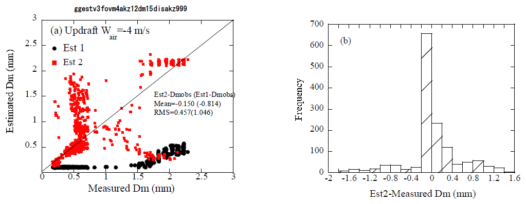
Figure 28 Results of estimated D_m for DSDs evolved by the MonDrop model (W₀=2, 3, 5 m s⁻¹) at the W-band with the vertical velocities of 4 m s⁻¹ (a). Frequency plot of error in Est2 (b).

7 Effects of the variability of DSD

The observed Doppler velocity (V_obs) is the sum of the air velocity (V_air) (Eq. 3) and the velocity (V_D) which is a reflectivity-weighted velocity of raindrop terminal velocity. In estimating D_m, the velocity V_est corresponding to D_m is determined from the LUT (Fig. 8) using measured k and Z_e. Although the difference between V_est and V_obs approximates the vertical air velocity, it is not the exact value because the DSD_LUTusually differs from the actual DSD of raindrops (DSD_obs), resulting in errors in the calculated air velocity and the estimated D_m. The attenuation depends on the shape of DSD but not so significantly. This section discusses whether the measured values of Z_e, k and V_obs, contain the DSD information.

The estimated Doppler velocity of rain fall velocity V_est in estimating D_m, is given as

$$\begin{array}{}\text{(4)}& V_{\mathrm{est}}=V_{\mathrm{D}}+\mathrm{\Delta }{V}_{\mathrm{DSD}}.\end{array}$$

Here, ΔV_DSD represents the error resulting from the difference between the DSD_obs and DSD_LUT. Since k depends on the DSD (Fig. 7), ΔV_DSD is reduced to some extent, but not sufficiently. When the difference between DSD_obs and DSD_LUT is small, the air velocity V_air can be determined by subtracting V_D from V_obs. However, the actual DSD does not usually match the DSD_LUT. Since the exact shape of DSD_obs is unknown, it is difficult to determine the exact ΔV_DSD. Nevertheless, if the parameter (f) characterizing the DSD (such as μ in a Gamma distribution) is known, it is possible to estimate ΔV_DSD to some degree. Using the parameter f, ΔV_DSD can be expressed as:

$$\begin{array}{}\text{(5)}& \mathrm{\Delta }{V}_{\mathrm{DSD}}={\displaystyle \frac{\mathrm{d}V\left(f\right)}{\mathrm{d}f}}\mathrm{\Delta }f,\end{array}$$

where Δf represents the difference between the parameter f_obs and f_LUT which characterize DSD_obs and the DSD_LUT respectively.

Figure 29 shows the relationship between $k/Z_{\mathrm{e}}$ and the Doppler velocity for the gamma functions with various values of μ for W-band. This figure demonstrates that this ratio $k/Z_{\mathrm{e}}$ varies with μ, suggesting that $k/Z_{\mathrm{e}}$ can be used as an indicator of the shape of DSD. When δ($k/Z_{\mathrm{e}}$) is used as the parameter f, Eq. (5) is expressed as:

$$\begin{array}{}\text{(6)}& \mathrm{\Delta }{V}_{\mathrm{DSD}}={\displaystyle \frac{\mathrm{d}V}{\mathrm{d}\mathit{\delta }(k/Z_{\mathrm{e}})}}\left\{{\left({\displaystyle \frac{k}{Z_{\mathrm{e}}}}\right)}_{\mathrm{LUT}}^{V_{\mathrm{est}}}-{\left({\displaystyle \frac{k}{Z_{\mathrm{e}}}}\right)}_{\mathrm{Obs}}\right\}.\end{array}$$

where ($k/Z_{\mathrm{e}}$)${}_{\mathrm{LUT}}^{V_{\mathrm{est}}}$ represents the value of ($k/Z_{\mathrm{e}}$) at V_est for DSD_LUT and ($k/Z_{\mathrm{e}}$)_obs is the measured ($k/Z_{\mathrm{e}}$). Here, δ($k/Z_{\mathrm{e}}$) (where Z_e is a linear scale), which defined as the difference in $k/Z_{\mathrm{e}}$ between different DSDs, is used as the parameter f. As shown in Fig. 7b, $k/Z_{\mathrm{e}}$ depends on DSD, specifically on the μ of the gamma function. The DSD information provided by $k/Z_{\mathrm{e}}$ is limited but was selected because this parameter can be obtained directly from the Doppler radar measurements. To calculate ($k/Z_{\mathrm{e}}$) for various values of V, ($k/Z_{\mathrm{e}}$) of each DSD was approximated using a fourth-order polynomial in V. The values of V_D were determined by iteratively varying the V_D value to satisfy Eq. (4), instead of directly solving the fourth-order equation. The Doppler velocity V_D is derived from ΔV_DSD and V_est.

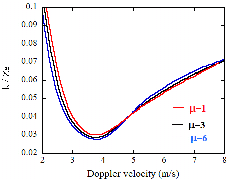
Figure 29 The relationship between $k/Z_{\mathrm{e}}$ and the Doppler velocity for the gamma functions with various values of μ for the W-band.

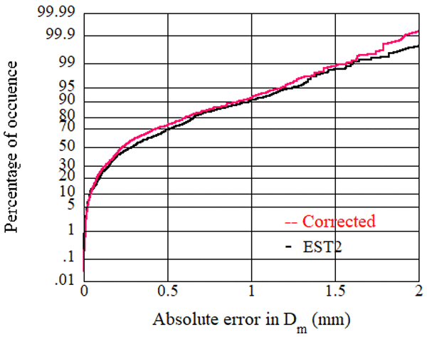
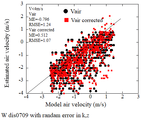
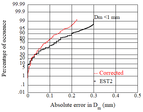
Here, we examine the technique using disdrometer-measured DSDs as shown in the previous section. Vertical air motions are added to validate the method except for the Ku-band. As in Fig. 22, the effects of DSD are evaluated by applying random errors that varied uniformly over the ranges of −0.5 to 0.5 m s⁻¹ for V_p, −30 % to 30 % for Z_e, and −20 % to 20 % for k as measurement errors. Figure 30 shows the estimated vertical air velocities plotted against the true (model) V_air. Black circles are V_air derived from V_est and red squares are V_air derived from V_D, that is corrected the effects of DSD. Although there is significant scatter, both results show good correlation with the model values. The corrected values are slightly improved in the mean error (ME) and the root mean square error (RMSE) but not significantly because ($k/Z_{\mathrm{e}}$) contains limited information of DSD in particular for the Doppler velocity around 5 m s⁻¹. Note that whether the term $(k/Z_{\mathrm{e}}{)}_{\mathrm{LUT}}-(k/Z_{\mathrm{e}}{)}_{\mathrm{obs}}$ or vice-versa in Eq. (6) depends on whether the observed V_obs is larger or less than the value in LUT (Fig. 30). The derived V_Ds were also used to estimate D_m. Figure 31 shows cumulative percentage of the estimated errors of Est2 and D_m from V_D, showing improvement. The cumulative percentage of occurrence of the absolute error less than 0.5 mm is improved by 5 %.

Figure 30 Errors in the estimated and corrected V_air vs the model values.

For Ku-band, k is primarily determined by the LWC of rain rather than the shape of DSD. Consequently, it is difficult to assess the DSD effects by using $k/Z_{\mathrm{e}}$. Here, we examine whether the DSD information provided by the measured values of Z_e. k and V_obs in the Ku-band. In doing so, the parameter ($k{V}_{\mathrm{est}}/Z_{\mathrm{e}}$) is used for f instead of ($k/Z_{\mathrm{e}}$). This may be strange but may be possible because f is a parameter to define the effects of the difference of DSD on V. Figure 32 shows the relationship between $k{V}_{\mathrm{D}}/Z_{\mathrm{e}}$ and the Doppler velocity for DSD of the gamma functions with μ=1 and 3 for Ku-band. This figure suggests that this ratio $k{V}_{\mathrm{D}}/Z_{\mathrm{e}}$ varies with μ for V_D less than 4 m s⁻¹ and can be used as an indicator of the shape of DSD for such range. Figure 33 is the same as Fig. 31 but for Ku-band. The value of V_D less than 4 m s⁻¹ are plotted, showing slight improvement.

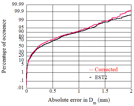
Figure 31 Cumulative percentage of the occurrence of the errors in the estimated D_m (Est2) and the corrected values.

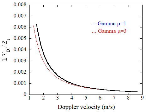
Figure 32 The relationship between $k{V}_{\mathrm{D}}/Z_{\mathrm{e}}$ and the Doppler velocity for DSD of the gamma functions with μ=1 and 3 for the Ku-band.

Figure 33 Same as in Fig. 31 but for the Ku-band.

8 Summary

A physically-based algorithm for estimating mass-weighted raindrop diameter (D_m) from radar reflectivity and specific attenuation is presented. In the absence of the vertical air motion, D_m can be estimated from the Doppler velocity observed by a space-borne Doppler radar, assuming a specific DSD. The estimated D_ms are not correct in the presence of the air motion. A detailed error analysis is presented in estimating D_m ($D_{\mathrm{m}}^{\mathrm{Est}\mathrm{1}}$, $D_{\mathrm{m}}^{\mathrm{Est}\mathrm{2}}$) using simulated rain drop size distributions and disdrometer-measured DSDs. A Monte Carlo model was employed to evolve the DSD through coalescence and breakup in a convective rain.

At the Ku-band, values of D_m were estimated from the attenuation-corrected Z_e and the specific attenuation k, assuming DSD ($D_{\mathrm{m}}^{\mathrm{Est}\mathrm{2}}$). Although errors arising from the discrepancy between the assumed and actual DSDs occur, their magnitude is smaller than $D_{\mathrm{m}}^{\mathrm{Est}\mathrm{1}}$. The effects related to the variability of DSD were difficult to correct due to the Rayleigh scattering regime. Accurate estimation requires appropriate LUTs with the DSD similar to the measured one. A technique to determine more appropriate LUTs was presented by exploiting the dependence of the Z-R relationship on D_m for the Ku-band. The retrieved D_ms were improved using this technique. Additionally, using $k{V}_{\mathrm{est}}/Z_{\mathrm{e}}$ as a measure, that is, a parameter representing the DSD shape may offers a potential way to reduce the DSD effects. At the W-band, D_ms were also estimated. In the estimation, the Rayleigh reflectivity, converted from the measured Z_e using the Doppler velocities was used. Since k depends on the shape of DSD, the DSD-related effects are reduced but are limited. The effects are relatively smaller for small D_m but are larger for larger D_m. The DSD-related effects may be reduced by using $k/Z_{\mathrm{e}}$ as a measure of the DSD shape.

The values of Z_e and k both depend on the same attenuation retrieval, so their errors are correlated. Further efforts are required to measure these values accurately in particular for the W-band. Although the estimation is limited for weak rain or near top of rain layer at the W-band due to significant attenuation and the Mie scattering regime, the presented method possibly improves our understanding of the rain system with space-borne doppler radar.

Appendix A: Method by Gillespie (1975) and Seeßelberg et al. (1996)

Gillespie (1975) defined and calculated a probability function P(τ, i,j) called the coalescence probability density function, and proposed a method that does not ignore the correlation, instead of calculating number of particles directly. Consider the case where there are well-mixed N droplets at time t. The function P(τ, i, j) dτ(i<j) is the probability that droplets i and j will collide in the time interval t+τ and $t+\mathit{\tau }+\mathrm{d}\mathit{\tau }$, dτ is the infinitesimal time. This probability is the product of the probability that no collision occurs in the time interval t, t+τ, the probability that a collision occurs between t+τ and $t+\mathit{\tau }+\mathrm{d}\mathit{\tau }$ and the probability that no collision of the other particle occurs between t+τ and $t+\mathit{\tau }+\mathrm{d}\mathit{\tau }$ and is expressed as follows.

$$\begin{array}{}\text{(A1)}& P\left(\mathit{\tau },i,j\right)=C_{ij}\exp \left[-\sum _{k=\mathrm{1}}^{N-\mathrm{1}}\sum _{l=k+\mathrm{1}}^N{C}_{kl}\mathit{\tau }\right],\end{array}$$

where C_ij dτ the probability that droplets i, j will collide in the next infinitesimal time dτ which is related to the collection kernel as K (m_i, m_j) per the volume of well-mixed cloud or rain. Given C_ij, the probability can be obtained without approximation. The collision process is numerically calculated for an arbitrary kernel. Equation (A1) is given as

$$\begin{array}{}\text{(A2)}& P\left(\mathit{\tau },i,j\right)=C_{ij}\exp \left(-C_{\mathrm{0}}\mathit{\tau }\right),\end{array}$$

where C₀ is the total rate for any collision events in the volume V. In the model by Seeßelberg et al. (1996) in which drop classes are introduced to specify DSD, and C₀ is given as

$$\begin{array}{}\text{(A3)}& C_{\mathrm{0}}\equiv V^{-\mathrm{1}}\sum _{i=\mathrm{1}}^N\sum _{j=i+\mathrm{1}}^N{K}_{ij}{N}_i{N}_j+V^{-\mathrm{1}}\sum _{i=\mathrm{1}}^N{K}_{ii}{\displaystyle \frac{N_i\left(N_i-\mathrm{1}\right)}{\mathrm{2}}},\end{array}$$

where K_ij is the collision kernel, the probability that particles i and j in the volume V collide. The first term on the right-hand side represents the probability that particles i≠j and the second term represents the probability that drops of i=j collide. The time interval τ is determined from Eq. (A2) using uniformly distributed random number (η) from 0 to 1 as:

$$\begin{array}{}\text{(A4)}& \mathit{\tau }=-C_{\mathrm{0}}^{-\mathrm{1}}\ln \mathit{\eta }.\end{array}$$

The next step is to select colliding droplets (i,j). The probability of collision of droplet i and j, (D_ij) is expressed as

$$\begin{array}{}\text{(A5a)}& D_{i,i}\equiv V^{-\mathrm{1}}{K}_{i,i}{\displaystyle \frac{N_i\left(N_i-\mathrm{1}\right)}{\mathrm{2}{C}_{\mathrm{0}}}},i=j\end{array}$$

$$\begin{array}{}\text{(A5b)}& D_{i,j}\equiv V^{-\mathrm{1}}{K}_{ij}{N}_i{N}_j/C_{\mathrm{0}}.i\ne j\end{array}$$

The probability of collision of particle i with any other droplets, D_i is as follows.

$$\begin{array}{}\text{(A6)}& D_i=\sum _{j=i+\mathrm{1}}^N\left[D_{ij,}+D_{ii}\right].\end{array}$$

The colliding particle i is determined from the cumulative distribution of $D_i/C_{\mathrm{0}}$ with respect to droplet i and a random number. The colliding droplet j with drop i is determined from the cumulative distribution of $D_{ij}/D_i$ and a random number. Create a cumulative distribution for the mass (bin number) i of $\sum D_i/C_{\mathrm{0}}$ and determine the mass i by a random number. In this algorithm, the so-called well-known problem (Bott, 1998) arises: the bin of a newly generated particle by coalescence or breakup is determined but is not known the exact size in the bin. We apply the method by Seeßelberg et al. (1996).

The collection kernel is written as follows:

$$\begin{array}{}\text{(A7)}& K\left(r,r^{\prime }\right)=\mathit{\pi }{\left(r{}^{\prime }+r\right)}^{\mathrm{2}}{E}_{\mathrm{col}}{E}_{\mathrm{coal}}\left|V_{\mathrm{\infty }}\left(r\right)-V_{\mathrm{\infty }}\left(r^{\prime }\right)\right|,\end{array}$$

where E_col is the collision efficiency, which is the ratio of collision cross section to the geometric cross section, and E_coal is the coalescence efficiency, which indicates the probability of coalescence of collision particles. In this paper, the collision efficiency is set to be unity considering the fact that the raindrop size is larger than 0.1 mm. The coalescence efficiency was calculated by Low and List (1982a).

$$\begin{array}{}\text{(A8)}& E_{\mathrm{coal}}=a{\left(\mathrm{1}+{\displaystyle \frac{D_{\mathrm{s}}}{D_{\mathrm{L}}}}\right)}^{-\mathrm{2}}\exp \left(-{\displaystyle \frac{b\mathit{\sigma }{E_r}^{\mathrm{2}}}{S_c}}\right).\end{array}$$

Here, D_L and D_s are the diameters of larger and smaller drops, and S_c is the surface energy of the spherical equivalent of the united drop mass. E_r is the sum of the collision kinetic energy and the particle surface energy loss due to coalescence. σ is the surface tension of water. Parameter a and b are constant values. The effect of turbulence is not considered. The coalescence efficiency by Low and List (1982a) may underestimate the coalescence and result in higher slope in the equilibrium raindrop size distribution (Barthes and Mallet, 2013; Hu and Srivastava, 1995). The shape of DSD significantly varies in vertical as well as in the life stage of rain. The object of the simulation is to create a database of such variations of DSD to examine the method for estimating D_m from space-borne Doppler radar observations, therefore the coalescence efficiency of Eq. (A8) which has been usually used, was applied. For breakup, the probabilities of the occurrence of the filament, sheet, and disk types were considered. The DSD of each type of breakup was determined by Low and List (1982b). Note, the rate of breakup was assumed to be (1−E_coal) and for D_L<0.2 mm, E_coal=1.

Finally, we will mention statistical fluctuations of the results of the MonDrop. Statistically accurate results may be obtained from several runs between three to 10 (Gillespie, 1975). To determine statistically meaningful results with K runs, following values are used.

$$\begin{array}{}\text{(A9)}& \mathrm{\Delta }D={\left\{{\displaystyle \frac{\mathrm{1}}{K}}\sum _{i=\mathrm{1}}^K{\left[N_i\left(x\right)\right]}^{\mathrm{2}}-{\left[{\displaystyle \frac{\mathrm{1}}{K}}\sum _{i=\mathrm{1}}^K\left[N_i\left(x\right)\right]\right]}^{\mathrm{2}}\right\}}^{\frac{\mathrm{1}}{\mathrm{2}}},\end{array}$$

where N_i is the Monte Carlo results, such as DSD, LWC, etc. at i run. If $\mathrm{\Delta }D/N_i\ll \mathrm{1}$, the result can be considered reliable.