Algorithms to retrieve aerosol optical properties using lidar measurements on board the EarthCARE satellite

The Earth Cloud Aerosol and Radiation Explorer (EarthCARE) is a joint Japanese-European satellite observation mission for understanding the interaction between cloud, aerosol, and radiation processes and improving the accuracy of climate change predictions. The EarthCARE satellite was equipped with four sensors, a 355 nm high-spectral-resolution lidar with depolarization measurement capability (ATLID) as well as a cloud profiling radar, a multi-spectral imager, and a broadband radiometer, to observe the global distribution of clouds, aerosols, and radiation. In this study, we have developed algorithms to produce ATLID Level 2 aerosol products using ATLID Level 1 data. The algorithms estimated the following four products: (1) Layer identifiers such as aerosols, clouds, clear-skies, or surfaces were estimated by the combined use of vertically variable criteria and spatial continuity methods developed for the CALIOP (Cloud-Aerosol Lidar and Infrared Pathfinder Satellite Observation) analysis. (2) Aerosol optical properties such as extinction coefficient, backscatter coefficient, depolarization ratio, and lidar ratio at 355 nm were optimized to ATLID L1 data by the method of maximum likelihood. (3) Six aerosol types, namely smoke, pollution, marine, pristine, dusty-mixture, and dust were identified based on a two-dimensional diagram of the lidar ratio and depolarization ratio at 355 nm developed by cluster-analysis using the AERONET (AErosol RObotic NETwork) dataset with ground-based lidar data. (4) The planetary boundary layer height was determined using the improved wavelet covariance transform method for the ATLID analysis. The performance of various algorithms was evaluated using pseudo ATLID Level 1 data generated by Joint-Simulator (Joint Simulator for Satellite Sensors), which incorporates aerosol and cloud distributions simulated by numerical models. Results from applying the algorithms to the pseudo ATLID Level 1 data with realistic signal noise added for aerosol or cloud predominant cases revealed: (1) misidentification of aerosol and cloud layers was relatively low, approximately 10 %; (2) the retrieval errors of aerosol optical properties were $\mathrm{0.08}\times {\mathrm{10}}^{-\mathrm{7}}\pm \mathrm{1.12}\times {\mathrm{10}}^{-\mathrm{7}}{\mathrm{m}}^{-\mathrm{1}}{\mathrm{sr}}^{-\mathrm{1}}$ (2±34 % in relative error) for backscatter coefficient and 0.01±0.07 (4±27 % in relative error) for depolarization ratio; (3) aerosol type classification was generally performed well. These results indicate that the algorithm's capability to provide valuable insights into the global distribution of aerosols and clouds, facilitating assessments of their climate impact through atmospheric radiation processes.

1 Introduction

Global measurements of the optical properties of atmospheric particles, encompassing aerosols and clouds, play a pivotal role in evaluating their climatic effects through atmospheric radiation processes. Zhang et al. (2022) analyzed the simulation results of the Coupled Model Intercomparison Project Phase 6 (CMIP6) global models and indicated that 20 % of radiative effect uncertainty for anthropogenic aerosols was associated with aerosol vertical distribution under clear-sky condition. In addition, the presence of highly light-absorbing aerosols such as black carbon above or below the cloud layer can prodoundly the radiative transfer process of the upper atmosphere (Takemura et al., 2002; Oikawa et al., 2013, 2018). The Cloud-Aerosol Lidar and Infrared Pathfinder Satellite Observation (CALIPSO) satellite, equipped with the two-wavelength (1064, 532 nm) polarization Mie-scattering lidar CALIOP (Cloud-Aerosol LIdar with Orthogonal Polarization), has globally measured aerosols and cloud vertical distributions over the long term from 2006–2023 (Winker et al., 2010). This role will transition to ATLID (Atmospheric Lidar) (Heìliere et al., 2017; do Carmo et al., 2021), the 355 nm high-spectral resolution lidar (HSRL) with polarization measurement function onboard the EarthCARE satellite (Earth Cloud Aerosol and Radiation Explorer). EarthCARE is a joint Japan-Europe satellite observation mission by JAXA (Japan Aerospace Exploration Agency), NICT (National Institute of Information and Communications Technology), and ESA (European Space Agency), which aims to conduct comprehensive global observations of clouds, aerosols, and atmospheric radiation (Wehr et al., 2023). The EarthCARE satellite features a 94 GHz cloud radar (CPR) with doppler measurement capability (Nakatsuka et al., 2023), a multiwavelength imager (MSI), comprising seven channels in the visible to infrared wavelength range (Wallace et al., 2016), and a broadband radiometer (BBR) designed for measuring shortwave and longwave radiation (Wallace et al., 2016). The scientific objectives emcompass (1) observing the global vertical distributions of natural and anthropogenic aerosols and their interaction with clouds; (2) observing global cloud distributions, cloud-precipitation interactions, and vertical motion characteristics within clouds; (3) evaluating the vertical profiles of radiative heating and cooling of the atmosphere (Illingworth et al., 2015; Okamoto et al., 2024a).

ATLID, a HSRL, can independently measure backscattered light from atmospheric particles (Mie signal) and backscattered light from atmospheric molecules (Rayleigh signal) separately, distinguishing it from CALIOP, a Mie-scattering lidar. This unique feature allows for the independent extraction of the vertical distributions of the extinction coefficient and backscattering coefficients of atmospheric particles by analyzing these two signals. Moreover, ATLID conducts polarization measurements, enabling the extraction of the co-polar component, parallel to the laser polarization (co-polar component), the cross-polar component (perpendicular to the laser polarization) of the Mie signal at a wavelength of 355 nm, and the Rayleigh signal. Signal calibrations are performed on these measured signals, resulting in calibrated attenuated backscatter coefficients.

Multichannel lidar observations using a combination of polarization measurements, Rayleigh/Mie separation measurements, and/or various wavelength measurements, including those of ATLID, CALIOP, and ground-based lidar measurements, facilitate simultaneous understanding of various optical and microphysical properties of atmospheric particles. This includes the identification of major atmospheric layers such as aerosol or cloud layers (Okamoto et al., 2008; Vaughan et al., 2009; Liu et al., 2009; Hagihara et al., 2010) and the identification of aerosol and cloud types such as marine, dust, warm water, or 2-D ice (Omar et al., 2009; Yoshida et al., 2010; Illingworth et al., 2015; Okamoto et al., 2019). The size distribution and refractive index of total aerosols can be estimated using extinction coefficients and backscatter coefficients at two wavelengths (355 and 532 nm) observed by the Raman lidar and HSRL (e.g., Müller et al., 2014). The extinction coefficients of some major aerosol components (such as mineral dust and black carbon) have been estimated (Nishizawa et al., 2017; Kudo et al., 2023). Understanding of the climate impact of aerosols, necessitates not only comprehending the optical and microphysical properties of total aerosols but also those of individual aerosol components. For example, aerosols with strong light absorption properties (e.g., black carbon) have been reported to influence cloud formation and global atmospheric and water circulations in large fields (Menon et al., 2002; Koren et al., 2004). In addition, the top height of the planetary boundary layer (PBL) has been detected by various methods such as the gradient method (Lammert and Bösenberg, 2006), the wavelet covariance transform (WCT) method (Brooks, 2003), or other methods (e.g., the standard deviation method by Menut et al., 1999). Since aerosols emitted from the surface are trapped within the PBL because of the temperature inversion between the PBL and free troposphere, its top height, by which the transition point of the aerosol concentration gap is characterized, is an important parameter for understanding climate and air quality.

The EarthCARE mission generates Level 1 (L1) products, which are physical quantities derived after calibrating the measurements of each instrument, and Level 2 (L2) products, consisting of geophysical variables related to clouds, aerosols, etc, utilising L1 data either independenally or in combination (Eisinger et al., 2024). Each sensor development organization (JAXA and NICT for CPR, and ESA for others) generates the L1 product, and the L2 product is generated by individual agencies. For example, L2 products using ATLID, such as layer identifiers, particle (aerosol, cloud) type identifiers, and optical properties, such as extinction coefficient, backscatter coefficient, and depolarization ratio, and cloud top height, are estimated by ESA (Irbah et al., 2023; Donovan et al., 2023, 2024; Zadelhoff et al., 2023; Wandinger et al., 2023). Synergy products are also generated by combining L1 data from the other instruments. JAXA also provides various ATLID standalone and synergistic products, while similar to ESA products, are produced using different independent retrieval methods developed independently.

To determine the globally vertical distribution of optical properties of aerosols and clouds needed to assess their climatic effects, we have developed atmospheric particle retrieval algorithms to generate JAXA L2 products using ATLID L1 data. In this study, we focus on the retrieval algorithms and products related to aerosols, whereas the description of cloud property estimation is planned for separate papers. Section 2 describes the products retrieved using the algorithms and their flows. Section 3 describes the algorithms developed to retrieve the individual products. Section 4 presents the products estimated using the simulated input data (ATLID L1 data) and the performance of the various algorithms. In Sect. 5, we summarize and discuss the prospects.

2 Algorithm flow and products

Figure 1 illustrates the products and flow of the algorithms. First, to improve signal quality, the algorithm reduces the signal noise using a discrete wavelet transform (DWT) (Fang and Huang, 2004). In this study, two types of Daubechies wavelets (support numbers 2 (D2) and 4 (D4)) are employed. Noise reduction is performed iteratively with D2, followed by D4, and then the noise reduction using D2 is applied again, followed by D4 and so on ($\text{D2}=>\text{D4}=>\text{D2}=>\text{D4}=>\text{D2}\mathrm{\dots }$). A simulation analysis with added random noise indicated that the applying the DWT method could improve the signal-to-noise ratio (SNR) by a factor of two or more. Therefore, this method was adopted in the present study.

Figure 1 ATLID L2 products and the flow of algorithms.

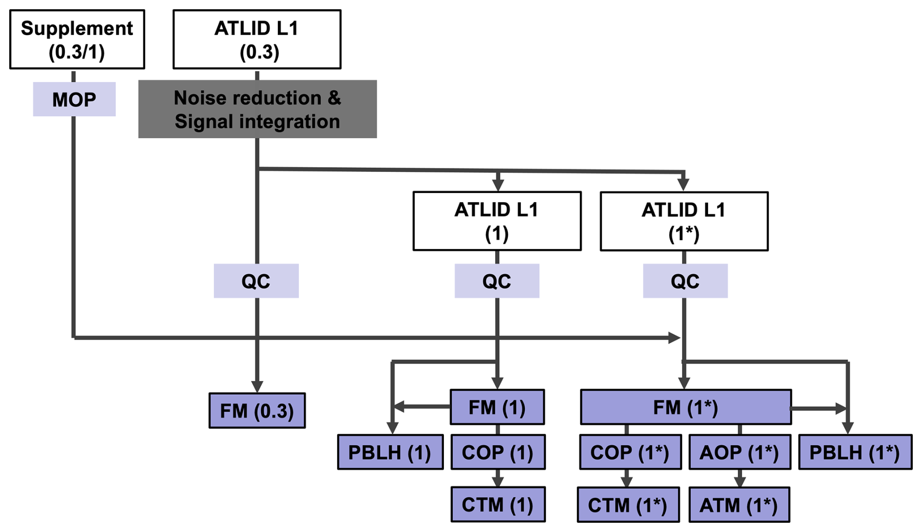
To further enhance the SNR, we integrate the data horizontally after applying the DWT method to the minimum horizontal resolution (∼0.3 km) data from ATLID L1. This integration yields data at a 1 km horizontal resolution (ATLID L1(1) in Fig. 1). Additionally, a moving average of this 1 km horizontal resolution data with a width of 10 km was produced (ATLID L1 (1*) in Fig. 1). Consequently, the algorithm uses the three L1 data created (ATLID L1 (0.3), (1), and (1*) in Fig. 1), with an altitude resolution of 0.1 km, akin to the original data, as input data when estimating each product. A quality check (QC) involving the SNR is performed on each of the generated data.

Six different products (FM (Feature Mask), AOP (Aerosol Optical Properties), COP (Cloud Optical Properties), ATM (Aerosol Target Mask), CTM (Cloud Target Mask), PBLH (Planetary Boundary Layer Height) in Fig. 1) are created from the ATLID L1 data. First, the algorithm identifies which component of atmospheric molecules, aerosols, or cloud particles is predominantly present at each altitude, and outputs its identifier (FM). Additionally, the surface, subsurface, and fully attenuated layers are identified here. Secondly, the particle optical properties (POP), that is, the extinction coefficient (α_p), backscatter coefficient (β_p), depolarization ratio (δ_p), and lidar ratio (S_p) at 355 nm, are retrieved from the ATLID L1 data. Whether the derived POP are of aerosol or cloud origin is determined according to the FM product (AOP or COP). Aerosol (ATM) and cloud (CTM) particle types are also identified at each altitude. The PBLH is then estimated. The product derived from original 0.3 km data is only the FM because of the low SNR. To account for cloud heterogeneity and the low SNR of the aerosol layers, the cloud products (COP and CTM) and PBLH are derived from the 1 km horizontal resolution data. The aerosol and cloud products (AOP, ATM, COP, and CTM) and PBLH are created from the 1* km horizontal resolution data. In the following section, products and algorithms related to aerosols (i.e., FM, AOP, ATM, PBLH) are mainly described. To estimate these products, the optical properties of atmospheric molecules, such as extinction and backscatter coefficients (MOP in Fig. 1) are required. Here, the EarthCARE auxiliary product, containing a subset of meteorological fields from an ECMWF forecast model (Eisinger et al., 2024) is used to compute the molecular optical propertes.

3 Algorithms

3.1 Layer identification (Feature mask)

The algorithm was developed based on retrieval methods developed using the CALIOP and ground-based lidar data (Okamoto et al., 2007, 2008; Hagihara et al., 2010; Shimizu et al., 2004). The algorithm classifies the atmospheric layer into molecules (clear-sky), aerosol particles, or cloud particles, as well as the surface, subsurface, and layers, where the signal is fully attenuated under optically thick layers, such as clouds (Vaughan et al., 2009). The co-polar (β_atn.M,co) and cross-polar (β_atn.M,cr) components of the Mie attenuated backscatter coefficient and Rayleigh attenuated backscatter coefficient (β_atn.R) are given as ATLID L1 products and are described by the following equations with atmospheric parameters:

$$\begin{array}{}\text{(1a)}& {\displaystyle }& {\displaystyle }{\mathit{\beta }}_{\text{atn,M,co}}={\mathit{\beta }}_{p,\text{co}}\left(z\right)\exp \left\{-\mathrm{2}\underset{z}{\overset{z_{\text{ATLID}}}{\int }}\left({\mathit{\alpha }}_p\right(z^{\prime })+{\mathit{\alpha }}_{\mathrm{m}}(z^{\prime }\left)\right)\mathrm{d}{z}^{\prime }\right\},\text{(1b)}& {\displaystyle }& {\displaystyle }{\mathit{\beta }}_{\text{atn,M,cr}}={\mathit{\beta }}_{p,\text{cr}}\left(z\right)\exp \left\{-\mathrm{2}\underset{z}{\overset{z_{\text{ATLID}}}{\int }}\left({\mathit{\alpha }}_p\right(z^{\prime })+{\mathit{\alpha }}_{\mathrm{m}}(z^{\prime }\left)\right)\mathrm{d}{z}^{\prime }\right\},\text{(1c)}& {\displaystyle }& {\displaystyle }{\mathit{\beta }}_{\text{atn,R}}={\mathit{\beta }}_{\mathrm{m}}\left(z\right)\exp \left\{-\mathrm{2}\underset{z}{\overset{z_{\text{ATLID}}}{\int }}\left({\mathit{\alpha }}_p\right(z^{\prime })+{\mathit{\alpha }}_{\mathrm{m}}(z^{\prime }\left)\right)\mathrm{d}{z}^{\prime }\right\}.\text{(1d)}& {\displaystyle }& {\displaystyle }{\mathit{\beta }}_{p,\text{co}}\left(z\right)={\mathit{\beta }}_p\left(z\right){\displaystyle \frac{\mathrm{1}}{\mathrm{1}+{\mathit{\delta }}_p\left(z\right)}},\text{(1e)}& {\displaystyle }& {\displaystyle }{\mathit{\beta }}_{p,\text{cr}}\left(z\right)={\mathit{\beta }}_p\left(z\right){\displaystyle \frac{{\mathit{\delta }}_p\left(z\right)}{\mathrm{1}+{\mathit{\delta }}_p\left(z\right)}},\text{(1f)}& {\displaystyle }& {\displaystyle }{\mathit{\beta }}_p\left(z\right)={\displaystyle \frac{{\mathit{\alpha }}_p\left(z\right)}{S_p\left(z\right)}}.\end{array}$$

where, α_p, S_p, and δ_p are the extinction coefficient, lidar ratio, and linear depolarization ratio of particles (aerosols and clouds), respectively; β_p,co and β_p,cr are the co-polar and cross-polar components of the particular backscatter coefficient, respectively; α_m and β_m are the molecular extinction coefficient and the molecular backscatter coefficient, respectively; Z is the altitude; and Z_ATLID is the altitude of ATLID. The Mie-attenuated backscatter coefficient (β_atn.M) is defined as the sum of the co-polar and cross-polar components (i.e., ${\mathit{\beta }}_{\text{atn.M}}={\mathit{\beta }}_{\text{atn.M,co}}+{\mathit{\beta }}_{\text{atn.M,cr}}$). We use β_atn,M and β_atn,R as the diagnostic parameters. The particle backscatter coefficient (${\mathit{\beta }}_p={\mathit{\beta }}_{p,\text{co}}+{\mathit{\beta }}_{p,\text{cr}}$) calculated from the following equation is also used as the diagnostic parameter :

$$\begin{array}{}\text{(2)}& {\mathit{\beta }}_{\mathrm{P}}\left(z\right)={\mathit{\beta }}_{\mathrm{m}}\left(z\right){\mathit{\beta }}_{\text{atn,M}}\left(z\right)/{\mathit{\beta }}_{\text{atn,R}}\left(z\right).\end{array}$$

First, a diagnosis is made on the 0.3 km horizontal resolution data in each layer sequentially from the upper layer to the lower layer according to the following criteria.

• (a)

  If the SNRs of β_atn,M and β_atn,R are lower than the threshold (SNR_th) or data is missing, no diagnosis is made in that layer (classified as “Invalid”).

• (b)

  If the SNR of β_atn,R is greater than the SNR_th and the SNR of β_atn,M is lower than SNR_th, the layer is classified as “Clear-sky.”

• (c)

  The SNR of β_atn,M is greather than the SNR_th, the layer is classified as “Aerosol,” “Cloud,” or “Surface.”

In this study, the value of SNR_th is set to 3.

For the layer diagnosed as “Aerosol,” “Cloud,” or “Surface,” the following further diagnoses are made. For the surface detection, the two criteria are imposed: (1) the β_atn,M is above the threshold value which is set based on actual ATLID observed data, and (2) the relevant layer is below +500 m with respect to the altitude of the Digital Elevation Model (DEM) surface altitude from the EarthCARE auxiliary data, to prevent misdetection due to clouds with large backscatter coefficieints. If the above criteria are met, the layer is marked as “Surface,” The layer below the surface is classified as “Sub-surface.”

For the cloud detection, two procedures are performed based on the cloud-mask scheme developed for the CALIOP and shipborne lidar measurements (Hagihara et al., 2010 and Okamoto et al., 2008). First, the cloud layer is detected using the following vertical variable criteria.

$$\begin{array}{}\text{(3a)}& {\displaystyle }& {\displaystyle }{\mathit{\beta }}_{\text{atn,M}}>\mathrm{0.5}{\mathit{\beta }}_{c,\text{th}}\exp (-\mathrm{2}{\mathit{\tau }}_{\mathrm{m}})\mathit{\{}\mathrm{1}-\tanh (z-z_c\left)\mathit{\right\}},\text{(3b)}& {\displaystyle }& {\displaystyle }{\mathit{\beta }}_{\mathrm{P}}>\mathrm{0.5}{\mathit{\beta }}_{c,\text{th}}\mathit{\{}\mathrm{1}-\tanh (z-z_c\left)\mathit{\right\}}\end{array}$$

where, τ_m is the molecular optical thickness up to an altitude (z) from the altitude of the ATLID. z_c is given as 5 km, and ${\mathit{\beta }}_{c,\text{th}}={\mathrm{10}}^{-\mathrm{5.25}}$ ($\sim \mathrm{5.6}\times {\mathrm{10}}^{-\mathrm{6}}$) [${\mathrm{m}}^{-\mathrm{1}}{\mathrm{sr}}^{-\mathrm{1}}$]. The validity of these threshold values was discussed in detail by Hagihara et al. (2010) and Okamoto et al. (2008). Statistical analyses of cloud and aerosol backscatter coefficient data over several years from long-term ground-based observations by HSRL (Jin et al., 2020) and Raman lidar (Nishizawa et al., 2017) also supported the value of β_c,th. If the SNR of β_atn,R of the target layer is greater than SNR_th, the Eq. (3b) is used as the criteria; otherwise, Eq. (3a), is used. The advantage of using β_P as a diagnostic parameter is that it can eliminate attenuation due to clouds/aerosols from the ATLID to the target layer. However, the calculation of the β_P requires β_atn.R in addition to β_atn.M, which has a disadvantage in that it cannot be diagnosed if the SNR of β_atn.R is insufficient. Therefore, a hybrid method is used, where β_atn.M is used if β_P cannot be used as a diagnostic parameter. After identifying the cloud layer using these critetia, a continuity test is performed to suppress misdetection due to signal noise (Hagihara et al., 2010). The continuity test is conducted on a 5-bin horizontal and 3-bin vertical window centered on the diagnostic layer, in accordance with the continuity test method used by Hagihara et al. (2010). If more than half (i.e. more than 8 bins) of the total 15 bins are clouds, the target layer is determined to be a “Cloud”. However, if the number of cloud bins was less than half of the total, but at least one of the cloud bins was included, the target layer was designated as ”Unknown.”

For 0.3 and 1 km resolution products, the “Clear-sky” or “Aerosol” layer are not diagnosed separately from the SNR's point of view, and together they are classified as “Clear-sky or aerosol” The “Fully attenuated” layer is diagnosed when no surface is detected; the layers below the lowest layer of “Clear-sky or aerosol” or “Cloud” are classified as “Fully attenuated.”

Next, a diagnosis is made on the 1 km horizontal resolution data. Diagnostics similar to those performed on the 0.3 km horizontal data are performed; the layer types of “Cloud,” “Clear-sky or aerosol,” “Surface,” “Sub-surface,” “Fully attenuated,” “Invalid,” or “Unknown” are identified. The following method is used to identify the cloud layers. The 1 km horizontal resolution data is calculated by averaging several horizontal layers (∼4 bins) of the 0.3 km horizontal resolution data. This improves the SNR, but it also causes dulling of the signal at the cloud edges, which leads to cloud layer misidentification. To suppress this, we use the FM product estimated using the 0.3 km horizontal resolution data (i.e., FM(0.3)); if more than half of the total number of the layers of the FM (0.3) product in the target layer for the 1 km horizontal resolution data is identified as “Cloud,” the target layer for the 1 km horizontal resolution data is determined to be “Cloud” (Hagihara et al., 2010). However, if the number of cloud layers is less than half of the total, but at least one of the cloud layers is included, the target layer is designated as “Unknown.” In addition, the possibility of identifying optically thin clouds or aerosols compared to the 0.3 km data, especially at high altitudes, also arises because of the improved SNR by the horizontal averaging. Equations (4a) and (4b) are then applied to the 1 km horizontal resolution data with the addition of a criterion for high altitude to Eqs. (3a) and (3b).

$$\begin{array}{}\text{(4a)}& {\displaystyle }& {\displaystyle }\begin{array}{rl}{\displaystyle }{\mathit{\beta }}_{\text{atn,M}}>& {\displaystyle }\mathrm{0.5}{\mathit{\beta }}_{c,\text{th}}\exp (-\mathrm{2}{\mathit{\tau }}_{\mathrm{m}})\mathit{\{}\mathrm{1}-\tanh (z-z_c\left)\mathit{\right\}}\\ {\displaystyle }& {\displaystyle }+\mathrm{0.5}{\mathit{\beta }}_{c,\text{th2}}\exp (-\mathrm{2}{\mathit{\tau }}_{\mathrm{m}})\mathit{\{}\mathrm{1}+\tanh (z-z_c\left)\mathit{\right\}},\end{array}\text{(4b)}& {\displaystyle }& {\displaystyle }\begin{array}{rl}{\displaystyle }{\mathit{\beta }}_{\mathrm{P}}>& {\displaystyle }\mathrm{0.5}{\mathit{\beta }}_{c,\text{th}}\mathit{\{}\mathrm{1}-\tanh (z-z_c\left)\mathit{\right\}}\\ {\displaystyle }& {\displaystyle }+\mathrm{0.5}{\mathit{\beta }}_{c,\text{th2}}\mathit{\{}\mathrm{1}+\tanh (z-z_c\left)\mathit{\right\}}\end{array}\end{array}$$

β_c,th2 is the threshold for identifying the layer that may be a cloud at high altitudes and is set based on actual ATLID data. If the criteria is satisfied, the layer is marked as “Unknown,” and if not, it is marked as Aerosol or “clear-sky” if the threshold is unsatisfied.

Finally, a diagnosis is made on the 1* km horizontal resolution data. Diagnostics similar to those performed on the 1 km horizontal resolution data are performed; the layer types of “Cloud,” “Aerosol,” “Clear-sky,” “Surface,” “Sub-surface,” “Fully attenuated,” “Invalid,” or “Unknown” are identified. Unlike the FM for the 1 km (and 0.3 km) horizontal resolution data, the layer diagnosed as “Aerosol or clear-sky” is classified into the “Aerosol” when the β_atn.M is greater than SNR_th or “Clear-sky” when the β_atn.M is lower than SNR_th.

3.2 Aerosol optical properties

As shown in Eq. (1a–c), the POP α_p, β_p, δ_p, and S_p can be directly derived using the L1 data of β_atn.M,co, β_atn.M,cr, and β_atn.R. The POP in the aerosol layer identified by the FM are classified as AOP. On the other hand, L1 data with a sufficient SN are needed to derive parameters with sufficient accuracy, especially for extinction coefficient retrieval (e.g., Liu et al., 1999). The DWT method and moving average are applied to the L1 data, but the SNR is not sufficiently large. Therefore, we simultaneously estimated the vertical profiles of the POP from the L1 data by the method of maximum likelihood with a priori smoothness constraints for the vertical profiles of the POP. The state vector x, which comprises of α_p(z_i), δ_p(z_i), and S_p(z_i) at altitudes z_i, is optimized to the L1 data by minimizing the following cost function:

$$\begin{array}{}\text{(5)}& \begin{array}{rl}{\displaystyle }& {\displaystyle }f\left(\mathit{x}\right)=\sum _i{\displaystyle \frac{{\left\{\begin{array}{l}\ln \left({\mathit{\beta }}_{\text{atn.M,co}}^{\text{obs}}\left(z_i\right)-{\mathit{\beta }}_{\text{atn.M,co}}^{\text{min}}\right)\\ -\ln \left({\mathit{\beta }}_{\text{atn.M,co}}^{\text{cal}}\left(z_i\right)-{\mathit{\beta }}_{\text{atn.M,co}}^{\text{min}}\right)\end{array}\right\}}^{\mathrm{2}}}{w_{\text{atn.M,co}}^{\mathrm{2}}\left(z_i\right)}}\\ {\displaystyle }& {\displaystyle }+\sum _i{\displaystyle \frac{{\left\{\begin{array}{l}\ln \left({\mathit{\beta }}_{\text{atn.M,cr}}^{\text{obs}}\left(z_i\right)-{\mathit{\beta }}_{\text{atn.M,cr}}^{\text{min}}\right)\\ -\ln \left({\mathit{\beta }}_{\text{atn.M,cr}}^{\text{cal}}\left(z_i\right)-{\mathit{\beta }}_{\text{atn.M,cr}}^{\text{min}}\right)\end{array}\right\}}^{\mathrm{2}}}{w_{\text{atn.M,cr}}^{\mathrm{2}}\left(z_i\right)}}\\ {\displaystyle }& {\displaystyle }+\sum _i{\displaystyle \frac{{\left\{\begin{array}{l}\ln \left({\mathit{\beta }}_{\text{atn.M,R}}^{\text{obs}}\left(z_i\right)-{\mathit{\beta }}_{\text{atn.M,R}}^{\text{min}}\right)\\ -\ln \left({\mathit{\beta }}_{\text{atn.M,R}}^{\text{cal}}\left(z_i\right)-{\mathit{\beta }}_{\text{atn.M,R}}^{\text{min}}\right)\end{array}\right\}}^{\mathrm{2}}}{w_{\text{atn.M,R}}^{\mathrm{2}}\left(z_i\right)}}\\ {\displaystyle }& {\displaystyle }+\sum _i{{\displaystyle \frac{\left\{\ln \left({\mathit{\alpha }}_p\right(z_i\left)\right)-\ln (-{\mathit{\alpha }}_p(z_{i+\mathrm{1}}\left)\right)\right\}}{w_{{\mathit{\alpha }}_P}^{\mathrm{2}}}}}^{\mathrm{2}}\\ {\displaystyle }& {\displaystyle }+\sum _i{\displaystyle \frac{{\left\{\ln \left(S_p\right(z_i\left)\right)-\ln (-S_p(z_{i+\mathrm{1}}\left)\right)\right\}}^{\mathrm{2}}}{w_{S_P}^{\mathrm{2}}}}\\ {\displaystyle }& {\displaystyle }+\sum _i{\displaystyle \frac{{\left\{\ln \left({\mathit{\delta }}_p\right(z_i\left)\right)-\ln (-{\mathit{\delta }}_p(z_{i+\mathrm{1}}\left)\right)\right\}}^{\mathrm{2}}}{w_{{\mathit{\delta }}_P}^{\mathrm{2}}}},\end{array}\end{array}$$

where z_i is ith altitude, “obs” indicates the measurements, “cal” indicates the values calculated from x by Eq. (1a–f), where z_i is ith altitude, “obs” indicates the measurements, “cal” indicates the values calculated from x by Eq. (1a–f), w_{atn.M,co/cr/R} is measurement uncertainties, $w_{{\mathit{\alpha }}_p/{\mathit{\delta }}_p/S_p}$ is weight for determine the strength of the smoothness constraint, and “min” indicates the possible minimum value of the measurements. The measurements uncertaintis w_{atn.M,co/cr/R} are calculated from the signal noises such as shot noise, dark noise, and CCD read-out noise which are evaluated befor the lauch of the EarthCARE satellite. The values of $w_{{\mathit{\alpha }}_p/{\mathit{\delta }}_p/S_p}$ are given by 1.0 in this study. A logarithmic transformation is applied to the measured and calculated values because the transformation reduces the differences of the dynamic ranges of each term in Eq. (5) and enables a fast and stable minimiation of f(x) (Kudo et al., 2016). However, the L1 data may have negative values due to large SN, and the logarithmic transformation cannot be applied to negative values. Therefore, we subtracted the possible minimum values from the measured and calculated values. The fourth, fifth, and sixth terms in Eq. (5) are the smoothness constraints for the vertical profiles of α_p(z_i), δ_p(z_i), and S_p(z_i). The smoothness of the vertical profiles is obtained by minimizing the differences of the values at two adjacent altitudes.

The minimization of f(x) is conducted by the iteration of $\ln \left({\mathit{x}}_{i+\mathrm{1}}\right)=\ln \left({\mathit{x}}_i\right)+\mathit{\gamma }\mathrm{\Delta }{\mathit{x}}_i$ in ln (x) space. The vector Δx_i at the ith step is determined by the Gauss–Newton method, and the scalar γ is determined by a line search method with Armijo rule (Nocedal and Wright, 2006). The convergence criterion for the iteration is that the difference between f(x_i) and f(x_i+1) should be smaller than a given threshold.

In the actual analysis using the ATLID data, the optical properties of clouds and aerosols are simultaneously estimated using the developed POP retrieval algorithm. To estimate the optical properties of optically thick scatterers such as clouds, it is essential to compute L1 data considering multiple scattering. The multiple scattering has been considered in CALIPSO and ground-based lidar analysis by introducing η-factor (e.g., Chen et al., 2002; Young et al., 2013; Cairo et al., 2021), and thus the η-factor will be introduced into this algorithm to estimate the optical properties of clouds. Sato et al. (2018) developed a practical model to determine the time-dependent lidar attenuated backscatter coefficient, in which an analytical expression for the high-order phase function was implemented to reduce computational cost; furthermore, Sato et al. (2019) developed a vectorized physical model (VPM) which is a physical model extended with a polarization function, to analyze the observed depolarization ratio due to multiple scattering from water clouds. The introduction of these physical models is a promising as a more advanced and accurate approach in estimating COP, considering multiple scattering from clouds.

3.3 Aerosol type classification (Target mask)

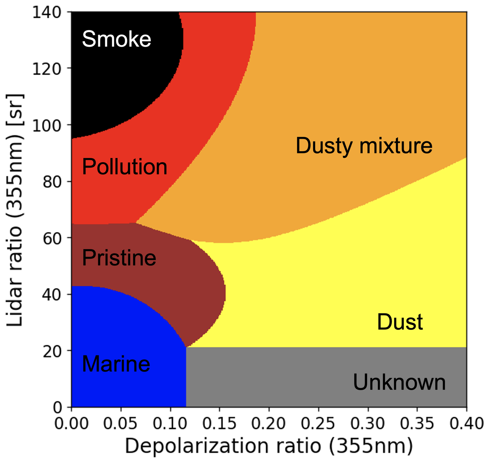
The algorithm uses the derived FM and AOP products. The algorithm classifies aerosol type for each layer that the FM scheme identifies as “Aerosol.” The algorithm uses differences in the light absorption and polarization properties of aerosol types; S_a strongly reflects the light absorption of aerosols, while δ_a strongly reflects the polarization of aerosols. Therefore, it is necessary to determine the aerosol types and their optical models. The optical properties and size distributions of aerosols are observed by the AErosol RObotic NETwork (AERONET) sun/sky photometer, and AERONET observation sites are located worldwide on all continents (e.g. Holben et al., 1998; Giles et al., 2019). In the retrieval of aerosol extinction in CALIPSO version 2 and 3 products, S_a of three aerosol types calculated by using size distributions and refractive indices of the clusters grouped by the cluster analysis of the AERONET dataset were used (Omar et al., 2005, 2009). Based on this assumption, we also perform a cluster analysis of the aerosol optical properties estimated from the AERONET data and determined the aerosol optical properties at 355 nm. In this study, aerosol particles are classified as six aerosol types (“Smoke,” “Pollution,” “Marine,” “Pristine,” “Dust,” and “Dusty mixture”) with “Unknown” in Fig. 2.

Figure 2 Lidar ratio – depolarization ratio diagram for classifying aerosol types.

The optical properties of the four aerosol types (smoke, pollution, marine, and pristine) are determined using cluster analysis of the AERONET level 2 product for years of 1992–2012. We perform a cluster analysis of the AERONET southern Africa sites for smoke type, that of Chinese sites for pollution type, and that of island sites for marine and pristine types. First, δ_a and S_a at 355, 532, and 1064 nm, which are usually observed by the HSRL and Raman lidar measurements, are calculated using the refractive indices at 440, 675, 870, and 1020 nm, size distributions of fine and coarse modes, and the sphericity of scattering light derived from the AERONET inversion algorithm (Dubovik et al., 2006) for each AERONET data sample. The refractive indices at 532 nm are interpolated and those at 355 and 1064 nm are extrapolated using those of AERONET product from 440–1020 nm. The non-spherical particle shape is assumed to be the AERONET spheroid model (Dubovik et al., 2006). Next, we adopt the fuzzy c-means method (Dunn, 1973; Bezdek, 1981) to conduct a cluster analysis. This method is based on minimizing the following objective function:

$$\begin{array}{}\text{(6)}& J=\sum _{i=\mathrm{1}}^N\sum _{k=\mathrm{1}}^K{g}_{ik}^{\mathrm{2}}\Vert x_i-c_k{\Vert }^{\mathrm{2}},\end{array}$$

where g_ik is the degree of membership of x_i to the kth cluster, x_i is the observed data, c_k is the center of the kth cluster. Partitioning is conducted through an iterative optimization of the J with updates of g_ik and c_k. Based on this cluster analysis, the center of cluster c_k is assumed to be the representative value of the selected cluster parameter. We select 12 parameters used in the cluster analysis to classify the aerosol properties. These parameters are δ_a and S_a at 355, 532, and 1064 nm and the imaginary part of the refractive index and fine mode fraction (FMF) to the total (fine + coarse) AOT at 440, 675, and 870 nm. Finally, we define the characteristic results of the cluster as the optical properties of the aerosol type.

The cluster, which is fine-mode dominated and light-absorbing aerosol, derived from the cluster analysis of the observations of AERONET sites located from 25°–35° S and 0°–40° E, which cover the source regions of African biomass burning aerosols, is assumed as the smoke type. The cluster, which is fine-mode dominated and light-absorbing aerosol, derived from the cluster analysis of the observations of AERONET sites located from 20°–40° N and 100°–125° E, which cover the source regions of Asian air pollution, is assumed as the pollution type. The marine and pristine types are derived from the cluster analysis of the observations of AERONET island sites far from aerosol source regions, where the marine type has the largest particle size with single scattering albedo (SSA) of 0.98 and the pristine type has a smaller particle size than the marine type, with the SSA of 0.98.

The difference in δ_a and S_a of non-spherical dust particles between observations and theoretical calculations remain large (Tesche et al., 2019), so that δ_a and S_a of the dust type at 355 nm are referred to as the averaged values of the Raman lidar observations in Morocco (Freudenthaler et al., 2009; Tesche et al., 2009), Germany (Wiegner et al., 2011), and Tajikistan (Hofer et al., 2017). δ_a of 0.24±0.02 and S_a of 47±8 sr for transported dust (Haarig et al., 2022) are also within the range of the dust type of the ATM. The dusty mixture type is defined as a mixture of dust and smoke in ratios of 0.65 and 0.35, respectively. Aerosol particles with high depolarization ratios and low lidar ratios are rarely observed; therefore, the unknown aerosol type is defined as aerosols with δ_a>0.12 and S_a<21 sr, which are determined by the values of the intersection of the border line between dust and pristine types and that between marine and pristine types, as shown in Fig. 2.

The ATM consists of the major tropospheric aerosol types and the optical properties of the ATM are used in the radiative transfer calculation to estimate aerosol radiative effect (Yamauchi et al., 2024). For example, volcanic ash and stratospheric aerosols, which are not included in the ATM, are misclassified as one of the aerosol types of the ATM. This misclassification is one of the uncertainties of the estimated aerosol radiative effect. However, this uncertainty is smaller than the other uncertainties in the estimation of aerosol radiative effect, because the proportions of the volcanic ash and stratospheric aerosols are considerably small in the total aerosol amounts.

In the actual analysis using ATLID data, cloud types are classified together with aerosol types. Multiple cloud particle types such as warm water, supercooled water, two-dimensional ice, and three-dimensional ice, can be identified by applying a two-dimensional diagrammatic method of signal attenuation (or extinction coefficient) and depolarization ratio developed for CALIOP cloud type classification (Yoshida et al., 2010; Okamoto et al., 2024b).

3.4 Planetary boundary layer height

We adopted the WCT method because the WCT method is less affected by noise (Qu et al., 2017), and is promising for the spaceborne lidar (Kim et al., 2021). For the PBLH detection, lidar signals at wavelength of 532 or 1064 nm are mostly used; however, the ATLID wavelength is 355 nm. Due to relatively larger Rayleigh scattering at 355 nm (approximately five times larger than that at 532 nm), the proportion of Mie scattering by aerosols in the PBL in lidar backscatter becomes relatively smaller. In other words, the difference in 355 nm backscatter signals for aerosol-rich PBL and aerosol-poor free troposphere (FT) can be smaller. The larger Rayleigh scattering at 355 nm also produces greater signal attenuation, resulting in the lower signal difference between the PBL and the FT. It should be noted that the signal attenuation due to Rayleigh scattering near the top of the PBL is generally larger for spaceborne lidar observations than for ground-based lidar observations. Thus, the detection of PBLH by spaceborne lidar observation at 355 nm is more challenging than in the past, even when the WCT method is applied (Kim et al., 2021). In this study, instead of using attenuated backscatter signals as the input of the WCT method, the backscattering ratio (BR), which can be calculated as the ratio of Mie-attenuated backscatter to Rayleigh-attenuated backscatter from the ATLID L1 data (i.e., $\text{BR}={\mathit{\beta }}_{\text{atn.M}}/{\mathit{\beta }}_{\text{atn.R}}$), is used to remove the effect of signal attenuation. Also, Rayleigh scattering component is eliminated by calculating BR minus 1 (i.e., ${\text{BR}}^{\prime }=\text{BR}-\mathrm{1}$) to highlight aerosol scattering intensity in the PBL.

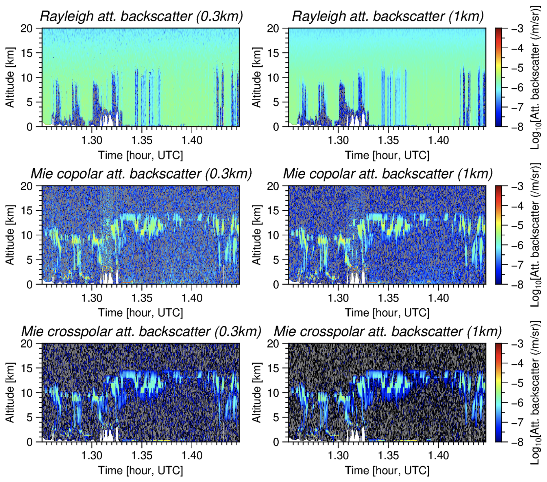
Figure 3 Rayleigh-, Mie co-polar-, and Mie cross-polar attenuated backscatter coefficients at 355 nm for cloud predominant scenes simulated using Joint-Simulator. The left/right figure shows the 0.3/1 km horizontal resolution data.

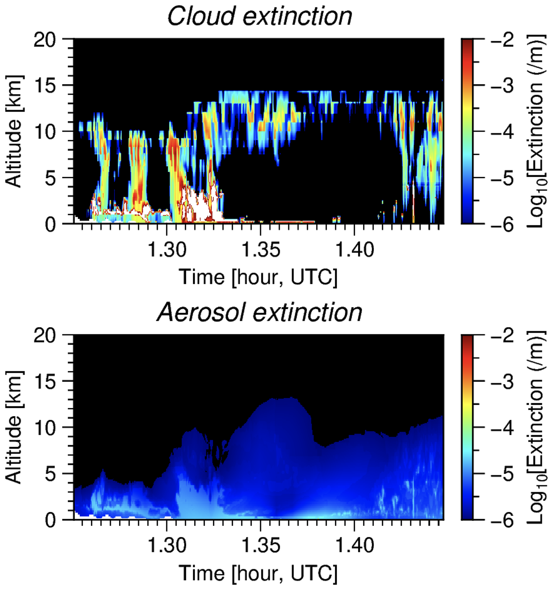
Figure 4 Extinction coefficient at 355 nm of clouds and aerosols used for the simulations for cloud predominant case (Fig. 3).

The BR^′ and FM are used as input data. Here, the target altitude (height above the surface) is set in between z_min and z_max, which are 0.1 and 5 km, respectively. If the target point is classified as a cloud in the FM at the target altitude, it is excluded from the PBLH detection. Then WCT is the calculated using the following equation:

$$\begin{array}{}\text{(7)}& \text{WCT}(a,b)={\displaystyle \frac{\mathrm{1}}{a}}\underset{z_{min}}{\overset{z_{max}}{\int }}{\text{BR}}^{\prime \left(z\right)}h\left({\displaystyle \frac{z-b}{a}}\right)\mathrm{d}z.\end{array}$$

where a and b are the dilation and the centered location of the Haar function h, which is defined as:

$$\begin{array}{}\text{(8)}& h\left({\displaystyle \frac{z-b}{a}}\right)=\left\{\begin{array}{ll}+\mathrm{1}:& b-\frac{a}{\mathrm{2}}\le z<b,\\ -\mathrm{1}:& b\le z\le b+\frac{a}{\mathrm{2}},\\ \mathrm{0}:& \text{elsewhere}.\end{array}\right.\end{array}$$

In Eq. (7), BR^′ is normalized to 1.0 for the height from the surface to 1 km to reduce the dependency of aerosol concentrations. When the WCT exceeds a threshold value, the first WCT peak from z_min is determined as the PBLH. The threshold and dilation width are determined from a simulated BR^′ profile based on ground-based HSRL data (Jin et al., 2020) with random noise according to the errors in the ATLID attenuated backscatter reported by do Carmo et al. (2021), and are set to 0.2 and 1.0 km, respectively.

4 Results and Discussion

To demonstrate the products and the performance of the algorithms, the ATLID L1 data (i.e., Eq. 1a–c) simulated using the Joint Simulator for Satellite Sensors (Joint-Simulator) (Hashino et al., 2013, Satoh et al., 2016, Roh et al., 2023a) were used. Cloud (and precipitation) distributions simulated using the Nonhydorstatic Icosahedral Atmospheric Model (NICAM; Satoh et al., 2014) and aerosol distributions simulated using NICAM Spectral Radiation Transport Model for Aerosol Species (NICAM-SPRINTARS; Takemura et al., 2000) were used as the input data. Signal noises such as shot noise, dark noise, and CCD read-out noise expected from the ATLID system were evaluated and added as gaussian random noise.

The ATLID L1 data for the cloud-predominant case simulated along the satellite path using Joint-Simulator are shown in Fig. 3. The cloud and aerosol fields used for the signal simulation are also shown in Fig. 4. Clouds are present from the surface to the altitude of 15 km. The SNR of the Mie co-polar- and cross-polar attenuated backscatter coefficients for the cloud layers are generally greater than 5 for 0.3 km horizontal resolution data; the SNR for 1 km horizontal resolution data is approximately twice than that for 0.3 km horizontal resolution data. The FM algorithm (Sect. 3.1) was applied to the simulated L1 data (Fig. 5). To assess the effect of signal noise on the estimates, the algorithm was applied to L1 data with or without signal noise, and the agreement between them was evaluated. The results for the 0.3 and 1 km horizontal resolution data showed generally good agreement for each layer type, such as “cloud” and “clear-sky or aerosol.” For the 0.3 km horizontal resolution data, the total number of layers for the cloud type was 226 000, of which the number of misidentification was 24 000, corresponding to a 11 % relative error. For the 1 km horizontal resolution data, the misidentification of the cloud layers was 9 %. For the clear-sky or aerosol type, the misidentification reached to 41 % for the 0.3 km horizontal resolution data; however, it improved to 5 % for the 1 km horizontal resolution data. Many misidentification were noted at the edges of the cloud layers, highlighting the need for improvement is this aspect in future studies.

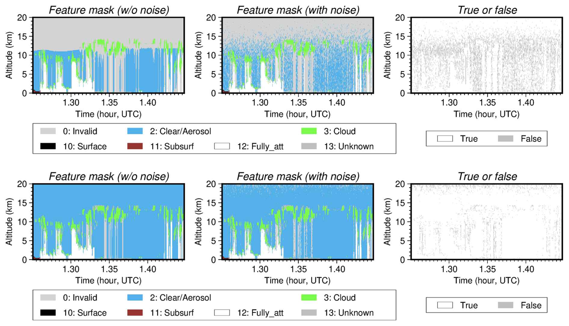
Figure 5 Feature mask products estimated for data with/without signal noise for cloud predominant scenes (Fig. 3) and its true or false values. The upper/lower figures show the results for the 0.3/1 km horizontal resolution data.

The results of the aerosol layer identification are shown in Fig. 7. Here, we used the the L1 data simulated for the aerosol-predominant case, where the dust layer is widely suspended over an altitude range of 3–20 km (Fig. 6), and the FM algorithm was applied to the L1 data with or without noise. The results for the data with signal noise are generally in good agreement with those for the data without signal noise. The total number of aerosol layers was approximately 280 000 and the number of misidentified layers was 30 000, resulting in 11 % misidentification. As in the cloud-predominant case (Fig. 5), much of the misidentification occurred at the edges of the aerosol layers, which is also an aspect that can be improved for aerosol identification.

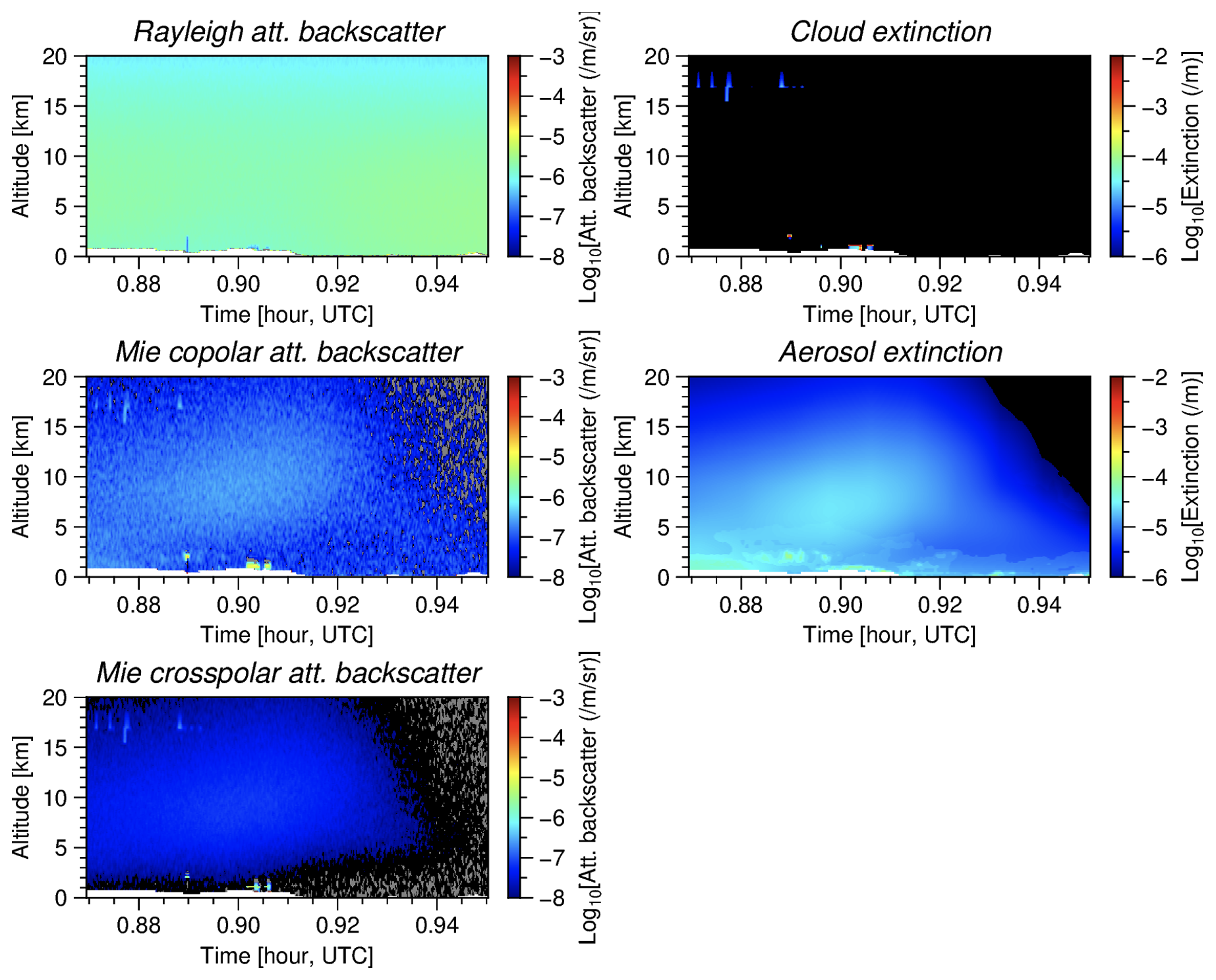
Figure 6 Rayleigh-, Mie co-polar-, and Mie cross-polar attenuated backscatter coefficients at 355 nm for aerosol predominant scenes simulated using Joint-Simulator and extinction coefficients at 355 nm of aerosols and clouds. The simulations shown used 1* km horizontal resolution data.

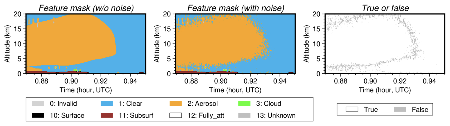
Figure 7 Feature mask products estimated for data with/without signal noise for aerosol predominant cases (Fig. 6) and its true or false values.

The results of the AOP retrieval are shown in Fig. 8. The AOP retrieval algorithm was applied to the aerosol-predominant case, as shown in Fig. 6. The SNRs of the L1 data for the dust layer generally ranged from 5–20 for 1* km horizontal resolution data. The estimated backscatter coefficients and depolarization ratios generally agreed well with the actual values, which were the aerosol optical properties used in the L1 simulation. The mean of retrieved aerosol backscatter coefficient was $\mathrm{3.26}\times {\mathrm{10}}^{-\mathrm{7}}{\mathrm{m}}^{-\mathrm{1}}{\mathrm{sr}}^{-\mathrm{1}}$. The true value was $\mathrm{3.18}\times {\mathrm{10}}^{-\mathrm{7}}{\mathrm{m}}^{-\mathrm{1}}{\mathrm{sr}}^{-\mathrm{1}}$ and the mean error (ME: retrieval–truth) was $\mathrm{0.08}\times {\mathrm{10}}^{-\mathrm{7}}{\mathrm{m}}^{-\mathrm{1}}{\mathrm{sr}}^{-\mathrm{1}}$, corresponding to a relative error of 2 %. The root mean square error (RMSE) was $\mathrm{1.12}\times {\mathrm{10}}^{-\mathrm{7}}{\mathrm{m}}^{-\mathrm{1}}{\mathrm{sr}}^{-\mathrm{1}}$, corresponding to a relative error of 34 %. For the depolarization ratio, the means for the retrievals and true values were 0.27 and 0.26, respectively; ME=0.01 (4 %) and RMSE=0.07 (27 %). The figure also shows that the extinction coefficient and lidar ratio were more strongly affected by the signal noise than the backscatter coefficient and depolarization ratio. For the extinction coefficient, the means for the retrieval and true values were $\mathrm{1.32}\times {\mathrm{10}}^{-\mathrm{5}}$ and $\mathrm{1.35}\times {\mathrm{10}}^{-\mathrm{5}}{\mathrm{m}}^{-\mathrm{1}}$, respectively; $\text{ME}=-\mathrm{0.03}{\mathrm{m}}^{-\mathrm{1}}$ (2 %) and $\text{RMSE}=\mathrm{1.05}\times {\mathrm{10}}^{-\mathrm{5}}{\mathrm{m}}^{-\mathrm{1}}$ (78 %). For the lidar ratio, the means of the retrieval and true values were 41 sr⁻¹, respectively; $\text{ME}=\mathrm{0}{\mathrm{sr}}^{-\mathrm{1}}$ (0 %) and $\text{RMSE}=\mathrm{25}{\mathrm{sr}}^{-\mathrm{1}}$ (61 %). As with the backscatter coefficient and depolarization ratio, there was no significant bias error (ME) for the extinction coefficient and lidar ratio; however, the variation (RMSE) was relatively large owing to signal noise. Notably, the aerosol concentration used in this analysis was relatively low (i.e., $\mathrm{1.35}\times {\mathrm{10}}^{-\mathrm{5}}{\mathrm{m}}^{-\mathrm{1}}$ on an average), and the RMSE value of the extinction coefficient is not large (i.e., $\mathrm{1.05}\times {\mathrm{10}}^{-\mathrm{5}}{\mathrm{m}}^{-\mathrm{1}}$). For cases with higher aerosol concentrations, it can be expected that the relative error of the extinction coefficient and the RMSE of the lidar ratio decrease with an increase in the SNR of the Mie-attenuated backscatter coefficient (e.g., Nishizawa et al., 2017).

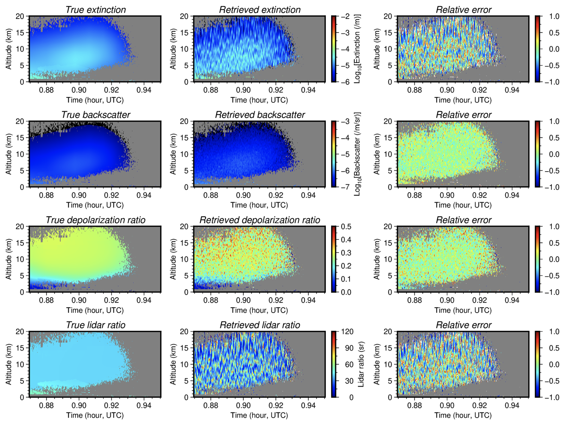
Figure 8 Extinction coefficient, backscatter coefficient, depolarization ratio, and lidar ratio of aerosols estimated for aerosol predominant cases (Fig. 6) and its relative error.

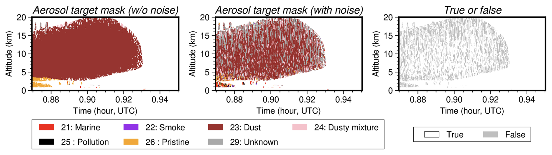
Figure 9 Aerosol target mask products estimated for data with/without signal noise for aerosol predominant scenes (Fig. 6) and its true or false values.

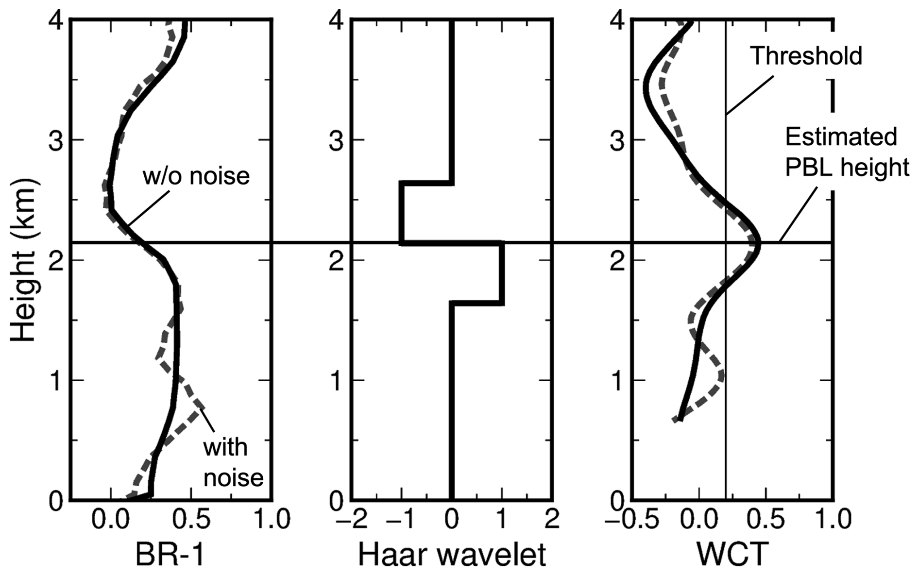
Figure 10 Vertical profiles of (left) backscattering ratio (BR) minus 1 for the simulated ATLID L1 data, (center) Haar function, and (right) wavelet covariance transform (WCT).

The results of the aerosol-type classification are shown in Fig. 9. The algorithm was applied to the L1 data with and without signal noise for the aerosol-predominant case, as shown in Fig. 6. For the dust layer, there appeared some misclassification (e.g., Dusty-mixture and Unknown); however, there was a fair amount of agreement. The total number of layers classified as Dust type was approximately 225 000 and the number of misidentified layers was 84 000, resulting in a 37 % misidentification. In addition, aerosol layers classified as Pristine type were also found below an altitude of 4 km; the total number of pristine layers was approximately 13 000 and the number of misidentified layers was 9700, resulting in 74 % misidentification. Since aerosol typing was classified using a two-dimensional diagram of the lidar and depolarization ratios (Fig. 2), aerosol type misclassification is directly reflected by the errors in the lidar ratio and depolarization ratio. The error in the lidar ratio is considerably larger than that in the depolarization ratio (about 25 sr in RMSE). Therefore, the retrieved lidar ratios for the dust layer fall outside the range of the two-dimensional diagram for “dust”, resulting in cases of misclassification as dusty-mixture or unknown. Similarly, pristine is misclassified as pollution or marine due to the errors in the lidar ratio. Thus, accurate estimation of the lidar ratio as well as depolarization ratio is required for aerosol type classification. For cases with higher aerosol concentrations, it can be expected that the misclassification of aerosol types decreases with an decrease of the retrieval error of the lidar ratio, as discussed in the AOP retrieval (Sect. 4).

Figure 10 shows an example of the PBLH detection for the L1 data simulated using Joint-Simulator, where the PBLH was approximately 2.1 km. The WCT was calculated using a Haar function with a dilation width of 1.0 km, and a WCT peak exceeding a threshold of 0.2, derived at 2.1 km. When signal noise was added to the L1 data (dotted line in Fig. 10), another WCT peak at ∼1 km appeared because of signal fluctuation; however, the peak was below the threshold. In this case, the estimated PBLH with noise agreed well with that without noise. In actual observations, the PBLH detection may be difficult for cases of noisy data, low aerosol concentrations, and the existence of residual layers at night because the gap of BR^′ for the PBL and free troposphere may be small.

5 Conclusion

We developed algorithms to produce JAXA ATLID L2 products for aerosols and clouds using ATLID L1 data. The algorithms retrieve the following products: (1) feature mask; (2) particle optical properties such as extinction coefficient, backscatter coefficient, depolarization ratio, and lidar ratio at 355 nm; (3) target mask; and (4) planetary boundary layer height. The performance of the algorithms was demonstrated using pseudo-ATLID L1 data with realistic signal noise, which were calculated according to the ATLID specification for the aerosol or cloud dominated cases by Joint-Simulator.

The main findings of this simulation study are as follows: (1) the misidentification of the aerosol and cloud layers by the feature mask algorithm was relatively low (approximately 10 %). (2) The retrieval errors of the AOP were $\mathrm{0.08}\times {\mathrm{10}}^{-\mathrm{7}}\pm \mathrm{1.12}\times {\mathrm{10}}^{-\mathrm{7}}{\mathrm{m}}^{-\mathrm{1}}{\mathrm{sr}}^{-\mathrm{1}}$ (2±34 % relative error) for the backscatter coefficient and 0.01±0.07 (4±27 % relative error) for the depolarization ratio of aerosols; the relative errors of the extinction coefficient and lidar ratio were worse than those of the backscatter coefficient and depolarization ratio. (3) The aerosol-type classification generally performed well, with 37 % misclassifications for the dust type, although there were more misclassifications for the pristine type. These misidentifications were mainly due to errors in the estimation of the lidar ratios. Accurate estimation of the lidar ratio as well as depolarization ratio is essential for aerosol type classification. (4) PBLH retrieval using the WCT method with ATLID L1 data was feasible. These results indicate that the algorithm's capability to provide valuable insights into the global distribution of aerosols and clouds, facilitating assessments of their climate impact through atmospheric radiation processes.

The validation of these aerosol and cloud products is essential, and JAXA and ESA will conduct validation using various platforms, such as airborne, shipborne, and ground-based measurements, and various observation instruments, including lidars. The validation studies include assuarance of the product accuracy and the improvement of the L2 algorithms mentioned above, including the verification and improvement of various assumptions (e.g., optical models of aerosols and clouds) and the criteria used in the algorithms.

To understand the climatic effects of aerosols, it is essential to understand the properties of individual aerosol components as well as the properties of total aerosols such as the JAXA ATLID L2 products described above. Therefore, we are currently developing an algorithm to estimate the extinction coefficients of dust, sea salt, carbonaceous (light-absorbing particles), and water-soluble aerosols at 355 nm using the difference in the depolarization and light absorption properties of each aerosol component from the L2 products and ATLID L1 data. We are also currently developing an ATLID-MSI synergy algorithm to retrieve the vertical mean mode-radii of dust and fine-mode aerosols, and the extinction coefficients of the abovementioned four aerosol components. These algorithms are being developed based on the aerosol component retrieval algorithms that have been developed for the analysis of CALIOP and ground-based lidar data. (Kudo et al., 2023; Nishizawa et al., 2007, 2008, 2011, 2017). The aerosol component products derived by these algorithms using ATLID and MSI data are planned to be released as JAXA's L2 products and are expected to enhance the scientific value of the EarthCARE mission.