Seeking TOA SW flux closure over semi-synthetic 3D cloud fields: exploring the accuracy of two angular distribution models

To accurately estimate outgoing top-of-atmosphere (TOA) shortwave (SW) fluxes from measurements of broadband radiances, angular distribution models (ADMs) are necessary. ADMs rely on radiance-predicting models that are trained on hemispherically-resolved CERES TOA radiance observations. The estimation of SW fluxes is particularly challenging for cloudy skies due to clouds' anisotropy, which substantially varies with their optical properties for any given sun-object-observer geometry. The aim of this study is to investigate the influence of micro- and macrophysical properties of liquid clouds on SW fluxes estimated by ADMs that are based on a semi-physical model and compare to operational ADMs. We hypothesize that a microphysically aware ADM performs better in observation angles influenced by single-scattering features.

The semi-physical approach relies on a parameterized asymmetry parameter g^Δ, which depends on the cloud effective radius and, after adjustments during training of the model, explicitly varies with sun–observer geometry. We link these adjustments to single scattering features, such as the shift of the cloud bow and glory with varying cloud droplet sizes.

For the investigation, 125 3D cloud scenes are constructed based on observational data and theoretical assumptions. Using a Monte Carlo model, the TOA broadband SW radiances and fluxes of the semi-synthetic cloud scenes are simulated for different scenarios with varying viewing angles (θ_v) along the principal plane and solar angles (θ_s). Based on the resulting 20 000 scenarios, the sensitivity and accuracy of the two SW radiance-to-irradiance conversion approaches to cloud droplet size, spatial distribution of liquid water path, and mean optical thickness are quantified.

The study emphasizes that explicitly including the liquid droplet effective radius in ADM generation can improve the accuracy of shortwave flux estimates. Particularly for viewing geometries that exhibit single scattering phenomena, such as cloud glory and cloud bow, flux estimates can benefit from microphysically aware ADMs. For the analyzed scenarios, we found that the errors of instantaneous TOA SW flux estimates could be reduced by up to 25 W m⁻². For scenes with very large or small droplets, the median error was reduced by up to 7 W m⁻².

1 Introduction

The Earth radiation budget (ERB) quantifies the overall balance of incoming solar radiation and outgoing reflected solar and emitted thermal radiation at the top of the atmosphere (TOA). Quantifying ERB is fundamental for understanding how the climate of Earth will change in the future. The main parameters influencing the ERB are the Earth's surface, clouds, aerosols, and atmospheric gases (e.g. Loeb and Manalo-Smith, 2005; Wild et al., 2014, 2018; Forster et al., 2021). TOA outgoing radiative fluxes are estimated using, e.g., radiance measurements of broadband (BB) radiometers aboard polar orbiting and geostationary satellites (e.g. Viollier et al., 2009; Dewitte et al., 2008; Velázquez Blázquez et al., 2024a).

However, accurately estimating the flux leaving Earth's TOA using only one measurement at a single sun-observer geometry, as is the case for satellites, is challenging. In particular, the reflected solar radiation can be highly anisotropic, depending on the observed scene. For clouds, the dependency on sun–observer geometry is complex and governed by their macro- and microphysical properties. Over the past decades, a variety of radiance-predicting models have been developed and refined to estimate the anisotropy of observed cloud scenes (e.g., Smith et al., 1986; Loeb et al., 2003, 2005; Su et al., 2015; Domenech and Wehr, 2011; Tornow et al., 2021; Velázquez Blázquez et al., 2024b). Using these distribution models (ADMs) the radiance-to-irradiance (flux) conversion can be achieved from a single satellite observation. An overview of different SW ADM approaches is given in Gristey et al. (2021).

In this study, we investigate TOA SW flux estimates for overcast marine liquid cloud scenes with varying macro- and microphysical properties. SW fluxes are estimated using two sets of ADMs: one based on the semi-physical log-linear model (Tornow et al., 2020, 2021) (semi-physical approach), and a second set derived using the state-of-the art sigmoidal approach (Su et al., 2015). The later is the currently operational approach used for SW flux estimates above clouds, for example, by the Clouds and the Earth's Radiant Energy System (CERES). The flux estimates from CERES are the input for the ANN (Artificial Neural Network) approach, used in the EarthCARE BMA-FLX processor (Velázquez Blázquez et al., 2024b). To analyze the accuracy of the SW flux estimates and the sensitivity to micro- and macrophysical properties, we use 125 different semi-synthetic 3D cloud scenes to simulate TOA radiances and fluxes using a Monte Carlo model. The semi-physical approach explicitly incorporates the mean cloud top effective radius (${\stackrel{\mathrm{‾}}{r}}_{\mathrm{eff}}^{\mathrm{ctop}}$) via the parameterized asymmetry parameter (g^Δ; Tornow et al., 2020), which also depends on the sun-observer angular-bin (^Δ). The study addresses the following main research questions:

1. How sensitive is the accuracy of TOA SW flux estimates to variations in effective radius, cloud homogeneity and optical thickness?

2. Can the explicit incorporation of cloud microphysics in a radiance-to-irradiance conversion approach improve the accuracy of SW flux estimates?

3. Are the adjustments of the asymmetry parameter g^Δ resulting from the optimization process physically plausible, and what are the underlying causes for this?

Section 2 describes the theoretical basis of ADMs, the generation of 3D cloud scenes, and the configuration of the Monte Carlo model. In Sect. 3, the results are discussed, and in Sect. 4, the findings are summarized and concluded.

2 Theoretical Basis and Methodology

ADMs describe the hemispherically resolved deviation of TOA angular-bin mean radiance $\stackrel{\mathrm{‾}}{I}({\mathit{\theta }}_{\mathrm{s}},{\mathit{\theta }}_{\mathrm{v}},\mathit{\varphi })$ from the isotropic case. The deviation is expressed through the anisotropic factor (R), where values greater than one indicate stronger reflection than the isotropic case, and values less than one indicate weaker reflection. Equation (1) describes how the anisotropic factor for a given solar zenith θ_s, viewing zenith θ_v, and relative azimuth angle ϕ is calculated.

$$\begin{array}{}\text{(1)}& {\displaystyle }R\left({\mathit{\theta }}_{\mathrm{s}},{\mathit{\theta }}_{\mathrm{v}},\mathit{\varphi }\right)={\displaystyle \frac{\mathit{\pi }\stackrel{\mathrm{‾}}{I}\left({\mathit{\theta }}_{\mathrm{s}},{\mathit{\theta }}_{\mathrm{v}},\mathit{\varphi }\right)}{{\int }_{\mathrm{0}}^{\mathrm{2}\mathit{\pi }}{\int }_{\mathrm{0}}^{\mathit{\pi }/\mathrm{2}}\stackrel{\mathrm{‾}}{I}\left({\mathit{\theta }}_{\mathrm{s}},{\mathit{\theta }}_{\mathrm{v}},\mathit{\varphi }\right)\cos {\mathit{\theta }}_{\mathrm{v}}\sin {\mathit{\theta }}_{\mathrm{v}}\mathrm{d}{\mathit{\theta }}_{\mathrm{v}}\mathrm{d}\mathit{\varphi }}}\text{(2)}& {\displaystyle }={\displaystyle \frac{\mathit{\pi }\stackrel{\mathrm{‾}}{I}\left({\mathit{\theta }}_{\mathrm{s}},{\mathit{\theta }}_{\mathrm{v}},\mathit{\varphi }\right)}{\stackrel{\mathrm{‾}}{F}\left({\mathit{\theta }}_{\mathrm{s}}\right)}}\end{array}$$

For a radiance observation I_o at a given sun-observer geometry, the TOA flux estimates (F(θ_s)) are calculated using the anisotropic factor derived in Eq. (1), following Eq. (3).

$$\begin{array}{}\text{(3)}& F\left({\mathit{\theta }}_{\mathrm{s}}\right)={\displaystyle \frac{\mathit{\pi }{I}_{\mathrm{o}}\left({\mathit{\theta }}_{\mathrm{s}},{\mathit{\theta }}_{\mathrm{v}},\mathit{\varphi }\right)}{R\left({\mathit{\theta }}_{\mathrm{s}},{\mathit{\theta }}_{\mathrm{v}},\mathit{\varphi }\right)}}\end{array}$$

2.1 Sigmoidal approach

The currently operational approach to construct ADMs over marine clouds is described in, e.g., Su et al. (2015) and is an extension of the approach from Loeb et al. (2005). For the approach, information of the CERES footprint average cloud optical depth $\stackrel{\mathrm{‾}}{\mathit{\tau }}$ (exponential of the average over logarithmic τ values) and the cloud fraction f (in %) is used to predict the hemispherical field of TOA SW radiances $\stackrel{\mathrm{‾}}{I}$. Per angular-bin a sigmoidal function (Eq. 4) is fitted to the observed CERES radiance I and x = $\log \left(f\cdot \stackrel{\mathrm{‾}}{\mathit{\tau }}\right)$. Where solar irradiance I₀ as well as a, b, c, and x₀ are free parameters in the model.

$$\begin{array}{}\text{(4)}& I=I_{\mathrm{0}}+{\displaystyle \frac{a}{{\left[\mathrm{1}+e^{-(x-x_{\mathrm{0}})/b}\right]}^c}}\end{array}$$

2.2 Semi-physical approach

As for the sigmoidal approach, the semi-physical approach uses CERES footprint average cloud optical depth $\stackrel{\mathrm{‾}}{\mathit{\tau }}$ and the cloud fraction f (here not in % but as fraction). Additionally, the semi-physical approach includes information of the cloud microphysics in the form of the footprint averaged effective radius (${\stackrel{\mathrm{‾}}{r}}_{\mathrm{eff}}^{\mathrm{ctop}}$) explicitly. Furthermore, the water vapor load above the clouds (above cloud water vapor, ACWV) is taken into account.

In Tornow et al. (2018) the TOA SW anisotropy has been found to be sensitive to both ${\stackrel{\mathrm{‾}}{r}}_{\mathrm{eff}}^{\mathrm{ctop}}$ and ACWV. In the case of effective radius, anisotropy differences of up to 8 % were found. To incorporate these dependencies, a simple model (Eq. 5) relating the outgoing radiance I, to the incoming solar irradiance (I₀) via a footprint albedo α and a factor describing the attenuation due to water vapor above clouds (e^−2ACWV) has been formulated. The factor 2 arises from the fact that the light passes the water vapor layer twice before reaching the TOA. By using the logarithm (Eq. 6) the model becomes linear and a simple first-degree polynomial function (Eq. 9) can be fitted to the observations.

$$\begin{array}{}\text{(5)}& {\displaystyle }I\left({\mathit{\theta }}_{\mathrm{s}},{\mathit{\theta }}_{\mathrm{v}},\mathit{\varphi }\right)\sim I_{\mathrm{0}}\cdot \mathit{\alpha }\cdot e^{-\mathrm{2}\cdot \mathrm{ACWV}}\text{(6)}& {\displaystyle }\log I\left({\mathit{\theta }}_{\mathrm{s}},{\mathit{\theta }}_{\mathrm{v}},\mathit{\varphi }\right)\sim \log I_{\mathrm{0}}+\log \mathit{\alpha }-\mathrm{2}\cdot \text{ACWV}\end{array}$$

The footprint albedo α (Eq. 7) is the sum of the clear sky portion of the scene (f₀) multiplied with the clear sky albedo (α^cs) and the cloud fraction (f₁) multiplied with the two-stream albedo (α_ts, Eq. 8). α_ts is the Coakley–Chylek approximation (Coakley and Chylek, 1975) and depends on the footprint mean cloud optical thickness ($\stackrel{\mathrm{‾}}{\mathit{\tau }}$) and the parameterized asymmetry parameter (g^Δ) for the given sun-observer bin ^Δ.

$$\begin{array}{}\text{(7)}& {\displaystyle }\mathit{\alpha }=f_{\mathrm{0}}\cdot {\mathit{\alpha }}_{\mathrm{cs}}+f_{\mathrm{1}}\cdot {\mathit{\alpha }}_{\mathrm{ts}}\text{(8)}& {\displaystyle }{\mathit{\alpha }}_{\mathrm{ts}}={\displaystyle \frac{(\mathrm{1}-g^{\mathrm{\Delta }}\left({\stackrel{\mathrm{‾}}{r}}_{\mathrm{eff}}^{\mathrm{ctop}}\right))\cdot \stackrel{\mathrm{‾}}{\mathit{\tau }}/\mathrm{2}}{\mathrm{1}+\left(\mathrm{1}-g^{\mathrm{\Delta }}\left({\stackrel{\mathrm{‾}}{r}}_{\mathrm{eff}}^{\mathrm{ctop}}\right)\right)\cdot \stackrel{\mathrm{‾}}{\mathit{\tau }}/\mathrm{2}}}\end{array}$$

Parameterized asymmetry parameter

The asymmetry parameter g in the two-stream albedo describes the tendency of radiation to scatter in the forward or backward direction. Symmetric scattering corresponds to g = 0, positive values (g > 0) to stronger forward scattering, and negative values (g < 0) to stronger backward scattering. g is a function of cloud microphysics, represented in this study by the footprint-mean cloud-top effective radius (${\stackrel{\mathrm{‾}}{r}}_{\mathrm{eff}}^{\mathrm{ctop}}$), and is for marine liquid clouds about 0.86. In the semi-physical approach, g is optimized during model training for each sun–observer geometry bin (Δ) to reduce residuals between the MODIS observations and the model (Tornow et al., 2020). Due to this bin-wise optimization, the parameterized $g^{\mathrm{\Delta }}\left({\stackrel{\mathrm{‾}}{r}}_{\mathrm{eff}}^{\mathrm{ctop}}\right)$ now also depends on the angular-bin Δ (see, e.g., Fig. 7, lower panel). This optimization implicitly accounts for various 3D effects, as well as single-scattering features related to the underlying phase function, such as the broadening and forward shift of the cloud glory, and the shift of the cloud bow toward the backscatter direction for smaller ${\stackrel{\mathrm{‾}}{r}}_{\mathrm{eff}}^{\mathrm{ctop}}$ (e.g., Mayer et al., 2004). With this new dependency, these single-scattering features become apparent in the radiances modeled using the semi-physical approach (see, e.g., Figs. 1 and 6).

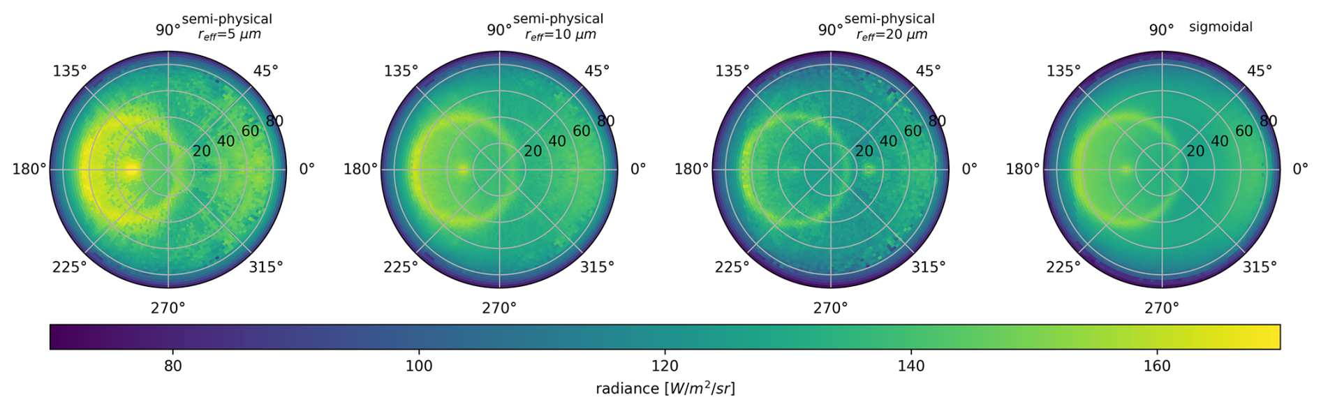
Figure 1 Radiance ($\stackrel{\mathrm{‾}}{I}$) predicted for a θ_s of 27° and an overcast scene over ocean with $\stackrel{\mathrm{‾}}{\mathit{\tau }}$ = 10. The three panels on the left show simulations using the semi-physical approach with variable r_eff and the right panel using the sigmoidal approach.

The semi-physical model is fitted to the observations using an ordinary-least-square method with the free parameters A, B, C (Eq. 9).

$$\begin{array}{}\text{(9)}& \log I\left({\mathit{\theta }}_{\mathrm{s}}^{\mathrm{\Delta }},{\mathit{\theta }}_{\mathrm{v}}^{\mathrm{\Delta }},{\mathit{\varphi }}^{\mathrm{\Delta }}\right)\approx \text{A}+\text{B}\cdot \log \mathit{\alpha }+\text{C}\cdot \text{ACWV}\end{array}$$

Throughout this study, only overcast ocean scenes (f₁ = 1) with a clear-sky fraction set to zero (f₀ = 0) and no above cloud water vapor (ACWV = 0) are considered.

Figure 1 shows the predicted radiances using ADMs based on the sigmoidal approach (right panel) and on the semi-physical approach with varying ${\stackrel{\mathrm{‾}}{r}}_{\mathrm{eff}}^{\mathrm{ctop}}$ (three left panels) and illustrates the sensitivity of the semi-physical approach to cloud microphysics. In the figure, both approaches agree best for a ${\stackrel{\mathrm{‾}}{r}}_{\mathrm{eff}}^{\mathrm{ctop}}$ of 10 µm, which is in the range of average values found in marine boundary layer stratocumulus clouds. For decreasing ${\stackrel{\mathrm{‾}}{r}}_{\mathrm{eff}}^{\mathrm{ctop}}$ the broadening of cloud glory and bow becomes apparent.

A detailed explanation and further discussion of the semi-physical approach can be found in Tornow et al. (2018, 2020, 2021).

For the creation of both sets of ADMs, the same CERES Ed4SSF (Edition 4.0 Single Scanner Footprint) observations between 2000 and 2005 have been used. In this period, CERES aboard Aqua and Terra measured in the rotating azimuth plane scan mode, providing angular coverage for the ADM construction. The CERES Ed4SSF dataset of Aqua and Terra (described in Su et al., 2015) combines MODIS and CERES L2 data. The observations were grouped into sun–observer bins (^Δ) spanning a 2° × 2° hemispherical grid. Only observations with more than 95 % water surface, more than 0.1 % cloud fraction, and solar zenith angles between 0 and 82° have been used. In the case of $\ln \left(\stackrel{\mathrm{‾}}{\mathit{\tau }}f\right)$ < 6 (where f is in %) a look-up table approach has been used instead of sigmoidal fit in sun glint affected geometries (sun glint angle < 20°). Further explanation on the selection of data and the methodology to fit the two approaches can be found in Tornow et al. (2021). By using two extra retrieved parameters (r_eff and ACWV), the semi-physical approach is affected by additional retrieval uncertainties.

To explore the research questions raised above, 125 semi-synthetical 30 × 30 km² 3D-cloud scenes with a horizontal resolution of 1 km and varying mean optical thicknesses ($\stackrel{\mathrm{‾}}{\mathit{\tau }}$), homogeneities (ν) and droplet number concentrations (N_d) are generated. The scenes are based on MODIS observations, and the vertical dimension is added using cloud adiabatic theory. The exact procedure is explained below.

2.3 Brief Recap on Cloud Adiabatic Theory

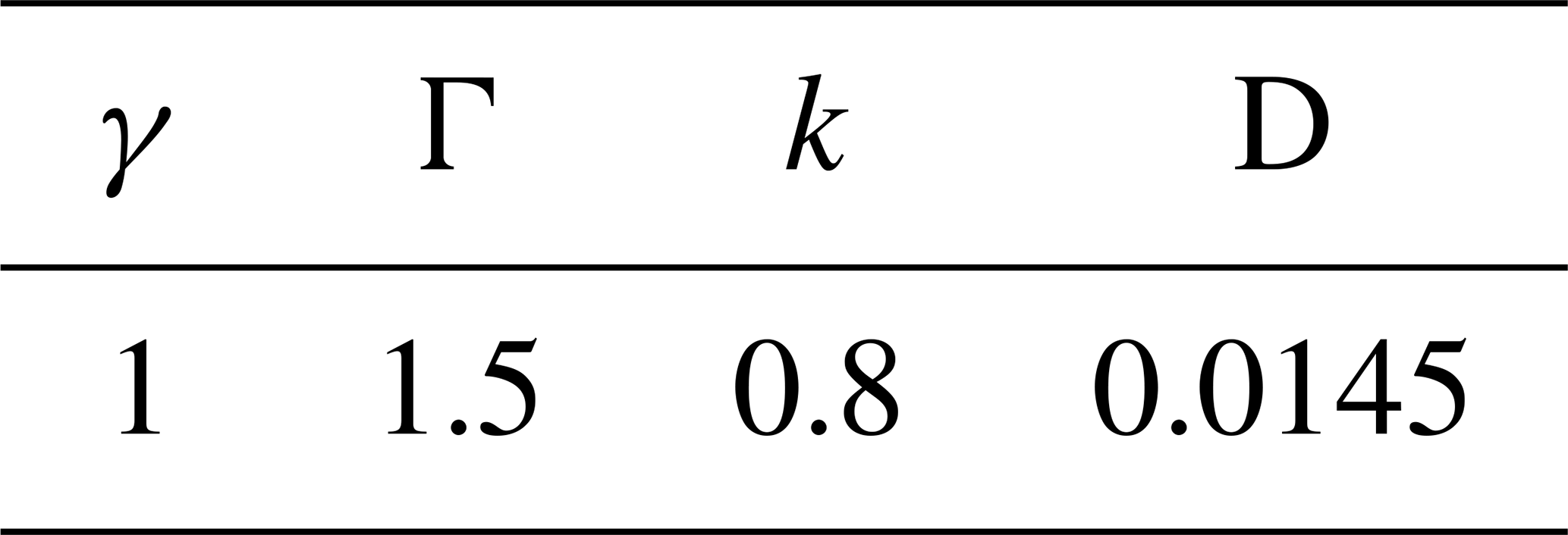
Following the adiabatic theory described, for example, in Brenguier et al. (2000) and Wood (2006), the vertical profile of cloud liquid water content (LWC) can be approximated by Eq. (10). The mean cloud volume radius (r_vol) for a given layer depends on the amount of liquid water in the layer LWC and the concentration of cloud droplets (N_d). The effective radius (r_eff) is related to r_vol via the constant k (see Eq. 12).

$$\begin{array}{}\text{(10)}& {\displaystyle }\mathrm{\text{LWC}}\left(z\right)=\mathit{\gamma }\cdot \mathrm{\Gamma }\cdot z\text{(11)}& {\displaystyle }{r}_{\mathrm{vol}}=({\displaystyle \frac{\mathrm{3}\text{LWC}}{\mathrm{4}\mathit{\pi }{\mathit{\rho }}_{\mathrm{w}}{N}_{\mathrm{d}}}}{)}^{\mathrm{1}/\mathrm{3}}\text{(12)}& {\displaystyle }{r}_{\mathrm{eff}}=k^{-\mathrm{1}/\mathrm{3}}\cdot r_{\mathrm{vol}}\end{array}$$

where z [m] is the height from cloud base, γ [1] the degree of adiabaticity, Γ [g m⁻³ m⁻¹] the adiabatic rate of increase of liquid water content, and N_d [cm⁻³] the cloud droplet number concentration. Following the equations above, the optical thickness τ of the cloud depends only on the geometrical thickness h and N_d (see Eq. 13).

$$\begin{array}{}\text{(13)}& \mathit{\tau }\left(h\right)=\mathrm{D}\cdot {\left(\mathit{\gamma }\cdot \mathrm{\Gamma }\right)}^{\mathrm{2}/\mathrm{3}}\cdot {\left(k\cdot N_{\mathrm{d}}\right)}^{\mathrm{1}/\mathrm{3}}\cdot h^{\mathrm{5}/\mathrm{3}}\end{array}$$

where D is a constant. Following Wood (2006), the cloud top effective radius ($r_{\mathrm{eff}}^{\mathrm{ctop}}$) has been calculated using:

$$\begin{array}{}\text{(14)}& r_{\mathrm{eff}}^{\mathrm{ctop}}\left(h\right)={\left({\displaystyle \frac{\mathrm{3}}{\mathrm{4}}}\mathit{\pi }{\mathit{\rho }}_{\mathrm{w}}\right)}^{\mathrm{1}/\mathrm{3}}\cdot {\left(f\cdot \mathrm{\Gamma }\right)}^{\mathrm{1}/\mathrm{3}}\cdot {\left(k\cdot N_{\mathrm{d}}\right)}^{-\mathrm{1}/\mathrm{3}}\cdot h^{\mathrm{1}/\mathrm{3}}\end{array}$$

The values used for the parameters and constants are shown in Table 1.

Table 1 Values used for the creation of cloud vertical profiles.

2.4 Creation of semi-Synthetic 3D-Cloud Scenes

The following is intended as a simplified approach to explore sensitivities. Despite its idealized nature, the implied relationship between optical depth and effective radius is assumed to be generally reasonable for the cloud cases investigated.

For the creation of the cloud scenes, we analyzed a MODIS frame from 5 September 2014, in the south-east Atlantic, covered by marine boundary layer stratocumulus clouds (Fig. 2a). In order to obtain realistic ranges of mean cloud optical thickness $\stackrel{\mathrm{‾}}{\mathit{\tau }}$ and homogeneities ν in marine boundary layer clouds, we separated the MODIS frame into 30 × 30 km² boxes, as shown in Fig. 2a. For each box, we calculated $\stackrel{\mathrm{‾}}{\mathit{\tau }}$ following Eq. (15) and ν following Eq. (16).

$$\begin{array}{}\text{(15)}& {\displaystyle }\stackrel{\mathrm{‾}}{\mathit{\tau }}=\exp \left(\stackrel{\mathrm{‾}}{\log \left(\mathit{\tau }\right)}\right)\text{(16)}& {\displaystyle }\mathit{\nu }=({\displaystyle \frac{\stackrel{\mathrm{‾}}{\mathit{\tau }}}{\text{SD}\left(\mathit{\tau }\right)}}{)}^{\mathrm{2}}\end{array}$$

We found a value range of $\stackrel{\mathrm{‾}}{\mathit{\tau }}$ between 2.8 and 20.1 and of ν between 2 and 26.

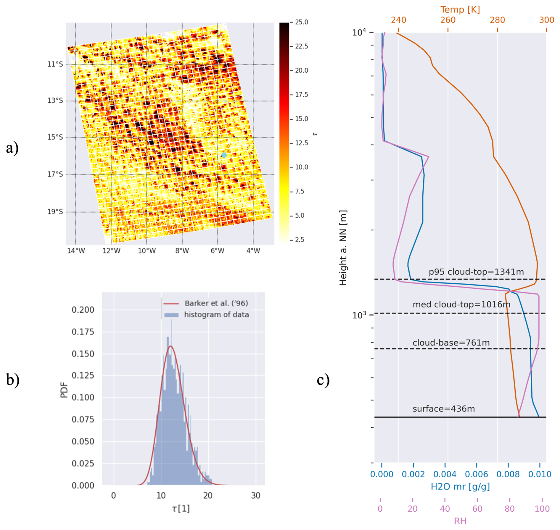
Figure 2 (a) MODIS retrieved τ above south-east Atlantic on 5 September 2014. The frame is separated into 30 × 30 km² boxes. The blue dot denotes the location of St. Helena. (b) Example of a gamma distribution of τ (red line) following Barker et al. (1996) generated using $\stackrel{\mathrm{‾}}{\mathit{\tau }}$ = 12.6 and ν = 24.1 from a 30 × 30 km² box of the MODIS frame. In blue the histogram of the τ values within the box is displayed. (c) Vertical profiles of T, relative humidity (RH) and H₂O mixing ratio from radiosonde ascent at St. Helena from 5 September 2014 at 12:00 LT. The dashed black lines indicate the cloud base and the 50th and 95th percentile of cloud tops for all 125 scenes.

For the creation of idealistic cloud scenes, gamma functions based on Barker et al. (1996) have been used to calculate PDFs of optical thickness values for the given $\stackrel{\mathrm{‾}}{\mathit{\tau }}$ and ν pair of the scene (see Fig. 2b). In total, 25 PDFs have been created based on five $\stackrel{\mathrm{‾}}{\mathit{\tau }}$ values (2.8, 4.5, 7.4, 12.2, 20.1) and five ν values between 2 and 26. In the next step, the idealistic range of τ values (p < 0.001) for the given $\stackrel{\mathrm{‾}}{\mathit{\tau }}$ and ν was extracted from each PDF, and the cloud geometrical thickness h was calculated using Eq. (13) for each τ-bin within the range.

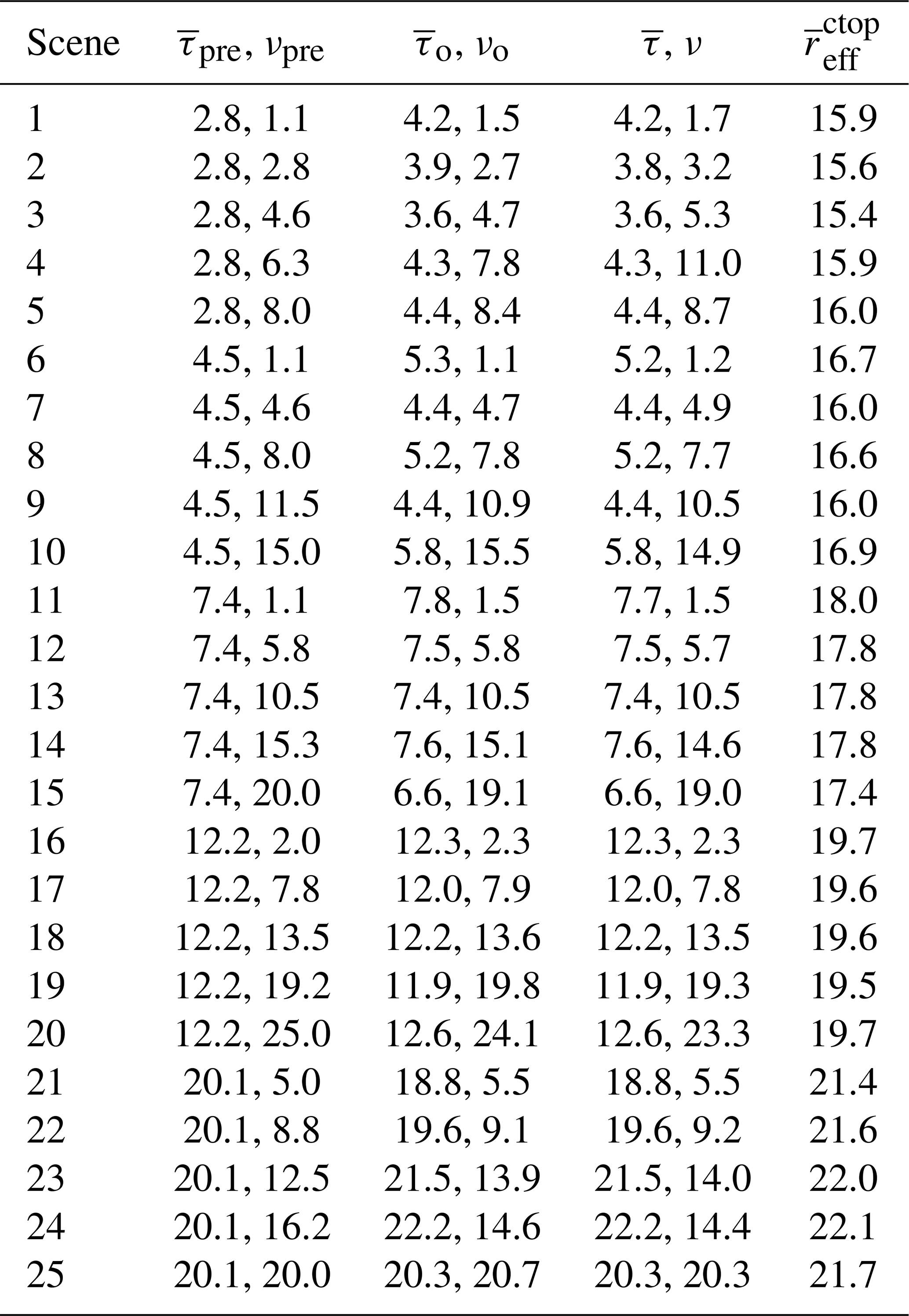
Assuming a constant cloud base and N_d, the optical thickness τ depends only on the cloud top height (Eq. 13). Using Eqs. (10) to (12) vertical profiles of LWC and r_eff are calculated for each τ-bin. The vertical resolution of the profiles is set to 25 m. For the stratocumulus deck of the MODIS frame (Fig. 2a), a very similar cloud base is assumed. Using radiosonde measurements of T, and water vapor at 12:00 LT in St. Helena, a cloud base of 761 m was assumed (see Fig. 2c). To obtain a realistic spatial distribution of cloud profiles, we found for each scene, the MODIS box with the most similar $\stackrel{\mathrm{‾}}{\mathit{\tau }}$ and ν values. The profiles are than allocated to the spatial distribution of the τ values within the box. Table A1 summarizes the pre-defined ${\stackrel{\mathrm{‾}}{\mathit{\tau }}}_{\mathrm{pre}}$ and ν_pre of the scenes, as well as the calculated values ($\stackrel{\mathrm{‾}}{\mathit{\tau }}$, ν, and ${\stackrel{\mathrm{‾}}{r}}_{\mathrm{eff}}^{\mathrm{ctop}}$) after assigning them to the MODIS boxes with the most similar values (${\stackrel{\mathrm{‾}}{\mathit{\tau }}}_{\mathrm{o}}$ and ν_o).

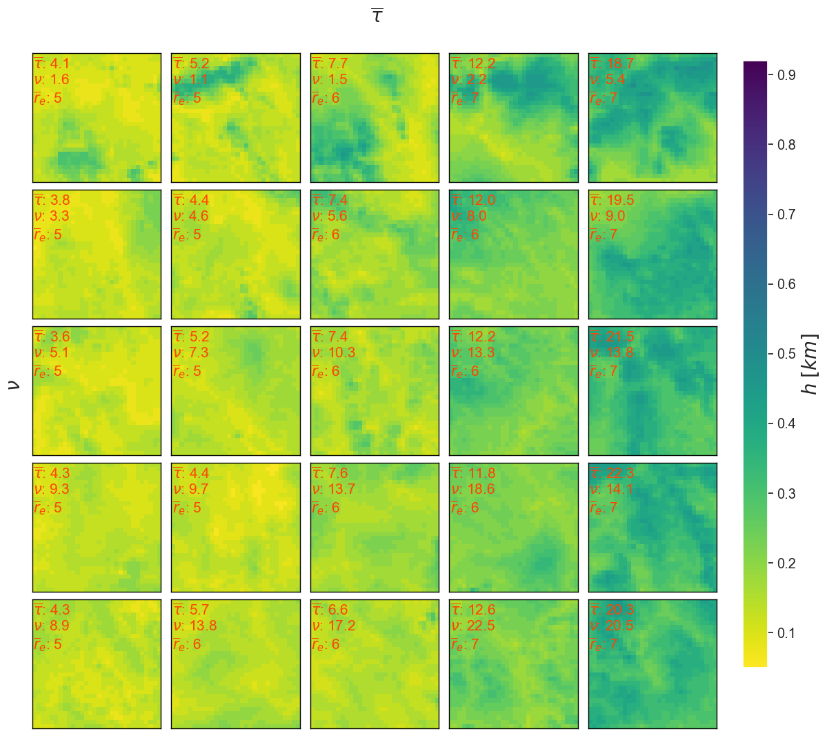
Applying five different N_d's of 25, 50, 100, 200, and 400 [cm⁻³] resulted in 125 scenes with ${\stackrel{\mathrm{‾}}{r}}_{\mathrm{eff}}^{\mathrm{ctop}}$ values ranging from 5.1 to 22.1 µm. Figures 3 and 4 display the results, showing the geometrical thickness h of the clouds for a range of $\stackrel{\mathrm{‾}}{\mathit{\tau }}$ and ν and for a N_d of 25 and 400 [cm⁻³] respectively. The values in red represent the calculated $\stackrel{\mathrm{‾}}{\mathit{\tau }}$, ν and ${\stackrel{\mathrm{‾}}{r}}_{\mathrm{eff}}^{\mathrm{ctop}}$ after assigning (see also Table A1). Comparing Fig. 3 and Fig. 4, we see that to reach the same τ, the cloud extend must be larger for larger cloud droplets (smaller N_d).

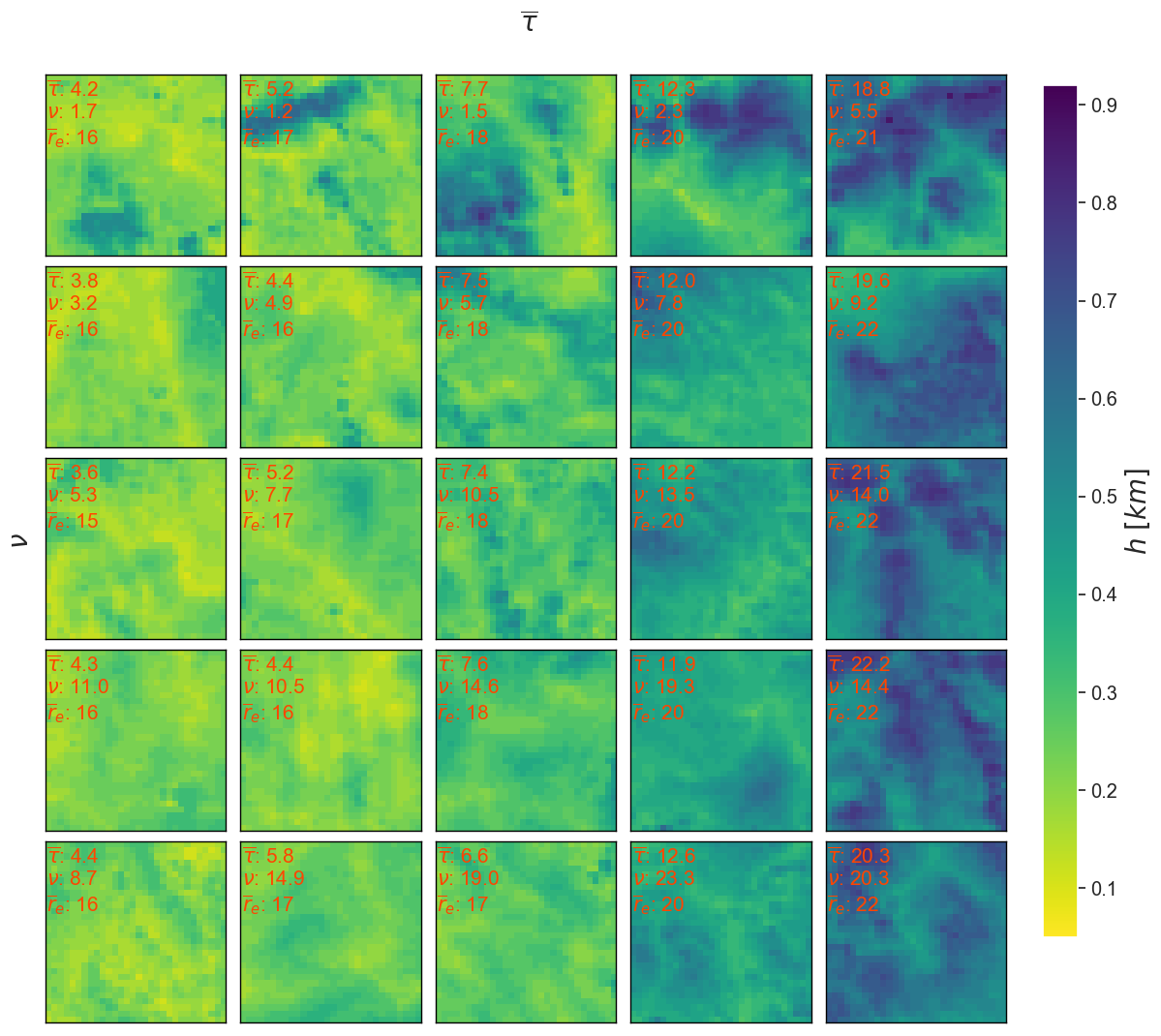
Figure 3 Cloud geometrical thickness for the 25 scenes with varying $\stackrel{\mathrm{‾}}{\mathit{\tau }}$ and ν and with the N_d set to 25 [cm⁻³]. The numbers in red represent the scene-averaged values, calculated after assigning the generated profiles to the MODIS boxes.

Figure 4 Same as Fig. 3 but with N_d of 400 [cm⁻³].

2.5 Monte Carlos Simulations

The 125 semi-synthetic scenes of cloud fields are used as inputs for a Monte Carlo Model (Marchuk et al., 1980; Barker et al., 2003) to simulate the SW TOA radiances and calculate TOA SW fluxes. For the simulations, cyclical boundary conditions are assumed. For each scene, simulations for 40 viewing zenith angles between −77 to 77° along the principal plane and for solar zenith angles of 1, 27, 55, and 75° have been performed. In total, this resulted in 20 000 scenarios. For each simulation, 10⁷ photons have been used. The ocean surface is Lambertian with a wavelength independent albedo of 0.05. For the hydrometeors, Mie-phase functions with 1800 angular-bins are used. The spectrally-dependent optical properties are computed with the model used in EarthCARE’s ACM-RT product (Cole et al., 2023).

In order to investigate the contribution of single scattering to the outgoing TOA radiance (research question 3), a histogram of the weighted fraction of the number of scattering events has been stored from the simulation for each scenario.

3 Results

In addition to flux estimates based on ADMs using the semi-physical approach (Sect. 2.2), fluxes based on the currently operational ADMs (Sect. 2.1), reconstructed in Tornow et al. (2021) and based on Su et al. (2015), are estimated. In contrast to the semi-physical ADMs, the currently operational ADMs do not explicitly take into account the cloud droplet effective radius.

The estimated fluxes are compared against Monte Carlo simulations. Figure 5 illustrates Monte Carlo simulated radiances for all scenes with N_d = 400 [cm⁻³] and for θ_v = −29° and θ_s = 27°.

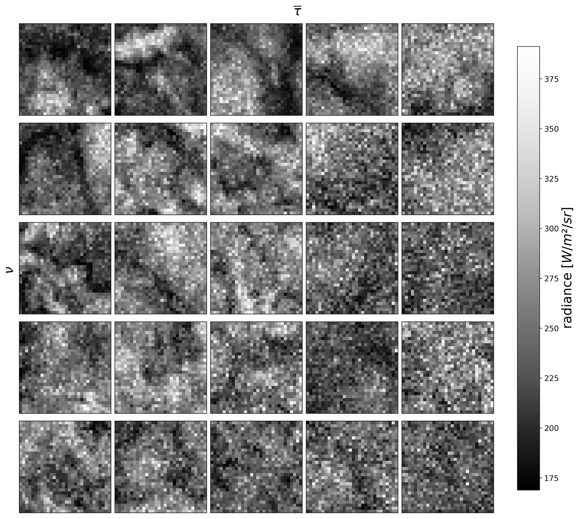
Figure 5 Monte Carlo simulations of TOA radiances for scenes in Fig. 4 and for θ_v = −29° and θ_s = 27°.

Figure 6 displays the Monte Carlo simulated and scenario-averaged radiances $I_{\mathrm{o}}({\mathit{\theta }}_{\mathrm{s}},{\mathit{\theta }}_{\mathrm{v}},\mathit{\varphi })$ (left panel) and corresponding anisotropies (right panel) at θ_s = 1° along the principal plane and for all scenes with ${\stackrel{\mathrm{‾}}{\mathit{\tau }}}_{\mathrm{pre}}$ = 2.8 and ν_pre = 8 (see Table A1) and for different N_d. We see the strong dependency of the reflected radiation from the mean cloud droplet size. We also observe single scattering features becoming apparent, such as the broadening of the cloud glory and the shift of the cloud bow towards the direct backscatter with decreasing droplet size (increasing N_d).

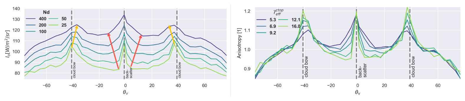
Figure 6 Left panel: mean radiance of the MCS used as I_o along θ_v (principal plane) and for varying N_d. For a θ_s = 1° and for the scene with ${\stackrel{\mathrm{‾}}{\mathit{\tau }}}_{\mathrm{pre}}$ = 2.8 and ν_pre = 8. The vertical lines indicate the location of single scattering phenomena as the cloud bow and cloud glory (around the direct backscatter). Yellow arrows indicate the shift of the cloud bow towards the direct backscatter and red arrows the broadening of the cloud glory with smaller droplets (higher N_d). Right panel: corresponding anisotropy values for the different N_d but here expressed via the mean cloud top effective radius ${\stackrel{\mathrm{‾}}{r}}_{\mathrm{eff}}^{\mathrm{ctop}}$ of the scene.

ADMs based on the sigmoidal and semi-physical approaches are constructed using the scene-averaged cloud parameters $\stackrel{\mathrm{‾}}{\mathit{\tau }}$ for the former, and additionally ${\stackrel{\mathrm{‾}}{r}}_{\mathrm{eff}}^{\mathrm{ctop}}$ for latter (see Sect. 2.1 and 2.2). All scenes are overcast (f = 1) and have ACWV = 0. With the resulting anisotropies R, SW fluxes are estimated using the spatially averaged Monte Carlo simulated radiances $I_{\mathrm{o}}({\mathit{\theta }}_{\mathrm{s}},{\mathit{\theta }}_{\mathrm{v}},\mathit{\varphi })$ (see Fig. 5).

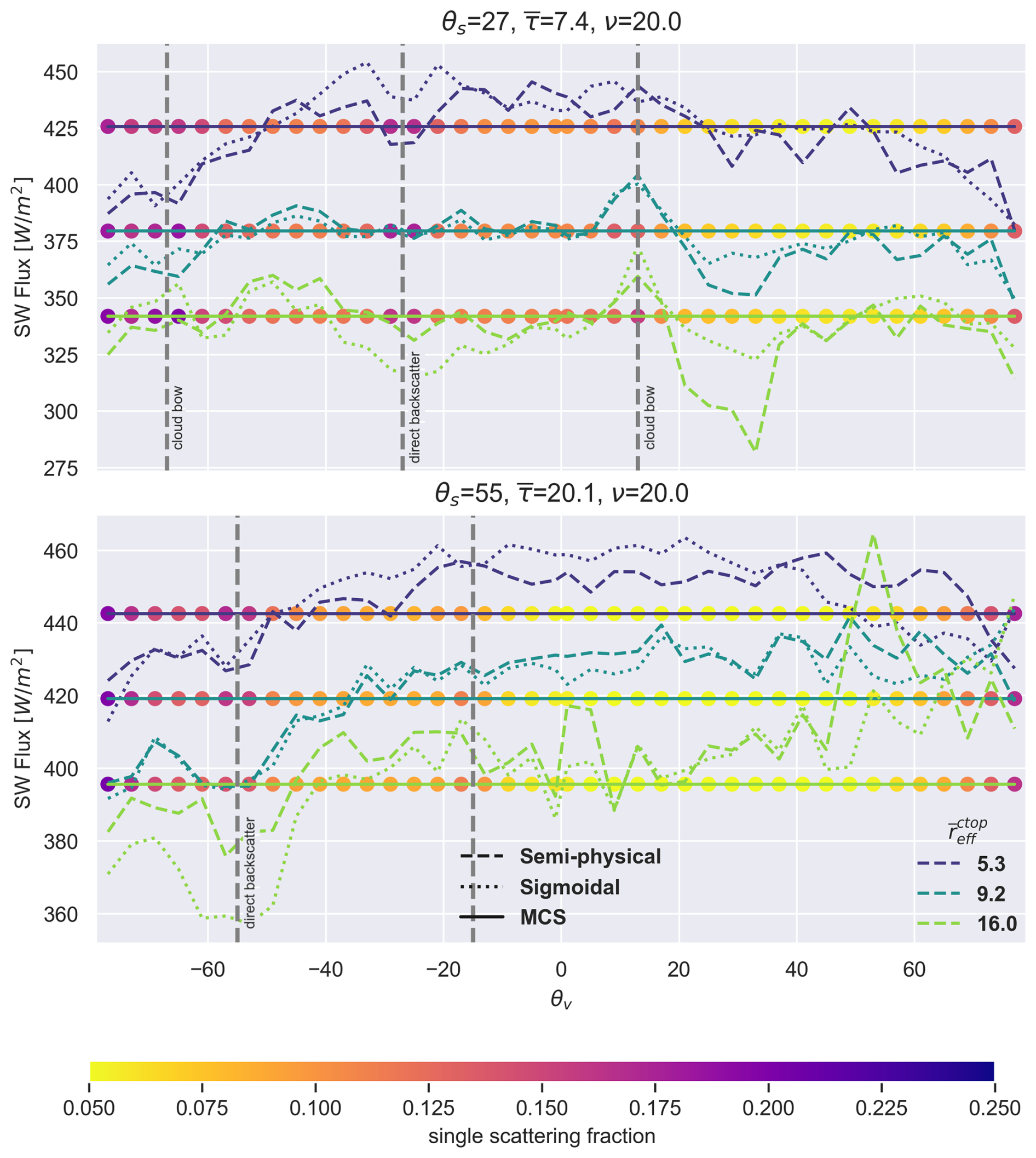
The upper panel of Fig. 7 shows the TOA SW fluxes across the principal plane for scenarios with a solar zenith angle of 1° and scenes with an optical thickness of $\stackrel{\mathrm{‾}}{\mathit{\tau }}$ = 7.4 and homogeneity of ν = 20. The solid lines show the “true” fluxes from the Monte Carlo simulations. The dashed lines represent the flux estimates based on the semi-physical approach (F_sp), and the dotted lines flux estimates based on the sigmoidal approach (F_sig). The colors of the lines illustrate estimates for scenes with different cloud effective radii. In addition, the colored dots indicate the weighted fraction of photons of the scenario that experienced single scattering before reaching TOA. The lower panel illustrates the parameterized asymmetry parameter g^Δ used for the semi-physical ADMs. The vertical lines show the location of the cloud bow and the direct backscatter, around which the cloud glory forms.

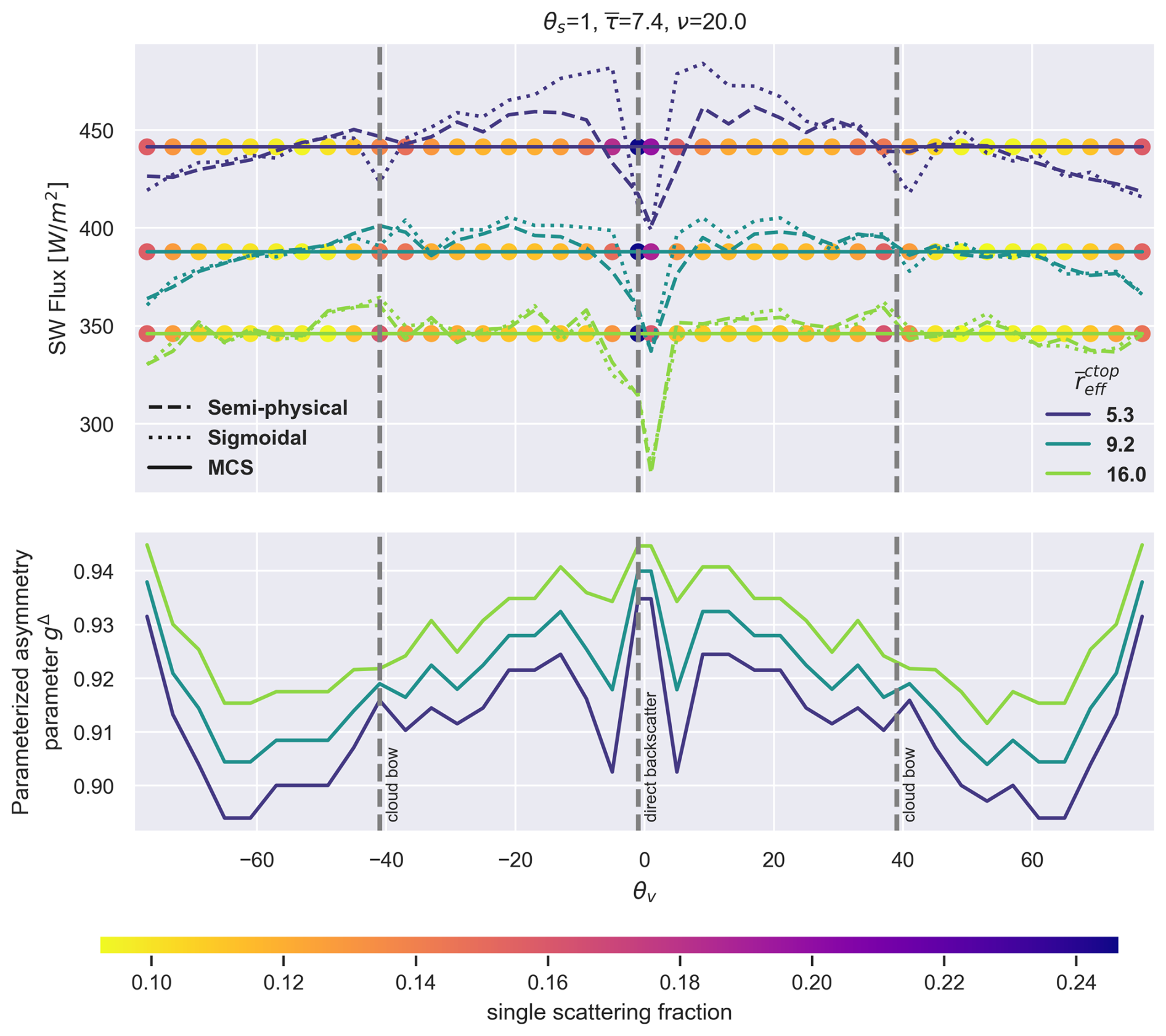
Figure 7 Upper panel: flux estimates using ADM based on the semi-physical (dashed) and based on the sigmoidal (dotted) approach for different droplet number concentrations along the principal plain. The true flux of the Monte Carlo Simulations (MCS) is shown in the solid line. The colored dots represent for each scenario the fraction of photons that has been scattered only once. Lower panel: parameterized asymmetry parameter g^Δ used for semi-physical approach.

The results show that a decrease of ${\stackrel{\mathrm{‾}}{r}}_{\mathrm{eff}}$ from 16 to 5.3 µm produces up to 100 W m⁻² higher fluxes at TOA for the same $\stackrel{\mathrm{‾}}{\mathit{\tau }}$.

Around the direct backscatter direction, where the cloud glory contributes to the observed radiance, the ADMs generated using the semi-physical approach result in flux estimates that are closer to the simulations. This is also the case at the cloud bow around ±40°. Particularly for small droplet sizes (high droplet number concentrations), where the enhanced reflectance due to single scattering effects is largest, the currently operational approach underestimates the fluxes. Due to the bin-wise optimized asymmetry parameter (bottom panel), the semi-physical approach is able to capture single scattering features such as broadening and shift in the forward direction of the cloud glory, as well as the shift towards the direct backscatter of the cloud bow with decreasing ${\stackrel{\mathrm{‾}}{r}}_{\mathrm{eff}}$ (Tornow et al., 2021). The results illustrate that this leads to more accurate flux estimates in these geometries comparing to the sigmoidal approach.

For angles influenced by the cloud bow or cloud glory, an enhanced contribution of single scattering (colored dots) to the reflected radiance is clearly visible. Furthermore, the single scattering fraction increases with decreasing ${\stackrel{\mathrm{‾}}{r}}_{\mathrm{eff}}$. This underpins the hypothesis that the adjustments of g^Δ (lower panel) during the bin-wise optimization procedure (Tornow et al., 2020) are primarily attributable to perceived single scattering effects, such as the broadening and shift of the cloud glory and the shift of cloud bow.

Figure 8 shows the results for θ_s for 27 and 55° with similar results. At geometries influenced by the cloud glory, the sigmoidal approach performs well under average microphysical conditions (e.g, ${\stackrel{\mathrm{‾}}{r}}_{\mathrm{eff}}$ ≈ 10 µm) but overestimates the fluxes at high and underestimates them at low ${\stackrel{\mathrm{‾}}{r}}_{\mathrm{eff}}$. This agrees with Fig. 1 where the predicted radiances using the sigmoidal approach (right panel) correspond well with the semi-physical approach using a typical mean effective radius of 10 µm (second panel) but are lower for small droplets (first panel) and higher for large droplets (third panel).

Figure 8 As Fig. 7 upper panel but for a θ_s of 27 and 55°.

At high and low θ_v, both approaches struggle because fewer training data was available for these geometries. In sun-glint affected geometries both approaches have problems in estimate accurately the fluxes, but the semi-physical approach generally deviates even more. These findings are consistent with higher uncertainties of the models for these geometries found in Tornow et al. (2020).

In Fig. 9, the flux deviations for scenes with a N_d of 400 cm⁻³ and the corresponding highest homogeneity are illustrated for varying $\stackrel{\mathrm{‾}}{\mathit{\tau }}$ and θ_s. The upper panel displays the deviation of the flux estimates using semi-physical (ΔF_sp) and the lower panel using sigmoidal based ADMs (ΔF_sig). In the top of each panel, the average over all $\stackrel{\mathrm{‾}}{\mathit{\tau }}$ (black line) and the standard deviation (gray shadows) are shown. The doted isoline indicates areas where the differences exceed the EarthCARE mission goal of ±10 W m⁻².

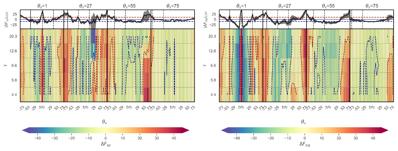
Figure 9 Deviation of fluxes estimated (ΔF = F_MCS − F_est) using ADM's based on the semi-physical approach (upper panel) and on the sigmoidal approach (lower panel) from the fluxes of MCS along the principal plane and for varying θ_s and $\stackrel{\mathrm{‾}}{\mathit{\tau }}$. The N_d of the scenes is 400 [cm⁻³] and for ν always the scene with the highest homogeneity is selected. The dotted blue and red lines represent the −10 and 10 W m⁻² threshold. On top of each panel the deviation averaged over all optical thicknesses is shown. The shaded areas mark the 5th and 95th percentiles. The vertical lines indicate the direct backscatter and the cloud bow (θ_s ± 40°).

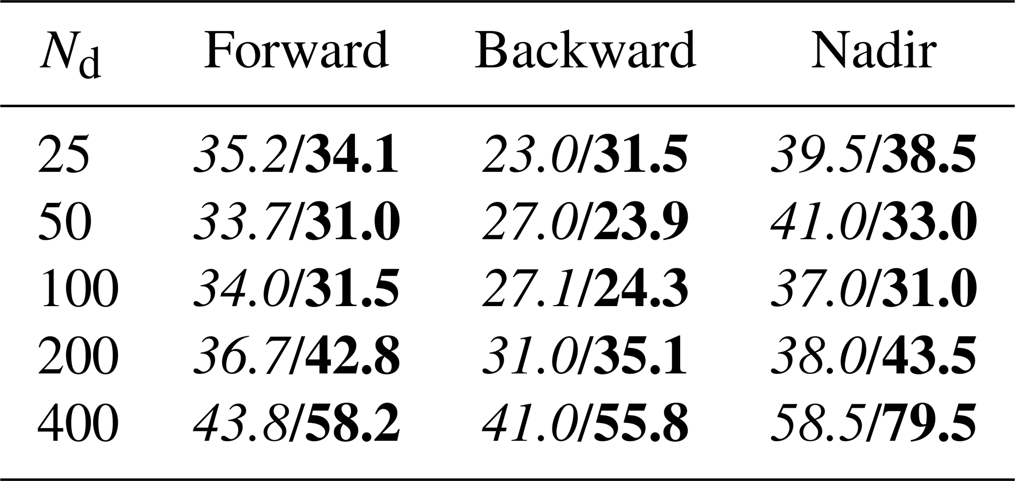
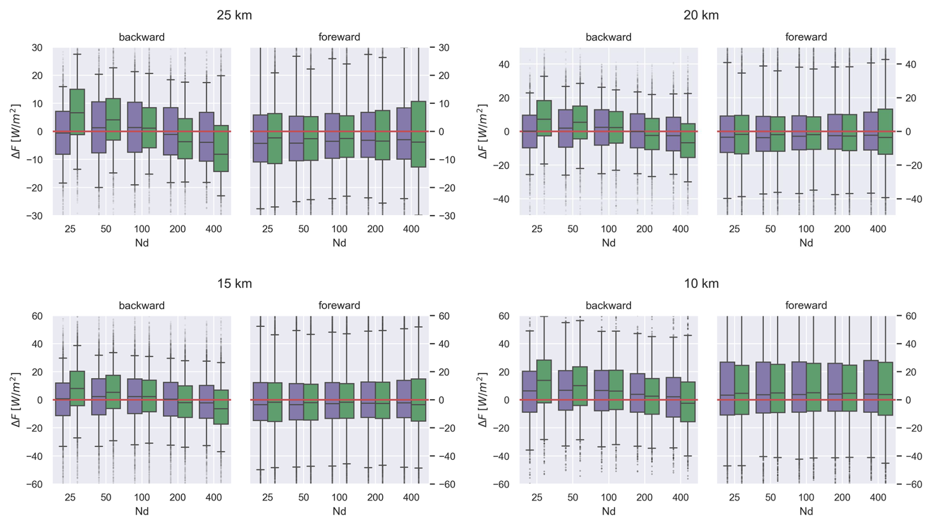
In general, the semi-physical approach deviates less from the simulations, particularly in viewing geometries around the cloud glory and cloud bow. This is the case for all optical thicknesses and solar zenith angles, but for small $\stackrel{\mathrm{‾}}{\mathit{\tau }}$ the effect is more distinctive. The deviations in instantaneous flux estimates using the semi-physical approach compared to the currently operational approach can be reduced by up to 25 W m⁻² or even more. In the sun glint affected geometries, both approaches show large uncertainties. Both absolute and relative deviations (not shown) increase with smaller $\stackrel{\mathrm{‾}}{\mathit{\tau }}$ in this region. This indicates that even in overcast cases, with high optical thicknesses, the sun-glint significantly influences the TOA radiances. Figure 10 illustrates for each θ_s the box-whisker plots (n = 500) of flux deviations (ΔF) for scenarios in the backward (left) and forward direction (right), and for different droplet number concentrations. Particularly at extreme N_d (e.g., 25 and 400 cm⁻³), the semi-physical approach deviates less from the simulations in the backward direction. For this cases the median deviation of the 5000 scenarios can be reduced by up to 7 W m⁻² (such as for θ_s = 55° and N_d). This can be explained by the fact that the sigmoidal approach does not explicitly take N_d into account. By using observations independently on their microphysics, the sigmoidal approach produces in the backward direction best estimates at average N_d such as 50 and 100 cm⁻³, but is less accurate in extreme high or low N_ds. For the forward direction where single scattering features are less important, the sigmoidal approach generally does not perform better. Table 2 lists the probability of ΔF > 10 W m⁻² for scenes with different N_d and for scenarios calculated for the backward, forward and nadir direction. For high N_d the semi-physical approach can reduce the probability by up to 20 %. The mean absolute relative error was found to decrease with increasing $\stackrel{\mathrm{‾}}{\mathit{\tau }}$ and ν, and to increase with larger θ_s and, particularly for the sigmoidal approach, with decreasing ${\stackrel{\mathrm{‾}}{r}}_{\mathrm{eff}}^{\mathrm{ctop}}$ (increasing N_d) (not shown). In Fig. 11 the 30 × 30 km² scenes (θ_s = 55°) have been divided into subdomains with sizes of 25, 20, 15 and 10 km to explore the dependency of the flux estimates on domain size. The variability in ΔF increases with smaller domain sizes. As in the case of 30 km, the semi-physical approach produces better estimates in the backward direction and for domains with extremely high or low ${\stackrel{\mathrm{‾}}{r}}_{\mathrm{eff}}^{\mathrm{ctop}}$ (N_d) for all resolutions. For a domain size of 10 × 10 km² both approaches show a positive bias. As EarthCARE's assessment domain has a size of 100 km², the results might be of interest for the validation of the BMA-FLX product.

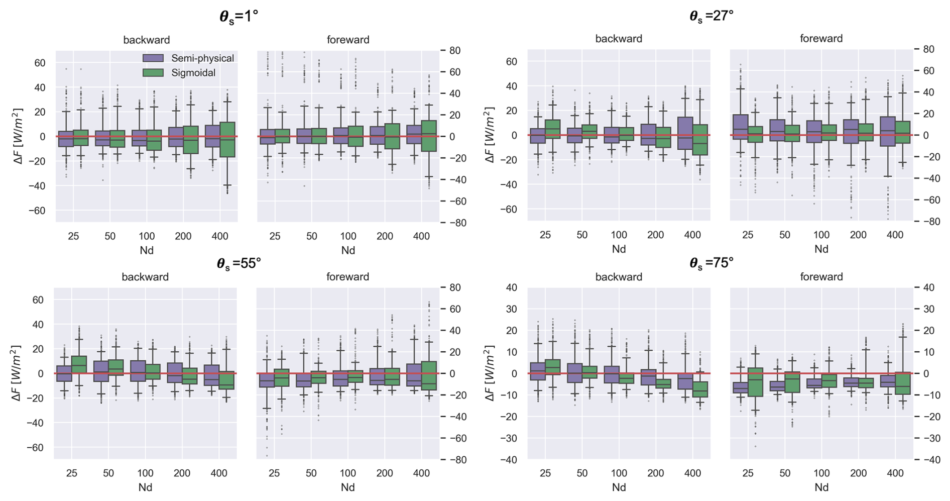
Figure 10 Box-Whisker plots showing flux deviations for the different θ_s using n = 500 scenes of all $\stackrel{\mathrm{‾}}{\mathit{\tau }}$ and ν and for the left side of each panel of −77 < θ_v < 0 and for the right side 0 < θ_v < 77. The upper and lower limits represent the 95th and 5th percentiles.

Table 2 Table showing the probability in % of ΔF > 10 W m⁻². Forward includes all scenarios of 0 < θ_v < 77, backward of 0 > θ_v > −77 and nadir of −1 < θ_v < 1. The italic numbers are for the semi-physical approach and bold numbers for the sigmoidal approach.

Figure 11 As Fig. 10 with θ_s = 55° but for domain sizes of 25, 20, 15 and 10 km.

4 Conclusion and Discussion

In this study, Top of Atmosphere (TOA) shortwave (SW) radiances are simulated along the principal plane for 125 semi-synthetic 3D scenes of marine boundary layer stratocumulus clouds with varying mean cloud optical thickness, cloud homogeneities, and mean effective radius. Seeking TOA SW flux closure above liquid clouds, two sets of ADMs based on the semi-physical (Tornow et al., 2021, 2020) and sigmoidal approach (Su et al., 2015) are compared against the fluxes calculated using a Monte Carlo Model (Marchuk et al., 1980; Barker et al., 2003).

Averaged over all analyzed scenarios, the mean absolute relative error decreases with increasing $\stackrel{\mathrm{‾}}{\mathit{\tau }}$ and ν, and increases with increasing θ_s and, particularly for the sigmoidal approach, with decreasing ${\stackrel{\mathrm{‾}}{r}}_{\mathrm{eff}}^{\mathrm{ctop}}$ (Research question 1). Furthermore, the microphysically aware semi-physical approach reduces the errors in instantaneous flux estimates by up to 25 W m⁻² compared to the sigmoidal approach. The improvements are found to be largest for geometries in the backward direction and for scenes where microphysics deviated most from mean conditions, such as scenes with extremely high or low ${\stackrel{\mathrm{‾}}{r}}_{\mathrm{eff}}^{\mathrm{ctop}}$ (N_d). The median deviation of these scenarios (backward direction and different N_d, n = 500) is improved for all θ_s and N_d by up to 7 W m⁻². Although this study only covers the principal plane, the results show the potential of improving SW flux estimates by explicitly incorporating cloud microphysics in ADMs. Similar results have been found in Tornow et al. (2021), where the two radiance-to-irradiance approaches have been compared using satellite data (Research question 2). Analyzing the Monte Carlo Simulations (MCS), the adjustments of the parameterized asymmetry parameter g^Δ could be related to changes in the fraction of single scattering events contributing to the TOA radiance signal. The changes in the single scattering fraction are associated with phenomena such as cloud bow or cloud glory, which depend on cloud microphysical properties (Research question 3).

By explicitly incorporating cloud microphysical properties through the effective radius, the semi-physical approach substantially reduces flux estimation errors for the investigated scenarios, particularly for those affected by single-scattering phenomena such as the cloud glory and the cloud bow. As these phenomena are strongest in the backward direction, the improvements compared to the currently operational approach are most pronounced in scenarios with corresponding observational geometries. For sun glint affected geometries, the flux estimates show large variabilities, and any interpretation should be done with caution.

Using the optimized g^Δ, the semi-physical approach is able to capture the shift of the cloud bow and the broadening of the cloud glory with decreasing droplet size, explaining the more accurate estimates in these geometries.

The findings of this study encourage further research on microphysically aware ADMs. For the radiative closure experiment of the EarthCARE mission, launched in May 2024 (Wehr et al., 2023), the semi-physical approach shows potential to improve SW flux estimates. EarthCARE aims to achieve radiative closure by comparing simulated fluxes from active and passive instruments aboard the satellite with estimates from the broadband radiometer (BBR) (Velázquez Blázquez et al., 2024b). Particularly for observational geometries in the backward-scattering direction, the semi-physical approach reduces potential misinterpretations of flux deviations that exceed the mission goal of 10 W m⁻², but actually arise from uncertainties in the SW flux estimates. Although EarthCARE’s observational geometries lie outside the principal plane investigated in this study (e.g., Tornow et al., 2019), they are likewise influenced by variations in cloud microphysics and single-scattering phenomena.

When assessing radiative closure with EarthCARE, it is important to remember that BBR-based fluxes are estimates rather than direct measurements, and that their uncertainties depend on surface type, atmospheric conditions, and sun–satellite geometry. For low ${\stackrel{\mathrm{‾}}{r}}_{\mathrm{eff}}^{\mathrm{ctop}}$ (high N_d), the semi-physical approach substantially reduces the probability of ΔF > 10 W m⁻². For both approaches, flux uncertainties increase with decreasing footprint size. Future work should further investigate the sensitivities to footprint size, retrieval errors (e.g., of above-cloud water vapor and r_eff), noise, and varying observational conditions.

Overall, the results highlight that explicitly incorporating cloud microphysical information into ADMs is a promising pathway for improving TOA SW flux estimates above clouds. Unlike previous Earth radiation budget missions that focused mainly on minimizing global flux biases, EarthCARE’s emphasis on radiative closure may particularly benefit from microphysically aware instantaneous flux estimates.

Appendix A

Table A1 Table showing pre-selected ${\stackrel{\mathrm{‾}}{\mathit{\tau }}}_{\mathrm{pre}}$, ν_pre for the 25 scenes and the calculated $\stackrel{\mathrm{‾}}{\mathit{\tau }}$, ν and ${\stackrel{\mathrm{‾}}{r}}_{\mathrm{eff}}^{\mathrm{ctop}}$ after assigning the profiles to the boxes of MODIS observations with the most similar ${\stackrel{\mathrm{‾}}{\mathit{\tau }}}_{\mathrm{o}}$, ν_o values. The calculated values are for the scenes with N_d = 25.