A weighted least squares approach to retrieve aerosol layer height over bright surfaces applied to GOME-2 measurements of the oxygen A band for forest fire cases over Europe

This paper presents a weighted least squares approach to retrieve aerosol layer height from top-of-atmosphere reflectance measurements in the oxygen A band (758–770 nm) over bright surfaces. A property of the measurement error covariance matrix is discussed, due to which photons travelling from the surface are given a higher preference over photons that scatter back from the aerosol layer. This is a potential source of biases in the estimation of aerosol properties over land, which can be mitigated by revisiting the design of the measurement error covariance matrix. The alternative proposed in this paper, which we call the dynamic scaling method, introduces a scene-dependent and wavelength-dependent modification in the measurement signal-to-noise ratio in order to influence this matrix. This method is generally applicable to other retrieval algorithms using weighted least squares. To test this method, synthetic experiments are done in addition to application to GOME-2A and GOME-2B measurements of the oxygen A band over the August 2010 Russian wildfires and the October 2017 Portugal wildfire plume over western Europe.

1 Introduction

Algorithms that estimate properties of atmospheric species from satellite measurements of top-of-atmosphere (TOA) radiance (including spectral signatures of gases) in planetary atmospheres typically employ an inverse method based on least squares. When retrieving terrestrial properties, this approach requires spectrally resolved measurements of the TOA Earth radiance, solar irradiance and a forward model as the minimal base ingredients with which the state vector parameters can be retrieved (which are also model parameters). The goal of the least squares approach is to minimize a cost function, which aims to reduce discrepancies between the forward model and the measurement by iteratively manipulating state vector parameters. Upon minimization, the iterative scheme converges to a solution that, in principle, best describes the forward model's representation of the measurement.

Many atmospheric retrieval algorithms employ a weighted least squares estimation (WLSE) method modified to include a priori information on the state vector. An example of such an inverse method set-up is optimal estimation (Rodgers, 2000), which is an attractive method particularly because of its efficacy in providing a posteriori error statistics on the retrieved parameter. The KNMI aerosol layer height (ALH) retrieval algorithm uses an inverse method based on OE and exploits the spectral structure of the near-infrared spectrum of the top-of-atmosphere radiance between 758 and 770 nm, where photons travelling through the Earth's atmosphere predominantly get absorbed by molecular oxygen. Oxygen is a well-mixed gas and the spectral structure of its absorption lines is pressure-dependent (Min and Harrison, 2004). The further the light in the oxygen A band passes through the atmosphere, the more it gets absorbed until it interacts with scattering species (such as clouds and aerosols) and scatters back to the TOA. It is this feature of the oxygen A band that has made it an attractive wavelength region for retrieving aerosol information (Corradini and Cervino, 2006; Frankenberg et al., 2012; Gabella et al., 1999; Hollstein and Fischer, 2014; Pelletier et al., 2008; Sanders and de Haan, 2013, 2016; Sanders et al., 2015; Sanghavi et al., 2012; Wang et al., 2012). The algorithm is operational for the TROPOspheric Monitoring Instrument (TROPOMI) on board the Sentinel-5 Precursor (S5P) mission (Veefkind et al., 2012) and is also a part of the Sentinel-4 (S4) and Sentinel-5 (S5) missions (Ingmann et al., 2012) under the Copernicus satellite programme of the European Union.

Due to the large spectral variability in absorption within the oxygen A band, the measured TOA radiance and the measurement noise have a high dynamic range. The minimization of the propagation of measurement noise to the final retrieval solution should be a critical component of any retrieval algorithm. In WLSE, this is accomplished by the inverse measurement error covariance matrix, which ranks the measurement on each detector pixel using the information available on the measurement noise. Due to the extent of the dynamic range of the measurement noise in the oxygen A band, this ranking matrix becomes a primary controlling entity; if the measurement noise is very large, the inverse noise variance is very low, which results in a lower rank to the measured signal from that specific detector pixel.

Since the measured signal is scene dependent, the spectral rank of each detector pixel is also scene dependent. This has special consequences over bright surfaces, where the dynamic range of the measured signal is much larger than over dark surfaces. Due to this, photons at wavelengths where the oxygen A band has a lower absorption cross section are less absorbed (subsequently travelling further into the atmosphere) and have a much larger representation in the WLSE method. A consequence of this, reported by Nanda et al. (2018), is that the retrieved ALH values are inaccurate for measurements over land.

In order to account for unknown instrument and model errors, Sanders et al. (2015) multiply the measurement error from L1b by two for their GOME-2 case studies and by 10 in SCIAMACHY case studies for retrieving ALH over ocean and land. They observe that increasing the measurement noise results in an increase in the number of retrieval convergences without significantly decreasing the accuracy of the retrieved ALH for the already converged solutions. The method utilized by Sanders et al. (2015) does not change the shape of the noise spectrum since it is multiplied by a constant. This paper investigates a vector-based weighing scheme (we call it the dynamic scaling method, as opposed to the formal approach which is unscaled OE), which dynamically varies from scene to scene and changes the shape of the noise spectrum itself. The objective of the dynamic scaling method is to influence the inverse measurement error covariance matrix in its ranking of the instrument's detector pixels in its spectral dimension in order to maximize sensitivity to the ALH. The study discussed in this paper is a part of a series of papers discussing the ALH retrieval algorithm developed at the KNMI (Nanda et al., 2018; Sanders and de Haan, 2013, 2016; Sanders et al., 2015).

The retrieval algorithm is described in Sect 2, which provides a description of the forward model and the formalism of OE. The incompatibility of retrieving aerosol properties from oxygen A band measurements with the formal design of the measurement error covariance matrix are briefly discussed in the same section (Sect. 2) before a full description of the proposed method in Sect 3 and a demonstration in a synthetic environment in Sect 4 are given. This method is applied to real data in Sect 5. The Russian wildfires in August 2010, which were discussed by Nanda et al. (2018), are revisited to compare the two approaches. The data are derived from the GOME-2A (Global Ozone Monitoring Experiment on board the MetOp-A platform of the European Organisation for the Exploitation of Meteorological Satellites, EUMETSAT) instrument and validated with a co-located CALIPSO (Cloud-Aerosol Lidar and Infrared Pathfinder Satellite Observation of the National Aeronautics and Space Administration, NASA) overpass. The dynamic scaling method is further applied to the Portugal fire plumes over western Europe on 17 October 2017 using data from the GOME-2B instrument, with validation from the ground-based European Meteorological Services Network (Alexander et al., 2016) ceilometer network in the Netherlands and Germany, along with radiosonde measurements of the relative humidity profile and the back trajectory of the aerosol plumes. This demonstration is followed by the conclusion in Sect. 6.

2 The ALH retrieval algorithm

The algorithm is comprised of a forward model and an inverse method. The forward model uses a radiative transfer model described by de Haan et al. (1987) to calculate the top-of-atmosphere (TOA) Earth radiance (I) in the oxygen A band. This is done by propagating incoming solar irradiance (E₀) in the oxygen A band through the Earth's atmosphere, which is described by an atmospheric model. Finally, this model is fitted to the measured spectrum to retrieve the primary unknown ALH while fitting the aerosol optical thickness (AOT). For more details, the reader may refer to Sanders et al. (2015).

2.1 The forward model

The atmospheric model describes the interaction of photons with various components of the Earth's atmosphere that either absorb photons or scatter them in different directions. The oxygen absorption cross sections are derived from the NASA Jet Propulsion Laboratory database, and first-order line mixing and collision-induced absorption between O₂-O₂ and O₂-N₂ are defined from Tran et al. (2006) and Tran and Hartmann (2008). The scattering species in the atmosphere include gases and molecules that follow Rayleigh-scattering principles, aerosols, clouds and the surface. At present, the algorithm assumes cloud-free scenes, since the presence of clouds can result in large biases in the retrieved ALH (Sanders and de Haan, 2016; Sanders et al., 2015). Aerosols are modelled as a single layer with a fixed thickness of 50 hPa. ALH is defined as the medium pressure of the aerosol layer, converted to a height above the ground. The aerosol layer has a constant aerosol extinction coefficient and a fixed aerosol single-scattering albedo (ω). Scattering by aerosols is described by a Henyey–Greenstein phase function (Henyey and Greenstein, 1941) with an anisotropy factor g of 0.7. This choice is motivated by the model's simplicity in describing scattering, which facilitates faster radiative transfer calculations than a more complex Mie-scattering model. Currently, the surface is modelled as Lambertian.

The radiative transfer calculations are done line by line within the wavelength range of 758–770 nm, which requires a large computational effort for a single retrieval per iteration. In order to reduce computational time per iteration, polarization is ignored. This is a viable step, since the Rayleigh-scattering cross section is very low in the near-infrared region. Because of the low Rayleigh-scattering cross section in the near-infrared, Rotational Raman-scattering can also be ignored.

The solar irradiance and Earth radiance are convolved with an instrument spectral response function (ISRF) f_ISRF(λ−λ_i) to simulate a spectrum observed by a satellite instrument. The TOA reflectance (R) is computed as

$$\begin{array}{}\text{(1)}& {\displaystyle }{\displaystyle }{y}_i=R\left({\mathit{\lambda }}_i\right)={\displaystyle \frac{\mathit{\pi }}{{\mathit{\mu }}_{\mathrm{0}}}}{\displaystyle \frac{\int f_{\text{ISRF}}(\mathit{\lambda }-{\mathit{\lambda }}_i)I\left(\mathit{\lambda }\right)\mathrm{d}\mathit{\lambda }}{\int f_{\text{ISRF}}(\mathit{\lambda }-{\mathit{\lambda }}_i)E_{\mathrm{0}}\left(\mathit{\lambda }\right)\mathrm{d}\mathit{\lambda }}},\end{array}$$

where μ₀ is the cosine of the solar zenith angle θ₀, and the subscript i is the index of the spectral channel. For a more in-depth description of the forward model, please refer to Sanders et al. (2015). All synthetic spectra presented in this paper are from a hypothetical instrument with a Gaussian ISRF and a spectral resolution (FWHM) of 0.11 nm oversampled by a factor of 3. These specifications are very similar to the Sentinel-4 Ultraviolet Visible and Near infrared (UVN) instrument. The sensitivity analyses conducted in this paper may also be applicable to instruments with a lower spectral resolution. Further on in this paper, experiments are conducted with measured spectra from the GOME-2A and B instruments, which have a lower spectral resolution than the S4 UVN instrument.

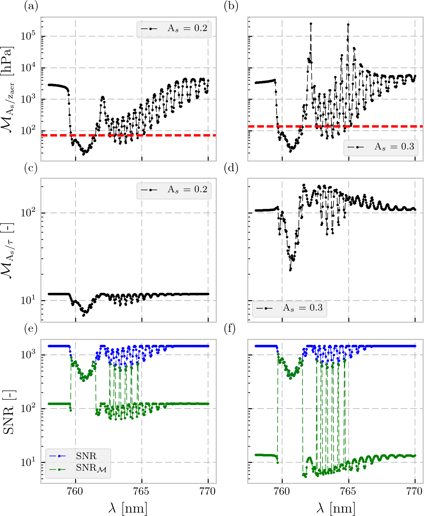
Figure 1 (a, b) Modifying vector ${\mathcal{M}}_{A_{\mathrm{s}}/z_{\text{aer}}}$ as a function of wavelength λ. The solar zenith angle is 45^∘, the viewing zenith angle is 20^∘ and the relative azimuth angle is 0^∘. The aerosol optical thickness (τ) is 0.5 at 760 nm over a surface with an albedo of 0.2 (a, c, e) and 0.3 (b, d, f) at 760 nm. The height of the aerosol layer is 900 hPa with a pressure thickness of 200 hPa. The aerosol single-scattering albedo is 0.95 and the aerosol scattering is described by a Henyey–Greenstein phase function with an asymmetry factor of 0.7. The red dashed line represents the modification threshold value 𝒯, which has been set at the 20th percentile of ${\mathcal{M}}_{A_{\mathrm{s}}/z_{\text{aer}}}$ in this example. (c, d) Modifying function ${\mathcal{M}}_{A_{\mathrm{s}}/\mathit{\tau }}$, Eq. (8) as a function of wavelength. (e, f) The blue line represents the unscaled SNR, whereas the green line represents the modified SNR according to Eq. (7).

2.2 The formal ALH inverse method

OE is a maximum a posteriori (MAP) estimator designed to find a solution for unknowns x in the classic inverse problem described in Eq. (2) as

$$\begin{array}{}\text{(2)}& {\displaystyle }{\displaystyle }\mathit{y}=\mathbf{F}(\mathit{x},\mathit{b})+\mathit{ϵ},\end{array}$$

where y is the vector of measurements (in this case, reflectance in the oxygen A band as a function of spectral channel index), F(x,b) is the aforementioned forward model with the state vector x and other model parameters b, and ϵ represents the measurement noise (at each spectral point). The OE method, being a MAP estimator, requires the knowledge of a priori errors in the estimation parameters. These errors are represented by the a priori error covariance matrix S_a and the measurement noise covariance matrix S_ϵ. Because measurement noise is considered uncorrelated, S_ϵ is diagonal. S_a is also considered diagonal since the state vector elements are assumed to be uncorrelated. The inverse method propagates these errors into the a posteriori error covariance matrix $\widehat{\mathbf{S}}$ following Eq. (3):

$$\begin{array}{}\text{(3)}& {\displaystyle }{\displaystyle }\widehat{\mathbf{S}}={\left({\mathbf{K}}^T{\mathbf{S}}_{\mathit{ϵ}}^{-\mathrm{1}}\mathbf{K}+{\mathbf{S}}_{\mathrm{a}}^{-\mathrm{1}}\right)}^{-\mathrm{1}},\end{array}$$

with K as the Jacobian or the matrix of partial derivatives of F(x,b) with respect to the state vector parameters x at the retrieval solution. Since the forward model is non-linear, a Gauss–Newton method is employed to minimize the cost function (Eq. 4) towards a zero gradient:

$$\begin{array}{ll}{\displaystyle }& {\displaystyle }{\mathit{\chi }}^{\mathrm{2}}=[\mathit{y}-\mathbf{F}(\mathit{x},\mathit{b}\left){]}^T{\mathbf{S}}_{\mathit{ϵ}}^{-\mathrm{1}}\right[\mathit{y}-\mathbf{F}(\mathit{x},\mathit{b})]\\ \text{(4)}& {\displaystyle }& {\displaystyle }+(\mathit{x}-{\mathit{x}}_{\mathrm{a}}{)}^T{\mathbf{S}}_{\mathrm{a}}^{-\mathrm{1}}(\mathit{x}-{\mathit{x}}_{\mathrm{a}}),\end{array}$$

with x_a as the a priori state vector. The update to the state vector x_n+1 for iteration n is provided in Eq. (5):

$$\begin{array}{ll}{\displaystyle }& {\displaystyle }{\mathit{x}}_{n+\mathrm{1}}={\mathit{x}}_{\mathrm{a}}+({\mathbf{K}}_n^T{\mathbf{S}}_{\mathit{ϵ}}^{-\mathrm{1}}{\mathbf{K}}_n+{\mathbf{S}}_{\mathrm{a}}^{-\mathrm{1}}{)}^{-\mathrm{1}}{\mathbf{K}}_n^T{\mathbf{S}}_{\mathit{ϵ}}^{-\mathrm{1}}\\ \text{(5)}& {\displaystyle }& {\displaystyle }[\mathit{y}-\mathbf{F}({\mathit{x}}_n,\mathit{b})+{\mathbf{K}}_n({\mathit{x}}_n-{\mathit{x}}_{\mathrm{a}}\left)\right],\end{array}$$

where K_n is the Jacobian at the nth iteration and x_n is the state vector at the nth iteration. The retrieval is said to converge to a solution when the state vector update is lower than the expected precision. The matrix S_ϵ plays a very important role in the WLSE framework by essentially ranking each spectral point based on the absolute measurement error in order to reduce the effect of measurement noise in the retrieved parameter. This is done by the ${\mathbf{S}}_{\mathit{ϵ}}^{-\mathrm{1}}$ matrix, which assigns a relatively higher value for spectral points with a lower noise covariance and vice versa. The spectral points with a higher ${\mathbf{S}}_{\mathit{ϵ}}^{-\mathrm{1}}$ value essentially have an overall stronger influence in the WLSE. The design of this WLSE framework makes the retrieval solution intrinsically dependent on the quality of the ${\mathbf{S}}_{\mathit{ϵ}}^{-\mathrm{1}}$ matrix. This matrix will always rank higher those spectral points that represent photons less absorbed by oxygen, i.e. those which travel through the atmosphere more easily, as the relative error at these spectral points is low. Because aerosols are weak scatterers of light, a large fraction of photons pass through the aerosol layer and interact with the surface before returning to the detector.

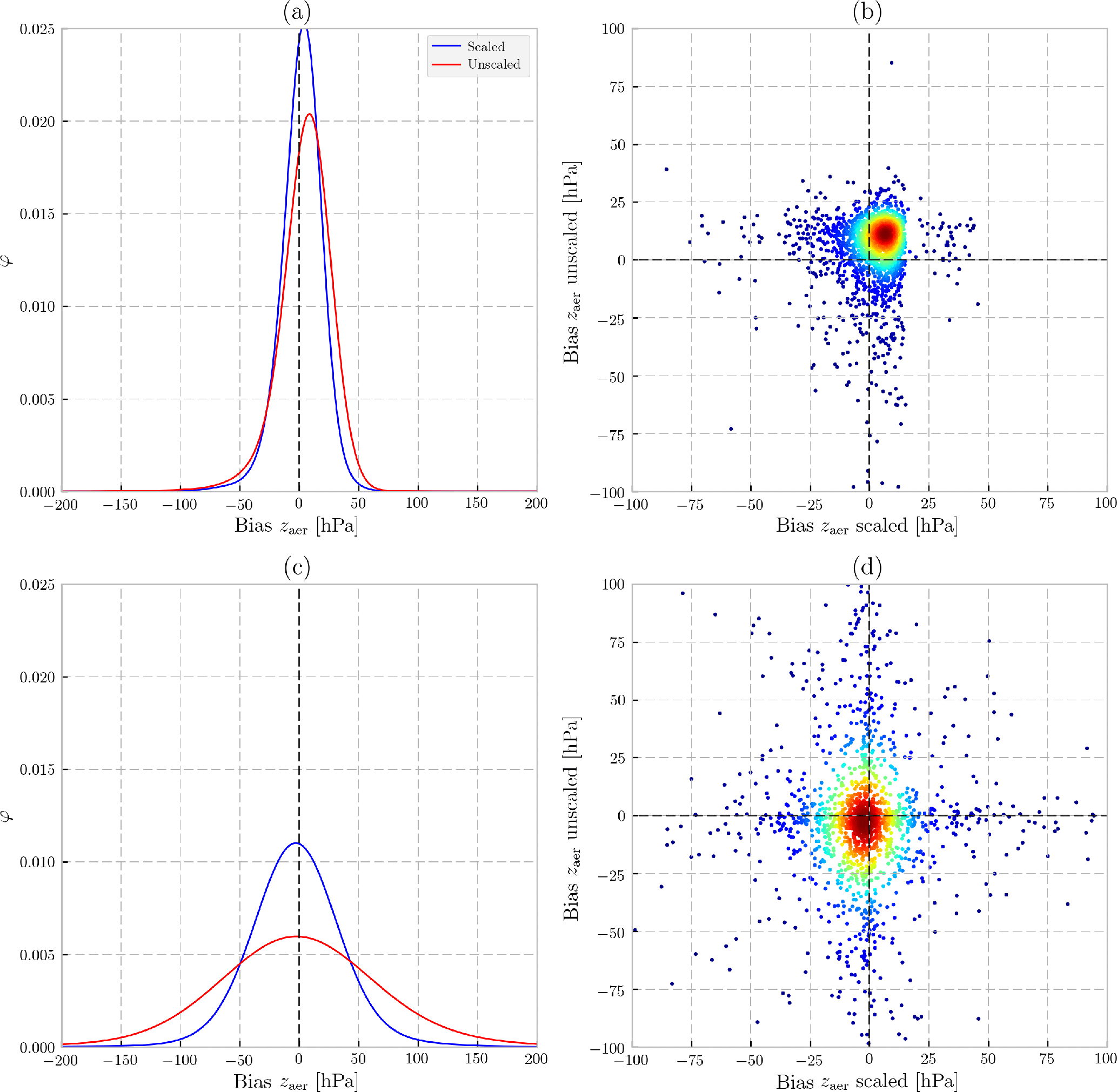
Figure 2 Biases in retrieved z_aer (in hPa) from synthetic measurements (2000 in total for each experiment) discussed in Sect. 4. The top row represents z_aer biases in the presence of a model error in the thickness of the aerosol layer. The bottom row represents z_aer biases in the presence of a model error in A_s. (a, c) Probability distribution function φ of retrieval biases. Blue line represents results from the dynamic scaling method, and the red line represents those for the formal approach. (b, d) 2-D density plot showing the distribution of biases (density ranges from high in red to low in blue). The x axis represents biases from the dynamic scaling method, whereas the y axis represents biases from the formal approach.

A spectrometer's detector pixel (in the spectral dimension) that contains a higher concentration of oxygen absorption lines receives less number of photons, in comparison to spectral points that contain fewer or no absorption lines. As a result of this, the relative error at these spectral points is larger, resulting in a lower signal-to-noise ratio (SNR). The expression of noise in the S_ϵ matrix at each spectral point is hence dependent on the average absorption line strength within a spectral point. When the surface becomes brighter (e.g. over land), the number of photons travelling from the surface to the detector increases heterogeneously, depending on many contributing factors such as oxygen absorption line strength, AOT, ALH and other atmospheric properties. In principle, however, the increase in signal for detector pixels with low oxygen absorption cross section is much higher than that for detector pixels with a high oxygen absorption cross section. This will be reflected in the S_ϵ matrix, which will (for example) rank measurements in the continuum higher than those in the deepest part of the absorption band.

If the information on ALH is derived from absorption by oxygen, this design of the ${\mathbf{S}}_{\mathit{ϵ}}^{-\mathrm{1}}$ matrix does not encourage an accurate ALH retrieval. From a WLSE standpoint, the consequences of an increase in the number of photons in the TOA reflectance that travel to the surface can be quite significant, some of which are reported in Fig. 7 of Nanda et al. (2018). A possible avenue through which the ${\mathbf{S}}_{\mathit{ϵ}}^{-\mathrm{1}}$ matrix can be improved involves its dynamical manipulation. The manipulation proposed in this paper has been termed the dynamic scaling method. The next section elucidates this method with a comparative analysis against the formal inverse method, henceforth called the formal approach, and is presented further on in this paper.

3 The dynamic scaling method

Table 1 Input parameters for synthetic experiments.

The dynamic scaling method identifies favourable spectral points for ALH retrieval by first identifying spectral points that are the least favourable. The noise is increased at these unfavourable points while keeping the noise at the other points unchanged. These favourable and unfavourable spectral points are identified using a class of vectors known as modifying vectors (with the symbol 𝓜 and length equal to the number of spectral points).

To identify the unfavourable spectral points at which the measurement noise is to be modified, a modifying vector ${\mathcal{M}}_{A_{\mathrm{s}}/z_{\text{aer}}}$ is proposed as

$$\begin{array}{}\text{(6)}& {\displaystyle }{\displaystyle }{\mathcal{M}}_{A_{\mathrm{s}}/z_{\text{aer}}}\left({\mathit{\lambda }}_i\right)={\displaystyle \frac{{\mathbf{K}}_{A_{\mathrm{s}}}\left({\mathit{\lambda }}_i\right)}{{\mathbf{K}}_{z_{\text{aer}}}\left({\mathit{\lambda }}_i\right)}}\left[\text{hPa}\right],\end{array}$$

where ${\mathbf{K}}_{A_{\mathrm{s}}}\left({\mathit{\lambda }}_i\right)$ is the derivative of the TOA reflectance with respect to surface reflectance at the ith index of the spectral point on the detector, and ${\mathbf{K}}_{z_{\text{aer}}}\left({\mathit{\lambda }}_i\right)$ is the same for z_aer. In principle, the ratio of ${\mathbf{K}}_{A_{\mathrm{s}}}$ and ${\mathbf{K}}_{z_{\text{aer}}}$ is used as an identification tool since our primary retrieval parameter is z_aer, which reduces its information as A_s increases. This opposing nature is discussed by Nanda et al. (2018) (Figs. 3 and 4 in their paper), where they show an anti-correlation in the sensitivity of τ and z_aer in the atmospheric path contribution and surface contribution to the TOA reflectance. A large value in ${\mathcal{M}}_{A_{\mathrm{s}}/z_{\text{aer}}}\left({\mathit{\lambda }}_i\right)$ represents spectral points in the measurement with more sensitivity to A_s than to z_aer. The motivation for choosing derivatives as the means for modification is also partly motivated from the fact that they are scene-dependent parameters, which makes each modification unique to the scene.

Spectral points with a ${\mathcal{M}}_{A_{\mathrm{s}}/z_{\text{aer}}}\left({\mathit{\lambda }}_i\right)$ higher than a specific threshold value should have a limited representation in the estimation – these are the unfavourable spectral points. We define this threshold as the modifying threshold (𝒯), which is the 20th percentile value of ${\mathcal{M}}_{A_{\mathrm{s}}/z_{\text{aer}}}$. The threshold value set in our method has been chosen in a way to avoid scaling the deeper parts of the R and P branches in the A band. The choice of thresholding remains configurable to the user of this method, based on their requirements – in our case we have chosen to use a static rule for deciding the value of 𝒯, but this could also be made dynamic. An example of the shape of ${\mathcal{M}}_{A_{\mathrm{s}}/z_{\text{aer}}}$ is provided in Fig. 1 (top row).

The reason for increasing the noise at specific unfavourable spectral points is to increase the value of S_ϵ at these points. With a higher S_ϵ value, the ${\mathbf{S}}_{\mathit{ϵ}}^{-\mathrm{1}}$ value will be lower, and hence that spectral point will have a lower weight in the estimation. In principle, this is equivalent to artificially increasing noise of measurements that contain less sensitivity to ALH. To do this, the modified SNR (denoted by SNR_𝓜) is defined as

$$\begin{array}{}\text{(7)}& {\displaystyle }{\displaystyle }{\text{SNR}}_{\mathcal{M}}\left({\mathit{\lambda }}_i\right)=\left\{\begin{array}{l}\text{SNR}\left({\mathit{\lambda }}_i\right)\text{if }{\mathcal{M}}_{A_{\mathrm{s}}/z_{\text{aer}}}\left({\mathit{\lambda }}_i\right)<\mathcal{T}\\ \text{SNR}\left({\mathit{\lambda }}_i\right)/{\mathcal{M}}_{A_{\mathrm{s}}/\mathit{\tau }}\left({\mathit{\lambda }}_i\right)\text{otherwise},\end{array}\right.\end{array}$$

where ${\mathcal{M}}_{A_{\mathrm{s}}/\mathit{\tau }}\left({\mathit{\lambda }}_i\right)$ (belonging to the class of modifying vectors) is defined as the ratio between the derivative of the TOA reflectance with respect to the surface (${\mathbf{K}}_{A_{\mathrm{s}}}\left({\mathit{\lambda }}_i\right)$) and with respect to AOT (τ) at 760 nm (K_τ(λ_i))

$$\begin{array}{}\text{(8)}& {\displaystyle }{\displaystyle }{\mathcal{M}}_{A_{\mathrm{s}}/\mathit{\tau }}\left({\mathit{\lambda }}_i\right)={\displaystyle \frac{{\mathbf{K}}_{A_{\mathrm{s}}}\left({\mathit{\lambda }}_i\right)}{{\mathbf{K}}_{\mathit{\tau }}\left({\mathit{\lambda }}_i\right)}}[-].\end{array}$$

The choice of modifying the SNR based on ${\mathcal{M}}_{A_{\mathrm{s}}/\mathit{\tau }}$ arises from the fact that the amount of contribution by the aerosol layer to the TOA reflectance depends on its optical thickness. In this case, we are interested in how much this contribution fares against the contribution from the surface. Information on both of these contributions can be inferred from the ratio of ${\mathbf{K}}_{A_{\mathrm{s}}}$ and K_τ, which have comparatively similar shapes. If the measurement of a spectral pixel i is more sensitive to A_s, ${\mathcal{M}}_{A_{\mathrm{s}}/\mathit{\tau }}\left({\mathit{\lambda }}_i\right)$ will be larger, and hence the noise at i will be increased, following Eq. (7).

To run a retrieval using the dynamic scaling method, the derivatives of the reflectance with respect to A_s, z_aer and τ at 760 nm are calculated first, followed by the modification of SNR according to Eq. (7). The state vector parameters τ and z_aer are then estimated using SNR_𝓜. Users of this method may choose to scale the measurement error covariance matrix at each iteration, since the derivatives change at each iteration. Nevertheless, we have chosen to do it semi-statically since the measurement error covariance matrix is a static matrix throughout every iteration.

Examples of modifying vectors and SNR_𝓜 are provided in Fig. 1 (bottom row), which shows the robustness of the method in scaling the SNR for different surfaces. The spectra generated in the figure represents two scenes with identical atmospheric parameters, solar and satellite geometries, but different A_s. ${\mathcal{M}}_{A_{\mathrm{s}}/z_{\text{aer}}}$, 𝒯 and ${\mathcal{M}}_{A_{\mathrm{s}}/\mathit{\tau }}$ for different surfaces are different – this is important, since overscaling the SNR can force the retrieval to rank the measurements of photons travelling from the upper parts of the atmosphere higher while ignoring those from the lower parts of the atmosphere. This is why the modifying vector ${\mathcal{M}}_{A_{\mathrm{s}}/\mathit{\tau }}$ is chosen as a dynamically scene-dependent parameter (according to Eq. 8), such that the scaling is large when A_s is large (Fig. 1, mid row). In the next section, the dynamic scaling method is demonstrated and compared to the formal approach (which is the unscaled OE method) for synthetically generated spectra.

4 Sensitivity analyses

To demonstrate the dynamic scaling method, synthetic spectra are generated for randomly varying values in z_aer, τ, solar-satellite geometry (θ, θ₀ and ϕ−ϕ₀), and A_s, while keeping other parameters constant. Noise is not added to the synthetic spectra. This method of randomly generating model parameters for generating synthetic spectra gives a broad picture of the method's behaviour. Table 1 provides a brief overview of the input model parameters chosen to generate these spectra. An error is introduced in the forward model during retrieval, and the bias in z_aer (defined as retrieved – true) is used to assess the retrieval. The a priori z_aer and τ are set at 825 hPa and true τ, respectively. While there are many possible sources of errors, this paper presents two kinds of errors: (a) error in the thickness of the aerosol layer, and (b) error in the surface albedo database. A reason for limiting the retrieval experiment scope to these two errors in the atmospheric part of the forward model is due to the fact that they are one of the more common contributors to retrieval biases. In real cases, aerosol layers may not be concentrated in a single layer of 50 hPa thickness, and the true surface albedo may vary significantly (to the order of 10 % relative errors) from a monthly database of Lambertian equivalent reflectivity (LER) values depending on many parameters. In total, 2000 synthetic spectra are generated for each synthetic experiment and the parameters z_aer and τ are estimated using both the formal approach and the dynamic scaling method to be compared side by side. The results from analysing biases in retrieved z_aer are plotted in Fig. 2. Although the dynamic scaling method is specifically designed for land, retrievals over surfaces with a low A_s (less than 0.1) are also included.

Table 2 Results of the retrieval accuracy of z_aer from sensitivity analyses, split into two classes of A_s. The number of successful retrievals are reported in the “retrieved” column. Columns with the heading A are the locations of the peak of φ, representing the z_aer bias value with the highest frequency of occurrence. Those with B are the full-width at half maximum of φ, representing the spread of z_aer biases.

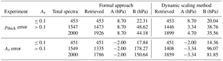
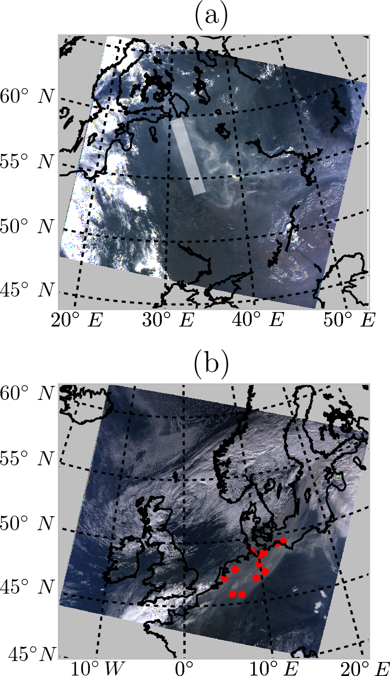
Figure 3 MODIS Terra images of the two test cases. (a) MODIS RGB composite on 08:50 UTC, 8 August 2010 of the 2010 Russian wildfires. The white line represents an approximation of CALIPSO's ground track. (b) Portugal wildfire plume observed by MODIS Terra on 11:00 UTC over western Europe on 17 October 2017. Blue dots represent 12 ceilometer locations.

4.1 Error in aerosol layer thickness

The synthetic spectra generated assume an aerosol layer thickness (p_thick) of 100 hPa, whereas the retrieval forward model assumes a 50 hPa thickness. For simplicity, a PDF (denoted by φ) of the biases of retrieved z_aer is calculated, the peak of which represents the value of maximum frequency of occurrence, and the full-width at half maximum, which represents the spread.

In comparison with the formal approach (Fig. 2a), the peak of φ for the dynamic scaling method is closer to 0 hPa and has a larger magnitude (Table 2). The retrieval biases for A_s≤0.1 and above 0.1 are indicative of the robustness of the dynamic scaling method in its scaling of the SNR (Table 2, p_thick bias row). For A_s≤0.1, the retrieval biases from both dynamic scaling and formal approach are almost identical. Splitting the results to τ≤2.0 and τ>2.0, it is observed that the dynamic scaling method reduces retrieval biases of z_aer by 40 % relative to those from the formal approach for high aerosol loads and about 11.5 % for low aerosol loads. This is because a scene containing low aerosols allow for more interactions between photons and the surface, which results in ALH retrievals being biased closer to the surface. The dynamic scaling method ameliorates this behaviour by reducing the sensitivity of the retrieval algorithm to these photons. The formal approach retrieves 27 more pixels than the dynamic scaling method for A_s>0.1. An observation to note is that there are instances where even the dynamic scaling method can result in large retrieval biases (Fig. 2b). Generally, however, the dynamic scaling method is shown to reduce retrieval biases in the presence of model errors in the aerosol layer thickness.

4.2 Error in surface albedo database

To generate errors in surface albedo, randomly varying relative errors (with respect to the true surface albedo in the synthetic spectra) ranging between −10 and 10 % were introduced to the retrieval forward model. The results heavily favour the dynamic scaling method, which shows a significant improvement in retrieval behaviour over the formal method. The dynamic scaling method retrieves 73 more pixels than the formal approach (Table 2, A_s error row) while also having a much smaller spread of retrieval biases around the peak (Fig. 2c). For A_s≤0.1, the dynamic scaling method and the formal approach are almost identical, with the dynamic scaling method having a smaller spread. For A_s>0.1, however, the dynamic scaling method improves the spread of the retrieval biases significantly. The mean biases for the dynamic scaling approach are slightly larger than those for the formal approach, and the spread of retrieval biases in Fig. 2d indicates that the dynamic scaling method does not necessarily improve retrieval biases for all cases. However, the dynamic scaling method improves convergence from 89.3 to 92.3 % and reduces bias for 86.4 % of the cases.

The analysis of retrieval biases from the synthetic sensitivity analyses are very encouraging for the dynamic scaling method. The method has shown significant improvements for A_s>0.1 (at 760 nm) in the presence of two very relevant model errors. The fact that the dynamic scaling method is almost identical to the formal approach for A_s≤0.1 reaffirms the design of the modifying vector ${\mathcal{M}}_{A_{\mathrm{s}}/\mathit{\tau }}$, which is intended to modify the SNR only if the modification is necessary. A similar split of results for τ≤2.0 and τ>2.0 reveals that the dynamic scaling method is almost similar to the formal approach for low values of τ, and only results in significant improvements if the scene contains sufficient aerosols. Relative to z_aer biases from the formal approach, the biases from the dynamic scaling are reduced by 53 % for τ>2.0 and are practically the same for τ≤2.0. The success of the dynamic scaling method in a synthetic environment also confirms the fact that the design of the ${\mathbf{S}}_{\mathit{ϵ}}^{-\mathrm{1}}$ plays an important role in the biases of the retrieved z_aer. The next section applies the dynamic scaling method to measured spectra from GOME-2A and GOME-2B instruments over aerosol plumes from forest fire events in Europe.

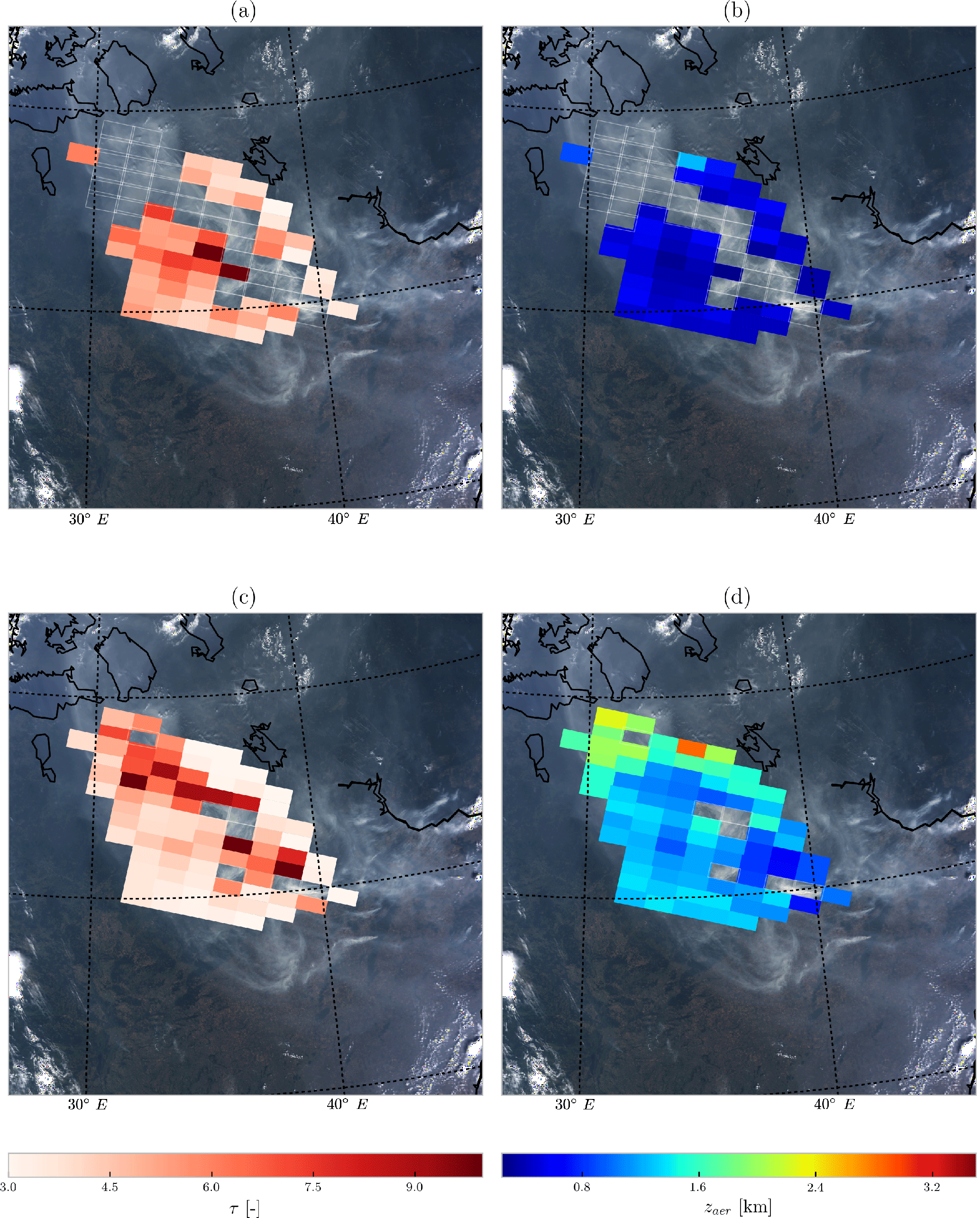
Figure 4 Results from processing 85 GOME-2A pixels over Russia on 8 August 2010 using the formal approach and the dynamic scaling method. Empty GOME-2A pixels with a white border represent non-convergences. (a) Fitted τ at 760 nm from the formal approach. (b) Retrieved z_aer from the formal approach. (c) Fitted τ at 760 nm from the dynamic scaling method. (d) Retrieved z_aer from the dynamic scaling method. The background image for all plots is a subset of the MODIS Terra image in Fig. 3a.

5 Application to GOME-2 data

The GOME-2 instrument is a part of an operational mission by the European Organization for the Exploitation of Meteorological Satellites (EUMETSAT) to monitor trace gases and aerosols in the atmosphere. It is a spectrometer with an across-track scanning mirror that projects the TOA Earth radiance and solar irradiance through a prism on a grating to get information in the ultraviolet, visible and the near-infrared regions of the electromagnetic spectrum. In the oxygen A band, the spectral sampling interval is typically about 0.20 nm and the FWHM is 0.50 nm (Munro et al., 2016). The GOME-2 instrument is designed to have a footprint size of 80 km×40 km in the oxygen A band. The instrument also measures the linear polarization of Earth radiance, which is important for correcting the measured signal to calculate the reflectance accurately.

In this section, measured spectra from the GOME-2A instrument on board the Metop-A satellite over Russian wildfires on 8 August 2010 (Fig. 3a) and the Portuguese fire plume are used with the GOME-2B instrument on board the MetOp-B satellite on 17 October 2017 over western Europe (Fig. 3b). The formal OE method is compared to the dynamic scaling method by using space-based and ground-based validation data. The noise spectrum is derived from the GOME-2 level 1-b product, which is a combination of the systematic and random error components of the measurements (EUMETSAT, 2014).

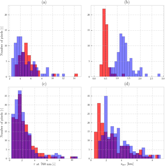
Figure 5 Histograms of fitted aerosol optical thickness (τ, left column) and aerosol layer height (z_aer, right column) from GOME-2A and GOME-2B pixels. Histograms in red are retrievals from the formal approach and the histograms in blue are results from the dynamic scaling method. (a) Fitted τ from the GOME-2A pixels over the 8 August 2010 wildfire plume over Russian. (b) Retrieved z_aer from the GOME-2A pixels over the 8 August 2010 wildfire plume over Russian. (c) Fitted τ from the GOME-2B pixels over the 17 October 2017 wildfire plume over western Europe. (d) Retrieved z_aer from the GOME-2B pixels over the 17 October 2017 wildfire plume over western Europe. The axes are adjusted for each plot.

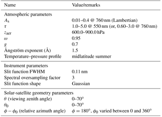
Auxiliary information required for these retrievals are meteorological data, surface albedo, and a priori values for the optimal estimation (Table 3). The meteorological data required are temperature–pressure profiles and the surface pressure, derived from the ERA-Interim database from Dee et al. (2011). These meteorological parameters are available on regular space ($\mathrm{1}{}^{\circ }\times \mathrm{1}{}^{\circ }$ spatial resolution) and time grids, and require interpolation to the satellite pixel's coordinates and time of record. This interpolation is done using the nearest-neighbour algorithm. The surface albedo database is derived from Tilstra et al. (2017) version 2.1, which has a resolution of $\mathrm{0.25}{}^{\circ }\times \mathrm{0.25}{}^{\circ }$, derived from the GOME-2A instrument. The surface LER is chosen as the median of all LER database pixels intersecting the GOME-2 instrument pixel at wavelengths 758 and 772 nm with linear interpolation used for calculating LER values at intermediate wavelengths. Algorithm settings are detailed in Table 3. The test cases chosen in this paper are relatively cloud-free but not fully.

Tilstra et al. (2017)Alexander et al. (2016)

Table 3 Input data and algorithm set-up for retrieving aerosol properties from GOME-2 measurements in the oxygen A band.

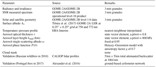
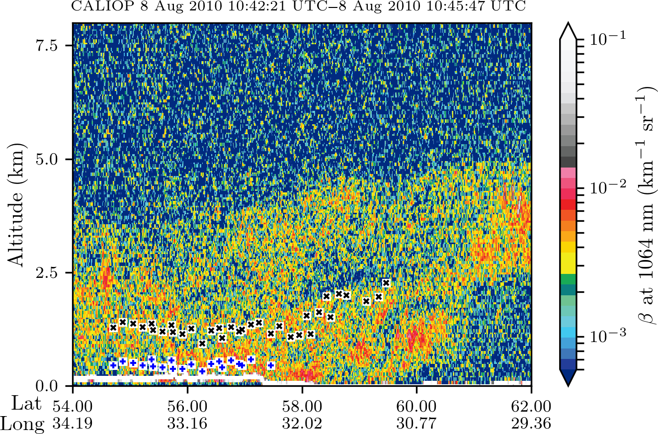
Figure 6 GOME-2A-derived aerosol layer heights co-located within 100 km to the CALIPSO ground track (using great circle distance), plotted over attenuated backscatter (β) of the CALIOP lidar at 1064 nm. The blue and black markers in white squares represent converged ALH from the formal approach and the dynamic scaling method, respectively.

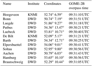
For validation, atmospheric lidar data from satellite and ground-based instruments are chosen. For the 2010 Russian wildfires, the lidar-attenuated backscatter at 1064 nm from the CALIOP instrument (Cloud-Aerosol LIdar with Orthogonal Polarization) are used on board NASA's CALIPSO (Cloud-Aerosol Lidar and Infrared Pathfinder Satellite Observations) mission. These data have a very good representation of the scattering ability of clouds and aerosols in the atmosphere at a vertical resolution of 60 m and a horizontal resolution of 5 km. For the 2010 Russian wildfires, the CALIPSO overpass is at 10:45 UTC. All GOME-2A pixels co-located within a 100 km vicinity of a CALIOP profile are considered for validation. For the 17 October 2017 Portugal fire plume over western Europe, ground-based ceilometer data are used for validation (Table 4). These ceilometers are a part of the ALC (Automated Lidars and Ceilometers) network of the E-PROFILE observation programme in the framework of the European Meteorological Services Network (EUMETNET). The parameter used for validation is the uncalibrated raw backscatter profile, since the paper focuses on qualitatively assessing the aerosol height retrievals with the lidar backscatter profiles. Lidar profiles within an hour of the satellite instrument overpass time are averaged into a single averaged profile in order to reduce noise. These lidars have a vertical range of approximately 15 m and record data at a very high temporal resolution, nominally every 6 s (Alexander et al., 2016). Although CALIOP data is available for the plume over western Europe for October 2017, CALIPSO does not have as good a co-location (both spatially and temporally) in comparison to the ceilometers.

Table 4 Ceilometer stations in western Europe used for validating the retrieved z_aer from GOME-2B for plumes from the 17 October 2017 Portugal wildfires.

5.1 Russian wildfires on 8 August 2010

The wildfire plumes in and around Moscow on 8 August 2010 are chosen as the test case for the dynamic scaling method. Anti-cyclonic conditions on this day meant that the region of interest was predominantly cloud-free. This case is the same as analysed in Nanda et al. (2018) (but with a smaller pixel selection to only focus on the plumes), with the exception that the study presented in the current paper uses a more recent version of the surface LER product from Tilstra et al. (2017) with a larger amount of GOME-2A data incorporated into its creation. The inclusion of this more recent LER database has slightly improved the results from the formal approach but not significantly. A MODIS Terra image taken over the region on the same day (Fig. 3a) shows that the plume, although thick, is non-homogeneously distributed in the scene, since the sources of fire are very close to the region of interest described in the test case. There are 85 GOME-2A pixels over the primary biomass burning plume that are considered for retrieving AOT and ALH. During the iterations, if the inverse method estimates non-physical state vector values (such as an aerosol layer below the surface and a negative AOT or a cloud-like optical thickness) twice in a row, the retrieval is stopped and is said to have failed to converge. The algorithm also provides an upper cap of 12 iterations, beyond which the retrieval is also labelled to have failed to converge.

On applying the formal ALH retrieval approach, 49 pixels converge and 36 pixels do not converge to a solution (Fig. 4a and b). The fitted AOT values are in excess of 6.0 in many cases – on average, the fitted AOT is 5.34 with a SD of 1.87 (Fig. 5a, red). These values are too high – the AErosol RObotic NETwork (AERONET) station in Moscow observed, on the same day, values between 1.0 at 870 nm and 1.5 at 675 nm between 09:00 and 10:00 UTC, whereas our retrieval estimates an AOT of 6.60 at 760 nm over Moscow using dynamic scaling. The distribution of fitted τ appears to be spatially inconsistent with the aerosol plume observed by MODIS Terra (Fig. 4a). The formal approach misses the primary biomass burning aerosol plume. The average retrieved height of the plume is 0.5 km above the ground, with a SD of 0.15 km (Fig. 5b, red histogram). Realistically, one can expect aerosols this close to the surface, especially if the boundary layer captures much of the pollution. However, aerosol-corrected boundary layer height modelled by Péré et al. (2014) for the same day over Moscow shows that the atmospheric boundary layer is approximately around 1.5–2.0 km altitude. Comparing the retrieval to co-located CALIPSO data in Fig. 6 (blue markers), there are aerosols observed up to 4 km altitude, possibly in a multi-layered structure. Based on the CALIPSO observations and the modelled height of the atmospheric boundary layer, the retrieved ALH seems to be biased low in the atmosphere; thus it is too close to the surface. These results are summarized in Table 5.

Table 5 Retrieval results from GOME-2 experiments. Columns marked with A, B, C and D are mean retrieved z_aer (km), SD of retrieved z_aer (km), mean fitted τ and SD of the fitted τ, respectively. n_total represents the total number of pixels in the scene, and n_ret represents the number of retrieved pixels. A_s avg represents the average surface albedo of the scene.

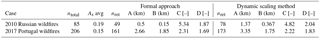
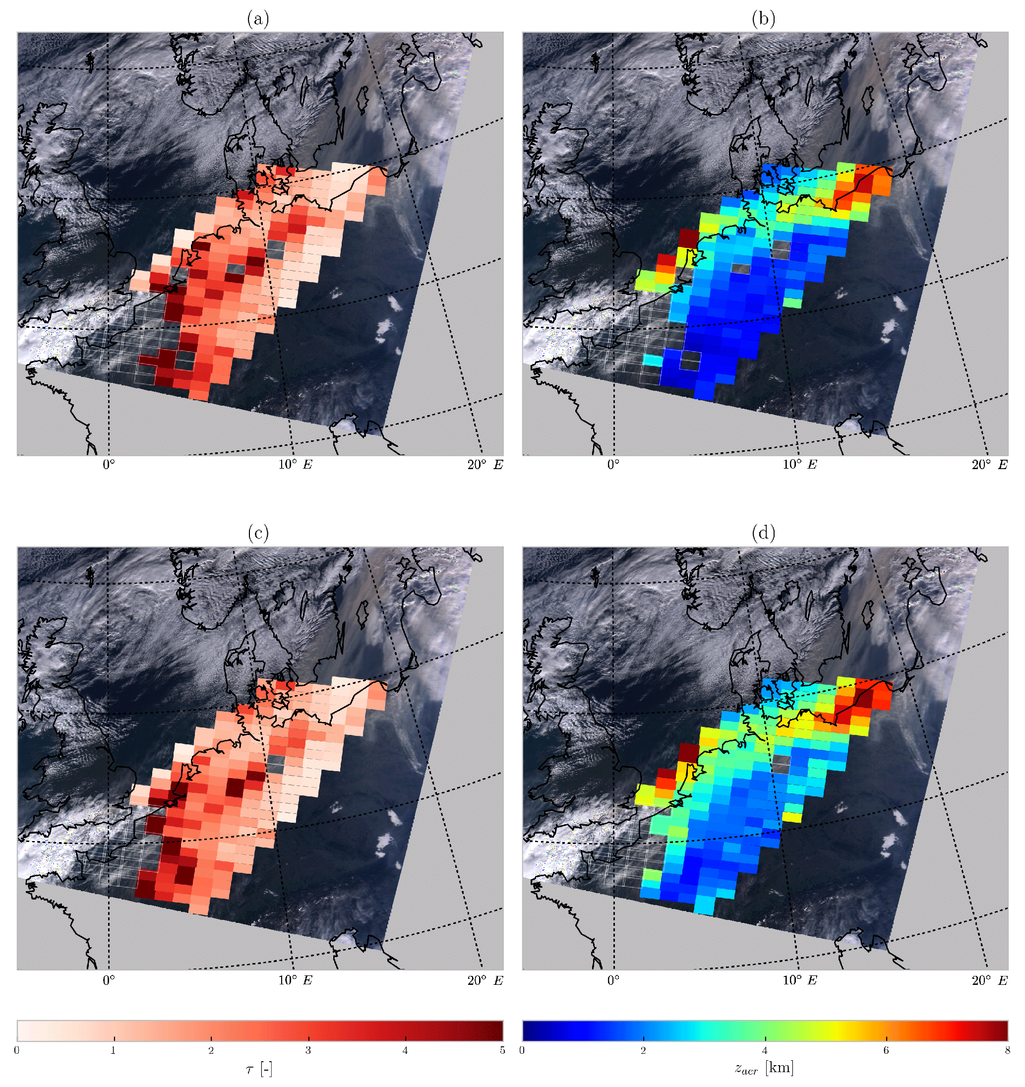
Figure 7 Results from processing 206 GOME-2B pixels over western Europe using the formal approach and the dynamic scaling method. Empty GOME-2B pixels with a white border represent non-convergences. (a) Fitted τ at 760 nm from the formal approach. (b) Retrieved z_aer from the formal approach. (c) Fitted τ at 760 nm from the dynamic scaling method. (d) Retrieved z_aer from the dynamic scaling method. The background image is a subset of the MODIS Terra image in Fig. 3b.

Applying the dynamic scaling method to the same scenario, we observe an increase in the number of convergences to 78 pixels out of the 85 chosen (60 % increase compared to the formal approach), as shown in Fig. 4c and d. The fitted AOT is approximately 4.82, with a SD of 2.04 (Fig. 5a, blue histogram). While these fitted AOT values are still high in the scene, the spatial distribution is consistent with the biomass burning plume seen by MODIS (Fig. 4c). The retrieved ALH is, on average, 1.37 km, with a SD of 0.367 km (Fig. 5b, blue histogram). Looking at CALIPSO data, this value appears to be more realistic for the biomass burning plume (Fig. 6, black markers), as the aerosol particles are located farther away from the surface.

5.2 Portugal fire plume over western Europe on 17 October 2017

The October 2017 Portugal wildfires began in the third week of October. On 16 October, the hurricane Ophelia made landfall over Ireland as a midlatitude cyclone. Due to the cyclonic conditions the forest fire aerosol plumes were pulled from Portugal into western Europe along with Saharan desert dust (CAMS, 2017), which was observed the next day (Fig. 3b). The aerosol plumes from these fires are different from the aerosol plumes observed in the 2010 Russian wildfires, primarily because our region of interest is farther away from the fires; the plume over western Europe appears to be more homogeneous. The GOME-2B overpass on 17 October 2017 is approximately around 09:30 UTC, and the MODIS image in Fig. 3b is approximately around 11:00 UTC. Although some of these GOME-2B pixels may be cloud contaminated, our retrieval assumes cloud-free conditions. This assumption can result in large values in retrieved aerosol heights and fitted optical thicknesses. 206 GOME-2B pixels are chosen for this study. On average, the LER of this scene from the 2017 fires is 0.15 at 760 nm, whereas that for the 2010 fires is 0.19; see Table 5.

Out of the 206 pixels, 161 pixels converge to a solution from the formal approach (Fig. 7a and b). The fitted τ at 760 nm is on average 2.31, with a SD of 1.69 (Fig. 5c, red histogram). Typical fitted τ over the plume seems to be around 3.0, which is too high a value for this case, since it disagrees with AERONET measurements, which show AOT values approximately between 2.0 and 1.0 at 675 and 870 nm over Lille during the GOME-2B overpass time. The retrieved z_aer is, on average, approximately 2.66 km from the ground with a SD of 1.85 km (Fig. 5d, red histogram). Many of the pixels that do not converge seem to be cloudy (the bottom corner of the GOME-2B pixels, Fig. 7a). The dynamic scaling method increases the number of convergences to 173 pixels (Fig. 7c and d). On average, this method retrieves an ALH of 3.35 km, with a SD of 1.75 km (Fig. 5d, blue histogram). The average AOT at 760 nm fitted is 2.22 with a SD of 1.83 (Fig. 5c, blue histogram).

Comparing the retrieved z_aer is to profiles from a ground-based ceilometer in De Bilt, the Netherlands (Fig. 8a, black profile), the first observation is that the dynamic scaling method seems to retrieve a height that is more representative of the top of the aerosol layer, whereas the formal approach retrieves a more realistic aerosol height that is more or less at the centroid of the elevated layer's profile. It is, however, important to note that pulses from ceilometers are weak and tend to get attenuated beyond the bottom of the aerosol layer. Because of this, layers above these can appear as weak backscatter even though they may not be. A radiosonde profile of the relative humidity reveals the presence of an atmospheric layer that extends well beyond the altitude range from where the lidar backscatter becomes progressively weaker. This profile also shows the presence of a layer at the 200–400 hPa pressure levels, coinciding with a weak attenuated backscattered signal observed by the ceilometer in the same atmospheric level. A look into back trajectories, calculated using the TRAJKS model described in Stohl et al. (2001), shows that the pressure levels between 800 and 600 hPa (at De Bilt) likely contains aerosols carried from Portugal to De Bilt (Fig. 8b). The back trajectory of air mass at 250 hPa also passes through this peninsula but may not contain biomass burning aerosols since the layer at this atmospheric level does not mix with the lower level (according to the TRAJKS calculations). Following this, we have compared the retrieved z_aer from both methods to backscatter profiles from other ceilometer stations, reported in Fig. 9. In general, while both the dynamic scaling method and the formal approach retrieve z_aer values that fall within the aerosol plumes, the dynamic scaling method retrieves heights that are slightly greater. This has to do with our conclusions from Fig. 8.

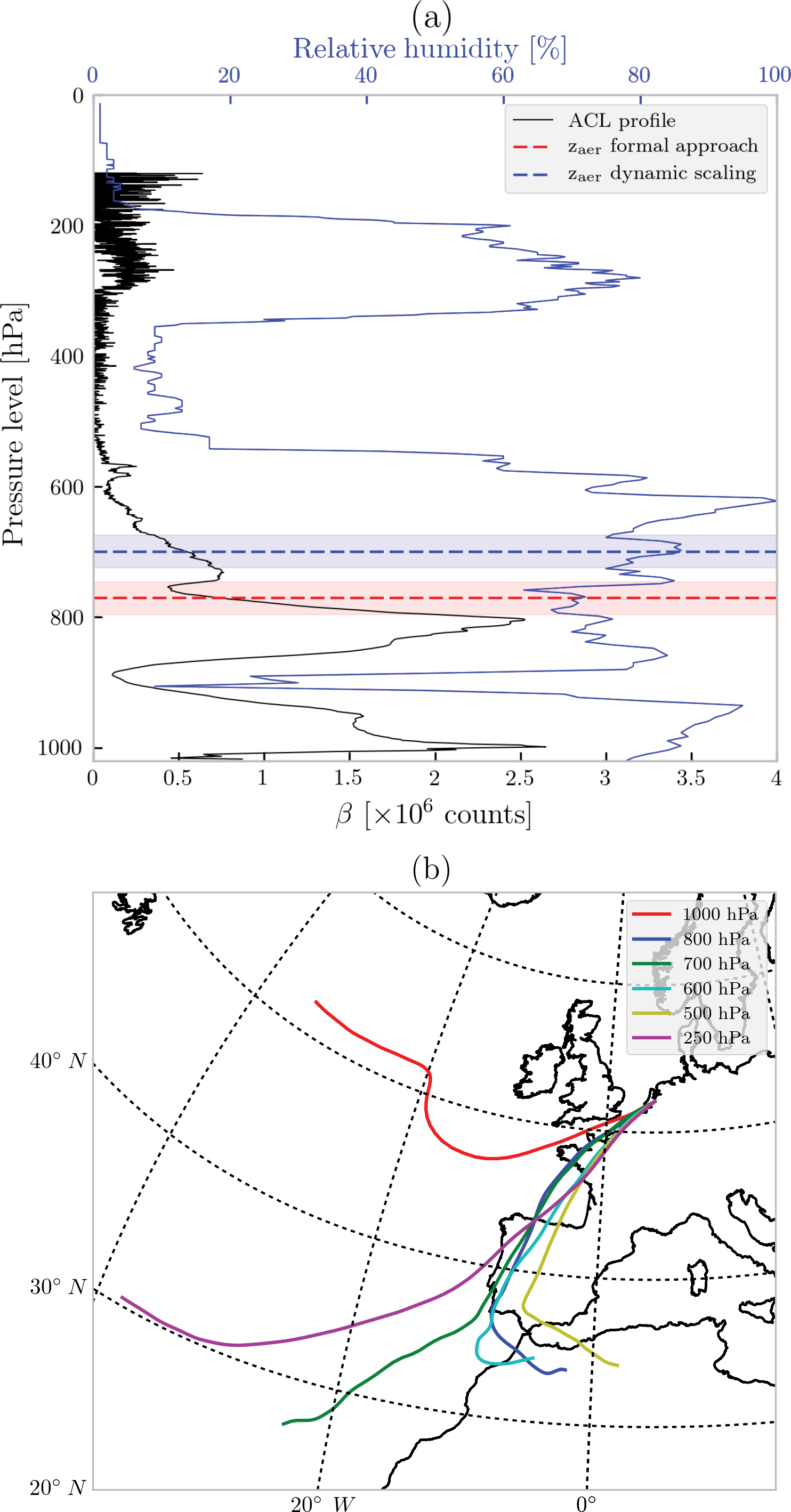
Figure 8 (a) Radiosonde profile of relative humidity (blue), plotted alongside an averaged raw attenuated backscatter profile (black) from the ceilometer at De Bilt, the Netherlands. Both profiles are approximately around 13:00 UTC. The red and blue dashed lines represent retrieved aerosol layer height using the formal approach and the dynamic scaling method, respectively. The red- and blue-shaded boxes represent the aerosol layer from the respective retrieval methods. (b) Back trajectories calculated for 17 October 2017 at 13:00 UTC with the end point at De Bilt, and the sources going back to 3 days.

Figure 9 Validation of the retrieved aerosol layer height over western Europe from ceilometers located in the Netherlands and Germany from the CEILONET and DWD networks. The black lines represent averaged ceilometer profiles of acquisitions 1 h before and after the GOME-2B overpass over each location (600 profiles). The profiles are uncalibrated raw attenuated backscatter β as a function of lidar range (km). The grey-shaded region represents the SD of the profiles used to create the averaged profile. The red and blue dashed line represents retrieved aerosol layer height using the formal approach and the dynamic scaling method, respectively. The red- and blue-shaded boxes represent the aerosol layer from the respective retrieval methods.

The LER of a scene tells us which surface is brighter. In this case, the surface in the 2010 Russian fires was brighter than that in the 2017 western Europe case. The values of the modifying vectors ${\mathcal{M}}_{A_{\mathrm{s}}/z_{\text{aer}}}$ and ${\mathcal{M}}_{A_{\mathrm{s}}/\mathit{\tau }}$ over the two different scenes, however, can tell us the influence of the surface on the measurements itself, since these parameters are a direct comparison of the sensitivity of the measurement to aerosol properties and surface albedo. On average, ${\mathcal{M}}_{A_{\mathrm{s}}/z_{\text{aer}}}$ and ${\mathcal{M}}_{A_{\mathrm{s}}/\mathit{\tau }}$ in the 2010 Russian wildfires are much larger in comparison to the same for the 2017 Portugal fire plume over western Europe (Fig. 10). This suggests that backscatter from the surface for the 2010 Russian wildfires plays a bigger role in the measurements observed by the GOME-2 instrument. The dynamic scaling method is hence effectively able to apply a wavelength-dependent scaling of the SNR by relying on scene-dependent parameters. If the modifying vector ${\mathcal{M}}_{A_{\mathrm{s}}/\mathit{\tau }}$ is very low, aerosol properties retrieved from the dynamic scaling method will be approximately equal to the same from the formal approach. This is an example of the robustness of the method – the SNR should only be scaled when there is a need for it to be scaled.

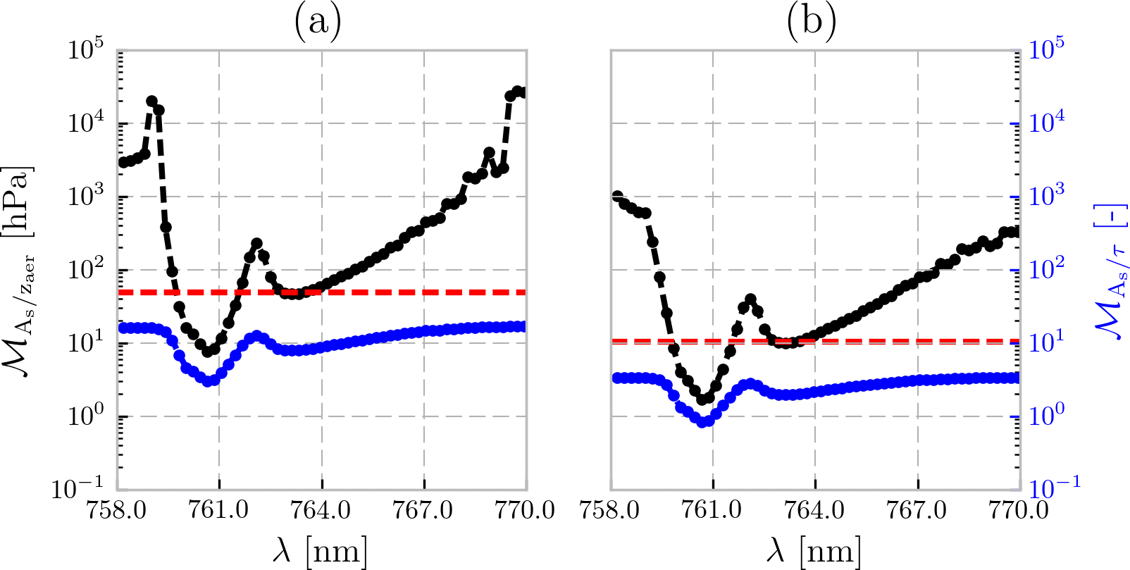
Figure 10 A comparison of the calculated matrices in the dynamic scaling method for all chosen GOME-2 pixels as a function of wavelength calculated for (a) the 2010 Russian wildfires and (b) the 2017 Portugal wildfires. The black dotted line is the averaged modifying vector ${\mathcal{M}}_{A_{\mathrm{s}}/z_{\text{aer}}}$ (Eq. 6) and the blue line is the averaged modifying vector ${\mathcal{M}}_{A_{\mathrm{s}}/\mathit{\tau }}$ (Eq. 8) for all GOME-2 pixels chosen in each scene. The y axis on the left is the range of values for ${\mathcal{M}}_{A_{\mathrm{s}}/z_{\text{aer}}}$ and that on the right is for ${\mathcal{M}}_{A_{\mathrm{s}}/\mathit{\tau }}$. The red line is the averaged modifying threshold 𝒯, which is set at the 20th percentile of ${\mathcal{M}}_{A_{\mathrm{s}}/z_{\text{aer}}}$.

6 Conclusions

Inversion algorithms that retrieve aerosol properties from spectral measurements in the oxygen A band (between 758 and 770 nm) can face a lot of trouble over land. This is primarily because of the location of oxygen A band beyond the red edge, a wavelength region that diminishes the ability of vegetation to absorb solar radiation as wavelength increases. This is especially the case when retrieving aerosol layer height using optimal estimation and radiative transfer models, as observed from Nanda et al. (2018); Sanders and de Haan (2016) and Sanders et al. (2015).

The optimal estimation framework, an application of the weighted least squares technique, is designed to rank data points (in this case, spectral points in the measured TOA radiance and solar irradiance) higher when the SNR is higher, in order to reduce the influence of measurement error in the final retrieved solution. In the oxygen A band, these spectral points coincide with weak oxygen absorption cross sections, since low absorption equates to a high number of photons that can traverse through the atmospheric medium. Over oceans, due to its low albedo the number of photons that travel back from the surface are few. The signal recorded by satellites from an ocean scene hence predominantly arises from scattering and absorption by atmospheric species (in this case, aerosols). Over land, however, the number of photons that travel back from the surface increase dramatically. Due to this, the optimal estimation framework ranks spectral points representing photons that have travelled back from the surface higher than those from aerosol layers. This is the primary error source when it comes to biases in aerosol retrievals from oxygen A band measurements over land.

This paper introduces the dynamic scaling method, which is designed to retrieve ALH over bright surfaces from oxygen A band measurements. The core principle of this proposed improvement is the wavelength-dependent modification of the measurement error covariance matrix by the subsequent wavelength-dependent modification of the signal-to-noise ratio of the measured spectrum, in order to reduce its preference towards photons that interact with the surface. The modification uses the scene-dependent Jacobian matrix, which makes it robust. The dynamic scaling method is compared with a formal optimal estimation approach by retrieving ALH and AOT from synthetically generated spectra with randomly varied model parameters and model errors (that is, the forward models for simulation and retrieval have different model parameters). The results from the synthetic experiments generally favour the dynamic scaling method, which shows a significant improvement in the accuracy of retrieved ALH in the presence of errors in the assumed aerosol geometric thickness and the surface albedo (up to 10 % relative errors) in the model.

The dynamic scaling method is also demonstrated for real spectra by using GOME-2A and GOME-2B oxygen A band measurements of two separate wildfire incidences in Europe, one being the 8 August 2010 Russian wildfires and the other being the more recent 17 October 2017 Portugal wildfires. In the case of the 2010 Russian wildfires, the formal optimal estimation retrieval approach produces few convergences and misses out the primary biomass burning aerosol plume (as observed from a MODIS Terra image). The fitted AOT are unrealistically high and spatially inconsistent with the aerosol plume observed by MODIS Terra. Co-located CALIOP lidar profiles show that the retrieved ALH is biased low in the atmosphere, closer to the surface. The dynamic scaling method, on the other hand, increases the number of converged pixels by 60 % in comparison to the formal approach. The fitted AOT is still too high, but the spatial distribution of the AOT compared to same observed in the MODIS Terra image is consistent. The retrieved ALHs are also more realistic, as they are positioned close to the centroid of the CALIOP-backscatter-profile-describing aerosols. For the Portugal wildfire plume on 17 October 2017 over western Europe, the dynamic scaling method does not increase the number of convergences significantly. The dynamic scaling method retrieves ALHs that are only slightly higher and fits AOTs at values are slightly lower in comparison to those from the formal approach. The retrieved heights from both methods are compared to lidar profiles from the EUMETNET ACL network of ceilometers. The comparison shows that both methods retrieved heights that are within the profiles that could be associated with aerosol layers. Analysing a radiosonde profile of the relative humidity and calculated back trajectories, it is observed that the ceilometer profiles miss higher aerosol layers due to attenuation of the signal at lower atmospheric levels. This explains why the retrieved heights from the dynamic scaling method are slightly higher than the same from the formal approach.

In general, the dynamic scaling method improves the number of converged pixels. Between the two discussed cases, the dynamic scaling method provides a better improvement in the 2010 Russian wildfires case. This is primarily because the method is scene dependent. An important driver that determines the improvement of retrievals is the level at which the surface influences the TOA reflectance, which is jointly influenced by two parameters – the surface albedo and the AOT. The average surface albedo of the scene for the 2010 Russian wildfires was observed to be brighter than the same for the 2017 Portugal wildfires. This is a possible explanation for the differences in the performance of the dynamic scaling method for the two cases.

The fitted AOT is systematically lower for the dynamic scaling method in comparison to the formal approach. A part of this can be attributed to the reduction in the influence of spectral points in the measurement with a larger influence from the surface albedo. While this is expected, the method does not necessarily make the fitted AOT more realistic. It may well be the influence of assumptions in aerosol properties such as aerosol single-scattering albedo and the phase function. It could, however, also be that the method does not fully remove the influence of surface in the measured top-of-atmosphere reflectance signal. In any case, the dynamic scaling method improves the representation of the fitted AOT of the MODIS Terra observed smoke plume.

The dynamic scaling method is designed to modify the signal-to-noise ratio to an extent that is necessary and sufficient to reduce the influence that photons travelling from the surface back to the detector have on the weighted least squares estimate of aerosol properties. Using the Jacobian to dictate the preference of weight least squares for spectral points in the measurement makes the dynamic scaling method a robust, generally applicable retrieval set-up. Results from this paper are applicable to other algorithms using weighted least squares techniques to retrieve atmospheric properties from measurements of top-of-atmosphere reflectance in the oxygen A band over bright surfaces.