the Creative Commons Attribution 4.0 License.
the Creative Commons Attribution 4.0 License.
 | 20 Jul 2018
Estimation of turbulence dissipation rate and its variability from sonic anemometer and wind Doppler lidar during the XPIA field campaign
Nicola Bodini
Julie K. Lundquist
Rob K. Newsom
Despite turbulence being a fundamental transport process in the boundary layer, the capability of current numerical models to represent it is undermined by the limits of the adopted assumptions, notably that of local equilibrium. Here we leverage the potential of extensive observations in determining the variability in turbulence dissipation rate (ϵ). These observations can provide insights towards the understanding of the scales at which the major assumption of local equilibrium between generation and dissipation of turbulence is invalid. Typically, observations of ϵ require time- and labor-intensive measurements from sonic and/or hot-wire anemometers. We explore the capability of wind Doppler lidars to provide measurements of ϵ. We refine and extend an existing method to accommodate different atmospheric stability conditions. To validate our approach, we estimate ϵ from four wind Doppler lidars during the 3-month XPIA campaign at the Boulder Atmospheric Observatory (Colorado), and we assess the uncertainty of the proposed method by data intercomparison with sonic anemometer measurements of ϵ. Our analysis of this extensive dataset provides understanding of the climatology of turbulence dissipation over the course of the campaign. Further, the variability in ϵ with atmospheric stability, height, and wind speed is also assessed. Finally, we present how ϵ increases as nocturnal turbulence is generated during low-level jet events.
- Article
(9621 KB) - Full-text XML
-
Supplement
(1644 KB) - BibTeX
- EndNote


Turbulence within the atmospheric boundary layer is critically important to transfer heat, momentum and moisture between the surface and the upper atmosphere (Sobel and Neelin, 2006). Hence, global and regional models need an accurate representation of turbulence to produce precise atmospheric predictions of winds, temperature and moisture in the boundary layer. An accurate forecast of these quantities has a critical impact on a variety of socioeconomic activities, such as pollutant dispersion, air quality forecasting (Huang et al., 2013), and forest fire prediction and management (Coen et al., 2013). Wind energy production is also highly affected by turbulence in the boundary layer, as a lower power is generated when turbulence intensity is high (Wharton and Lundquist, 2012), and turbulence also reduces the lifetime of wind turbines (Kelley et al., 2006).
The production of turbulence kinetic energy in the boundary layer mainly takes place at large scales (Tennekes and Lumley, 1972). These large eddies then decay into smaller and smaller eddies through a “turbulence energy cascade” in the inertial subrange (Kolmogorov, 1941) until the length scales are small enough that molecular diffusion is capable of dissipating the kinetic energy into heat in the viscous subrange. Current models assume that the generation of turbulence within a grid cell (local production) is balanced by the dissipation ϵ of turbulence kinetic energy in the same grid cell (local dissipation). This assumption of local equilibrium is appropriate for stationary and homogeneous flow (Albertson et al., 1997), and therefore it can be applied at coarse scales (Lundquist and Chan, 2007; Mirocha et al., 2010). However, at finer scales, the fundamental assumptions of turbulence closures are broken (Hong and Dudhia, 2012; Nakanishi and Niino, 2006). Therefore, when using models at fine horizontal resolution, the assumption of local equilibrium between generation and dissipation of turbulence is not valid anymore: turbulence produced in one grid cell can be advected downwind before being dissipated.
Hence, improved turbulence parametrizations are crucially needed to refine the accuracy of model results at fine horizontal scales. Yang et al. (2017) showed that, when testing the turbine height wind speed sensitivity to different parameters in the Mellor–Yamada–Nakanishi–Niino (MYNN) planetary boundary layer scheme (Nakanishi and Niino, 2009) and the MM5 surface-layer scheme (Grell et al., 1994) of the Weather Research and Forecasting model (Skamarock et al., 2005) in a complex terrain region, roughly half of the wind speed variance was due to the accuracy of the parametrization of the turbulence dissipation rate. ϵ also controls the evolution of several boundary layer processes, such as cyclone formation and dissipation (Zhang et al., 2009), the formation of frontal structures (Chapman and Browning, 2001; Piper and Lundquist, 2004), and the flow in urban areas and other canopies (Baik and Kim, 1999; Lundquist and Chan, 2007). Moreover, dissipation in aircraft vortices has a primary importance in aviation meteorology and air-traffic control (Gerz et al., 2005). Therefore, a correct representation of ϵ would improve the quality of numerical weather prediction. However, in order to improve turbulence parameterizations, the spatiotemporal variability in ϵ in the boundary layer needs to be studied in detail, as well as the dependence of ϵ on atmospheric stability, orography, and turbulence itself.
Estimates of turbulence dissipation rate have been calculated from sonic anemometers on meteorological towers (Champagne et al., 1977; Muñoz-Esparza et al., 2018) and hot-wire anemometers suspended on tethered lifting systems (Frehlich et al., 2006; Lundquist and Bariteau, 2014) with the inertial subrange energy spectrum method (Oncley et al., 1996) and the second-order structure function method (Frehlich and Sharman, 2004) in the past. Wind profiling radars have also been used to estimate ϵ (McCaffrey et al., 2017a), with the spectral width method. Wind Doppler lidars can also provide an extensive network of measurements of ϵ at different locations and at heights which are not accessible to traditional mast measurements. Four main methods are currently known to derive ϵ from lidar measurements, depending on the lidar scanning mode and measurement frequency: width of the Doppler spectra (Banakh et al., 1995; Smalikho, 1995), line-of-sight velocity spectrum (Banakh et al., 1995; Drobinski et al., 2000; O'Connor et al., 2010), line-of-sight velocity longitudinal structure function (Banakh and Smalikho, 1997; Frehlich, 1994; Smalikho et al., 2005), and line-of-sight velocity azimuthal structure function (Banakh et al., 1996; Frehlich et al., 2006).
In this study, we prove the capability of wind Doppler lidars to provide precise estimates of ϵ by refining the approach proposed in O'Connor et al. (2010) to estimate ϵ from lidar line-of-sight velocity spectra. We assess the uncertainty of this method and present an extensive analysis of the variability in ϵ in the atmospheric boundary layer. We estimate turbulence dissipation rate from the 3-month period of the Experimental Planetary Boundary Layer Instrumentation Assessment (XPIA) field campaign (Lundquist et al., 2017), described in Sect. 2, from sonic anemometers and vertical profiling lidars, with the approach summarized in Sect. 3. The refinement of the method to derive ϵ from lidar to accommodate different stability conditions, and the quantification of its uncertainty are presented in Sect. 4. In Sect. 5 we assess the variability in ϵ with atmospheric stability, wind speed, and height, thus creating a climatology of turbulence dissipation. We finally focus, as a case study, on how turbulence dissipation rate varies during a nocturnal low-level jet event.
To analyze the variability in turbulence dissipation rate, we use data from the meteorological tower and wind Doppler lidars deployed during the XPIA field campaign, summarized in Lundquist et al. (2017). The XPIA campaign, which took place at the Boulder Atmospheric Observatory (BAO) in northern Colorado between 2 March and 31 May 2015, was designed to explore the capabilities of multiple instruments to characterize different flow conditions in the boundary layer. As shown in the map in Fig. 1, the region of the XPIA campaign is characterized by relatively flat terrain, with a few gentle hills south of the meteorological tower. The average elevation of the area is 1584 m a.s.l. Grass and low-crop fields surround the observatory, with some scattered trees and compact buildings.
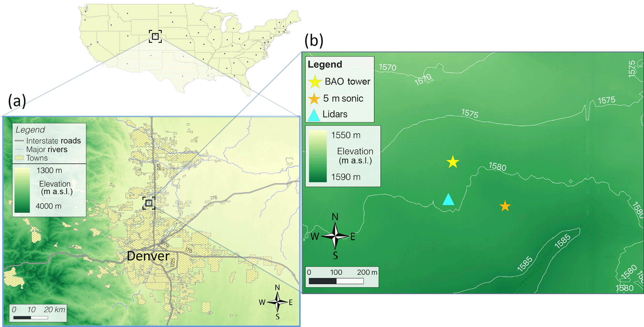
Figure 1Map of the topography of the region where the XPIA field campaign took place. Contours in (b) show elevation in meters above sea level.
2.1 Meteorological tower measurements
During XPIA, the 300 m BAO meteorological tower (Kaimal and Gaynor, 1983) had two 3-D sonic anemometers (Campbell CSAT3) at each of six levels (50, 100, 150, 200, 250, and 300 m a.g.l.), providing measurements with a frequency of 20 Hz (Bianco, 2018). The measurement accuracy was generally less than in the horizontal and in the vertical. At each level, the two sonic anemometers were mounted pointing northwest (334∘) and southeast (154∘). In order to avoid tower wake effects, data from the northwest sonics are discarded when the wind direction was between 111 and 197∘, while wind directions between 299 and 20∘ exclude data recorded by the southeast sonic (McCaffrey et al., 2017b). Data have been tilt-corrected according to the planar fit method described in Wilczak et al. (2001). An additional sonic anemometer was mounted on a 5 m a.g.l. surface flux station located 200 m southwest of the BAO tower over natural arid grassland. The sonic anemometer (Campbell CSAT3A) at this location operated with a frequency of 10 Hz.
We quantify atmospheric stability from the 5 m tower data in terms of the Obukhov length L, defined as
where θv is the virtual potential temperature (K), calculated from the sonic anemometer virtual temperature data Tv and the measured pressure p as with p0=1000 hPa and ; k=0.4 is the von Kármán constant; g=9.81 m s−2 is the gravity acceleration; is the friction velocity (m s−1); and is the kinematic sensible heat flux (W m−2). The turbulent quantities have been separated in average and fluctuating parts using the Reynolds decomposition with an averaging time of 30 min. This timescale is a common choice (Babić et al., 2012; De Franceschi and Zardi, 2003) when studying boundary layer processes since it is generally longer than the turbulence timescales, but also shorter than the mean flow unsteadiness timescales. For atmospheric stability, we classify neutral conditions as and L>500 m, unstable conditions as , and stable conditions as (Muñoz-Esparza et al., 2012). Neutral conditions were rarely detected (less than 5 % of the times) during the period of the campaign.
At the base of the BAO tower, a tipping-bucket rain gauge was used to measure precipitation. We have excluded from our analysis the times within 1 h from precipitation events (∼8 % of the times), as during these cases the measurement accuracy of both sonic anemometers and wind Doppler lidars drops.
2.2 Wind Doppler lidar measurements
Several vertical profiling and scanning wind Doppler lidars were deployed at XPIA. In this study, we focus on three vertical profiling lidars and one scanning lidar mainly used in vertical staring mode. All these instruments were co-located approximately 100 m south of the BAO tower (Fig. 1).
A WINDCUBE version 2 (v2) profiling lidar was deployed by the University of Colorado Boulder from 12 March to 8 June 2015. This lidar samples line-of-sight velocity in four cardinal directions with a nominal 28∘ zenith angle, followed by a fifth vertical beam. Range gates were centered at 40, 50, 60, 80, 100, 120, 140, 150, 160, 180, and 200 m a.g.l. The retrieval of the actual wind speed from this measurement approach assumes horizontal homogeneity across the cone defined by the laser beams during the ∼4 s required to complete a sequence of measurements across the five beams.
Two WINDCUBE version 1 (v1) profiling lidars (Aitken et al., 2012; Rhodes and Lundquist, 2013) were deployed by the University of Colorado Boulder and the National Center for Atmospheric Research from 1 and 4 March 2015 past the end of the experiment. These instruments measure line-of-sight velocity in four cardinal directions (nominal 28∘ zenith angle), with a range resolution of 20 m, from 40 to 220 m a.g.l. The assumption of horizontal homogeneity of the flow in the sampling volume is again necessary to retrieve the actual wind vector. These instruments will be identified in the remainder of the analysis with their serial numbers, 61 and 68.
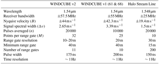
Finally, a Halo Photonics Stream Line Doppler scanning lidar (Pearson et al., 2009) from the U.S. Department of Energy Office of Science Atmospheric Radiation Measurement program was deployed from 6 March to 16 April 2015. This lidar used a range gate resolution of 30 m, with 200 total range gates. However, the maximum range gate with an acceptable number (>30 %) of valid measurements (signal-to-noise ratio, SNR ) was at about 800 m a.g.l. This scanning lidar was mainly used in a vertical staring mode. The scan strategy also included a 40 s plan-position-indicator (PPI) scan at an elevation angle of 60∘ once every 12 min (from which the derivation of the horizontal wind speed is possible), a 10 min tower stare once per hour, and a target sector scan once per day to confirm heading relative to the tower (Newsom et al., 2017). Table 1 includes the main technical characteristics of the three commercial lidar models considered in our analysis.
Table 1Main technical specifications of the lidars at XPIA used in this study.
3.1 Turbulence dissipation from sonic anemometer
Sonic anemometer data can be used to calculate turbulence dissipation rate with two different methods: the inertial subrange energy spectra method and the second-order structure function method. Muñoz-Esparza et al. (2018) analyzed data at XPIA and showed that the second-order structure function method has a lower error in estimating ϵ compared to the inertial subrange energy spectra method, even when shorter overlapping temporal sub-windows are used to obtain a more regular pattern in the spectra. Therefore, we also apply the second-order structure function method to estimate ϵ from sonic anemometer measurements every 30 s, for the 3-month period of XPIA.
According to Kolmogorov's hypothesis, within the inertial subrange the velocity increments, expressed as second-order structure function DU of the horizontal velocity U, can be related to ϵ as
where denotes an ensemble average, and a is the Kolmogorov constant. We assume a=0.52, which is consistent with the range of values present in the literature (Paquin and Pond, 1971; Sreenivasan, 1995). The spatial separations r, which must be within the inertial subrange, can be expressed as temporal velocity increments by invoking Taylor's frozen turbulence hypothesis (Taylor, 1935), so that ϵ can be determined as
where DU(τ) is the second-order structure function of the horizontal velocity U calculated over temporal increments τ. For every ϵ calculation (i.e., every 30 s), the second-order structure function was calculated with a 2 min window for τ, centered at the nominal time at which ϵ is calculated. Then, the fitting to the theoretical model only used the time range between τ=0.1 and τ=2 s. Such a short temporal separation in the data is expected to lie well within the inertial subrange, therefore excluding the undesired contributions from the outer scales which would undermine Kolmogorov's fundamental assumptions. Moreover, despite the reduced size of the chosen time range, the high temporal resolution of the sonic anemometers still guarantees an adequate number of data points to allow a robust estimation of the structure function. Data inspection confirms that the desired theoretical τ2∕3 slope is observed in the chosen range for τ (example shown in the Supplement).
As already mentioned, data were excluded for wind directions waked by the tower. When neither of the two anemometers is affected by tower wakes, ϵ is defined as the average between the two independent values obtained from the two sonics at each height. To quantify the uncertainty in turbulence dissipation rate measurements from the sonic anemometers, we have compared ϵ from the two sonics at each level when neither one was influenced by the tower wake. For each tower boom direction (northwest and southeast), we calculate the median absolute error (MAE) between ϵ from the sonic anemometers mounted on the considered boom direction and the correspondent average value from the two sonics:
In calculating the error, we consider data from all heights, as no significant difference was noticed at different levels. For both the boom directions, we find very similar results, with MAE=19 %, which is reduced to 14 % when a 30 min running mean is applied to the ϵ time series. The distributions of the errors are included in the Supplement. No bias was detected between the retrievals from the sonic anemometers on the two boom directions.
3.2 Dissipation from Doppler lidar
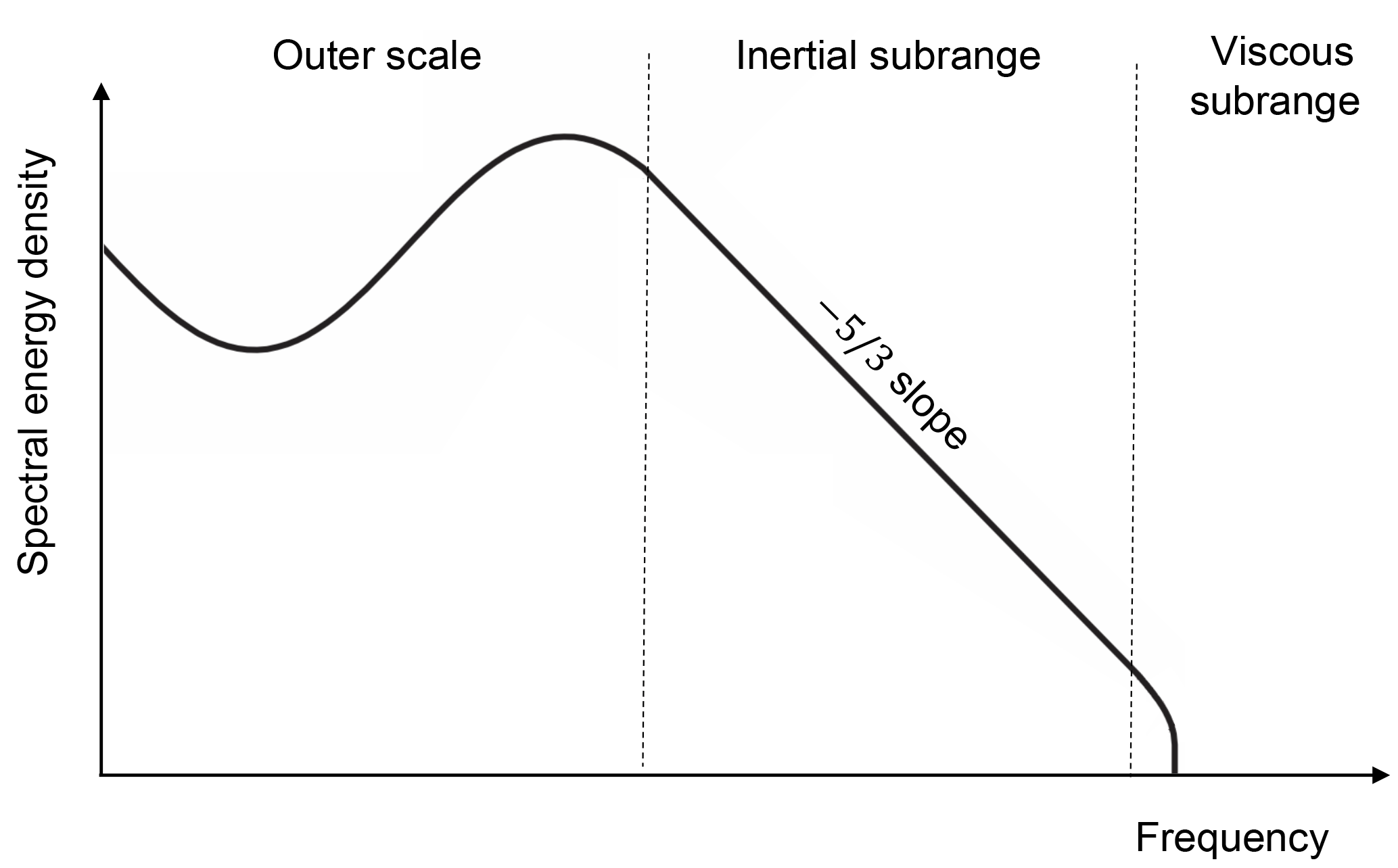
Wind Doppler lidars can provide a great improvement of our understanding of the variability in turbulence dissipation thanks to the ease of their deployment in different locations and the long measurement range allowed by several commercial models. To do so, robust methods to estimate ϵ with lidars are necessary, and their uncertainty has to be assessed. For this purpose, we follow and refine the approach described in O'Connor et al. (2010) to estimate ϵ from vertical profiling lidars or scanning lidars used in vertical staring mode. For homogeneous and isotropic turbulence, within the inertial subrange, the turbulent energy spectrum (Fig. 2) can be expressed according to the Kolmogorov (1941) hypothesis in terms of wave number k as
where a≃0.52 is the one-dimensional Kolmogorov constant. The wave number k can be written in terms of a length scale by invoking Taylor's frozen turbulence hypothesis (Taylor, 1935). By integrating Eq. (5) over the wave number space, starting from the wave number k1 corresponding to a single lidar sample, the variance of the de-trended observed line-of-sight velocity from N samples can be obtained:
and therefore if the length scales are properly chosen (and consistent with how σv is computed) then ϵ can be calculated without the need of systematically computing turbulence energy spectra. In Eq. (6), the length scale L1 for a single sample interval is given by
where U is the horizontal wind speed, t is the dwell time, θ the half-angle divergence of the lidar beam, and z the height above ground level. Since Doppler lidars generally have a very small θ (<0.1 mrad), the second term in Eq. (7) is typically negligible. For N samples, the length scale becomes LN=NUt. For the WINDCUBE lidars, the variance of the observed line-of-sight velocity can be calculated as the average from all the beams. In doing so, we include turbulence contributions from both the horizontal and vertical dimensions, and we make the limiting (Kaimal et al., 1972; Mann, 1994) assumption of isotropic turbulence. For the Halo Stream Line lidar, which operated in a vertical stare mode, is calculated from the vertically pointing beam, and therefore ϵ will strictly include turbulence contributions only in the vertical dimension, thus possibly determining different values compared to what is retrieved from the WINDCUBE lidars. Another difference due to the different scan patterns used by the considered lidars is related to the determination of the horizontal wind speed U. For the WINDCUBE lidars, U can be derived from the line-of-sight velocity measurements from the different beams, with the assumption of horizontal homogeneity of the flow over the probed volume. In the case of the Halo Stream Line, no information about the horizontal wind can be derived from the measurements in the vertical staring mode, which only measures the vertical component of the wind speed. U is then retrieved from a sine-wave fitting from the vertical-azimuth display (VAD) scans that are performed every 12 min. The heights at which the measurements are taken during the tilted VAD scans are not the same as the heights sampled in the vertical staring mode. Therefore, for each considered level in the vertical staring mode, U is determined from a linear interpolation of the wind speed retrieved at the two closest heights during the VAD scans. Considerations about the error introduced by this procedure on the estimation of ϵ will be discussed in Sect. 4.
Lidar measurements are inherently affected by signal noise as well as possible variations in the aerosol fall speeds, which provide additional contributions to the observed variance. By assuming that the contribution of all atmospheric flows to the observed line-of-sight variance within the considered short timescales can be regarded to be of a turbulent nature, the variance in Eq. (6) can be written as the sum of three different terms, which can be considered to be independent of one other (Doviak, 1993):
is the desired net contribution from atmospheric turbulence at the scales that can be measured by the lidar (Brugger et al., 2016), from which the estimation of ϵ can be made. The additional contributions to the variance are due to the instrumental noise () and the variation in the aerosol terminal fall speeds within the measurement volume from different sample intervals (), which however can safely be neglected since the particle fall speed is typically . For a heterodyne Doppler lidar, Pearson et al. (2009) provide the following expression for the noise contribution to the variance, as a function of the SNR:
where Np is the accumulated photon count:
In this expression, n is the number of lidar pulses which are averaged to obtain a profile, and M is the number of points sampled within a single range gate to obtain a velocity estimate. α is the ratio of the lidar photon count to the speckle count (Rye, 1979):
where B is the bandwidth, equivalent to twice the Nyquist velocity, and Δν is the signal spectral width. For the WINDCUBE lidars, is calculated as the average from all the beams. The noise contribution to the observed variance determines an additional area below the turbulence spectrum in its high-frequency region (Frehlich, 2001), which, if not removed, would induce an overestimation of ϵ. Therefore, the turbulence dissipation rate can be estimated as
This method relies on the assumption that both length scales L1 and LN are within the inertial subrange. Therefore, the choice of the number of samples N to use should be carefully addressed since only the turbulence contributions in the inertial subrange should be included in the calculation. We discuss in detail this choice and its relationship with different atmospheric stability conditions and heights in the next section.
Although promising, the method to calculate ϵ from lidar data presented in the last section needs to be carefully analyzed in relation to its fundamental assumptions and its uncertainty, especially given the limited temporal resolution of lidar measurements. In this section we refine the method to derive ϵ from lidar data by discussing, in relationship with different heights and atmospheric conditions, the choice of the number of samples N to use for the calculation of the variance of the de-trended line-of-sight velocity and corresponding length scales. Moreover, we assess the uncertainty of this method by systematically comparing ϵ values from lidar measurements with what is obtained from the sonic anemometers, and we discuss how the estimation error changes with height in the boundary layer.
While the high temporal resolution of sonic anemometers facilitates the identification of sizable samples within the inertial subrange, for lidars, the length of the samples used to estimate the variance of the line-of-sight velocity should be accurately chosen. In fact, the shorter the sampling time, the higher the measurement error in the estimate of the variance of line-of-sight velocity would be, because of both higher measurement uncertainty, which impacts its representativeness (Lenschow et al., 1994), and a higher relative contribution of the instrumental noise. According to the formulation in Lenschow et al. (2000), the measurement error in the turbulence contribution to the observed variance can be estimated as
Therefore it decreases as the number of samples N increases, with the hypothesis that the noise contribution to the variance of each velocity sample used to estimate ϵ is similar to the ensemble mean error.
Conversely, if the sampling time is too long, the variance will incorporate undesired contributions from the large-scale processes, which would cause a severe underestimation of ϵ. Figure 3 shows how the estimated value of ϵ varies with the sample length used in the calculation, for a case using the WINDCUBE v2 data at 100 m a.g.l. As long as the sample length stays within the inertial subrange (up to ∼45 s in the case shown), ϵ stays approximately constant. However, the estimate of ϵ decreases by up to an order of magnitude when the contributions from the outer scales are erroneously included in the calculation, which uses expressions that are valid strictly only within the inertial subrange.
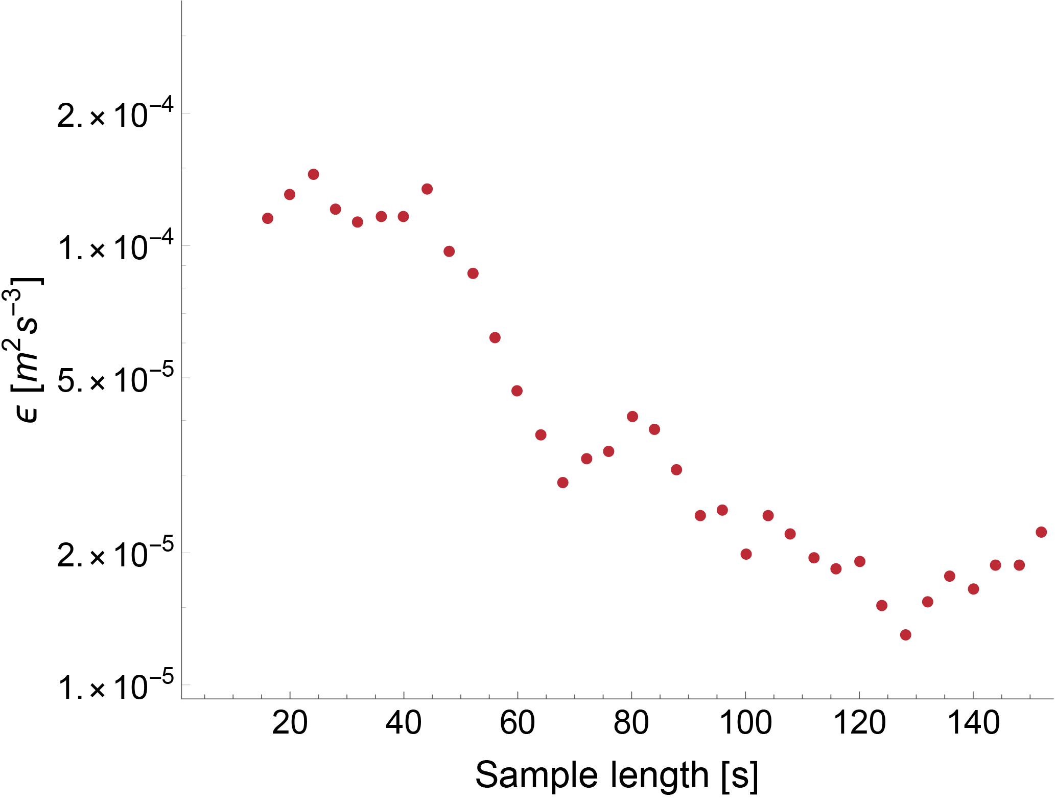
Figure 3Example of the dependence of ϵ on the sample length used in the calculation. Data from the WINDCUBE v2 lidar at 100 m a.g.l., 30 March 2015, 14:20 UTC.
Moreover, since different atmospheric stability conditions are inherently characterized by different turbulence scales (Kaimal et al., 1972), the transition from the inertial subrange to the outer scales occurs for different sample lengths, depending on the atmospheric stability. Figure 4 shows examples of turbulence spectra calculated over 15 min intervals for data measured by the WINDCUBE v2 lidar at 100 m a.g.l. in different stability conditions. For stable conditions (Fig. 4a), the transition from the inertial subrange (which can be identified by comparing the slope of the spectrum with the theoretical value shown by the dashed line) to the outer scales occurs at a higher frequency compared to the unstable case (Fig. 4b). Therefore, the choice of the number of samples N to use in the calculation should change accordingly. As a general rule, we expect shorter timescales to be adequate for stable conditions, when the turbulent eddies in the boundary layer are smaller, while longer scales would be more suitable during unstable conditions, characterized by larger convective eddies that can be fully captured only when using larger scales. Moreover, different altitudes can also impact the extension of the inertial subrange, with a wider development expected at higher heights, as the integral length scale of turbulence increases (Wang et al., 2016).
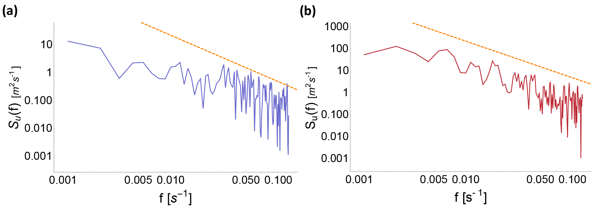
Figure 4Turbulence energy spectrum for a stable case (a – 2 April 2015, 03:00 UTC) and an unstable case (b – 3 April 2015, 22:15 UTC), calculated from 15 min of data measured by the WINDCUBE v2 at 100 m a.g.l. The dashed lines represent the theoretical slope expected in the inertial subrange. To calculate ϵ for these cases, the optimal sample length from comparison with the sonic anemometers corresponds to frequencies greater than 0.04 s−1 for stable conditions and greater than 0.01 s−1 for unstable conditions.
To estimate the appropriate timescales which best balance these competing factors, we calculate ϵ, at each height from each of the considered lidars, using several values for the number of samples N used in the calculation. At the heights at which there is correspondence between lidar and sonic anemometer measurements, we then compare the ϵ values from the lidars with the corresponding ϵ calculated at the meteorological tower. The estimates of ϵ from sonic anemometers and lidars have been calculated at slightly different time stamps, given the unavoidable difference in the nominal measurement time stamps of instruments operating with different temporal resolutions. Given the inherent turbulent nature of ϵ and its remarkable range of variability, the comparison between the time series from sonic anemometers and lidars could be flawed by the effect of the turbulent high-frequency variability in ϵ. Moreover, since this analysis is focused on the assessment of the appropriate timescales for different stability conditions, consistency with the timescale used to calculate turbulent fluxes for the determination of the Obukhov length L is advisable. Therefore, a 30 min running mean is applied to the time series of ϵ from both sonic anemometers and lidars before comparing the estimates from the different instruments.
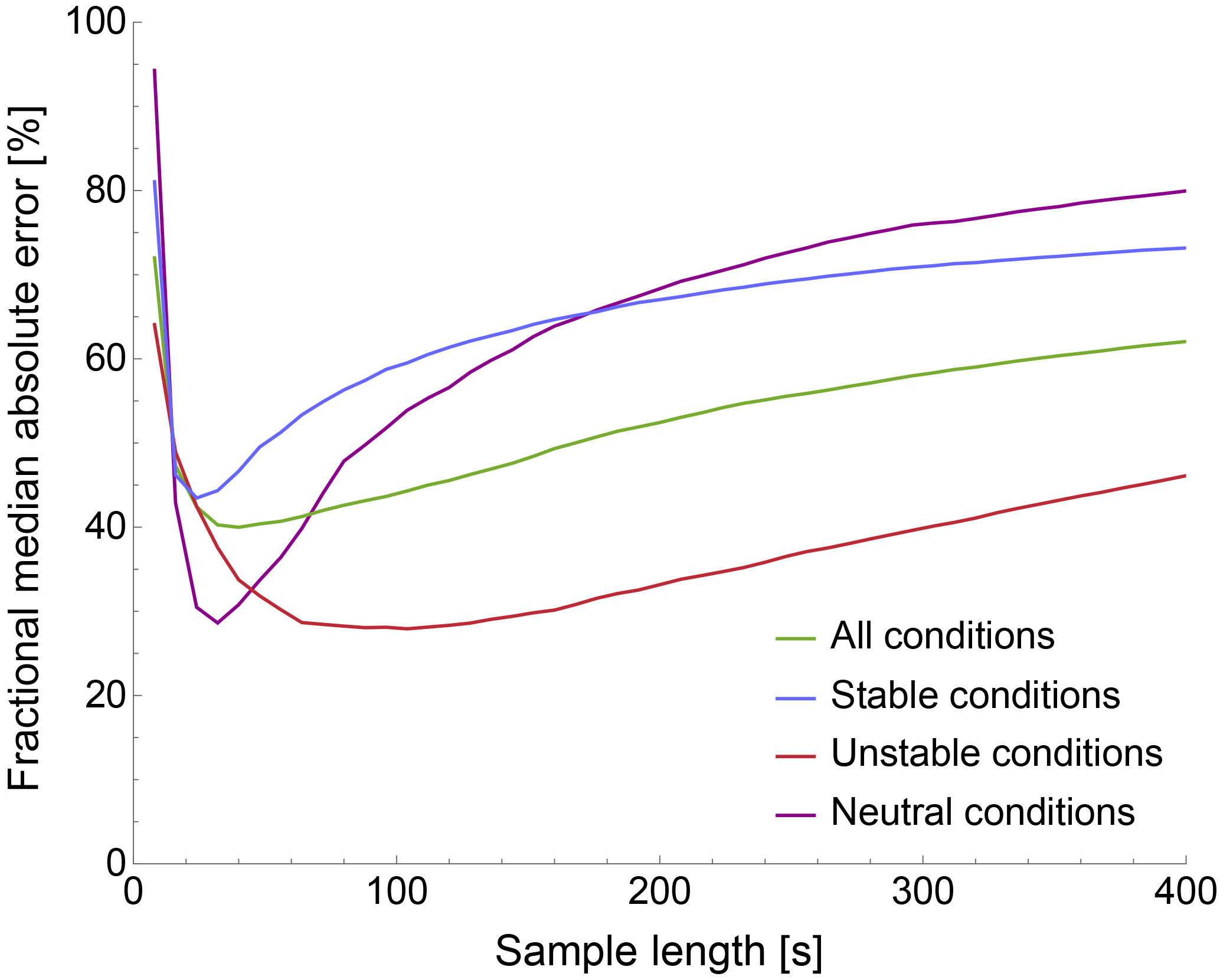
Figure 5Median absolute error between ϵ estimates (smoothed with a 30 min running mean) from sonic anemometer and WINDCUBE v2 lidar data at 100 m a.g.l. during the whole period of the XPIA campaign, as a function of the sample length used to estimate ϵ from lidar data.
To quantify the difference between sonic and lidar estimates of ϵ, we use the median absolute error (MAE), defined as
The result of this comparison is reported in Fig. 5, which shows how the MAE varies with the timescale (calculated as Nt, where t is the dwell time of the considered lidar) used to estimate ϵ for the WINDCUBE v2 lidar, for different atmospheric stability conditions, at 100 m a.g.l.
As the used sample length increases, the average error in ϵ estimated from lidar initially decreases from the high values related to the strong noise contribution at short timescales. Then, a minimum in the error is reached. As the size of the sample further increases, the average error rises again, due to the incorporation of undesired contributions from the outer scales. Moreover, as expected, the minimum error for stable (and neutral) conditions is found to be at shorter timescales than unstable conditions. Also, the minimum error in stable conditions is higher than the minimum error for unstable conditions since the need of using a shorter timescale implies a higher relative contribution of the instrumental noise to the error. The same qualitative pattern is found for all the considered lidars, at all heights. At each height, for each lidar and for each stability classification, we select the timescale that produces the lowest median absolute error compared to the sonic anemometer estimates of ϵ: this can be interpreted as the longest timescale that does not include substantial contributions from the undesired outer scales. Table 2 summarizes the selected timescales for the considered lidars for the different stability conditions (neutral conditions are not shown because they occurred less than 5 % of the time), as well as the average from all the instruments, at 100 m a.g.l.
Table 2Timescales which minimize the median absolute error (MAE) in the comparison between ϵ from sonic anemometers and lidars at 100 m a.g.l. for stable and unstable conditions. Results for neutral conditions are not shown since these were rarely detected during the campaign.
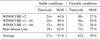
As expected, the larger eddies which characterize unstable conditions determine the need for a longer timescale to capture the influence of all the scales included in the inertial subrange, while for stable conditions a shorter timescale is more appropriate. The median error is higher during stable conditions (average: MAE =51 %) compared to unstable conditions (average: MAE =29 %), as expected and as observed in other studies (Smalikho and Banakh, 2017).
Looking at the variability in the results with height, we find that the optimal timescales increase with height. At those heights <300 m a.g.l. at which lidar measurements do not match the level of any sonic anemometer on the meteorological tower, the adopted timescales are chosen as averages among the scales at the closest levels covered by sonics. For the Halo Stream Line lidar, whose measurements are considered up to 800 m a.g.l. in this study, we determine the appropriate sample sizes by linearly extrapolating aloft, for each stability condition, the sequence of the chosen scales at the lower levels, where a comparison with the meteorological tower data is possible. The linear trend matches the observed results up to 300 m well, with R2>0.9 for all stability conditions (plot shown in the Supplement). Moreover, the rationality of the chosen scales at high altitudes has been confirmed after inspecting the extension of the inertial subrange in turbulence spectra from the Halo Stream Line lidar data (figure not shown).
Once the appropriate timescales have been identified at each height, considerations about how the error in lidar estimates of ϵ varies with height can be made. Figure 6 shows how the MAE between lidar and sonic estimates of ϵ changes with height, for all the levels at which sonic anemometers were mounted on the BAO tower. When a match between the height of lidar measurements and the level of the sonics was not present, the median error shown in the plot has been estimated as the average between the errors at the two closest lidar range gates. For the WINDCUBE v1-68, data at 50 m a.g.l. are not available because of measurement contamination due to hard strikes with the guy wires of the meteorological tower. The same issue invalidates measurements at 140 m a.g.l. from the WINDCUBE v1-61, so the comparison with the sonic anemometer at 150 m a.g.l. has been performed using only this lidar's data measured at 160 m a.g.l. For the Halo Stream Line, measurements below 105 m a.g.l. show a high percentage of low SNR data and are therefore not reported.
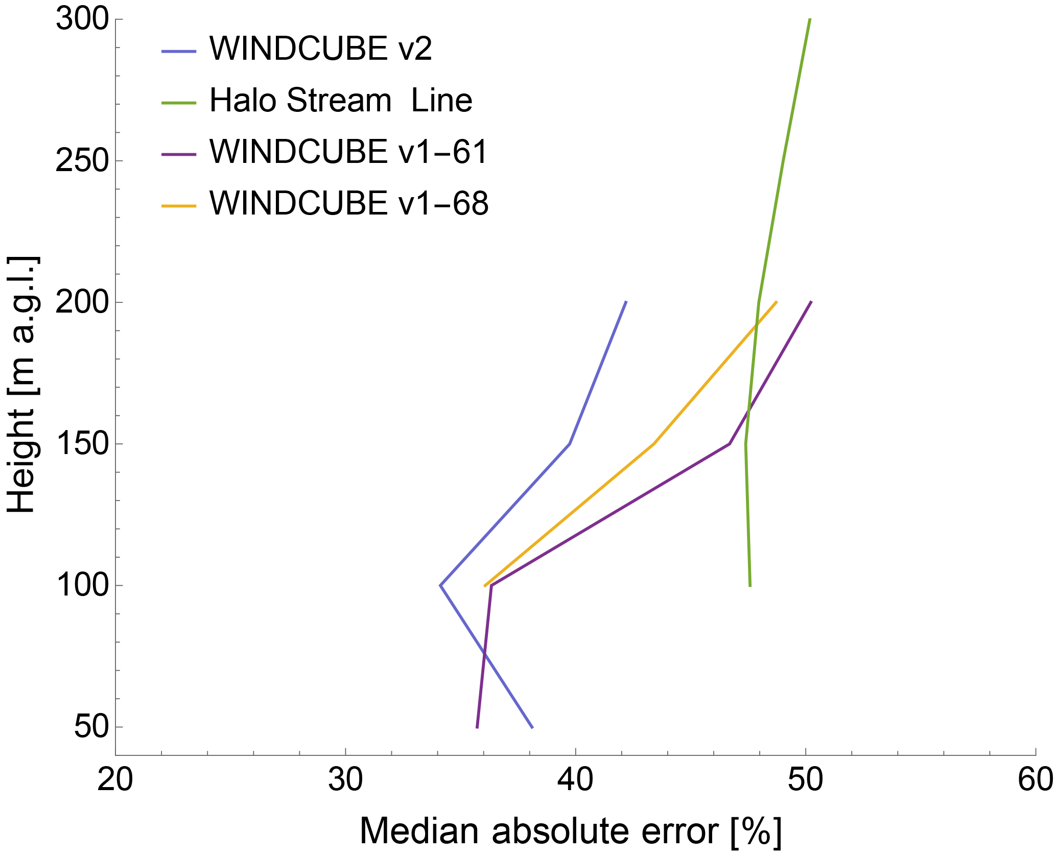
Figure 6Variability in the minimum median absolute error (calculated for the optimized number of samples at each height for each atmospheric stability condition) between lidar and sonic anemometer estimates of ϵ (smoothed with a 30 min running mean) with height, for the four considered lidars.
For the WINDCUBE lidars, the MAE slightly increases with height, likely because of the severe reduction of the number of acceptable measurements at higher levels, and it always stays below 50 %. For the Halo Stream Line lidar, the median error stays almost constant in the considered portion of the boundary layer. It is reasonable to explain the higher error () of the Halo Stream Line compared to the WINDCUBE lidars at 100 m a.g.l. as a consequence of the differences in the spatial dimensions that are sampled by the two lidars. While the lidar beams of the WINDCUBE are tilted, and they therefore include turbulence contributions in the horizontal dimension (which is the only contribution considered in the determination of ϵ from the sonic anemometers), ϵ from the Halo Stream Line is only retrieved using information from the vertically pointing beams. Moreover, the necessary approximations adopted in the determination of the horizontal velocity U for the Halo Stream Line lidar, as explained in Sect. 3.2, likely contributes an additional error for this lidar. However, the magnitude of this additional error due to the reduced frequency in determining U for the Halo Stream Line is comparable to the additional uncertainty related to the drop in instrumental performance that the WINDCUBE shows at higher levels. Therefore, the estimates of ϵ from the Halo Stream Line can be considered physically robust in the lowest few hundred meters of the boundary layer.
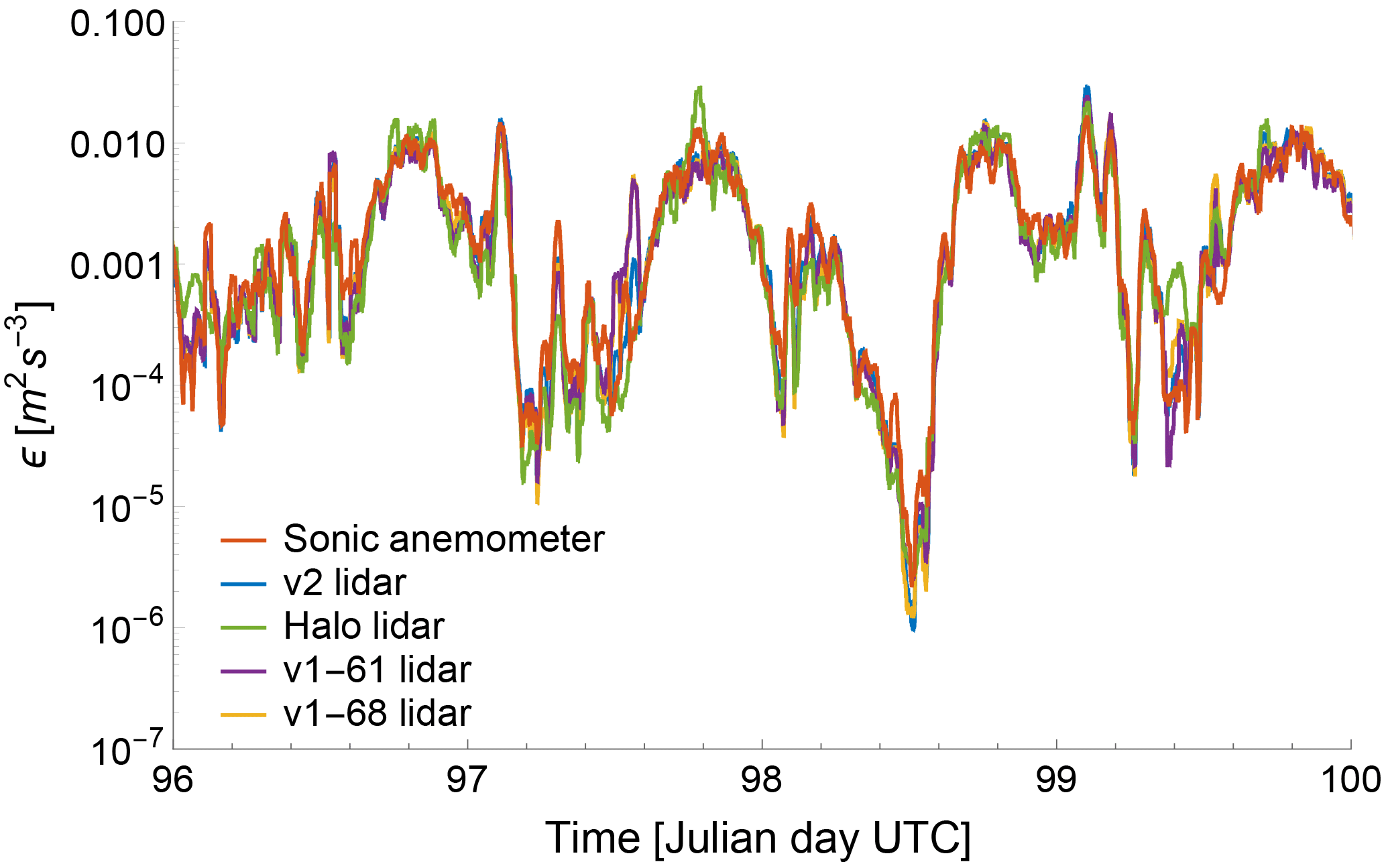
Figure 7Time series from 6 April 00:00 UTC to 10 April 2015 00:00 UTC comparing ϵ from sonic anemometers and all the considered lidars at 100 m a.g.l. Data have been smoothed with a 30 min running mean.
Possible sources for the discrepancy found between ϵ from sonic anemometers and lidars might arise from the different temporal resolution and sampling volumes of the various instruments, as well as the 100 m spatial separation between the lidar site and the BAO meteorological tower. In any case, given the wide range of variability in ϵ, which can span ∼6 orders of magnitude during its typical diurnal cycle (Sect. 5), and the inherent uncertainty in the sonic anemometers' retrievals of ϵ (Sect. 3.1), the obtained magnitudes of the error prove that the refined method to retrieve ϵ from lidar measurements gives robust estimates of turbulence dissipation rate. The accommodation for different stability conditions in the choice of the timescales used in the method considerably reduces, especially for stable conditions, the magnitude of the errors (obtained through propagation of errors) found in the original study (O'Connor et al., 2010). To visualize the good agreement between sonic anemometer and lidar estimates of ϵ, Fig. 7 shows the time series for a portion of the XPIA campaign, with values from all the considered instruments at 100 m a.g.l. A clear diurnal pattern is revealed, with higher values of turbulence dissipation during the day, and differences of several orders of magnitude between daytime and nighttime values of ϵ. These results will be explored in more detail in Sect. 5. A systematic comparison between ϵ estimates from sonic anemometers and the WINDCUBE v2 lidar at 100 m a.g.l. is shown by the density histograms in Fig. 8, for the whole period of the XPIA campaign, for different stability conditions and smoothing. The coefficient of determinations R2 is also reported in the plots.
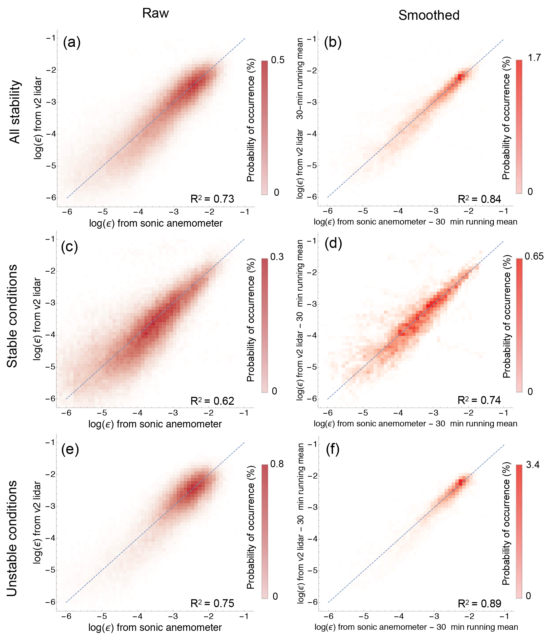
Figure 8Correlation between ϵ values from sonic anemometer and WINDCUBE v2 lidar at 100 m a.g.l. for the whole period of the XPIA campaign, using the selected timescales for the estimation of ϵ from lidar data. The color scales represent the probability of occurrence as a percentage, and the dark dashed lines show perfect correlation. (a) All stability conditions, raw data (MAE = 62 %); (b) all stability conditions, 30 min running mean applied (MAE = 34 %); (c) stable conditions, raw data (MAE = 67 %); (d) stable conditions, 30 min running mean applied (MAE = 44 %); (e) unstable conditions, raw data (MAE = 58 %); (f) unstable conditions, 30 min running mean applied (MAE = 27 %).
The good agreement between data from sonic anemometer and lidars is confirmed, with unstable conditions showing a better performance (R2=0.89 for the smoothed time series) compared to stable conditions (R2=0.74). Moreover, the plots show the effect of the choice of applying the 30 min running mean before comparing ϵ values from the different instruments. In Fig. 8, the panels on the left compare ϵ without any temporal filter (one value every ∼4 s), while the panels on the right show the comparison among time series after the 30 min running mean has been applied. The application of the 30 min running mean to the ϵ time series increases the correlation among the different time series. In any case, even for the raw time series, the values of the coefficient of determination are always greater than 0.6.
Determination of the optimal timescales to retrieve ϵ from lidars in absence of co-located sonic anemometers
The availability of multiple sonic anemometers co-located with the lidars at XPIA has allowed for a direct comparison among ϵ estimates from different instruments to determine the optimal length scales, in different stability conditions, to use when retrieving ϵ from Doppler lidar measurements. This approach does not require the direct calculation of spectra from the line-of-sight velocity measured by the lidars, and therefore it represents a time-efficient technique. However, the proposed method is only viable when sonic anemometers are deployed in the near vicinity of a lidar, and when measures of atmospheric stability are available.
When a comparison with sonic anemometer data is not possible, the appropriate timescale to use in the lidar retrieval of ϵ can be determined by finding the maximum wavelength within the inertial subrange in the velocity spectra from the lidar measurements. To do so, spectral models can be fit to the observed spectra. Several models have been proposed for turbulence spectra in different stability conditions (Kaimal et al., 1972; Olesen et al., 1984; Panofsky, 1978). We test the spectral model proposed by Kristensen et al. (1989), which proposes expressions for the cases of both an isotropic and an anisotropic horizontally homogeneous flow, without assumptions on the stability condition. To validate our results and test this alternative approach to derive ϵ from lidar measurements, we use data from the Halo Stream Line lidar to estimate the maximum wavelength λz within the inertial subrange. Since the Halo mainly operated in a vertical stare mode during XPIA, we consider the following expression for the turbulence spectrum of the vertical component of the wind speed, assuming an anisotropic horizontally homogeneous flow:
where k is the wave number, σz is the standard deviation of the vertical component of the wind speed used to compute the spectrum, lz is the integral scale of the vertical velocity along the horizontal flow trajectory, and the parameter μ controls the curvature of the spectrum. We use μ=1.5, which provides a good match with our experimental spectra, as also found in previous studies (Lothon et al., 2009; Tonttila et al., 2015). The parameter a can be expressed as a function of μ as
We calculate spectra using 10 min consecutive data, and we fit the spectral model to the experimental data, leaving out frequencies greater than 0.2 Hz, which are affected by instrumental noise (Frehlich, 2001), not modeled here. An example of a measured spectrum and the fit resulting from the model are shown in Fig. 9.

Figure 9Example of power spectral density of the vertical component of the wind speed as measured by the Halo Stream Line lidar on 11 March 2015 18:05 UTC. The red line represents the fit according to the spectral model from Eq. (15); the orange dotted line shows the theoretical slope.
The transition wavelength λz between the inertial subrange and the outer scales can be expressed as a function of the integral scale lz and the parameter μ:
Following the approach in Tonttila et al. (2015), we estimate the timescale corresponding to this transition wavelength by dividing λz by the collocated wind speed derived from the closest PPI scan performed by the Halo Stream Line lidar.
To compare the results from this approach with what we obtain from the comparison with dissipation rates from the sonic anemometer data, we apply this technique to the data from the Halo Stream Line for the whole period of XPIA and calculate the average timescales for different stability conditions at 100 m a.g.l. We obtain an average timescale of 32 s in stable conditions and 73 s in unstable conditions. Both these values compare well with what is found with the more time-efficient comparison with the sonic anemometer retrievals (values in Table 2), thus confirming that the use of spectral models can be considered a valid alternative for the determination of the optimal sample lengths to retrieve ϵ from lidar data.
The use of spectral models to determine the appropriate sample size to use when retrieving ϵ from lidars can also be applied when information about atmospheric stability is not available or accurate. In these cases, instead of calculating an average optimal sample size for each stability condition, an appropriate timescale can be determined at each time ϵ from lidar measurements, from a single spectrum. We compare ϵ values from the sonic anemometers and from the Halo Stream Line lidar, with the optimal timescales obtained from both the proposed approaches (comparison with the sonic anemometer data and analysis of instantaneous spectra) in Fig. 10, for the same time period shown in Fig. 7.
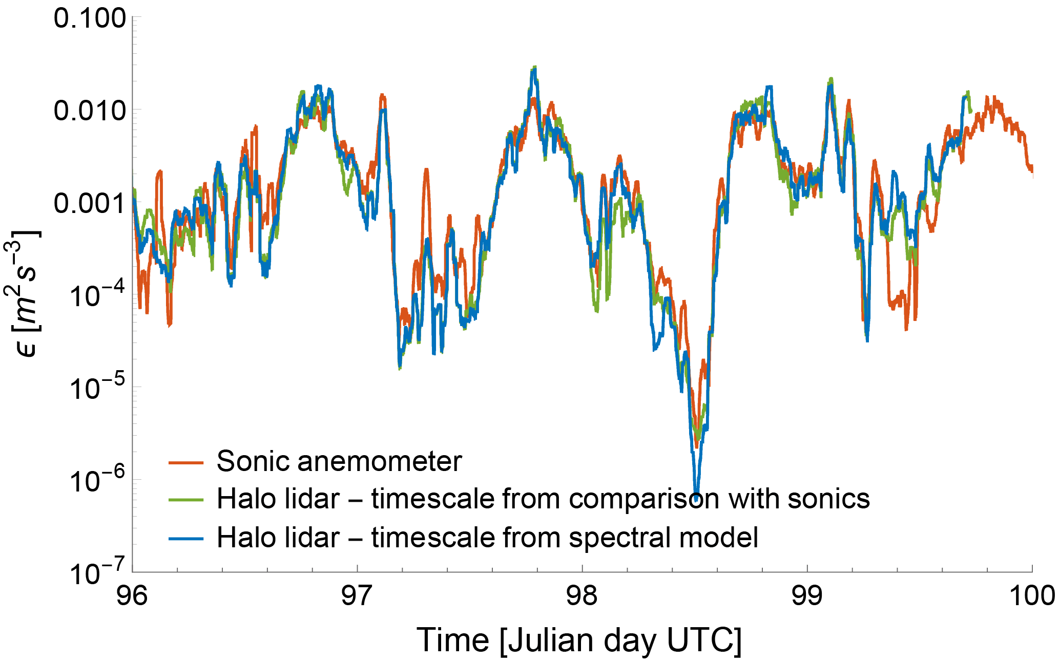
Figure 10Time series from 6 April 00:00 UTC to 10 April 2015 00:00 UTC comparing ϵ from sonic anemometers and the Halo Stream Line lidars at 100 m a.g.l., where the timescales for the lidars have been determined with both the proposed approaches (comparison with ϵ from sonic anemometers and fit with spectral models). Data have been smoothed with a 30 min running mean.
The use of spectral models to determine the extension of the inertial subrange in the lidar spectra produces valid estimates of ϵ: for this case we obtain a MAE =40 % and a correlation coefficient R2=0.78.
Once the capability of the method to provide accurate estimates of ϵ from lidar data has been tested, the variability in turbulence in the boundary layer can be assessed using data from the various instruments deployed at XPIA.
The time series of ϵ shown in the previous section revealed that, during the course of the day, ϵ changes by several orders of magnitude. To better explore this diurnal variability, Fig. 11 shows the daily climatology of turbulence dissipation rate, calculated as the median of the data from the sonic anemometer, WINDCUBE v2 lidar, and Halo Stream Line lidar. Plots for the two WINDCUBE v1 lidars are shown in the Supplement and are similar to the results from the WINDCUBE v2.
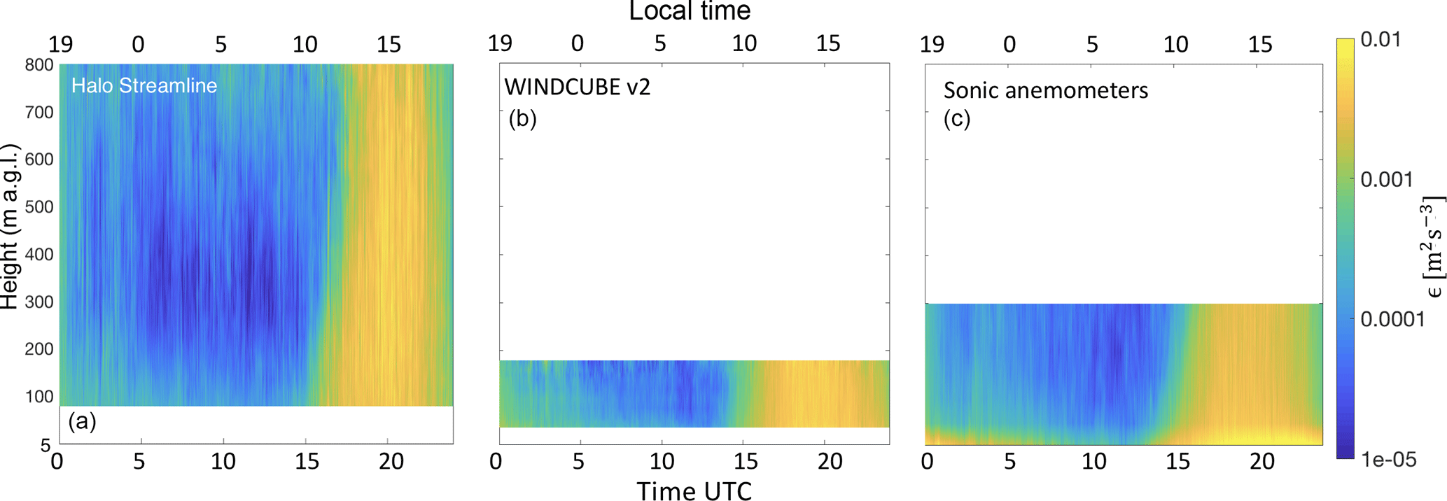
Figure 11Daily climatology of turbulence dissipation rate derived from raw values from the Halo Stream Line (a), the WINDCUBE v2 lidar (b), and sonic anemometers (c). Results from the two WINDCUBE v1 lidars are included in the Supplement.
A general good agreement between the climatology from sonic anemometers and lidars can be observed. A definite diurnal pattern is evident from each panel. As expected, the mainly quiescent conditions at night determine low values of turbulence dissipation rate (), while daytime convection increases the median turbulence dissipation in the boundary layer by several orders of magnitude (). During nighttime, however, the median values of ϵ show more variability than during daytime conditions, as traces of intermittent bursts of ϵ can be detected in the climatology. We will investigate these changes in ϵ in more detail, by relating the variability in ϵ with wind speed, especially in the case of nocturnal low-level jets.
Also, the study of the climatology of ϵ can give insights into how ϵ changes with height. The analysis of the climatology from the sonic anemometers (right panel in Fig. 11), which allow measurements of ϵ at 5 m a.g.l., shows how ϵ is higher close to the surface throughout the day, while above 50 m a.g.l. the change of ϵ with height is less noticeable. A similar result can be found from lidars, which provide ϵ measurements starting at 40 m a.g.l. for the WINDCUBE v2 and 75 m a.g.l. for the Halo Stream Line, with reduced variability in ϵ with height in the majority of the sampled height range. The slight increase in ϵ above ∼600 m a.g.l. at night for the Halo Stream Line lidar (left panel in Fig. 11) can be explained as due to more random errors in the line-of-sight velocity measured by the lidar at high altitudes but also as an effect of the higher frequency of good-quality measurements at higher levels during high wind speed events, which determine higher turbulence, as will be shown later in this section. A systematic analysis of how turbulence dissipation rate varies with height is shown in Fig. 12. For each instrument, the percentage difference in ϵ is shown, and it is calculated by taking as reference value the ϵ value closest in time to the sonic anemometer at 5 m a.g.l., so that a common reference level is identified for all the instruments. The continuous line in the plot shows the median value at each height, while the shaded band represents the first and third quartiles of the data distribution.
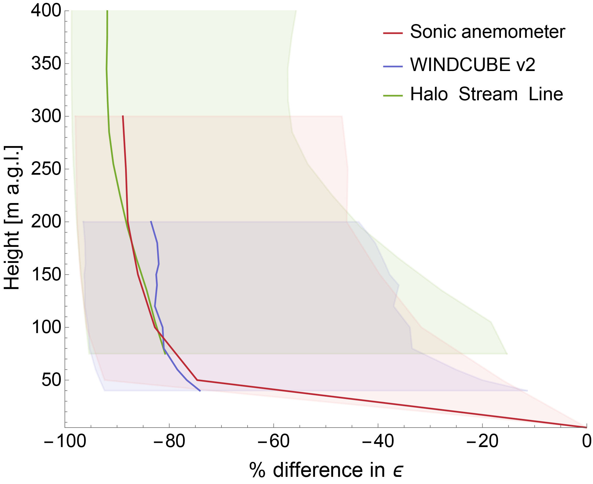
Figure 12Turbulence dissipation rate (raw values) as a function of height for different instruments. The variability with height is expressed as percentage change assuming a reference level of 5 m a.g.l. The continuous line in the plot represents the median value for different instruments, while the shaded area creates a band corresponding to the first and third quartiles of the values.
The plot confirms that turbulence dissipation rate shows most of its variability with height close to the surface, as also found by Balsley et al. (2006). A 75 % decrease in the median ϵ value is observed moving from 5 to 50 m a.g.l. for the sonic anemometer data. We expect this large reduction in ϵ to be due to a rapid decrease in shear production with height close to the surface, as it has been shown (Nilsson et al., 2016) that shear production has a strong connection with dissipation close to the surface. An additional increase in height determines a lower rate of average reduction of ϵ with height, with the median ϵ values for the sonics experiencing an additional 15 % reduction (compared to the reference 5 m a.g.l. level) between 50 and 300 m a.g.l. Variations in comparable magnitude are also found for the lidar data, for both the WINDCUBE v2 and the Halo Stream Line. In any case, the spread around the median value is quite extensive at all the considered heights for all the instruments.
The effect of different atmospheric stability conditions on turbulence dissipation can be investigated in more detail by relating ϵ with the correspondent Obukhov length (L) values, which are used here as a measurement of stability. Figure 13 shows the relationship between turbulence dissipation rate and the absolute value of L, for the sonic anemometers, the WINDCUBE v2, and the Halo Stream Line, at 100 m a.g.l. For each instrument, we sort ϵ based on L. Then, we sub-divide the ϵ data corresponding to equally spaced (in the logarithmic space) L bins. The median ϵ in each group is shown by the continuous line in the plot. The shaded area shows the range between the first and third quartiles. Results from raw ϵ data (i.e., without the application of the 30 min running mean) are shown in the plot. However, no substantial differences arise from the use of the smoothed time series. The Supplement includes the plot for the WINDCUBE v1 lidars, which provides results very similar to what is shown here.
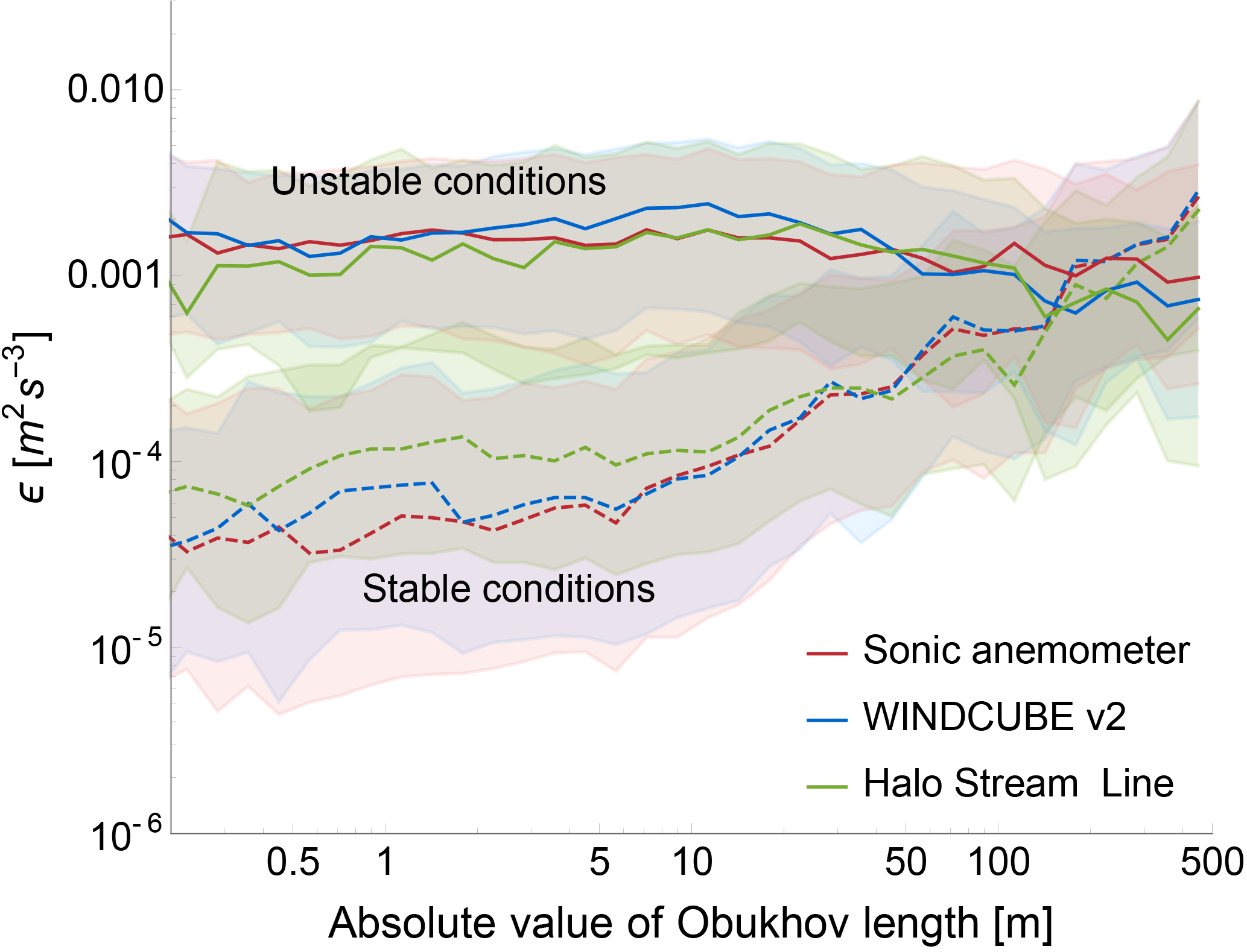
Figure 13Turbulence dissipation rate (raw values at 100 m a.g.l.) as a function of the absolute value of the Obukhov length L. The thick lines in the plot represent the median value for the different instruments, while the shaded area creates a band corresponding to the first and third quartiles of the distributions. Continuous (dashed) lines for unstable (stable) conditions. Results from the two WINDCUBE v1 lidars are included in the Supplement.
Different stability conditions systematically change the magnitude of turbulence dissipation rate, with median ϵ values during strong stable conditions (L>0 m) generally 2 orders of magnitude lower than what is found for strongly unstable conditions (L<0 m). Moreover, as the atmospheric stability conditions become less strong, with an increase in the absolute value of L, the median ϵ values tend to converge to a common value, with ϵ in stable conditions recording a higher increase compared to the change in ϵ for different values of L in unstable conditions. Results from neutral conditions are not shown as they rarely occurred at the site during the field campaign.
Different wind speed regimes can also have a strong impact on the development and subsequent dissipation of turbulence. Figure 14 relates turbulence dissipation rate with 2 min average wind speed, for different stability conditions, at 100 m a.g.l. (results for WINDCUBE v1 lidars are included in the Supplement as very similar to what is found for version 2). The same sampling technique described for Fig. 13 to define median ϵ values, shown by the continuous line, has been applied in this case. Data from the Halo Stream Line are not included here since the reduced temporal availability of horizontal wind speed measurements (once every 12 min) does not guarantee a precise estimation of the variability in ϵ with wind speed for this instrument.
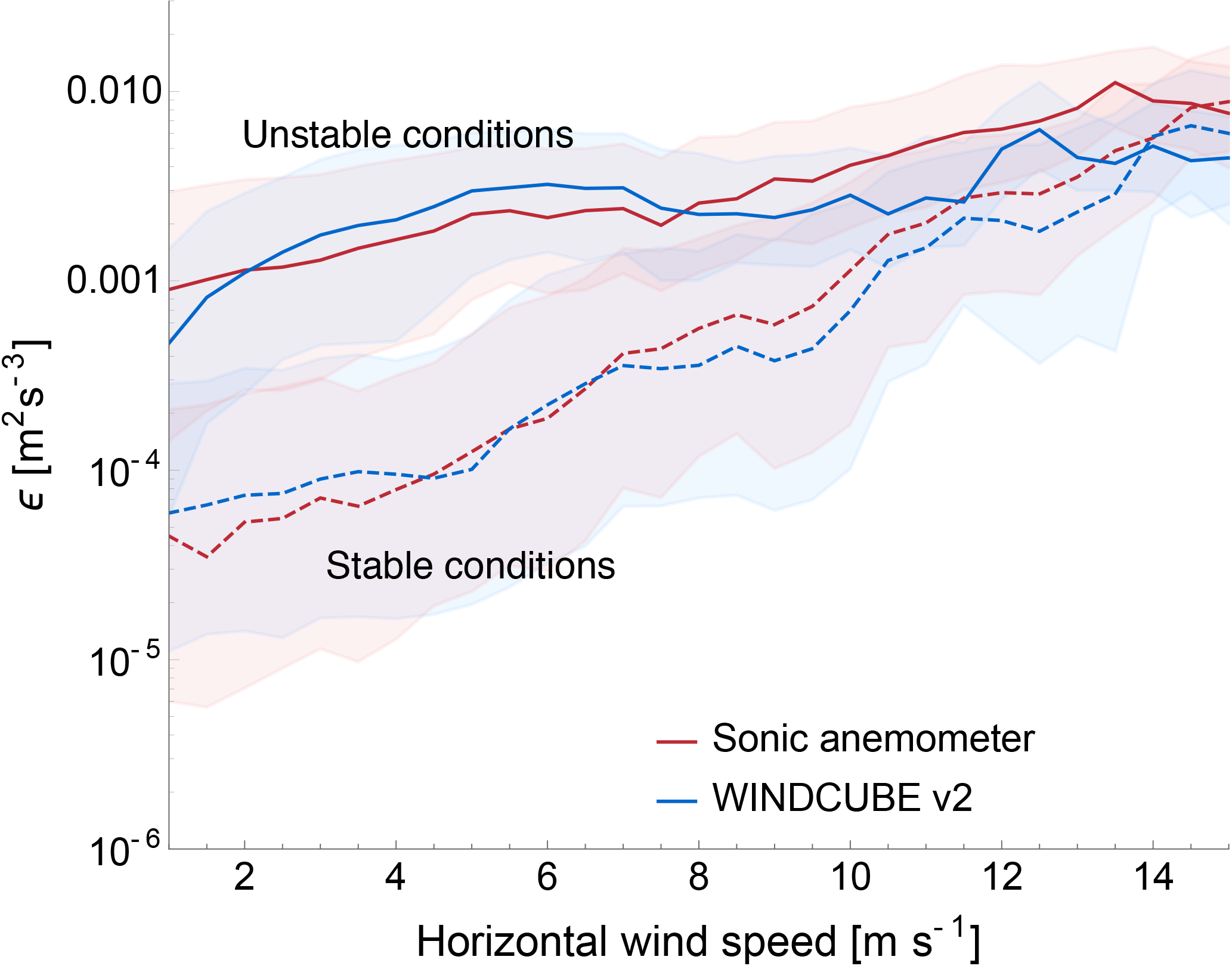
Figure 14Turbulence dissipation rate (raw values) as a function of the 2 min average wind speed, as measured at 100 m a.g.l. The thick lines in the plot represent the median value for the different instruments, while the shaded area creates a band corresponding to the first and third quartiles of the distributions. Continuous (dashed) lines for unstable (stable) conditions. Results from the two WINDCUBE v1 lidars are included in the Supplement.
For both the sonic anemometer and the WINDCUBE v2 lidar data, a strong dependence of ϵ on wind speed can be observed. As wind speed increases, more turbulence is generated – and therefore dissipated – in the boundary layer. The median ϵ increases by 1–2 orders of magnitude as wind speed intensifies from 1 to 15 m s−1. This positively correlated trend is found for both stable and unstable conditions, with ϵ in stable conditions being more subject to variations with wind speed compared to ϵ in unstable conditions. Also, the difference in ϵ during distinct stability conditions becomes less pronounced as the wind speed increases. Therefore, high wind speeds seem to determine strong turbulence – and turbulence dissipation – without any significant dependence on the stability condition.
Turbulence dissipation rate during nocturnal low-level jet events
The accurate numerical representation of nocturnal low-level jets has a crucial importance. In fact, this sudden increase in wind speed aloft at night has been shown to have a primary effect on turbulent transport (Prabha et al., 2007), clear-air turbulence (Banta et al., 2002), storm formation (Curtis and Panofsky, 1958), forest fire propagation (Barad, 1961), and wind energy resources (Vanderwende et al., 2015). In all these cases, turbulence represents an essential driving mechanism, and therefore turbulence dissipation needs to be represented with particular attention. During XPIA, nocturnal low-level jets have been observed several times (Lundquist et al., 2017). As a case study, Fig. 15 shows how wind speed, wind direction, and turbulence dissipation rate varied during the night between 6 and 7 April 2015, as measured by the Halo Stream Line lidar. The analysis of the weather maps for this period reveals no frontal passage during the low-level jet event, while a quasi-stationary front likely occurred at the end of the event (∼ 23:00 LT), as also confirmed by the shift in wind direction during this period, as shown in Fig. 15b. No precipitation was recorded and the analysis of ceilometer data reveals clear sky.
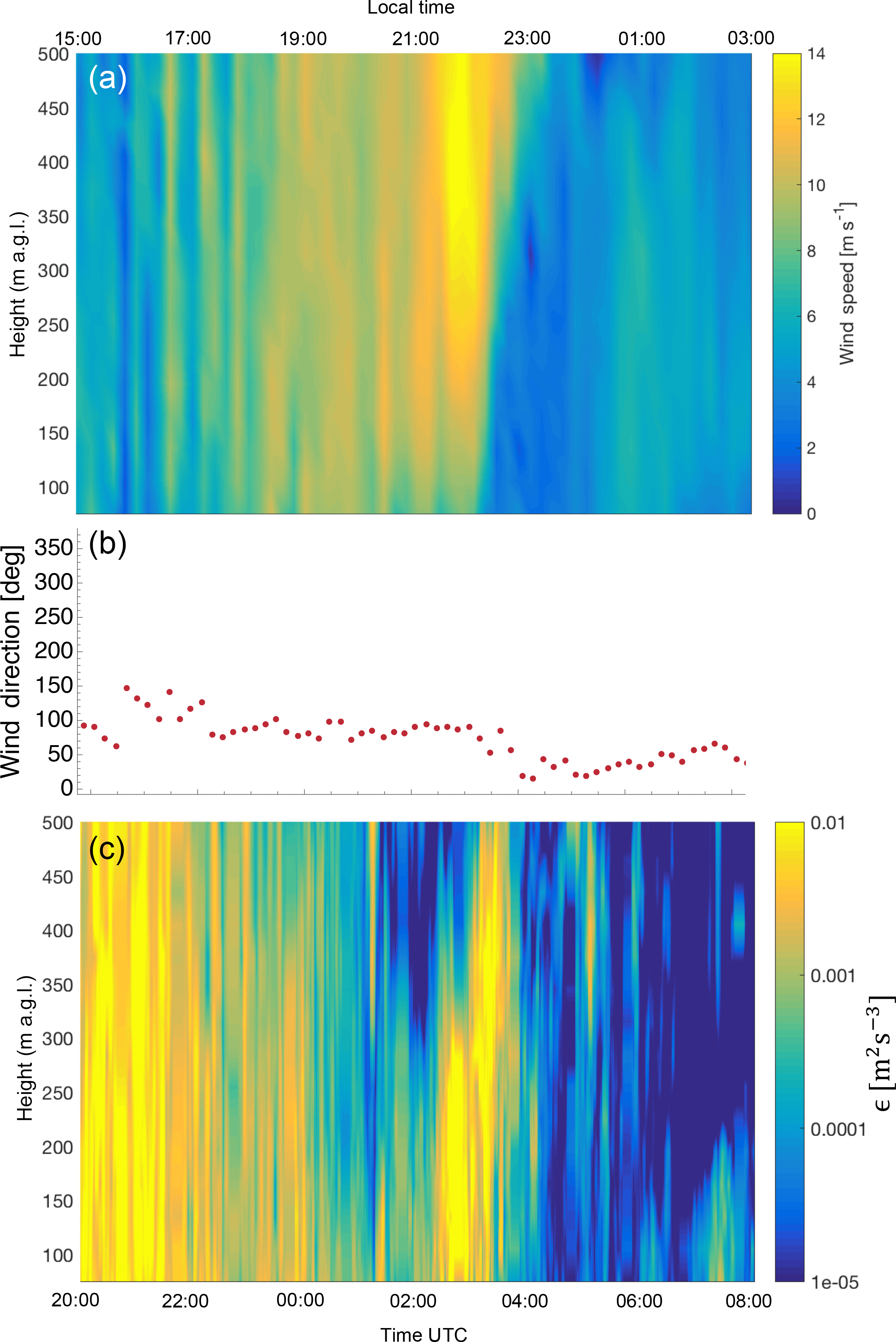
Figure 15Nocturnal low-level jet case study. (a) Variability in wind speed from 20:00 UTC, 6 April 2015, to 08:00 UTC, 7 April 2015, as measured by the Halo Stream Line lidar. (b) Wind direction at 116 m a.g.l., during the same period of time. (c) Corresponding variability in turbulence dissipation rate ϵ as derived from the Halo Stream Line measurements.
A considerable increase in wind speed (up to 14 m s−1, Fig. 15a) can be observed between 21:00 and 23:00 LT. In correspondence to this jet, turbulence dissipation rate (Fig. 15c) increases by at least an order of magnitude throughout the considered vertical portion of the boundary layer, as a consequence of an increase in wind speed variance, as observed in previous studies (Banta et al., 2006). ϵ reaches values of , which are comparable to what is observed during daytime convection, as can be seen between 15:00 and 17:00 LT in the presented case. This abrupt increase in ϵ, which interrupts the normal decrease in ϵ due to the transition from daytime convection to nocturnal quiescence, can also clearly be detected in the time series shown in Fig. 7. After the end of the low-level jet event, in combination with the development of the quasi-stationary front, the return to more quiescent conditions, typical of the nighttime stable boundary layer, causes a considerable reduction of turbulence dissipation rate. Therefore, the turbulence generated by the strong wind acceleration during nocturnal low-level jets can deeply modify the daytime climatology of ϵ, determining the temporary increases which have been detected in the analysis of the climatology in Fig. 11.
Turbulence parametrizations currently used in numerical models have been proven (Yang et al., 2017) to have considerable limitations which undermine the quality of representations of processes in the atmospheric boundary layer. A crucial parameter in this regard is the turbulence dissipation rate (ϵ). Currently, most mesoscale planetary boundary layer models make the assumption of local equilibrium between production and dissipation of turbulence. In this study, we have demonstrated the value of observations from both in situ and remote-sensing instruments in providing insights on the variability in turbulence dissipation rate, and we have assessed how ϵ changes with atmospheric stability, wind speed, and height in the boundary layer.
We have refined an approach to use wind Doppler lidars to quantify ϵ. Our analysis provides recommendations about the choice of the length of sample of lidar measurements to calculate ϵ. In fact, the properties of the turbulence energy spectra for different atmospheric stability conditions have to be taken into account to balance the competing needs of keeping the sampled scales within the inertial subrange, while minimizing the impact of the instrumental noise. We found that longer timescales are appropriate for unstable conditions, while shorter scales should be used in stable cases. Also, the choice of the appropriate sample size should consider the variability of turbulence spectra with height, with longer scales more suitable aloft. The choice of the appropriate timescales can be made by either comparing lidar estimates of ϵ with sonic anemometer data in different stability conditions and heights or by inspecting the properties of the turbulence spectra from lidar measurements with the use of spectral models.
We have tested our methodology by calculating ϵ from four wind Doppler lidars deployed during the XPIA field campaign at the BAO in spring 2015. We have systematically compared the lidar estimates of ϵ with reference data from sonic anemometer measurements to determine the appropriate timescales to use in the calculation. Considering that ϵ spans several orders of magnitude throughout its diurnal cycle, our results reveal good agreement between lidar and sonic anemometer estimates of ϵ, with median differences lower than 30 % in unstable conditions and lower than 50 % in stable conditions.
This analysis reveals that different stability conditions have a considerable impact on determining the magnitude of ϵ. This dual pattern determines the diurnal climatology of ϵ, with lower values during nighttime quiescent conditions and increased turbulence during the daytime convection, as would reasonably be expected. However, the general pattern of the climatology of ϵ strongly varies based on turbulence generation and dissipation due to the magnitude of wind speed. We have found that higher wind speeds cause increased turbulence dissipation, with the gap between ϵ values in stable and unstable conditions becoming less pronounced as the wind speed increases. Therefore, important boundary layer processes such as nocturnal low-level jets can induce a substantial increase in ϵ at night, with values which can reach those of daytime convective turbulence. Finally, we have shown how most of the variability in ϵ occurs in the lowest part of the boundary layer, with a 75 % reduction from 5 to 50 m a.g.l.
The results from this dataset represent significant progress towards the full understanding of how turbulence dissipation varies in the boundary layer. The promising results of the method we propose to retrieve ϵ from lidar measurements make a considerable number of data, measured in the recent years with vertical-profiling lidars, now potentially available to create an extensive database of turbulence dissipation rate for different atmospheric and topographic conditions. Wide deployments of lidars can in fact provide measurements in several different locations and at heights which are not accessible to traditional tower measurements. Future work should include testing the capability of lidars to measure turbulence dissipation rate in complex terrain, with potential case studies including mountain wave phenomena and diurnal circulations, as well as during other specific boundary layer processes, such as horizontal rolls (Brooks and Rogers, 1997). A complete assessment of the variability in ϵ in different terrains would in fact improve our understanding of the main drivers which determine the development and dissipation of turbulence in various conditions. Once the variability in ϵ will be fully captured using different datasets, the implementation of improvements to the turbulence parametrizations used in numerical models will be possible.
The data of the sonic anemometers (Bianco, 2018) and wind Doppler lidars at the XPIA field campaign are publicly available at https://a2e.energy.gov/data (last access: 18 July 2018).
The supplement related to this article is available online at: https://doi.org/10.5194/amt-11-4291-2018-supplement.
JKL and RKN designed and carried out the field measurements. NB performed the data analysis and prepared the figures, in close consultation with JKL. NB wrote the paper, with significant contributions from JKL. All co-authors contributed to refining the paper text.
The authors declare that they have no conflict of interest.
The authors thank Matthieu Boquet and Ludovic Thobois at Leosphere
for providing the technical parameters of the WINDCUBE v1 and v2 needed for
this analysis. We also appreciate Matthieu Boquet's and Evan Osler's
(Renewable NRG) efforts to provide version 2 to the XPIA field campaign. Support
for Julie K. Lundquist and Nicola Bodini is provided by the National Science Foundation (AGS-1554055)
under the CAREER program.
Edited by: Laura
Bianco
Reviewed by: two anonymous referees
Aitken, M. L., Rhodes, M. E., and Lundquist, J. K.: Performance of a wind-profiling lidar in the region of wind turbine rotor disks, J. Atmos. Ocean. Tech., 29, 347–355, https://doi.org/10.1175/JTECH-D-11-00033.1, 2012. a
Albertson, J. D., Parlange, M. B., Kiely, G., and Eichinger, W. E.: The average dissipation rate of turbulent kinetic energy in the neutral and unstable atmospheric surface layer, J. Geophys. Res.-Atmos., 102, 13423–13432, 1997. a
Babić, K., Bencetić Klaić, Z., and Večenaj, Ž.: Determining a turbulence averaging time scale by Fourier analysis for the nocturnal boundary layer, Geofizika, 29, 35–51, 2012. a
Baik, J.-J. and Kim, J.-J.: A numerical study of flow and pollutant dispersion characteristics in urban street canyons, J. Appl. Meteorol., 38, 1576–1589, 1999. a
Balsley, B., Frehlich, R., Jensen, M., and Meillier, Y.: High-resolution in situ profiling through the stable boundary layer: examination of the SBL top in terms of minimum shear, maximum stratification, and turbulence decrease, J. Atmos. Sci., 63, 1291–1307, 2006. a
Banakh, V. and Smalikho, I.: Determination of the turbulent energy dissipation rate from lidar sensing data, Atmospheric and oceanic optics c/c of optika atmosfery i okeana, 10, 295–302, 1997. a
Banakh, V., Werner, C., Köpp, F., and Smalikho, I.: Measurement of the turbulent energy dissipation rate with a scanning Doppler lidar, Atmospheric and oceanic optics c/c of optika atmosfery i okeana, 9, 849–853, 1996. a
Banakh, V. A., Smalikho, I. N., Köpp, F., and Werner, C.: Representativeness of wind measurements with a CW Doppler lidar in the atmospheric boundary layer, Appl. Opt., 34, 2055–2067, 1995. a, b
Banta, R., Newsom, R., Lundquist, J., Pichugina, Y., Coulter, R., and Mahrt, L.: Nocturnal low-level jet characteristics over Kansas during CASES-99, Bound.-Lay. Meteorol., 105, 221–252, 2002. a
Banta, R. M., Pichugina, Y. L., and Brewer, W. A.: Turbulent velocity-variance profiles in the stable boundary layer generated by a nocturnal low-level jet, J. Atmos. Sci., 63, 2700–2719, 2006. a
Barad, M. L.: Low-altitude jet streams, Sci. Am., 205, 120–133, 1961. a
Bianco, L.: XPIA – Sonic Anemometer, BAO Tower, All levels, https://doi.org/10.21947/1328878, 2018.
Brooks, I. M. and Rogers, D. P.: Aircraft observations of boundary layer rolls off the coast of California, J. Atmos. Sci., 54, 1834–1849, 1997. a
Brugger, P., Träumner, K., and Jung, C.: Evaluation of a procedure to correct spatial averaging in turbulence statistics from a Doppler lidar by comparing time series with an ultrasonic anemometer, J. Atmos. Ocean. Tech., 33, 2135–2144, 2016. a
Caughey, S. and Palmer, S.: Some aspects of turbulence structure through the depth of the convective boundary layer, Q. J. Roy. Meteor. Soc., 105, 811–827, 1979.
Champagne, F., Friehe, C., LaRue, J., and Wynagaard, J.: Flux measurements, flux estimation techniques, and fine-scale turbulence measurements in the unstable surface layer over land, J. Atmos. Sci., 34, 515–530, 1977. a
Chapman, D. and Browning, K.: Measurements of dissipation rate in frontal zones, Q. J. Roy. Meteor. Soc., 127, 1939–1959, 2001. a
Coen, J. L., Cameron, M., Michalakes, J., Patton, E. G., Riggan, P. J., and Yedinak, K. M.: WRF-Fire: coupled weather–wildland fire modeling with the weather research and forecasting model, J. Appl. Meteorol. Clim., 52, 16–38, 2013. a
Curtis, R. and Panofsky, H.: The relation between large-scale vertical motion and weather in summer, B. Am. Meteorol. Soc., 39, 521–531, 1958. a
De Franceschi, M. and Zardi, D.: Evaluation of cut-off frequency and correction of filter-induced phase lag and attenuation in eddy covariance analysis of turbulence data, Bound.-Lay. Meteorol., 108, 289–303, 2003. a
Doviak, R. J.: Doppler radar and weather observations, Courier Corporation, 1993. a
Drobinski, P., Dabas, A. M., and Flamant, P. H.: Remote measurement of turbulent wind spectra by heterodyne dopplerlidar technique, J. Appl. Meteorol., 39, 2434–2451, 2000. a
Frehlich, R.: Coherent Doppler lidar signal covariance including wind shear and wind turbulence, Appl. Opt., 33, 6472–6481, 1994. a
Frehlich, R.: Estimation of velocity error for Doppler lidar measurements, J. Atmos. Ocean. Tech., 18, 1628–1639, 2001. a, b
Frehlich, R. and Sharman, R.: Estimates of turbulence from numerical weather prediction model output with applications to turbulence diagnosis and data assimilation, Mon. Weather Rev., 132, 2308–2324, 2004. a
Frehlich, R., Meillier, Y., Jensen, M. L., Balsley, B., and Sharman, R.: Measurements of boundary layer profiles in an urban environment, J. Appl. Meteorol. Clim., 45, 821–837, 2006. a, b
Gerz, T., Holzäpfel, F., Bryant, W., Köpp, F., Frech, M., Tafferner, A., and Winckelmans, G.: Research towards a wake-vortex advisory system for optimal aircraft spacing, C. R. Phys., 6, 501–523, 2005. a
Grell, G. A., Dudhia, J., and Stauffer, D. R.: A description of the fifth-generation Penn State/NCAR mesoscale model (MM5), NCAR Technical Note, 1994. a
Hong, S.-Y. and Dudhia, J.: Next-generation numerical weather prediction: Bridging parameterization, explicit clouds, and large eddies, B. Am. Meteorol. Soc., 93, ES6–ES9, 2012. a
Huang, K., Fu, J. S., Hsu, N. C., Gao, Y., Dong, X., Tsay, S.-C., and Lam, Y. F.: Impact assessment of biomass burning on air quality in Southeast and East Asia during BASE-ASIA, Atmos. Environ., 78, 291–302, 2013. a
Kaimal, J. and Gaynor, J.: The boulder atmospheric observatory, J. Clim. Appl. Meteorol., 22, 863–880, 1983. a
Kaimal, J. C., Wyngaard, J., Izumi, Y., and Coté, O.: Spectral characteristics of surface-layer turbulence, Q. J. Roy. Meteor. Soc., 98, 563–589, 1972. a, b, c
Kelley, N. D., Jonkman, B., and Scott, G.: Great Plains Turbulence Environment: Its Origins, Impact, and Simulation, Tech. rep., National Renewable Energy Laboratory (NREL), Golden, CO., 2006. a
Kolmogorov, A. N.: Dissipation of energy in locally isotropic turbulence, in: Dokl. Akad. Nauk SSSR, 32, 16–18, 1941. a, b
Kristensen, L., Lenschow, D., Kirkegaard, P., and Courtney, M.: The spectral velocity tensor for homogeneous boundary-layer turbulence, in: Boundary Layer Studies and Applications, 149–193, Springer, 1989. a
Lenschow, D., Mann, J., and Kristensen, L.: How long is long enough when measuring fluxes and other turbulence statistics?, J. Atmos. Ocean. Tech., 11, 661–673, 1994. a
Lenschow, D. H., Wulfmeyer, V., and Senff, C.: Measuring second-through fourth-order moments in noisy data, J. Atmos. Ocean. Tech., 17, 1330–1347, 2000. a
Lothon, M., Lenschow, D. H., and Mayor, S. D.: Doppler lidar measurements of vertical velocity spectra in the convective planetary boundary layer, Bound.-Lay. Meteorol., 132, 205–226, 2009. a
Lundquist, J. K. and Bariteau, L.: Dissipation of Turbulence in the Wake of a Wind Turbine, Bound.-Lay. Meteorol., 154, 229–241, https://doi.org/10.1007/s10546-014-9978-3, 2014. a
Lundquist, J. K. and Chan, S. T.: Consequences of urban stability conditions for computational fluid dynamics simulations of urban dispersion, J. Appl. Meteorol. Clim., 46, 1080–1097, 2007. a, b
Lundquist, J. K., Wilczak, J. M., Ashton, R., Bianco, L., Brewer, W. A., Choukulkar, A., Clifton, A., Debnath, M., Delgado, R., Friedrich, K., Gunter, S., Hamidi, A., Iungo, G. V., Kaushik, A., Kosović, B., Langan, P., Lass, A., Lavin, E., Lee, J. C.-Y., McCaffrey, K. L., Newsom, R. K., Noone, D. C., Oncley, S. P., Quelet, P. T., Sandberg, S. P., Schroeder, J, L., Shaw, W. J., Sparling, L., St. Martin, C., St. Pe, A., Strobach, E., Tay, K., Vanderwende, B. J., Weickmann, A., Wolfe, D., and Worsnop, R.: Assessing state-of-the-art capabilities for probing the atmospheric boundary layer: the XPIA field campaign, B. Am. Meteorol. Soc., 98, 289–314, 2017. a, b, c
Mann, J.: The spatial structure of neutral atmospheric surface-layer turbulence, J. Fluid Mech., 273, 141–168, 1994. a
McCaffrey, K., Bianco, L., and Wilczak, J. M.: Improved observations of turbulence dissipation rates from wind profiling radars, Atmos. Meas. Tech., 10, 2595–2611, https://doi.org/10.5194/amt-10-2595-2017, 2017a. a
McCaffrey, K., Quelet, P. T., Choukulkar, A., Wilczak, J. M., Wolfe, D. E., Oncley, S. P., Brewer, W. A., Debnath, M., Ashton, R., Iungo, G. V., and Lundquist, J. K.: Identification of tower-wake distortions using sonic anemometer and lidar measurements, Atmos. Meas. Tech., 10, 393–407, https://doi.org/10.5194/amt-10-393-2017, 2017b. a
Mirocha, J., Lundquist, J., and Kosović, B.: Implementation of a nonlinear subfilter turbulence stress model for large-eddy simulation in the Advanced Research WRF model, Mon. Weather Rev., 138, 4212–4228, 2010. a
Muñoz-Esparza, D., Cañadillas, B., Neumann, T., and van Beeck, J.: Turbulent fluxes, stability and shear in the offshore environment: Mesoscale modelling and field observations at FINO1, J. Renew. Sustain. Ener., 4, 063136, https://doi.org/10.1063/1.4769201, 2012. a
Muñoz-Esparza, D., Sharman, R. D., and Lundquist, J. K.: Turbulent dissipation rate in the atmospheric boundary layer: observations and WRF mesoscale modeling during the XPIA field campaign, Mon. Weather Rev., 146, 351–371, 2018. a, b
Nakanishi, M. and Niino, H.: An improved Mellor–Yamada level-3 model: Its numerical stability and application to a regional prediction of advection fog, Bound.-Lay. Meteorol., 119, 397–407, 2006. a
Nakanishi, M. and Niino, H.: Development of an improved turbulence closure model for the atmospheric boundary layer, J. Meteorol. Soc. Jpn., 87, 895–912, 2009. a
Newsom, R. K., Brewer, W. A., Wilczak, J. M., Wolfe, D. E., Oncley, S. P., and Lundquist, J. K.: Validating precision estimates in horizontal wind measurements from a Doppler lidar, Atmos. Meas. Tech., 10, 1229–1240, https://doi.org/10.5194/amt-10-1229-2017, 2017. a
Nilsson, E., Lohou, F., Lothon, M., Pardyjak, E., Mahrt, L., and Darbieu, C.: Turbulence kinetic energy budget during the afternoon transition – Part 1: Observed surface TKE budget and boundary layer description for 10 intensive observation period days, Atmos. Chem. Phys., 16, 8849–8872, https://doi.org/10.5194/acp-16-8849-2016, 2016. a
O'Connor, E. J., Illingworth, A. J., Brooks, I. M., Westbrook, C. D., Hogan, R. J., Davies, F., and Brooks, B. J.: A method for estimating the turbulent kinetic energy dissipation rate from a vertically pointing Doppler lidar, and independent evaluation from balloon-borne in situ measurements, J. Atmos. Ocean. Tech., 27, 1652–1664, 2010. a, b, c, d
Olesen, H. R., Larsen, S. E., and Højstrup, J.: Modelling velocity spectra in the lower part of the planetary boundary layer, Bound.-Lay. Meteorol., 29, 285–312, 1984. a
Oncley, S. P., Friehe, C. A., Larue, J. C., Businger, J. A., Itsweire, E. C., and Chang, S. S.: Surface-layer fluxes, profiles, and turbulence measurements over uniform terrain under near-neutral conditions, J. Atmos. Sci., 53, 1029–1044, 1996. a
Panofsky, H. A.: Matching in the convective planetary boundary layer, J. Atmos. Sci., 35, 272–276, 1978. a
Paquin, J. and Pond, S.: The determination of the Kolmogoroff constants for velocity, temperature and humidity fluctuations from second-and third-order structure functions, J. Fluid Mech., 50, 257–269, 1971. a
Pearson, G., Davies, F., and Collier, C.: An analysis of the performance of the UFAM pulsed Doppler lidar for observing the boundary layer, J. Atmos. Ocean. Tech., 26, 240–250, 2009. a, b
Piper, M. and Lundquist, J. K.: Surface layer turbulence measurements during a frontal passage, J. Atmos. Sci., 61, 1768–1780, 2004. a
Prabha, T. V., Leclerc, M. Y., Karipot, A., and Hollinger, D. Y.: Low-frequency effects on eddy covariance fluxes under the influence of a low-level jet, J. Appl. Meteorol. Clim., 46, 338–352, 2007. a
Rhodes, M. E. and Lundquist, J. K.: The Effect of Wind-Turbine Wakes on Summertime US Midwest Atmospheric Wind Profiles as Observed with Ground-Based Doppler Lidar, Bound.-Lay. Meteorol., 149, 85–103, https://doi.org/10.1007/s10546-013-9834-x, 2013. a
Rye, B.: Antenna parameters for incoherent backscatter heterodyne lidar, Appl. Opt., 18, 1390–1398, 1979. a
Skamarock, W. C., Klemp, J. B., Dudhia, J., Gill, D. O., Barker, D. M., Wang, W., and Powers, J. G.: A description of the advanced research WRF version 2, Tech. rep., National Center For Atmospheric Research Boulder Co Mesoscale and Microscale Meteorology Div, 2005. a
Smalikho, I.: On measurement of the dissipation rate of the turbulent energy with a cw Doppler lidar, Atmospheric and oceanic optics c/c of optika atmosfery i okeana, 8, 788–793, 1995. a
Smalikho, I., Köpp, F., and Rahm, S.: Measurement of atmospheric turbulence by 2-μ m Doppler lidar, J. Atmos. Ocean. Tech., 22, 1733–1747, 2005. a
Smalikho, I. N. and Banakh, V. A.: Measurements of wind turbulence parameters by a conically scanning coherent Doppler lidar in the atmospheric boundary layer, Atmos. Meas. Tech., 10, 4191–4208, https://doi.org/10.5194/amt-10-4191-2017, 2017. a
Sobel, A. H. and Neelin, J. D.: The boundary layer contribution to intertropical convergence zones in the quasi-equilibrium tropical circulation model framework, Theor. Comp. Fluid Dyn., 20, 323–350, 2006. a
Sreenivasan, K. R.: On the universality of the Kolmogorov constant, Phys. Fluids, 7, 2778–2784, 1995. a
Taylor, G. I.: Statistical theory of turbulence, in: Proceedings of the Royal Society of London A: Mathematical, Physical and Engineering Sciences, 151, 421–444, The Royal Society, 1935. a, b
Tennekes, H. and Lumley, J. L.: A first course in turbulence, MIT press, Cambridge, MA, 1972. a
Tonttila, J., O'Connor, E. J., Hellsten, A., Hirsikko, A., O'Dowd, C., Järvinen, H., and Räisänen, P.: Turbulent structure and scaling of the inertial subrange in a stratocumulus-topped boundary layer observed by a Doppler lidar, Atmos. Chem. Phys., 15, 5873–5885, https://doi.org/10.5194/acp-15-5873-2015, 2015. a, b
Vanderwende, B. J., Lundquist, J. K., Rhodes, M. E., Takle, E. S., and Irvin, S. L.: Observing and simulating the summertime low-level jet in central Iowa, Mon. Weather Rev., 143, 2319–2336, 2015. a
Wang, H., Barthelmie, R. J., Doubrawa, P., and Pryor, S. C.: Errors in radial velocity variance from Doppler wind lidar, Atmos. Meas. Tech., 9, 4123–4139, https://doi.org/10.5194/amt-9-4123-2016, 2016. a
Wharton, S. and Lundquist, J. K.: Assessing atmospheric stability and its impacts on rotor-disk wind characteristics at an onshore wind farm, Wind Energy, 15, 525–546, 2012. a
Wilczak, J. M., Oncley, S. P., and Stage, S. A.: Sonic anemometer tilt correction algorithms, Bound.-Lay. Meteorol., 99, 127–150, 2001. a
Yang, B., Qian, Y., Berg, L. K., Ma, P.-L., Wharton, S., Bulaevskaya, V., Yan, H., Hou, Z., and Shaw, W. J.: Sensitivity of turbine-height wind speeds to parameters in planetary boundary-layer and surface-layer schemes in the weather research and forecasting model, Bound.-Lay. Meteorol., 162, 117–142, 2017. a, b
Zhang, J. A., Drennan, W. M., Black, P. G., and French, J. R.: Turbulence structure of the hurricane boundary layer between the outer rainbands, J. Atmos. Sci., 66, 2455–2467, 2009. a
- Abstract
- Introduction
- Data
- Methods to estimate turbulence dissipation rate ϵ
- Error in turbulence dissipation rate estimates from lidar measurements
- Variability in turbulence dissipation rate
- Conclusions
- Data availability
- Author contributions
- Competing interests
- Acknowledgements
- References
- Supplement