Evaluation of a hierarchical agglomerative clustering method applied to WIBS laboratory data for improved discrimination of biological particles by comparing data preparation techniques

Hierarchical agglomerative clustering (HAC) analysis has been successfully applied to several sets of ambient data (e.g., Crawford et al., 2015; Robinson et al., 2013) and with respect to standardized particles in the laboratory environment (Ruske et al., 2017, 2018). Here we show for the first time a systematic application of HAC to a comprehensive set of laboratory data collected for many individual particle types using the wideband integrated bioaerosol sensor (WIBS-4A) (Savage et al., 2017). The impact of the ratio of particle concentrations on HAC results was investigated, showing that clustering quality can vary dramatically as a function of ratio. Six strategies for particle preprocessing were also compared, concluding that using raw fluorescence intensity (without normalizing to particle size) and logarithmically transforming data values (scenario B) consistently produced the highest-quality results for the particle types analyzed. A total of 23 one-to-one matchups of individual particles types was investigated. Results showed a cluster misclassification of < 15 % for 12 of 17 numerical experiments using one biological and one nonbiological particle type each. Inputting fluorescence data using a baseline +3σ threshold produced a lower degree of misclassification than when inputting either all particles (without a fluorescence threshold) or a baseline +9σ threshold. Lastly, six numerical simulations of mixtures of four to seven components were analyzed using HAC. These results show that a range of 12 %–24 % of fungal clusters was consistently misclassified by inclusion of a mixture of nonbiological materials, whereas bacteria and diesel soot were each able to be separated with nearly 100 % efficiency. The study gives significant support to clustering analysis commonly being applied to data from commercial ultraviolet laser/light-induced fluorescence (UV-LIF) instruments used for bioaerosol research across the globe and provides practical tools that will improve clustering results within scientific studies as a part of diverse research disciplines.

1 Introduction

Particles of biological origin, or bioaerosols, make up a substantial fraction of atmospheric aerosols and have the potential to influence environmental processes and to negatively impact human health (Després et al., 2012; Douwes et al., 2003; Fröhlich-Nowoisky et al., 2016; Shiraiwa et al., 2017). In order to understand the impact bioaerosols, such as pollen, fungal spores, and bacteria, play in various systems, it is important to be able to identify and characterize these biological particles in the atmosphere. One common method for the detection of bioaerosols is ultraviolet laser/light-induced fluorescence (UV-LIF) because it can provide particle detection in near real time and at a high particle size resolution (Fennelly et al., 2017; Huffman and Santarpia, 2017; Sodeau and O'Connor, 2016). Many commercial UV-LIF instruments have become available for bioaerosol detection, but all of these techniques are challenged with the need to differentiate between small differences in fluorescence properties in order to detect and quantify biological aerosols. Recently commercialized instruments show an improved ability to discriminate between particle types, for example by utilizing multiple excitation sources or other particle data (e.g., size and shape). UV-LIF techniques are, however, inherently limited by the broad nature of fluorescence spectra, and so instruments face a ubiquitous problem of poor selectivity between particle types. By applying improved data thresholding and particle classification techniques, particle characterization can be further improved, but important limitations still remain (Hernandez et al., 2016; Huffman et al., 2012; Perring et al., 2015; Savage et al., 2017; Toprak and Schnaiter, 2013; Wright et al., 2014). One strategy to improve the quality of differentiation between particles types has been to collect full, resolved emission spectra, each at multiple excitation wavelengths. This can lead to a high instrumental purchase cost, and such instruments have not been widely applied or commercialized (Huffman et al., 2016; Kiselev et al., 2013; Pan et al., 2009b; Ruske et al., 2017; Swanson and Huffman, 2018). Most commercial UV-LIF instruments for bioaerosol detection utilize one to two excitation wavelengths and integrate fluorescence signals into a small number of emission bands. To extend the improvements in particle classification for these commercial UV-LIF instruments, a number of multivariate analysis techniques have been applied to ambient particle analysis. The most common of these techniques include principal component analysis, factor analysis, and cluster analysis strategies. Classification algorithms, including several clustering techniques in particular, have shown successful results in providing unbiased insights into the classification of bioaerosols (Crawford et al., 2015; Pinnick et al., 2013; Robinson et al., 2013; Swanson and Huffman, 2018).

Cluster analysis is a broad class of data mining methods in which data objects placed in the same group (or cluster) are more similar to one another than to those objects placed in other groups. Classification algorithms can be divided into two central models: (1) supervised and (2) unsupervised learning. Both models have associated advantages and disadvantages. Supervised learning methods allow the “training” of data and grouping to better reflect the data observations (Eick et al., 2004; Ruske et al., 2017, 2018). This type of method enhances (trains) the classification algorithm in that the output groups are predetermined rather than discovered, as is the case for unsupervised methods. Supervision requires the user to have appropriate starting conditions to put into the model, which are often difficult or impossible to determine. Supervised training methods are also much more time-efficient compared to unsupervised methods, which is important when analyzing ambient data sets where particle counts (individual objects) can be greater than 10⁶ (Ruske et al., 2017). In contrast, unsupervised training methods present less bias and can adapt to unique situations because the resultant clusters are based on models that have not been previously trained. To access some of the advantages of supervised methods, however, it is important to first apply unsupervised models to wide collections of laboratory data of known particle types in order to gain insight into how these models interpret data inputs and to learn how algorithms can best be trained (Ruske et al., 2017).

Hierarchical agglomerative clustering (HAC) is an unsupervised learning method that has been most commonly applied for bioaerosol-related studies (e.g., Crawford et al., 2015, 2016; Gosselin et al., 2016; Pan et al., 2009a, 2007; Pinnick et al., 2004, 2013; Robinson et al., 2013; Ruske et al., 2017, 2018). Other unsupervised clustering techniques, such as the k-means clustering method, have shown poor results when applied to ambient data sets because the number of clusters used to represent the data are required a priori, and this information is usually unknown prior to analysis (Ruske et al., 2017). There are several different HAC methods or linkages including the following: single, complete, average, weighted, Ward's, centroid, and median (Crawford et al., 2015; Müllner, 2013). Ruske et al. (2017) compared a variety of HAC linkages and determined that Ward's linkage had a higher percentage of correctly classifying particles in comparison to other HAC methods.

Recently, Savage et al. (2017) published a comprehensive laboratory study applying the wideband integrated bioaerosol sensor (WIBS-4A) to a large and diverse set of biological and nonbiological aerosol types. Following on to that work, the study presented here utilizes those data as inputs to evaluate and challenge the HAC strategy of particle differentiation using Ward's linkage of unsupervised clustering. Previous HAC studies have focused primarily on (a) the analysis of simple particle standards (i.e., fluorescent microbeads) and (b) the clustering of particles from ambient data sets. There have been relatively few published attempts to differentiate between biological particles and interfering particles by clustering methods using controlled laboratory UV-LIF data or to separate different kinds of biological particles from one another. Presented here are results of the HAC method applied to data from a comprehensive WIBS-4A laboratory study showing that clustering can dramatically improve the removal of nonbiological particle types from data sets if operated under appropriate conditions.

2 Experimental and computational methods

The WIBS-4A (Droplet Measurement Techniques, Longmont, CO, USA) is a commonly used UV-LIF based instrument for the detection and characterization of biological particles. The instrument collects particles in the size range 0.8–20 µm and interrogates them in real time as particles flow along the path between optical sources. The WIBS collects information about fluorescence intensity in three channels (FL1, FL2, and FL3), particle size, and particle asymmetry for each interrogated particle. The bands of excitation and fluorescence emission are FL1 (λ_ex=280, λ_em=310–400 nm), FL2 (λ_ex=280, λ_em=420–650 nm), and FL3 (λ_ex=370, λ_em=420–650 nm). The excitation and emission wavelengths chosen for each of the three fluorescence channels were designed to maximize the information gained about key biological fluorophores present in a broad range of bioparticles (Kaye et al., 2005; Pöhlker et al., 2012). Early generations of UV-LIF bioaerosol spectrometers were often interpreted to be able to detect proteins via channels similar to FL1 and products of active cellular metabolism (i.e., riboflavin and NAD(P)H) via channels similar to FL3, but these approximations are gross simplifications that confound a more detailed investigation of particle types. For more information on the design, operation, and calibration of this instrument, see, e.g., the papers listed here and references therein: Foot et al. (2008), Healy et al. (2012a, b), Hernandez et al. (2016), Kaye et al. (2005), Perring et al. (2015), Robinson et al. (2017), Savage et al. (2017), and Stanley et al. (2011).

All aerosol materials utilized have been listed previously in Table 2 of Savage et al. (2017), where an overview of size and fluorescence properties of particles utilized for this study are also reported. No additional laboratory experiments were performed here beyond the results presented previously.

The fluorescence threshold applied to the differentiation of fluorescent from nonfluorescent particles is a key step in UV-LIF data analysis. Traditionally, a fluorescence threshold has been determined as the average baseline fluorescence intensity measured in each of the three channels during the forced trigger (FT) mode when no particles are present plus 3 times the standard deviation (σ) of that measurement (i.e., FT +3σ) (Gabey et al., 2010). Savage et al. (2017) also reported that additional particle discrimination is possible by using FT +9σ as the threshold. Both threshold definitions will be discussed here. After choosing a threshold of minimum fluorescence, the fluorescence characteristics of a particle can be classified into seven different particle types introduced by Perring et al. (2015) and summarized in Fig. 1 of Savage et al. (2017).

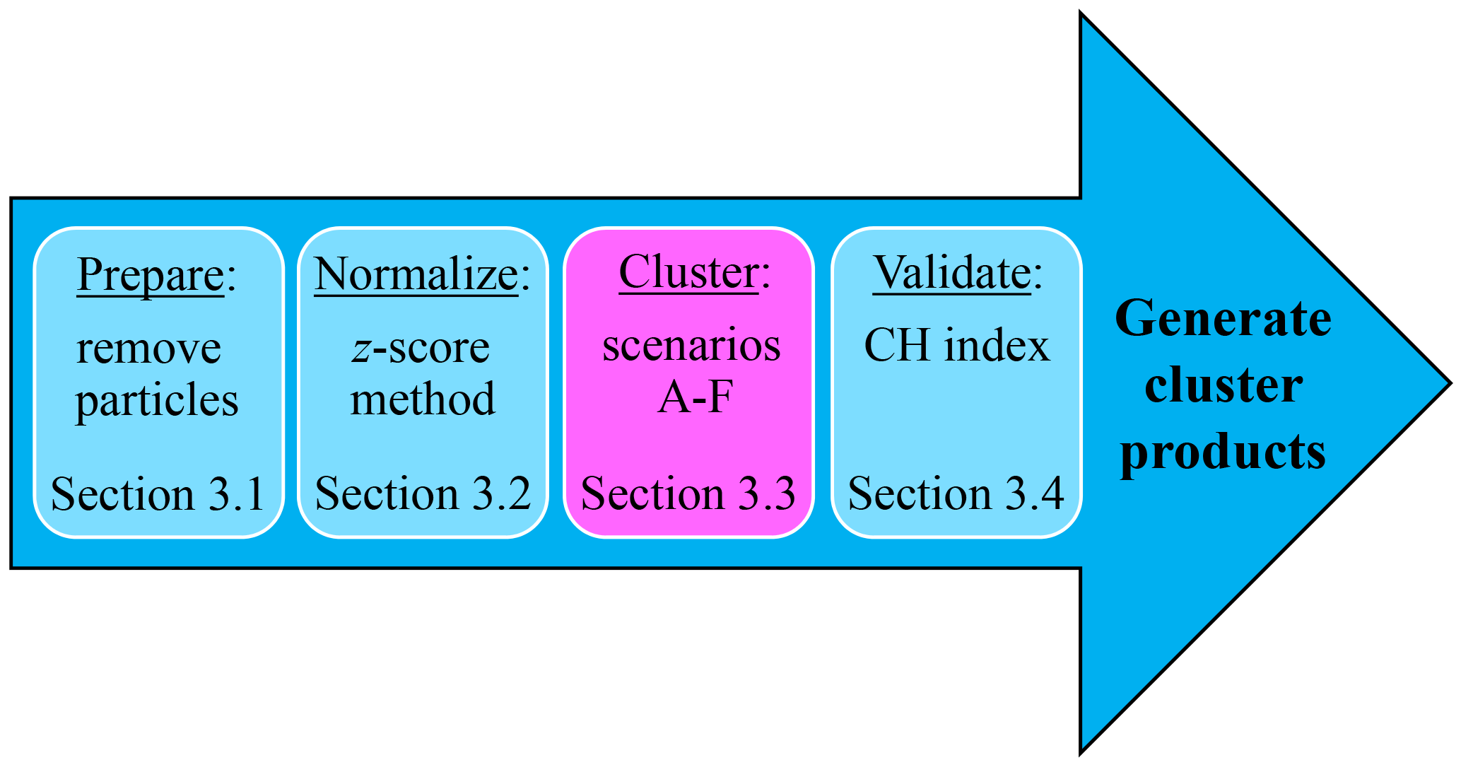
Figure 1 Schematic diagram showing the data preparation process resulting in the generated clustering products. Parameters within the pink box are the focus of this paper.

3 Clustering strategy

Hierarchical clustering methods work by grouping objects from the bottom up, meaning that each object (particle) starts as its own “cluster,” and clusters are merged together based on similarities until a greatly reduced number of clusters are presented as a final solution. Ward's method for clustering is among the most popular approaches for HAC and is the only method based on a classical sum-of-squares criterion, minimizing the within-group sum of squares (or variance) (Müllner, 2013). The WIBS-4A used here for data collection provides five parameters of information for each individual particle detected (three fluorescence channels, size, and asymmetry factor (AF)), resulting in five dimensions of data.

The clustering analysis was performed using the open-source software R package “fastercluster” (Müllner, 2013) using a Dell Latitude E7450 laptop computer with an Intel^® Core^™ Processor (i7-5600U CPU @ 2.60 GHz, 16 GB RAM).

3.1 Data preparation

Saturation of fluorescence intensity occurs at 2047 analog-to-digital counts (ADCs) for each of the three FL channels in the WIBS-4A, at which point the photomultiplier tube (PMT) reaches its upper limit of detection. A study by Ruske et al. (2017) investigated whether nonfluorescent (in that case, particles below the FT +3σ fluorescence threshold) and/or saturating data points included in the clustering analysis hindered the efficiency of the cluster output. The authors determined that removing both saturating and nonfluorescent particles before HAC analysis resulted in a better clustering performance in terms of correctly classifying ambient particles. The quality of the clustering results is likely to be impacted by the types of particles involved and the assumptions placed on those. As shown by Savage et al. (2017), many biological particles present a large fraction that saturates one or more of the fluorescence detectors. Conversely, many nonbiological particles present a large fraction of very weakly fluorescent particles with an intensity below a given threshold, which are thus classified as nonfluorescent. To limit the premodification of particle populations before clustering, the only filter applied before clustering was to remove particles smaller than the lower particle size detection limit of the WIBS-4A (0.8 µm), similar to Ruske et al. (2017). In contrast, both saturating and nonfluorescent particles were analyzed and the clustering results will be evaluated. Figure 1 outlines the data preparation process, including the conceptual process of normalization, clustering, and validation of data, which is explained in detail below.

3.2 Data normalization

Normalization of the raw data is necessary before executing the clustering algorithm because data parameters delivered from the instrument are measured on different respective scales. For example, fluorescent intensity values range from 0 to 2047 ADCs, size ranges from 0 to ∼20 µm, and AF ranges from 0 to 100 arbitrary units. Crawford et al. (2015) performed an analysis on polystyrene latex spheres (PSLs) using several different normalization techniques, concluding that z-score normalization was the best technique when looking at cluster performance using Ward's linkage for the separation of PSLs. As a result, we utilize the z-score normalization of Ward's linkage HAC for the presented study. By this type of normalization, the mean value of all data points is subtracted from each individual data point, and then each data point is divided by the standard deviation of all points. Standardization using the z-score method compares results to a normal (Gaussian) population, and we have chosen to standardize our variables to a mean of 0 and a variance of 1 so that the output variables would be on comparable scales.

3.3 HAC scenarios

Hierarchical agglomerative clustering performs optimally if all variables (1) are independent of one another and (2) can be described well by a normal (Gaussian) distribution (Norusis, 2011). To achieve meaningful results from the clustering analysis, data values must, therefore, be input into the clustering algorithm with an understanding of how specific preparatory conditions can significantly impact results. To investigate optimal input conditions, a total of six clustering scenarios was explored, with conditions summarized in Table 1. The impact of two separate variables was explored within these scenarios by varying (i) whether fluorescence intensity was pre-normalized by particle size and (ii) whether the data values were input after logarithmic transformation to produce a normal distribution.

Table 1 Six scenarios explored, with varying combinations of pre-analysis treatment. “Fluorescence normalization” refers to whether fluorescence intensity values were input to HAC as reported by the instrument (No) or after normalizing to particle size (Yes). “Variables logged” refers to whether data values were input as reported (No) or manipulated to produce a normal distribution by using log(value) (Yes).

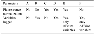
Ambient particle number vs. size distributions can often be well approximated by lognormal distributions, although specific groups of particles, including some bacteria, spores, and pollen, may not always exhibit a lognormal distribution. Further, fluorescence intensity has been shown to scale with particle size (e.g., Hill et al., 2001; Sivaprakasam et al., 2011). Several previous studies attempted to utilize HAC for ambient lognormally distributed particle size data (Crawford et al., 2014, 2015; Robinson et al., 2013) but applied the assumption that particle fluorescence is normally distributed in a group of particles. If this assumption is not correct, however, weakly fluorescing particles are likely to be grouped into a single cluster based on the high abundance of these particles (Robinson et al., 2013). Scenarios C, D, and E (Table 1) utilize data input to the clustering algorithm after fluorescence intensity was normalized to particle size (by dividing fluorescence intensity value by light scattering signal when a particle interacts with the diode laser beam) in order to explore the assumption that laboratory data should be treated like previously explored ambient data sets and not logged. Scenarios B and D take into account the logging of all parameters, producing normal distributions of all variables (AF, particle size, three channels of fluorescence). By this process, data values were input into the algorithm as a log(value) without separately binning the points. For comparison, scenarios E and F explore log-spaced distributions of size and AF, while retaining the assumption that the fluorescence output is normally distributed. Scenario A data are neither logged nor normalized. For comparison, scenario F represents the input conditions that have been used frequently (e.g., Crawford et al., 2015; Ruske et al., 2017).

3.4 Cluster validation

An important feature of HAC is that it provides clusters in an unsupervised manner, and the user must determine the number of clusters that makes physical sense. One useful tool to systematically determine the optimal number of final clusters is the Calinski–Harabasz (CH) index, which uses the interclass–intraclass distance ratio (Liu et al., 2010). For each clustering output the CH index was calculated for cluster solutions with 1 through 10 clusters, and the solution with the highest CH value was generally determined to be the optimal number of clusters. Figure 2 shows an example CH value versus cluster number plot for a mixture of Aspergillus niger fungal spores mixed with diesel soot particles. The curve suggests the optimal result to be a two-cluster solution for this trial, as was generally the case for investigations where two particle types were mixed before clustering. In order to reduce the length and complexity of discussion, the analysis of results in Sects. 4.1–4.3 was limited to using cluster products only from the two-cluster solution. In some cases, a three-cluster solution may have produced higher-quality results, but these cases were not investigated.

4 Results and discussion

The analysis of clustering quality was performed systematically and with increasing complexity. Section 4.1 utilizes three pairs of particles types to explore the effect of particle ratio and normalization strategies on cluster performance. Using conclusions from this section, Sect. 4.2 then expands the exploration to 20 additional pairs of particle types. Section 4.3 explores the effect of three different fluorescence thresholding strategies on cluster output. Finally, Sect. 4.4 investigates the ability of HAC analysis to separate particle types from mixed populations of particle types.

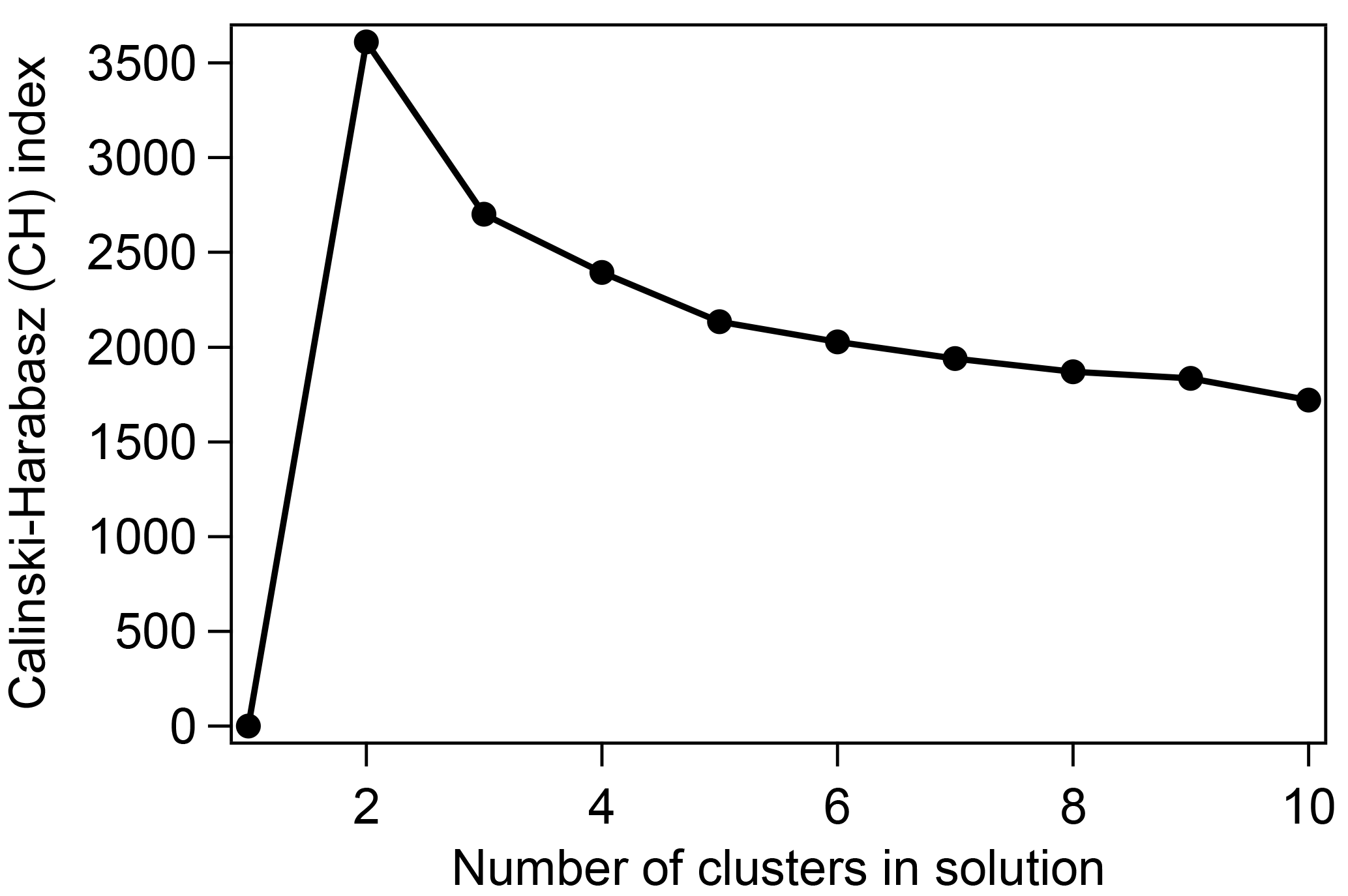
Figure 2 Example of a Calinski–Harabasz index plot for the cluster experiment with input from Aspergillus niger and diesel soot (50:50 ratio). The optimal number of clusters is determined by the highest CH value. For Sects. 4.1–4.3 only two-cluster solutions were analyzed.

4.1 Investigating pre-normalization scenarios and particle input ratio

To explore the ability to separate two distinct populations of particles from one another, three different clustering trials are presented in this section as one-to-one matchups: (1) Aspergillus niger (fungal spores, F2) vs. standard diesel soot (S4), (2) Pseudomonas stutzeri (bacteria, B3) vs. standard diesel soot (S4), and (3) Aspergillus niger (fungal spores, F2) vs. California sand (mineral dust, D12). These four particle materials were chosen to represent key classes of coarse particles observed in ambient air. For each trial, a subset of particles from each material type was selected randomly for HAC analysis. The clustering process includes (i) the evaluation of cluster performance based on particle assignment and cluster composition and (ii) the visual representations of cluster outputs using the particle type classification introduced by Perring et al. (2015). For each of these three trials, the clustering process was run separately using each of the six scenarios A–F described in Table 1. Additionally, while exploring the optimal data preprocessing scenario, the influence that different concentration ratios of particle types could play in the clustering output was also explored. The cluster process for each trial was performed using four different ratios of particles in each particle set including situations with an equal ratio and where the concentration of each particle type was significantly mismatched. In total, this section represents 57 individual clustering experiments (3 trials ×6 scenarios ×3 particle ratios +3 additional ratio trials) exploring three independent input variables. The results will be utilized to explore many more individual particle type matchups in the following sections.

The first two trials include diesel soot particles because light-absorbing carbon aerosol is commonly observed in aerosol samples with anthropogenic influence (Bond et al., 2013) and because it can have fluorescence characteristics difficult to distinguish from small biological particles (e.g., Huffman et al., 2010; Pan et al., 2012; Savage et al., 2017; Yu et al., 2016). For example, when excited by photons with a wavelength of 280 nm, diesel soot can be misinterpreted as single bacterial cells using the WIBS, and so we explored here whether the two particle types could be clustered separately (Pöhlker et al., 2012). The three trials include two examples of biological particles, both exhibiting fluorescent properties but with different excitation–emission characteristics and with a different average particle size.

The output of the algorithm reports the particle type from which each particle was input in order to evaluate the accuracy of the clustering. The resulting output of each particle with an assigned cluster number is then compared to the originating particle type to determine classification accuracy. Figure 3 summarizes the relative accuracy of individual clustering experiments by representing the percent of particles misclassified with respect to known input identities (blue bar corresponding to correct classification, red bar and overlaid value corresponding to incorrect classification). The clustering process was generally effective for separating particles correctly when two particle types were considered, but results vary widely across the six scenarios. Several previous studies that used HAC to separate particles within an ambient data set assumed that particle fluorescence is already normally distributed (Crawford et al., 2014, 2015; Robinson et al., 2013). As a result, these previous studies did not normalize fluorescence data and thus used data preparation scenario F in their clustering analysis. For comparison, scenarios B and D were explored to test whether the clustering efficiency would be improved or hindered by fluorescence normalization. Scenarios A and F produced inconsistent results, with some experiments (i.e., a 50:50 ratio of fungal spores : diesel) producing a misclassification < 1.1 %, whereas other experiments (i.e., a 20:80 ratio of bacterial : diesel) produced a misclassification of up to 80 %. In contrast, scenarios B and D produced consistently more accurate results. Scenario B, in particular, consistently exhibited the most accurate classification of particles for almost every individual experiment. No experiment involving scenario B produced a greater than 9 % misclassification of particles, regardless of the particle input ratio, and most experiments produced results with 0.1 %–3 % error. These observations taken together suggest that particle fluorescence properties may not be well described by normal distributions and that normalizing fluorescence data prior to analysis may be more effective.

Figure 3 Cluster misclassification shown for three computational combinations of fungal spores (F2), bacteria (B3), diesel soot (S4), and mineral dust (D12). Each combination explored with respect to the ratio of input particle number using scenario B and a two-cluster solution for each experiment. Scenario letters A–F refers to the scenarios summarized in Table 1. Red shaded regions (and values) indicate the percent of particles misclassified. Blue shaded regions represent the percentage of particles correctly classified.

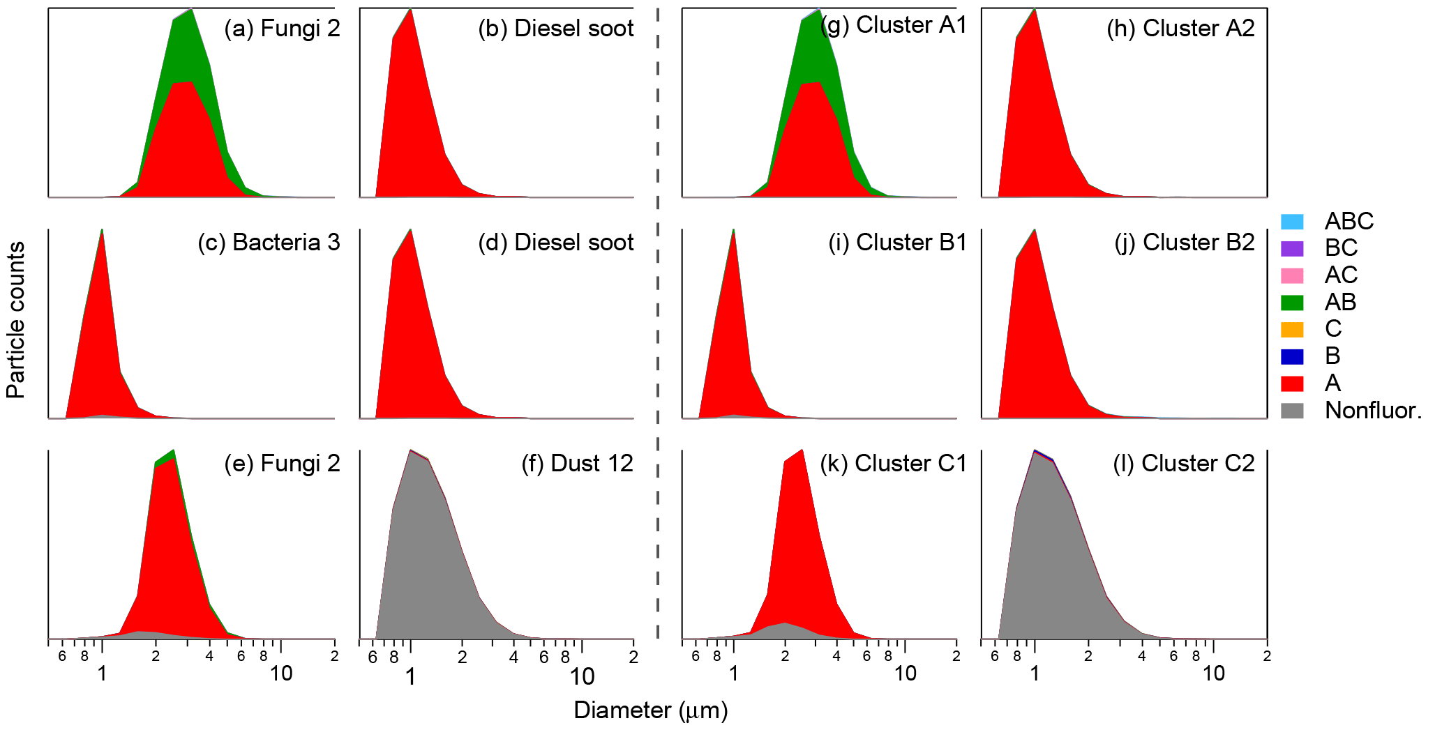
Figure 4 Particle type stacked-category size distributions for input and output clustering results, using FT +3σ threshold definition. Each experiment (row) shows matchups of two particle types computationally mixed using 50:50 ratios, scenario B, and two-cluster solutions. Panels (a)–(f) show the properties of input particles; (g)–(l) show the properties of cluster outputs.

The results of these experiments also highlight how important the ratio of input particles can be. While scenario B was relatively consistent, varying only between 0.1 % and 3.8 % error for different ratios of the fungal spore versus diesel matchup, other experiments depended strongly on particle ratio. It is clear that the input ratio of particle types cannot be controlled during an ambient study, and so these results suggest that it is important to keep the possibility of varying concentration ratios in mind when interpreting time- or air-mass-associated changes in cluster composition or when relaying the relative confidence in clustering results. For the remainder of the discussion, experiments will be limited to a 50:50 ratio following scenario B. In each case the input particles are a random subset taken from the pool of particles in the experimental data. As a result, individual samples selected from the same experiments (i.e., Fig. 4a, e) can show slightly different average properties. In some cases (i.e., diesel soot; Fig. 4d) the number of particles originally analyzed was small, and so to keep the input particle ratio at 50:50, the corresponding particle type was also limited to small numbers.

To extend the investigation of the particle input ratio, the three matchups presented in Fig. 3 were investigated using scenario B with 1 % bioparticles and 99 % non-bioparticles in each case. In these experiments the bacteria : diesel soot and fungal spores : dust particles separated relatively well (6.6 % and 13.5 % misclassification, respectively). The fungal spores : diesel soot separation was poor, however, because the diesel soot particles were nearly evenly split into both clusters, and the fungal spore particles were too low in concentration to influence the cluster properties. More investigation is needed to explore how extreme disparities in particle ratio could negatively influence cluster quality in real-world settings.

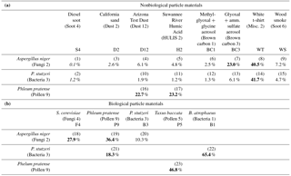
Table 2 Misclassification of two-cluster solutions for 23 matchups of two individual particle types (equal ratio of particle number, B scenario, no fluorescence threshold applied) computationally combined before clustering analysis. Misclassification calculated as the sum percentage of particles misclassified in each cluster divided by the total number of particles. Three biological particle types (F2, B3, P9) compared separately to (a) nonbiological particle materials and (b) biological particle materials. Particle number input was a subset of the total population of particles experimentally analyzed. Bold values show a misclassification > 15 %.

An important tool readily applied to the analysis of ambient data is the categorization of particles into eight fluorescent particle types (Perring et al., 2015). Thus, to further investigate the quality of cluster accuracy, Fig. 4 shows inputs and cluster outputs from three clustering experiments stacked as a function of fluorescence particle type and particle size. Figure 4a, b, g, and h show the input data for Aspergillus niger and diesel soot (Fig. 4a–b) paired with the outputs of the two-cluster solution (Fig. 4g–h). It can be seen that both particle materials have predominantly particle type A characteristics, meaning that they are fluorescent only in channel FL1. The fungal material also presents roughly one-third of AB (green) and a small minority of nonfluorescent (gray) characteristics. The size distribution of the fungal spores peaks at ∼3 µm, whereas diesel soot peaks at ∼1 µm in size. While not shown in this plot style, the spores exhibit moderately higher FL1 channel fluorescence, with a median of 543 ADCs, whereas diesel soot exhibits a median of 751 ADCs in this channel (see Savage et al., 2017; Table 2). Both particle types show almost no fluorescent characteristics in either FL2 or FL3. In summary, the particle distributions are relatively similar in fluorescence particle type and their differences are largely related to particle size, so separation of these particles through Trial 1 was hypothesized to represent a relatively challenging initial exercise. The clustering outputs presented in Fig. 4g–h, however, visually highlight the conclusion represented by Fig. 3, which is that the particles in this trial separated very well. Cluster 1 was comprised predominantly of fungal particles and presented fluorescence and size traits qualitatively similar to the input fungal particles, whereas cluster 2 was comprised predominantly of diesel soot particles.

Results from the 50:50 ratio of the scenario B experiments for the other two trials are also shown in Fig. 4c, d, i, and j and Fig. 4e, f, k, and l. In each case, the qualitative properties of the input particles are extremely well represented by the corresponding output cluster, corroborating the conclusion from Fig. 3 that the scenario B cases accurately separated the particle groups investigated through these experiments. It is also important to note here that the method of aerosolization for each particle type plays an important role in the observed size distribution, and so results involving laboratory particles should be interpreted with this in mind. Observed fluorescence properties, in contrast, are expected to be conserved at a given particle size and are intrinsically related to particle composition.

4.2 Investigating cluster quality without fluorescence threshold

After concluding that scenario B exhibited the most consistently accurate clustering results using two-cluster solutions from mixtures comprised of two particle type inputs, the analysis was expanded to include a broader range of particle types. Using 50:50 ratios of two types of input particles, prepared using scenario B (leaving fluorescence data un-normalized and logarithmically transforming data vaules), 20 new individual experiments were performed. The results of all 23 experiments (3 from Sect. 4.1 and 20 introduced in Sect. 4.2) are summarized in Table 2 as the percentage of particle misclassification. These trials were chosen to represent a broad range of individual matchups that might be expected in ambient air. Of the original 69 types of particles analyzed by Savage et al. (2017), 14 were used in experiments here: 8 types of nonbiological particles and 6 types of biological particles (2 each of fungal spores, bacteria, and pollen species). Supplement Fig. S4 from Savage et al. (2017) shows size distributions stacked by fluorescence particle type for each of the particle species discussed.

Table 2a organizes clustering results into three rows, showing the misclassification of F2 (Aspergillus niger fungal spores), B3 (Pseudomonas stutzeri bacteria), and P9 (Phelum pratense pollen) particles with respect to a variety of other particle types represented by table column. Of the 15 cluster experiments between fungal spores or bacteria and nonbiological material, only 3 showed a misclassification greater than 7.5 % (bold text) and 7 were less than 3 %. The three outliers were experiment 7 (F2 vs. BC3; glyoxal + ammonium sulfate brown carbon aerosol), 8 (F2 vs. WT; white t-shirt particles), and 14 (B3 vs. WT). Looking first at experiment 7, F2 particles show A-type fluorescence characteristics and are dominated by a mode between 1.5 and 4 µm. BC3 particles are primarily nonfluorescent < 1.5 µm but are primarily A-type between 1.5 and 3 µm, suggesting similar size and fluorescence properties. The white t-shirt particles separated poorly (∼41 % misclassification) from both the fungal spore and bacterial particles. All three particle types (WT, F2, and B3) exhibit medium fluorescent intensity in the FL1 channel. The poor ability to separate WT from both F2 and B3 was surprising, however, given that WT exhibited significantly higher mean fluorescence in each of the FL2 and FL3 channels. As first mentioned by Savage et al. (2017), great care should be taken when interpreting fluorescent particle results from indoor environments where increased concentrations of bleached fibers from clothing, bedding, paper, and cleaning products may be present.

While the results show that the fungal spores and bacterial particles investigated could generally be well separated from most potentially interfering nonbiological species, the results were much less successful for differentiation from pollen. P9 pollen particles separated poorly in all experiments (versus D12, H2, or P5), with a rate of misclassification ranging from 22 to 47 %. It is important to keep in mind, however, that the WIBS was operated using a standard gain setting that limits analysis of particle size to below approximately 20 µm. As a result, the WIBS is insensitive to whole pollen grains, and so most of the particles observed during pollen experiments are small pollen fragments. Any intact pollen grains that navigate the flow system to be detected are likely to be binned together in the channel representing the largest particles. Clustering results including pollen should be interpreted accordingly. Pollen grains can fragment in ambient air as a function of increased relative humidity (Miguel et al., 2006; Suphioglu et al., 1992; Taylor et al., 2004), but the relative ratio of whole / fragmented particles is hard to predict under ambient conditions. Smaller fragments can also exhibit different fluorescent properties to whole grains (Pöhlker et al., 2013). O'Connor et al. (2014) operated a WIBS-4 (Univ. Hertfordshire) at a lower gain in order to improve the pollen detection efficiency, but these results are not explored directly here.

The WIBS instrument is frequently used to differentiate between airborne biological particles and material of nonbiological origin. A secondary goal of differentiating more finely between types of biological aerosols is also frequently pursued. To investigate this goal, six additional experiments were conducted by pairing two different types of nonbiological particles (Table 2b). In contrast to the results shown in Table 2a, the clustering algorithm showed a generally poor ability to separate between two biological particle types. Only one of the six experiments resulted in an error < 15 % (F2 vs. B3, 10.3 % error), whereas error for the other five experiments ranged from 18 % to 65 %. The worst accuracy was demonstrated by experiment 22 (B1 vs. B3) and experiment 23 (P5 vs. P9). Both of these experiments attempted to separate between different species of a single particle type (i.e., between two bacteria or two pollen). Overall, these results suggest that the clustering strategy may be quite useful at aiding the differentiation of biological material from nonbiological material but that separating more finely to quantify differences between types of individual biological particles is significantly more challenging and not likely to be possible in most situations.

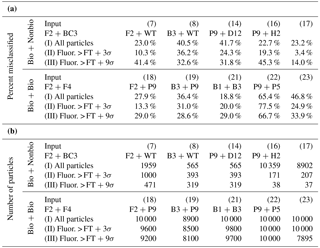
Table 3 Further exploration of two-cluster solutions for the 10 matchups of two individual particle types shown in Table 2 with a misclassification > 15 %. Each matchup is shown using three separate fluorescence threshold strategies in advance of particle input into the cluster algorithm: (I) all particles included (no fluorescence threshold), (II) particles with fluorescence intensity < FT +3σ removed, and (III) particles with fluorescence intensity < FT +9σ removed. (a) Particle misclassification. (b) Total particle number used for clustering experiment.

4.3 Investigating the impact of fluorescence thresholding strategy on cluster quality

In previously published studies, removing particles from clustering analysis that exhibited a particle fluorescence intensity below the threshold (i.e., nonfluorescent) or at the saturating point improved the efficiency of clustering (Crawford et al., 2015; Ruske et al., 2017). In Sects. 4.1–4.2, particles with either of these characteristics were left in the analysis to prevent the underestimation of the particles clustered. In this section, however, we investigated whether removing nonfluorescent particles could improve cluster accuracy for the experiments that performed poorly in Sect. 4.2. Of the 23 trials represented in Table 2, 10 experiments exhibited a 15 % or greater misclassification and were subjected to further analysis in order to investigate whether using a more discriminating fluorescence thresholding strategy could improve cluster results. In all 10 cases, fluorescence saturating particles were retained, and three separate thresholding conditions were compared by (i) keeping all nonfluorescent and saturating particles, (ii) removing nonfluorescent particles by applying a fluorescence threshold of FT baseline +3σ, and (iii) removing nonfluorescent particles by applying a fluorescence threshold of FT baseline +9σ. Savage et al. (2017) showed evidence that applying a FT +9σ improved WIBS results by removing a higher fraction of nonbiological material from analysis than the more commonly used FT +3σ, without negatively impacting observations of biological particles. Table 3 shows the percentage of particles misclassified in each of the three scenarios investigated here (Table 3a) as well as the number of particles subjected to the clustering algorithm (Table 3b).

Each scenario, with exception of the B3 vs. B9 experiment 21, shows a decrease in particle misclassification from scenario I (no fluorescence threshold applied) to scenario II (FT +3σ). In contrast, 8 of the 10 scenarios increase in particle misclassification when raising the fluorescence threshold from 3σ (II) to 9σ (III). The exceptions to this trend are experiments 8 (F2 vs. WT) and 19 (F2 vs. P9), which show a nominal improvement in error (2 %–4 % reduction) with an increased threshold. We hypothesize that the 9σ results degrade, in most cases, because the threshold becomes high enough that most weakly fluorescing particles have been removed from analysis. This reduces the ability of the cluster to group into low- and high-fluorescence categories, and so remaining particles are separated less efficiently. Secondly, removing particles at higher fluorescence thresholds leads to increasingly poor counting statistics, as represented in Table 3b by the number of particles included in each experiment. Overall, these results suggest that inputting particles into the clustering analysis with at least a nominal fluorescence threshold (i.e., FT +3σ) can improve the clustering results in many cases; however, increasing the threshold further may decrease cluster quality.

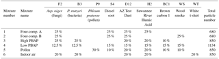
Table 4 Particle fraction for each type and total particle number used as inputs for simulated mixtures. PBAP: primary biological aerosol particle.

4.4 Investigating the capability to separate particles in simulations of complex mixtures

To this point, our investigation has focused on a variety of individual matchups between two distinct particle types. To better simulate real-world scenarios, we computationally simulated six mixtures of particles by pooling existing WIBS data from selected particle types at prescribed ratios. Each simulated mixture was assembled to roughly represent a different hypothetical mixture of particles that might be expected. Also, the particles in each simulated mixture are assumed to be so diluted that any agglomeration is negligible. Table 4 provides an overview of the percentage of each particle type included as well as the total number of particles in the mixture. Mixtures 1 and 2 were simulated arbitrarily to test if a minority (25 %) of one type of fungal spores (F2) could be separated from a majority (75 %) of a mixture of three different nonbiological materials. Mixtures 3 and 4 synthesized arbitrary mixtures of two types of bioaerosol (F2 and B3) with three or five types of nonbiological particles, respectively. Mixture 5 was simulated to examine the separation of pollen (P9) from a set of five nonbiological particles. Mixture 6 was simulated to be similar to an indoor environment that might have a mixture of biological particles (F2 and B3) with nonbiological materials, including bleached fibers (WT). These mixtures are not intended to closely mimic any set of individual ambient conditions but are rather used as very rough simulations for discussion and to prompt discussion related to future experiments within the community. In a real-world sampling environment, one would also expect a high concentration of nonfluorescent particles (e.g., most organic aerosols, sea salt, dusts), but these were generally not sampled as a part of the Savage et al. (2017) study, which focused on fluorescent particles. As a result, relatively nonfluorescent particles like D12 and H2 were included here as “fillers” in most mixtures as surrogates for other types of nonfluorescent particles. Clustering analysis was performed using the ratios listed in Table 4, the B scenario of pre-normalization conditions, and the filtering of nonfluorescent particles below the FT +3σ threshold. In all cases, the number of clusters retrieved after HAC was pre-defined to be the same as the number of particle types input.

Figure 5 Overview of computationally simulated mixtures. Six mixtures shown as groups of rows, with input particle fractions defined in Table 4. Panel (a)  shows the particle number retrieved by each individual cluster (horizontal rows) categorized by each input particle type (vertical columns). Panel (b) shows the particle number categorized and grouped by particle classes (i.e., nonbiological and biological). Panel (c) shows the misclassification of groups of particles. Colors: light green – fungal spores; blue – bacteria; pink – pollen; dark green – grouped biologically; brown – all nonbiological.

Cluster results from all six mixtures are summarized in Fig. 5. Figure 5a shows the number of particles from each type assigned to each cluster, and panels (b) and (c) show results grouped by general particle classification (brown for nonbiological and dark green for biological). Overall, the ability of the HAC analysis to separate the biological particles from the nonbiological particles was high. In some cases, the quality of separation of one or two biological species from a mixture of nonbiological materials was even higher than the two-material matchups shown in Sects. 4.1–4.3. The two four-component mixtures showed a 22.4 % and 14.8 % misclassification of fungal spores. In both cases, a small fraction of each of the nonbiological materials was mixed into the spore cluster, whereas almost none (1.5 % and 0.6 %) of the spores were incorrectly mixed into the sum of the nonbiological clusters.

Mixtures 3 and 4 showed a similar misclassification for fungal spores (11.9 % and 13.8 %, respectively), whereas the bacterial particles clustered with amazing quality. For Mixture 3, no particles other than bacterial particles were grouped into Cluster 1, and only 16 of 213 bacterial particles were assigned to other clusters. For Mixture 4, 135 of 137 particles in Cluster 6 were bacterial in origin and 135 of 142 bacterial particles were assigned to the cluster. The combination of fungal and bacterial particles in mixtures 3 and 4 resulted in a total of 5.0 % and 5.3 % misclassification of all biological particles.

In contrast to the poor separation of pollen from other particle types discussed in Sect. 4.2, Mixture 5 showed a higher quality of separation between pollen (9.4 % misclassified) and the sum of five other nonbiological particle types. Lastly, the mixture designed to roughly mimic an indoor environment included white t-shirt particles. In this mixture the WT particles confounded the spore separation, but the bacterial separation was nearly flawless.

Another surprising observation from the analysis of these simulated mixtures was that the diesel soot particles (mixtures 1, 2, 4, and 5) separated into their own cluster in almost all cases with very high quality (1.8 %, 2.9 %, 0.6 %, and 9.4 %, respectively, of diesel soot particles misclassified into a different cluster). The quality of the separation of bacterial particles and diesel soot (Mixture 4) was especially good, given the qualitative similarity of the two particle populations. For example, size distributions of each particle type show primarily A-type particles with similar mean fluorescent intensity values in FL1, FL2, and FL3 (Savage et al., 2017).

5 Conclusions

The application of results from a recent set of systematic laboratory experiments (Savage et al., 2017) by the commonly used hierarchical agglomerative clustering analysis helps to reveal areas where the tool can be used well and other areas where it struggles. First (Sect. 4.1) it was observed that differing ratios of particle input into the clustering algorithm can produce dramatically different results. It will be important for anyone applying HAC to ambient particle sets, where particle ratios are not independently verified, to interpret results somewhat loosely. In Sect. 4.1 the clustering quality of scenario B, where fluorescence intensity was not normalized to particle size and where all variables were input in logarithmic space as log(value), was determined to consistently demonstrate the highest-quality results. Further, the ability of the HAC analysis to separate between two groups of individual particle types using no fluorescence threshold (Sect. 4.2) and comparing three separate threshold strategies (Sect. 4.3) was shown to be relatively high in many cases but confounded in others. Lastly, Sect. 4.4 explored the ability of HAC analysis to separate biological components from more complex mixtures of four to seven types of input particles.

A standard fluorescence threshold of FT +3σ has been commonly applied during WIBS analysis to separate between fluorescent and nonfluorescent particles. Savage et al. (2017) concluded that the application of a more aggressive threshold strategy (FT +9σ) could help discriminate between biological and nonbiological particles more successfully in many circumstances; however, certain types of interfering, nonbiological particle species can still confound WIBS analysis, irrespective of the threshold. Here we have investigated an orthogonal strategy to separate particle types by subjecting particles to HAC computer analysis. By comparing the results of the HAC analysis with raw separation based on fluorescence thresholding alone, the HAC analysis can clearly increase the quality of differentiation. Interestingly, while Savage et al. (2017) reported that the FT +9σ strategy helped improved differentiation, using the same threshold in conjunction with HAC analysis actually degraded results. We therefore conclude that if HAC analysis is to be performed, the standard FT +3σ threshold is likely to produce the highest-quality results; however, if HAC is not to be applied, the FT +9σ threshold is probably a better choice to enable the investigation of biological particles while computationally filtering nonbiological particles.

The overall message here is that HAC can be applied successfully to differentiate particle types sampled by WIBS instruments and that it is most successful at separating biological species (i.e., fungal spores and bacteria) from nonbiological particles. In all cases the HAC method allows the separation of particles at least at the order-of-magnitude level and often with a misclassification of < 5 %. As mentioned by Savage et al. (2017), however, it should always be kept in mind that different instruments may produce slightly different signals due to physical differences between instruments (i.e., fluorescence calibration, tuning, and detector gain sensitivity) and between calibration strategies (Könemann et al., 2018; Robinson et al., 2017). Results here are also generally extendable to other UV-LIF instruments, whether they offer single or many channels of emission spectral resolution, in that the methods of particle pre-preparation and the impact of the particle number ratio are likely to relay similar effects to the clustering strategy. Subtle differences in particles observed in a real-world environment will also complicate HAC analysis or the extension of results presented here. The UV-LIF community is encouraged to continue laboratory investigations, including a detailed interrogation of clustering analytical techniques, to further understand limitations to better differentiating between particles.