the Creative Commons Attribution 4.0 License.
the Creative Commons Attribution 4.0 License.
 | 28 Feb 2019
Spectral Intensity Bioaerosol Sensor (SIBS): an instrument for spectrally resolved fluorescence detection of single particles in real time
Tobias Könemann
Nicole Savage
Thomas Klimach
David Walter
Janine Fröhlich-Nowoisky
Ulrich Pöschl
Primary biological aerosol particles (PBAPs) in the atmosphere are highly relevant for the Earth system, climate, and public health. The analysis of PBAPs, however, remains challenging due to their high diversity and large spatiotemporal variability. For real-time PBAP analysis, light-induced fluorescence (LIF) instruments have been developed and widely used in laboratory and ambient studies. The interpretation of fluorescence data from these instruments, however, is often limited by a lack of spectroscopic information. This study introduces an instrument – the Spectral Intensity Bioaerosol Sensor (SIBS; Droplet Measurement Technologies (DMT), Longmont, CO, USA) – that resolves fluorescence spectra for single particles and thus promises to expand the scope of fluorescent PBAP quantification and classification.
The SIBS shares key design components with the latest versions of the Wideband Integrated Bioaerosol Sensor (WIBS) and the findings presented here are also relevant for the widely deployed WIBS-4A and WIBS-NEO as well as other LIF instruments. The key features of the SIBS and the findings of this study can be summarized as follows.
-
Particle sizing yields reproducible linear responses for particles in the range of 300 nm to 20 µm. The lower sizing limit is significantly smaller than for earlier commercial LIF instruments (e.g., WIBS-4A and the Ultraviolet Aerodynamic Particle Sizer; UV-APS), expanding the analytical scope into the accumulation-mode size range.
-
Fluorescence spectra are recorded for two excitation wavelengths (λex=285 and 370 nm) and a wide range of emission wavelengths (λmean=302–721 nm) with a resolution of 16 detection channels, which is higher than for most other commercially available LIF bioaerosol sensors.
-
Fluorescence spectra obtained for 16 reference compounds confirm that the SIBS provides sufficient spectral resolution to distinguish major modes of molecular fluorescence. For example, the SIBS resolves the spectral difference between bacteriochlorophyll and chlorophyll a and b.
-
A spectral correction of the instrument-specific detector response is essential to use the full fluorescence emission range.
-
Asymmetry factor (AF) data were assessed and were found to provide only limited analytical information.
-
In test measurements with ambient air, the SIBS worked reliably and yielded characteristically different spectra for single particles in the coarse mode with an overall fluorescent particle fraction of ∼4 % (3σ threshold), which is consistent with earlier studies in comparable environments.
- Article
(8093 KB) - Full-text XML
-
Supplement
(12689 KB) - BibTeX
- EndNote


Aerosol particles are omnipresent in the atmosphere, where they are involved in many environmental and biogeochemical processes (e.g., Baron and Willeke, 2001; Després et al., 2012; Fuzzi et al., 2006; Hinds, 1999; Pöschl, 2005; Pöschl and Shiraiwa, 2015). Primary biological aerosol particles (PBAPs), also termed bioaerosols, represent a diverse group of airborne particles consisting of whole or fragmented organisms including, e.g., bacteria, viruses, archaea, algae, and reproductive units (pollen and fungal spores), as well as decaying biomass (e.g., Deepak and Vali, 1991; Després et al., 2012; Fröhlich-Nowoisky et al., 2016; Jaenicke, 2005; Madelin, 1994; Pöschl, 2005) and can span sizes from a few nanometers up to ∼100 µm (Hinds, 1999; Schmauss and Wigand, 1929). Increasing awareness of the importance of PBAPs regarding aerosol–cloud interactions, health aspects, and the spread of organisms on local, continental, or even intercontinental scales has led to growing interest by scientific researchers and the public (e.g., Després et al., 2012; Fröhlich-Nowoisky et al., 2016; Yao, 2018).
Due to the inherent limitations (e.g., poor time resolution and costly laboratory analyses) of traditional off-line techniques (e.g., light microscopy and cultivation-based methods) for PBAP quantification, several types of real-time techniques have been developed within the last several decades to provide higher time resolution and lower user costs (e.g., Caruana, 2011; Després et al., 2012; Fennelly et al., 2017; Ho, 2002; Huffman and Santarpia, 2017; Jonsson and Tjärnhage, 2014; Sodeau and O'Connor, 2016). One promising category of real-time instruments – meaning that particles are sampled and analyzed both instantly and autonomously – involves the application of light-induced fluorescence (LIF). The main principle of this technique is the detection of intrinsic fluorescence from fluorophores ubiquitous in biological cells, such as those airborne within PBAPs. These fluorophores include a long list of biological molecules such as aromatic amino acids (e.g., tryptophan and tyrosine), coenzymes (e.g., reduced pyridine nucleotides (NAD(P)H)), flavin compounds (e.g., riboflavin), biopolymers (e.g., cellulose and chitin), and chlorophyll (e.g., Hill et al., 2009; Li et al., 1991; Pan et al., 2010; Pöhlker et al., 2012, 2013). Detailed information on biological fluorophores can be found elsewhere (Pöhlker et al., 2012, and references therein).
Today, commercial online LIF instruments such as the Ultraviolet Aerodynamic Particle Sizer (UV-APS; TSI Inc. Shoreview, MN, USA) and the Wideband Integrated Bioaerosol Sensor (WIBS; developed by the University of Hertfordshire, UK, and currently licensed and manufactured by Droplet Measurement Technologies, Longmont, CO, USA) are commonly applied for research purposes. Detailed descriptions of the UV-APS (e.g., Agranovski et al., 2003; Brosseau et al., 2000; Hairston et al., 1997) and the WIBS series (e.g., Foot et al., 2008; Kaye et al., 2000, 2005; Stanley et al., 2011) are given elsewhere. Concisely, the UV-APS uses an λex=355 nm laser excitation source and spans an emission range of λem=420–575 nm. In contrast, the WIBS applies two pulsed xenon flash lamps emitting at λex=280 and 370 nm, whereas fluorescence emission is detected in three detection channels, λem=310–400 nm (at λex=280 nm), and λem=420–650 nm (at λex=280 and 370 nm). Both instruments provide spectrally unresolved fluorescence information, which means that fluorescence is recorded in, e.g., one to three integrated and spectrally broad channels. The latest WIBS model is currently the WIBS-NEO, whose design is based on a WIBS-4A but with an extended particle size detection range between ∼ 500 nm and 30 µm (nominal). Both UV-APS and WIBS models have been examined in a variety of laboratory validations (e.g., Agranovski et al., 2003, 2004; Brosseau et al., 2000; Healy et al., 2012; Hernandez et al., 2016; Kanaani et al., 2007; O'Connor et al., 2013; Saari et al., 2013, 2014; Savage et al., 2017; Toprak and Schnaiter, 2013) and have been deployed to investigate both indoor and outdoor atmospheric aerosol via longer-term measurements (e.g., Bhangar et al., 2014; Calvo et al., 2018; Crawford et al., 2016; Fernández-Rodríguez et al., 2018; Foot et al., 2008; Gabey et al., 2010, 2013; Gosselin et al., 2016; Healy et al., 2014; Huffman et al., 2010, 2012, 2013; Ma et al., 2019; Perring et al., 2015; Schumacher et al., 2013; Twohy et al., 2016; Ziemba et al., 2016).
Although LIF instruments do not offer the same qualitative ability to identify sampled particles as, e.g., off-line microscopy, mass spectrometry, or culture-based methods, they provide size-resolved information as well as fast sampling and fine-scale temporal information for single particles not accessible with off-line techniques. Nevertheless, these instruments present significant challenges. For example, the quantification of PBAPs by LIF instruments is hindered by the fact that some biological materials reveal weak fluorescence characteristics that do not rise above detection thresholds (Huffman et al., 2012). In addition to this complication, the detection threshold is not a universally defined parameter and varies for each channel between different units of the same type of instrument (e.g., Hernandez et al., 2016; Savage et al., 2017). Furthermore, the unambiguous spectroscopic characterization of bioparticles is fundamentally challenging because fluorescence spectra of even individual molecules in condensed matter are relatively broad due to radiative decay pathways of excited electrons. Further, bioparticles are chemically complex, each comprised of a mixture of at least dozens of types of fluorophores that can each emit a unique emission spectrum that smears together with others into an even broader fluorescence spectrum from each particle (Hill et al., 2009, 2015; Pan, 2015). Another difficulty is that many nonbiological particles, such as certain mineral dusts and polycyclic aromatic hydrocarbons (PAHs), may fluoresce, making it more difficult to distinguish patterns arising from biological particles (e.g., Pöhlker et al., 2012, and references therein; Savage et al., 2017). Lastly, most currently available commercial LIF instrumentation is limited to recording data in one to three spectrally integrated emission channels, which limits the interpretation of fluorescence information. Recent efforts to apply more complex clustering algorithms to spectrally unresolved WIBS-type data are proving helpful at adding additional discrimination (e.g., Crawford et al., 2015; Robinson et al., 2013; Ruske et al., 2017; Savage and Huffman, 2018). For example, it was shown for a rural forest study in Colorado that a cluster derived using WIBS-3 data, assigned to fungal spores (Crawford et al., 2015), correlated well with the mass concentration of molecular fungal tracers (e.g., arabitol and mannitol) measured with off-line chemical techniques (Gosselin et al., 2016). In contrast, the clusters in the same study that were assigned to bacteria correlated only poorly with endotoxins used as bacterial molecular tracers (Gosselin et al., 2016). This provides evidence of a limitation to using LIF instrumentation with low spectral resolution to separate or identify some PBAP types. Additionally, the bacterial cluster allocation might have also been hampered in that case by the minimum detectable particle size of the WIBS (∼0.8 µm), resulting in a lower detection efficiency for bacteria.
The evolution of LIF techniques over the last several decades has significantly expanded our knowledge of spatiotemporal patterns of PBAP abundance in the atmosphere. Nevertheless, to further improve the applicability of LIF instrumentation to widespread PBAP detection, it is necessary both to design LIF instruments with adequate instrumental properties (e.g., high spectral resolution) and to standardize their operation by characterizing instruments thoroughly with known standards (Robinson et al., 2017). Working toward this goal, a number of LIF instruments have been developed to analyze single bioparticles by collecting resolved fluorescence spectra (e.g., Hill et al., 1999; Pan et al., 2010, 2003; Pinnick et al., 2004; Ruske et al., 2017); however, relatively little has been done to offer these commercially. Examples of commercially available instruments providing resolved fluorescence spectra are the PA-300 (λex=337 nm; λem=390–600 nm, 32 fluorescence detection channels) (Crouzy et al., 2016; Kiselev et al., 2011, 2013) and the follow-up model Rapid-E (λex=337 nm; λem=350–800 nm, 32 fluorescence detection channels) (http://www.plair.ch/, last access: October 2018), both manufactured by Plair SA, Geneva, Switzerland. In addition to collecting resolved fluorescence spectra, both instruments also provide measurements of the decay of fluorescence signals, also referred to as fluorescence lifetime.
Introduced here is an instrument for the detection and characterization of individual particles: the Spectral Intensity Bioaerosol Sensor (SIBS, Droplet Measurement Technologies). The technical properties of the instrument are described in detail and its performance is validated with sizing and fluorescence particle standards, as well as with particles in ambient air. Due to the dual excitation and spectrally resolved fluorescence in combination with a broad size detection range, the SIBS has the potential to increase the selectivity of fluorescent biological and nonbiological particle detection and discrimination. Because the SIBS uses a comparable optical system as the WIBS-4A and WIBS-NEO, the technical details presented here are broadly important to a growing community of scientists investigating both indoor and outdoor aerosol. The insights and data presented will thus contribute to ongoing discussions within the community of LIF users and will also stimulate discussions about needs for future instrument improvements.
2.1 Chemicals and materials
Table S1 in the Supplement summarizes 19 polystyrene latex spheres (PSLs, 5 doped with fluorescent dye) and 6 polystyrene divinylbenzene (PS-DVB) particles, which were purchased from Thermo Fisher (Waltham, MA, USA), Bangs Laboratories Inc. (Fishers, IN, USA), Duke Scientific Corp. (Palo Alto, CA, USA), and Polysciences Inc. (Warrington, PA, USA). A detailed study regarding the steady-state fluorescence properties of PSLs and PS-DVB particles used within this study can be found in Könemann et al. (2018). Additionally, we analyzed particles comprised separately of seven pure biofluorophores (tyrosine, tryptophan, NAD, riboflavin, chlorophyll a and b, and bacteriochlorophyll) (Table S2) as well as one microorganism (Saccharomyces cerevisiae; baker's yeast, bought at a local supermarket). Table S2 also includes reference particles used for asymmetry measurements, namely iron oxide (Fe3O4), carbon nanotubes, and ammonium sulfate. Ultrapure water (MilliQ, 18 MΩ) and ≥99.8 % ethanol (CAS no. 64-17-5; Carl Roth GmbH and Co. KG, Karlsruhe, Germany) were used as solvents.
2.2 Aerosolization of reference particles
PSLs were aerosolized from aqueous suspensions with a portable aerosol generator (AG-100; DMT). For both fluorescent and nonfluorescent PSLs, one drop of the suspension (or alternatively three drops for 3 and 4 µm PSLs) was diluted into 10 mL of ultrapure water in plastic medical nebulizers (Allied Healthcare, St. Louis, MO, USA). The majority of water vapor from the aerosolization process condenses inside the mixing chamber (∼570 cm3) of the aerosol generator. By using a temperature and relative humidity (RH) sensor (MSR 145 data logger, MSR Electronics GmbH, Seuzach, Switzerland) monitoring the flow directly after the aerosol generator, we measured RH values of ∼33 % (sample flow: 1.4 L min−1, dilution: 5 L min−1), ∼39 % (sample flow: 1.4 L min−1, dilution: 4 L min−1), and ∼54 % (sample flow: 2.3 L min−1, dilution: 2 L min−1). Because of the sufficiently low RH measured, we did not use additional drying (e.g., diffusion dryer) to decrease humidity in the sample flow. Hence, the outlet of the aerosol generator was directly connected to the SIBS inlet with ∼30 cm of conductive tubing (1∕4 inch). PSLs were measured for 1 min. Nonfluorescent 4.52 µm PSLs were measured for 2 min because of the low number concentrations due to poor aerosolization efficiency and gravitational settling of larger particle sizes.
S. cerevisiae was analyzed using a method similar to the one stated above, with the exceptions that the suspension was prepared with a spatula tip of material mixed into ultrapure water and that a diffusion dryer (20 cm, 200 g silica) was added to remove excess water vapor. S. cerevisiae was measured for 5 min. Chlorophyll a and b and bacteriochlorophyll samples were diluted in 10 mL of ethanol. Between each measurement, the setup was cleaned by aerosolizing ultrapure water for 5 min.
PS-DVB particles and biofluorophores (Tables S1 and S2) were aerosolized in a dry state. For this purpose, air at a flow rate of ∼0.6 L min−1 was sent through a HEPA filter into a 10 mL glass vial. A small amount of each solid powder sample (∼1 g) was placed inside the vial and entrained into the particle-free airstream. Additionally, the sample was physically agitated by tapping the vial. The outlet was connected with ∼20 cm conductive tubing to the inlet of the SIBS. The tubing and glass vial were cleaned after each measurement to prevent particle contamination from previous measurements. Each powder was sampled until cumulative number concentrations >5000 particles were reached.
In contrast to monodisperse and spherical PSL standards, the biofluorophore aerosolization process provided a polydisperse and morphologically heterogeneous particle distribution with significant particle fractions at sizes <1 µm. Therefore, we only used particles in a size range between 1 and 2 µm with sufficient fluorescence intensity values for subsequent data analysis. The only exceptions are the chlorophyll types, for which a size range between 0.5 and 2 µm (chlorophyll a and b) and 0.5 and 1 µm (bacteriochlorophyll) was used due to a less efficient particle aerosolization.
The fluorescent background of the SIBS was measured daily by firing the xenon lamps into the optical chamber in the absence of particles (forced trigger mode). In this case, the diaphragm pump was turned off and the inlet blocked to prevent particles from reaching the optical chamber. One forced trigger mode was performed per day with 100 xenon shots per minute over a duration of 5 min. The average background signal (+1σ standard deviation, SD) was subtracted from the derived fluorescence emission of each sample. Additionally, the background signal was reviewed periodically between each biofluorophore measurement to verify that, e.g., optical components were not coated with residue from previous measurements. No significant changes in background signal were observed between individual measurements. Optimization of the thresholding strategy is still ongoing work and includes, for example, investigating whether the often applied 3σ threshold used for the WIBS (e.g., Gabey et al., 2010) also works well with respect to the optical setup of the SIBS. For the assessment of the accuracy of measured fluorescence emissions from reference compounds, a threshold of 1σ was used here.
For particle asymmetry measurements, iron (II, III) oxide (Fe3O4), carbon nanotubes, and ammonium sulfate were aerosolized in dry state, and 2 µm nonfluorescent PSLs and ultrapure water were aerosolized with the aerosol generator method outlined above with SIBS integration times of 3 min in all cases. Due to the broad distribution of asymmetry factor (AF) values for particles below 1 µm, only the size fraction ≥1 µm was used for subsequent analyses. Furthermore, we observed that AF bins between 0 and 1 and AF bin 100 tend to produce increased signal responses, especially for high particle concentrations, for which they were discarded within the analyses. The origin of this effect is unknown. However, one explanation could be optical coincidences caused by high particle concentrations, resulting in multiple particles being simultaneously present within the scattering volume, as reported by Cooper (1988) using forward-scattering signatures of cloud probes.
For the collection of particles for microscopy measurements, the sample flow was bypassed and led through a custom-made particle impactor, which was connected to a mass flow controller (D-6321-DR; Bronkhorst High-Tech B.V., Ruurlo, the Netherlands) and a membrane pump (N816.1.2KN.18; KNF, Freiburg, Germany). Particles were collected out of the sample flow onto glass coverslips (15 mm diameter) at a flow rate of 2 L min−1 over a duration of 1 min.
2.3 Reference fluorescence spectra
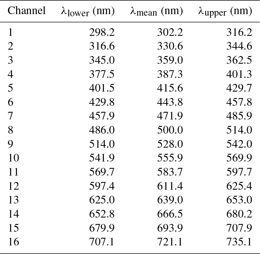
A Dual-FL fluorescence spectrometer (Horiba Instruments Incorporated, Kyoto, Japan) was used as an off-line reference instrument to validate the SIBS spectra. Aqualog V3.6 (Horiba) software was used for data acquisition. The spectrometer was manufacturer-calibrated with NIST fluorescence standard reference materials (SRMs 2940, 2941, 2942, and 2943). The aforementioned standard fluorophores were analyzed using the SIBS excitation wavelengths λex=285 and 370 nm. The Dual-FL1 spectrometer uses a xenon arc lamp as an excitation source and a CCD (charge-coupled device) as an emission detector capable of detecting fluorescence emission between 250 and 800 nm. Unless otherwise stated, a low detector gain setting (2.25 e− count−1) and an emission resolution of 0.58 nm were used for all measurements with the Dual-FL. Subsequently, we use the term “reference spectra” for all measurements performed with the Dual-FL. In total, 100 individual spectra were recorded for each sample and averaged spectra were analyzed in Igor Pro (Wavemetrics, Lake Oswego, Oregon, USA). Background measurements (solvent in the absence of particles) were taken under the same conditions as for sample measurements and subtracted from the emission signal. For direct comparison to spectra recorded by the SIBS, reference spectra were re-binned by taking the sum of the fluorescence intensity within the spectral bin width of each SIBS detection channel (Table 1).
Table 1Lower, mean, and upper wavelength at each PMT detection channel. Nominal data according to the manufacturer Hamamatsu.
For PSL measurements, 1.5 µL of each PSL stock solution was diluted in 3.5 mL of ultrapure water in a mm UV quartz cuvette (Hellma Analytics, Müllheim, Germany) and constantly stirred with a magnetic stirrer to avoid particle sedimentation during measurements. Chlorophyll a and b and bacteriochlorophyll were handled equally; however, concentrations were individually adjusted to prevent the detector from being saturated and to avoid self-quenching or inner filter effects (Sinski and Exner, 2007). Concentrations were used as follows: chlorophyll a: 300 nmol L−1, chlorophyll b: 1 µmol L−1, and bacteriochlorophyll: 3 µmol L−1. PSLs, chlorophyll b, and bacteriochlorophyll measurements were performed with an integration time of 2 s. For chlorophyll a an integration time of 1 s was used.
All other biofluorophores, S. cerevisiae, and PS-DVB particles were measured in dry state using a front surface accessory (Horiba). The sample was placed into the surface holder and covered with a synthetic fused silica window. To limit detector saturation from more highly fluorescent particle types, the surface holder was placed at a 70∘ angle to the fluorescence detector for NAD and riboflavin, 75∘ for tyrosine, 80∘ for S. cerevisiae, and 85∘ for tryptophan and PS-DVB particles and subsequently excited at λex=285 and 370 nm. Emission resolution and detector gain settings were used as for measurements of samples in solution, except for an integration time of 1 s for all dry samples. Background measurements were performed as described above and subtracted from each sample. Excitation–emission matrices (EEMs) were measured with the same samples as for single wavelength measurements. EEMs were recorded at excitation wavelengths between λex=240 and 800 nm (1 nm increments) and an emission range between λem=247 and 829 nm (0.58 nm increments). Exposure times of 1 s were used, except for 2 µm green, 3 µm nonfluorescent PSLs (2 s), and NAD (0.5 s). EEMs were analyzed using Igor Pro.
2.4 Calibration lamps and spectral correction
The relative responsivity of a fluorescence detector can vary substantially across its emission range and therefore must be spectrally corrected as a function of emission wavelength (e.g., DeRose, 2007; Lakowicz, 2004). For spectral correction it was important to choose (i) light sources covering the full spectral emission range of the SIBS, with temporal stability on the timescale of many months, and (ii) a calibrated and independent spectrometer to serve as a spectral reference.
A deuterium–halogen lamp (DH-Mini; Ocean Optics, Largo, FL, USA) and a halogen projector lamp (EHJ 24 V, 250 W; Ushio Inc., Tokyo, Japan) were used as calibration light sources. Both lamps were connected to a 50 cm optical fiber (FT030; Thorlabs, Newton, NJ, USA) and vertically fixed inside the optical chamber of the Dual-FL spectrometer. An aluminum mirror was attached to the end fitting of the optical fiber, reflecting light in a 90∘ angle into the detector opening. The projector halogen lamp was allowed to warm up for 30 s before each measurement. For all power levels (100, 150, 200, and 250 W), an integration time of 3 s was used. The DH-Mini was operational for 30 min before each measurement. Settings were used as for the projector halogen lamp; however, due to the low emission a high detector gain setting (9 e− count−1) was used with an integration time of 25 s. As described in Sect. 2.3, 100 single measurements were taken and averaged (Fig. S1 in the Supplement). For the SIBS, both light sources were measured in the same way as for the reference spectra. Measurements were performed with a detector amplification at 610 V (see Sect. 4.2). Background measurements were taken as described in Sect. 2.2. Projector halogen lamp spectra (at all power levels) were recorded for 3 min and the DH-Mini, due to its low emission intensity, for a duration of 5 min.
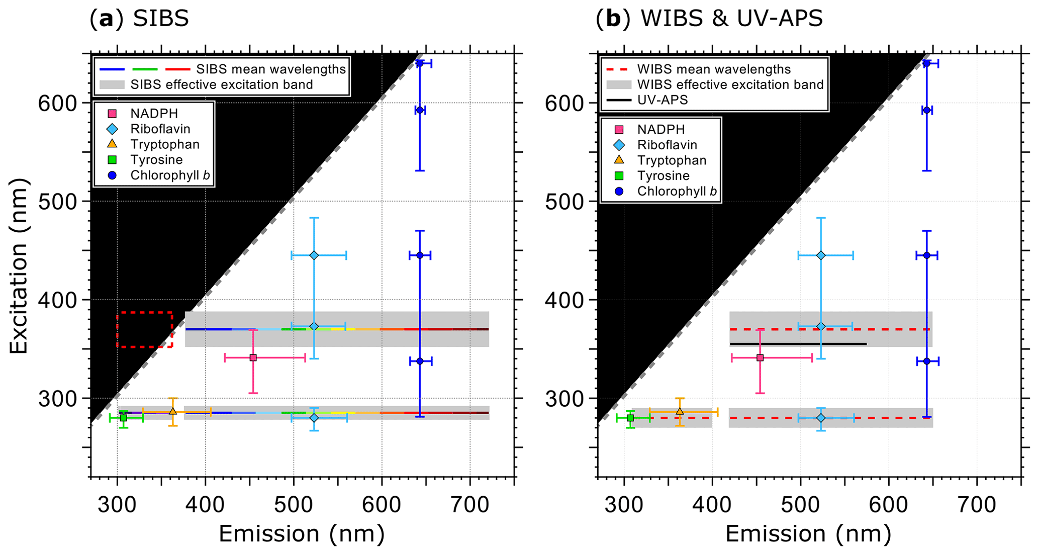
Figure 1Optical design and overview of excitation and emission specifications of the LIF instruments UV-APS, WIBS, and the SIBS with the spectral locations of the autofluorescence modes for the biofluorophores tyrosine, tryptophan, NAD(P)H, riboflavin, and chlorophyll b (as examples). Here the term WIBS includes the WIBS-4A and WIBS-NEO because both instruments use the same optical components. Spectral properties of the emission bands of LIF instruments are illustrated as horizontal lines. The color-coded bars in (a) illustrate the spectrally resolved fluorescence detection of the two excitation wavelengths (λex=285 and 370 nm) by the SIBS. The “blind spot” (white notch) at λex=285 nm at λem=362–377 nm (a) originates from a notch optical filter used to block incident light from the excitation sources. Gray dashed lines show the first-order elastic scattering. At λex=370 nm, the detection range of the SIBS includes the spectral range over which λem<λex, for which fluorescence is not defined and so data within the red dashed rectangle are omitted (a). Gray bars indicate the effective excitation bands of optical filters used for the WIBS and SIBS (see also Sect. 3.3 and Fig. 3). The effective excitation bands in the WIBS and SIBS occur in a spectral range spanning several nanometers (up to 36 nm) in contrast to the UV-APS (black line, b), which uses a laser source with a defined excitation (figure adapted from Pöhlker et al., 2012).
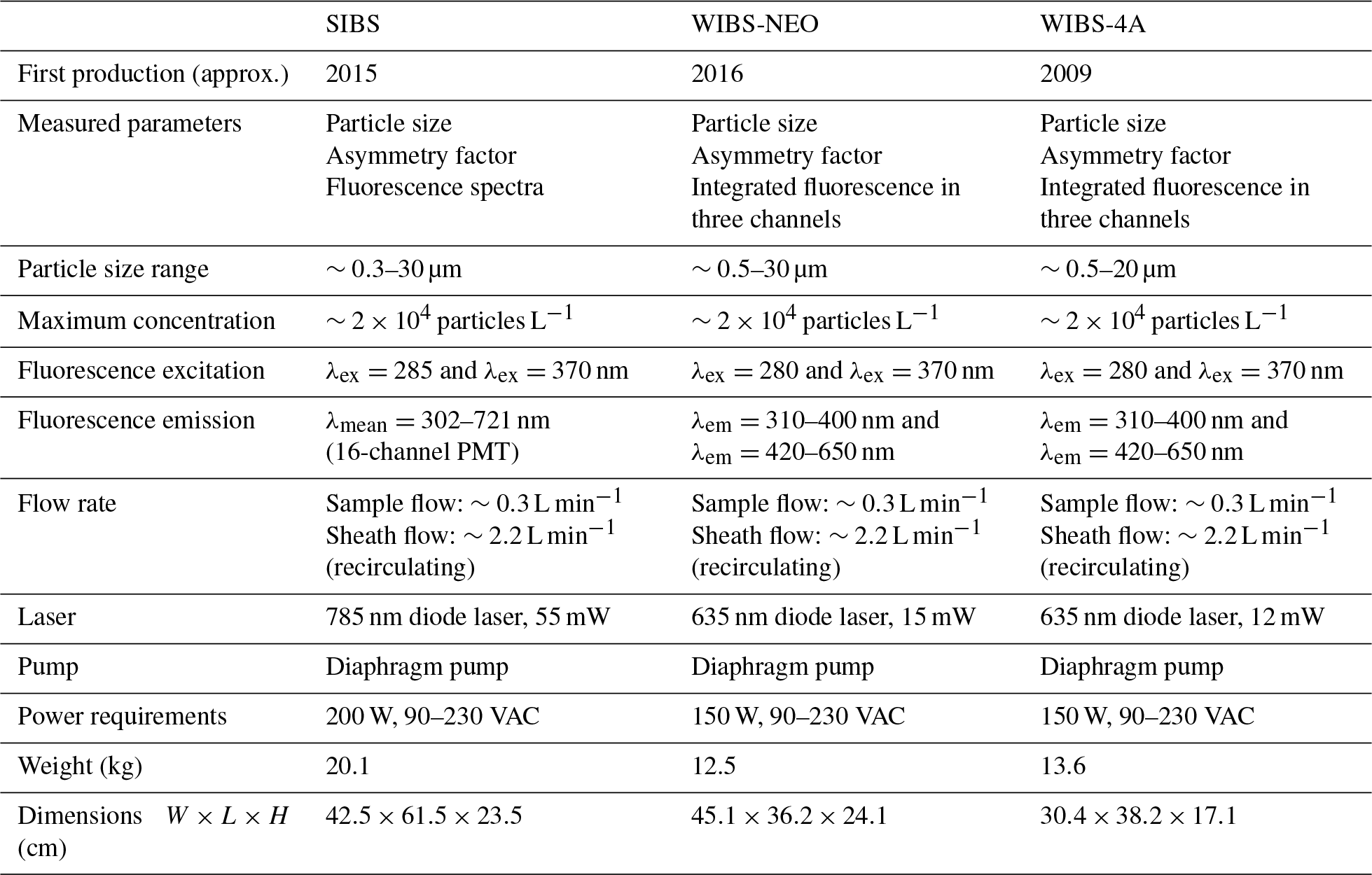
Table 2Parameters and technical components of the SIBS in comparison to the WIBS-NEO and WIBS-4A. Data are taken from manufacturer information.
For the halogen projector lamp, averaged intensity values in each spectral bin were acquired at each power level (150, 200, and 250 W). Spectra measured at 100 W were discarded due to low and unstable emission at wavelengths shorter than ∼500 nm (Fig. S1). Reference spectra and spectra recorded by the SIBS were normalized onto the SIBS detection channel 9 (λmean=528.0 nm), which is theoretically the detection channel with the highest responsivity (see Sect. 4.3). The individual spectral correction factors were calculated by dividing the reference spectra by the spectra derived from the SIBS. The final correction factors are a combination of both light sources whereby the detection channels 1–5 (λmean=302.2–415.6 nm) include the correction factors for the DH-Mini and the detection channels 6–16 (λmean=443.8–721.1 nm) the correction factors for the halogen projector lamp. At the intersection between channel 5 and 6, both corrections (DH-Mini, halogen) are in good agreement. For all particle measurements described in the following sections, the background signal and raw sample spectra recorded by the SIBS were multiplied by those correction factors.
2.5 Microscopy of selected reference particles
Bright field microscopy was conducted using an Eclipse Ti2 (Nikon, Tokyo, Japan) with a 60 × immersion oil objective lens and an additional optical zoom factor of 1.5, resulting in a 90 × magnification. Glass coverslips, used as collection substrates in the particle impactor (Sect. 2.2), were put onto a specimen holder and fixed with tape. Images were recorded using a DS Qi2 monochrome microscope camera with 16.25 megapixels, and Z stacks of related images were created using the software NIS-Elements AR (both Nikon).
2.6 Ambient measurement setup and data analysis
The SIBS was operated between 5 April and 7 May 2018 from a fourth-floor roof laboratory at the Max Planck Institute for Chemistry in Mainz, Germany (49∘59′28.2′′ N, 8∘13′44.5′′ E), similar to measurements as described in Huffman et al. (2010) using a UV-APS. The period between 12 and 18 April 2018 is described here to highlight the capability of the SIBS to monitor ambient aerosol. Beside the SIBS, four additional instruments (data not shown within this study) were connected with ∼20 cm conductive tubing (1∕4 inch) to a sample airflow splitter (Grimm Aerosol Technik GmbH & Co. KG, Ainring, Germany). The splitter was connected to 1.5 m conductive tubing (5∕8 inch), bent out of the window, and connected to 2.4 m stainless-steel tubing (5∕8 inch; Dockweiler AG, Neustadt-Glewe, Germany) vertically installed. Between a TSP head (total suspended particle, custom-made) and the stainless-steel tubing, a diffusion dryer (1 m, 1 kg silica) was installed. Silica was exchanged every third to fourth day and periodic forced trigger measurements were performed daily. The total flow was ∼8.4 L min−1.
For the measurements presented here, particles were only included if they showed fluorescence emission in at least two consecutive spectral channels. This filter was applied to limit noise introduced from measurement artifacts from a variety of sources and will need to be investigated in more detail. The conservative analysis approach here suggests that the values reported are likely to be a lower limit for fluorescent particle number and fraction. However, the observations are in line with previous measurements, providing general support for the fact that the SIBS measurements are reasonable. Note that the maximum repetition rate of the xenon lamps is 125 Hz, corresponding to maximum concentrations of 20 particles per cm3 (see Sect. 3.3). Because ∼50 % of the total coarse particle number was excited by xenon 1 and xenon 2, the fluorescent particle concentrations and fluorescent fractions are corrected accordingly.
The SIBS is based on the general optical design of the WIBS-4A (e.g., Foot et al., 2008; Healy et al., 2012; Hernandez et al., 2016; Kaye et al., 2005; Perring et al., 2015; Robinson et al., 2017; Savage et al., 2017; Stanley et al., 2011) with improvements based on a lower particle sizing limit, resolved fluorescence detection, and a broader emission range. The instrument provides information about size, particle asymmetry, and fluorescence properties for individual particles in real time. The excitation wavelengths are optimized for the detection of the biological fluorophores tryptophan, NAD(P)H, and riboflavin. However, other fluorophores in PBAPs will certainly fluoresce at these excitation wavelengths as many of them cluster in two spectral fluorescence “hotspots” as summarized in Pöhlker et al. (2012 and references therein) and as shown for WIBS-4A measurements by Savage et al. (2017). Figure 1 shows an overview of excitation wavelengths and emission ranges of the UV-APS, WIBS-4A, WIBS-NEO, and SIBS for bioaerosol detection in relation to the spectral location of selected biofluorophores, such as tyrosine, tryptophan, NAD(P)H, riboflavin, and chlorophyll b. At λex=285 nm, the SIBS excites fluorophores in the “protein hotspot” and at λex=370 nm fluorophores in the “flavin–coenzyme hotspot” (Pöhlker et al., 2012). In contrast to the UV-APS, the SIBS is able to detect fluorescence signals from chlorophyll due to the extended upper spectral range of detection (up to λem=721 nm). Both the WIBS-4A and WIBS-NEO cover the spectral emission range for chlorophyll b, but cannot provide resolved spectral information to separate it from other fluorophores. Table 2 summarizes and compares the parameters and technical components of the SIBS, WIBS-4A, and WIBS-NEO. The individual components are described in detail in the subsequent sections.
To avoid potential misunderstanding, it is important to note that the SIBS described in this study is not related to spark-induced breakdown spectroscopy instrumentation, which uses the same acronym (e.g., Bauer and Sonnenfroh, 2009; Hunter et al., 2000; Khalaji et al., 2012; Schmidt and Bauer, 2010). The DMT SIBS discussed here was recently used as part of a test chamber study (Nasir et al., 2018), but the study here is the first to discuss important technical details of the instrument design and operation.
3.1 Aerosol inlet and flow diagram
The design for the aerosol inlet of the SIBS is identical to the inlet of the WIBS-4A and WIBS-NEO. A detailed flow diagram is shown in Fig. 2a. Aerosol is drawn in via an internal pump as laminar airflow through a tapered delivery nozzle (Fig. 2a.1) with which sheath (∼2.2 L min−1) and sample flow (∼0.3 L min−1) are separated.
3.2 Size and shape analysis
After passing the delivery nozzle, entrained particles traverse a 55 mW continuous-wave diode laser at λ=785 nm (position no. 1 in Fig. 2b and no. 2 in Fig. S2). Unlike in the WIBS-4A and WIBS-NEO (635 nm diode laser), the triggering laser in the SIBS is in the near-infrared (IR) region (>700 nm) and therefore outside the detectable emission range of the 16-channel photomultiplier tube (PMT) to avoid scattered light from the particle trigger laser being detected (see Fig. 1). The side- and forward-scattered light is collected and used for subsequent measurements. Side-scattered light is collected by two concave mirrors, which are directed at 90∘ from the laser beam axis and reflect the collected light onto a dichroic beam splitter (no. 7 in Fig. S2). A PMT (H10720-20; Hamamatsu Photonics K.K., Japan) converts incoming light signals into electrical pulses, which are used for particle triggering and sizing (no. 6 in Fig. S2). For the determination of the optical particle size, the SIBS uses a calculated calibration curve according to Lorenz–Mie theory, assuming spherical and monodisperse PSLs with a refractive index of 1.59 (Brandrup et al., 1989; Lorenz, 1890; Mie, 1908). Compared to aerodynamic sizing, which depends on particle morphology and density (e.g., Reid et al., 2003; Reponen et al., 2001), the calculated optical diameter can vary significantly if the assumption of sphericity is not fulfilled. In contrast, optical sizing is not as affected by differences in material density. The instrument operator must thus be aware of uncertainties in measured particle size due to, e.g., particle morphology and the spatial orientation of a particle when traversing the trigger laser or changing refractive indices. In contrast to the WIBS-4A, the SIBS and WIBS-NEO detect the full range of particle sizes (SIBS: ∼0.3 and 30 µm (nominal); WIBS-NEO: ∼0.5 and 30 µm, nominal) by using one PMT gain setting instead of switching between a “low gain” and “high gain” setting. The physical and technical details of this gain-switching method are patent pending and are not publicly available.

Figure 2SIBS flow diagram in (a): (1) tapered delivery nozzle. (2) Intersection of sample flow and laser beam. Sampling volume: ∼0.7 mm diameter; ∼130 µm of depth. (3) Filtered (through HEPA filter) and recirculating sheath flow. (4) Needle valve for adjusting purge flow, which constantly purges the optical cavity. SIBS measurement cycle in (b); position 1: particles scatter light in all directions after being illuminated by a diode laser (λ=785 nm). Position 2: xenon lamp 1 is firing at λex=285 nm. Position 3: xenon lamp 2 is firing at λex=370 nm. The measurement cycle from position 1 to position 3 takes ∼25 µs over a distance of ∼300 µm. (a) Modified; image courtesy of DMT. Panel (b) adapted from WIBS-4A service manual (DOC-0345 rev. A; DMT, 2012).
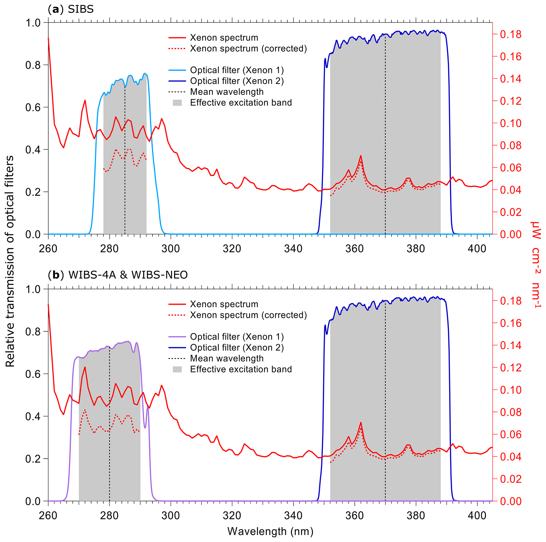
Figure 3Irradiance from xenon flash lamps based on the specifications of lamps and optical filters. Purple and blue lines show the optical transmission of filters (left axes) applied to select excitation wavelength. Gray bands indicate where filters transmit light relative to the mean wavelength. Red lines show theoretical irradiance values of the xenon flash lamp (right axes): solid line (raw output), dashed line (relative output after filtering). Relative output is shown as raw output multiplied by the effective excitation band of the bandpass filters used in the (a) SIBS (Δλex (Xe1) = ∼14 nm; Δλex (Xe2) = ∼36 nm) and (b) WIBS-4A and WIBS-NEO (Δλex (Xe1) = ∼20 nm; Δλex (Xe2) = ∼36 nm). Xenon lamp operating conditions: 600 V main voltage, 0.22 µF main capacitance, 126 Hz repetition rate, 500 mm distance. (Data courtesy of Xenon flash lamps, Hamamatsu; single-band bandpass filters, Semrock.)
The forward-scattered light is measured by a quadrant PMT (no. 5 in Fig. S2) to detect the scatter asymmetry for each particle (Kaye et al., 1991, 1996). A OG-515 long-pass filter (Schott AG, Mainz, Germany) prevents incoming light from the xenon flash lamps in a spectral range below 515±6 nm from reaching the quadrant PMT. To calculate the AF, the root mean square variations for each quadrant of the PMT of the forward-scattered light intensities are used (Gabey et al., 2010). The AF broadly relates whether a particle is more spherical or fibril. Theoretically, for a perfectly spherical particle, the AF would be 0, whereas an elongated particle would correspond to an AF of 100 (Kaye et al., 1991). However, due to electrical and optical noise from the quadrant PMT, the AF value of a sphere is usually between ca. 2 and 6 (according to WIBS-4A service manual, DOC-0345 rev. A). Because the AF value depends on the physical properties of optical components, the baseline for spherical particles may shift even within identical instruments (Savage et al., 2017). For example, the study by Toprak and Schnaiter (2013) reported an average AF value for spherical particles of 8 using a WIBS-4A. In contrast, AF values shown by Foot et al. (2008) were, on average, below ∼5 for spherical particles measured with a WIBS-2s prototype.
3.3 Fluorescence excitation
Two xenon flash lamps (L9455-41; Hamamatsu) (no. 3 and no. 4 in Fig. S2) are used to induce fluorescence. They emit light pulses, which exhibit a broad excitation wavelength range of 185 to 2000 nm. The light is optically filtered to obtain a relatively monochromatic excitation wavelength. Further information about the spectral properties of the xenon flash lamps can be found elsewhere (specification sheet TLSZ1006E04, Hamamatsu, May 2015). Figure 3 displays relevant optical properties of the lamps and filters used within the SIBS, WIBS-4A, and WIBS-NEO. For the SIBS, a BrightLine® FF01-285/14-25 (Semrock Inc., Rochester, NY, USA) single-band bandpass filter is used with λmean=285 nm and an effective excitation band2 of 14 nm width is used for xenon 1. For xenon 2, the single-band bandpass filter BrightLine® FF01-370/36-25 (Semrock) is used with λmean=370 nm and with an effective excitation band of 36 nm width. The only difference among all three instruments is that the WIBS-4A and WIBS-NEO use a different single-band bandpass filter for xenon 1 (Semrock, BrightLine® FF01-280/20-25; λmean=280 nm; effective excitation band of 20 nm). The excitation light beam for all three instruments is focused on the sample flow within the optical cavity, resulting in a rectangular beam shape of ∼ 5 mm by 2 mm. Xenon 1 is triggered when particles pass position 2 in Fig. 2b, and approximately 10 µs later xenon 2 is triggered as the particles move further to position 3 in Fig. 2b. After firing, the flash lamps need ∼5 ms to recharge. During the recharge period, particles are counted and sized but no fluorescence information is recorded. The maximum repetition rate of the xenon lamps yields a measurable particle number concentration of L−1 (corresponding to 20 cm−3).
Irradiance values from light sources become a crucial factor when interpreting derived fluorescence data from LIF instruments because the fluorescence intensity (F) is directly proportional to the intensity of incident radiant power, described by the relationship
Φ: quantum efficiency, I0: intensity of incident light, ε: molar absorptivity, b: path length (cell), c: molar concentration (Guilbault, 1990).
To measure the irradiance of each xenon lamp after optical filtering, we used a thermal power head (S425C; Thorlabs), which was placed at a distance of 11.3 cm (focus length from xenon arc bow to sample flow intersection) from the xenon lamp measuring over a duration of 1 min at 10 xenon shots per second. By measuring new xenon lamps, we observed an average irradiance of 14.8 mW cm−2 for xenon 1 and 9.6 mW cm−2 for xenon 2, corresponding to ∼154 % higher irradiance (spectrally integrated) from xenon 1. A second set of lamps used intermittently for 3 years, including several months of continuous ambient measurements and a lab study with high particle concentrations, exhibited average irradiance values of 10.8 mW cm−2 (1σ SD 1.8 mW cm−2) for xenon 1 and 4.9 mW cm−2 (1σ SD 1.9 mW cm−2) for xenon 2, corresponding to ∼220 % higher irradiance from xenon 1. Comparing the nominal, transmission-corrected irradiance data from the two xenon lamps provided by the lamp supplier (Fig. 3a and b, red dashed lines), an irradiance imbalance between xenon 1 and xenon 2 can be assumed for all three LIF instruments discussed here (SIBS, WIBS-4A, and WIBS-NEO).
The results shown here are comparable to multiple WIBS studies (e.g., Hernandez et al., 2016; Perring et al., 2015; Savage et al., 2017), in which fluorescence emission intensities at λex=280 nm (xenon 1) also show a tendency to be higher than those at λex=370 nm (xenon 2).
3.4 Spectrally resolved fluorescence detection
Fluorescence emission from excited particles is collected by two parabolic mirrors in the optical cavity and delivered onto a custom-made dichroic beam splitter (Semrock, no. 7 in Fig. S2). The beam splitter allows for the transmission of incoming light between ∼300 and 710 nm, with an average transmission efficiency of 96 %. At wavelengths shorter than 300 nm, the transmission decreases rapidly to <20 % at 275 nm. At the upper detection end of the SIBS (λmean=721 nm), the transmission efficiency decreases to ∼89 %. The scattering light from the diode laser is reflected at a 90∘ angle onto the PMT used for particle detection and sizing. At the excitation wavelength of 785 nm, the reflection efficiency is stated at ∼95 % (Fig. S3).
After passing the dichroic beam splitter, the photons are led into a grating polychromator (A 10766; Hamamatsu) (no. 8 in Fig. S2). A custom-made transmission grating (Hamamatsu) is used to diffract incoming light within a nominal spectral range between 290.8 and 732.0 nm. In the case of the SIBS, a grating with 300 g mm−1 groove density and 400 nm blaze wavelength is used, resulting in a nominal spectral width of 441.2 nm and a resolution of 28.03 nm mm−1. After passing the transmission grating, the diffracted light hits a 16-channel linear array multi-anode PMT (H12310-40; Hamamatsu) (no. 9 in Fig. S2) with defined mean wavelengths for each channel as shown in Table 1.
For each single particle detected, two spectra are recorded at λex=285 and 370 nm. The detectable band range of the PMT overlaps the excitation wavelength of xenon 2. Therefore, a notch optical filter (Semrock) is placed between the optical chamber and the grating polychromator to prevent the detector from being saturated. Incoming light at wavelengths shorter than 300 nm and from 362 to 377 nm is blocked from reaching the PMT, resulting in a reduced spectral bin width for detection channels 1, 3, and 4. The first three detection channels are omitted because their mean wavelengths are below λex=370 nm (see also Fig. 1). Accordingly, the emission spectra for xenon 2 excitation begin at channel 4 (λmean=387.3 nm).
Technical data (xenon flash lamps, filters, dichroic beam splitter, PMT responsivity, and transmission grating) described in the previous sections (Sect. 3.3 and 3.4) were provided by Hamamatsu and Semrock. Note that the transmission–reflection efficiencies of the dichroic beam splitter, the cathode radiant sensitivity of the PMT, and diffraction efficiency data are modeled. Thus, individual components may differ slightly from modeled values, even within the same production batch. Neither company assumes data accuracy or provides warranty, either expressed or implied.
The SIBS was originally designed and marketed to record time-resolved and spectrally resolved fluorescence lifetimes at two excitation wavelengths. The fluorescence lifetimes of most biofluorophores, serving as targets for bioaerosol detection, are usually below 10 ns (e.g., Chorvat and Chorvatova, 2009; Herbrich, et al., 2012; O'Connor et al., 2014; Richards-Kortum and Sevick-Muraca, 1996). However, by choosing xenon lamps as an excitation source, recording the relevant fluorescence lifetimes in this nanosecond range is hampered by the relatively long decay time of the xenon lamp excitation pulse (∼1.5 µs). In principle, fluorescence lifetime measurements would be possible if the xenon lamps were replaced by appropriate laser excitation sources in the SIBS optical design.
3.5 Software components and data output
The SIBS uses an internal computer (no. 10 in Fig. S2) with embedded LabVIEW-based data acquisition software allowing the user to control functions in real time and change multiple measurement parameters. As an example, the “single particle” tab from the SIBS interface is shown in Fig. S4. Here, the user can define, e.g., the sizing limits of the SIBS (upper and lower threshold) and the minimum size of a particle being excited by the xenon flash lamps. Furthermore, forced trigger measurements can be performed while on this particular tab. Subsequently, the term “forced trigger measurement” will be replaced by “background signal measurement”. A local Wi-Fi network is installed so that the SIBS can be monitored and controlled remotely. A removable hard drive is used for data storage. Data are stored in HDF5 format to minimize storage space and optimize data write speed. The resulting raw data are processed in Igor Pro. As an example, by using a minimum sizing threshold of 500 nm, the SIBS data output per day, operating in a relatively clean environment (∼40 particles per cm−3), can span several hundred MB. In contrast, the data output can increase up to ∼3 GB daily in polluted areas (∼680 particles per cm−3). By lowering the minimum sizing threshold to 300 nm, the data volume can exceed 10 GB per day when sampling in a moderately polluted environment (∼180 particles per cm−3).

Figure 4Size calibration of SIBS. Black horizontal bars indicate 1σ SD as stated by each manufacturer (Table S1). Optical diameter values and related 1σ SD are based on a Gaussian fit, which was used to average size distributions of several thousand homogeneous particles for each measurement. The linear fit (red dashed line) excludes the 0.356 µm PSL sample (red marker), an outlier potentially caused by a poor-quality PSL batch. Only nonfluorescent particle standards were used for determining the sizing accuracy.
4.1 Validation of SIBS sizing
To validate the optical sizing of the SIBS, 20 particle size standards were analyzed, covering a broad size range from 0.3 to 20 µm in particle diameter. Overall, the particle size measurements from the SIBS (optical diameter) show good agreement with the corresponding measurements of physical diameter reported by PSL and PS-DVB manufacturers (Fig. 4). For the SIBS, the manufacturer states a nominal minimum size detection threshold of 0.3 µm. Figure 4 shows that a linear response between optical particle size and physical particle size extends down to at least 0.3 µm. Smaller particles were not investigated. The upper size detection threshold is reported by the manufacturer to be nominally 30 µm. However, the upper limit was not investigated here due to the difficulty in aerosolizing particles larger than 20 µm. In most field applications, the upper particle size cut is often far below this value due to unavoidable sedimentation losses of large particles in the inlet system (e.g., Moran-Zuloaga et al., 2018; Von der Weiden et al., 2009). Note that the size distributions of physical diameter for PS-DVB standards are broader compared to the PSL standards, as reported by the manufacturer (Table S1). This also translates to broader distributions of optical diameter measured by the SIBS for PS-DVB than for PSL particles. The 0.356 µm PSL sample was an outlier with respect to the overall trend, showing an optical diameter of 0.54 µm. We suspect that this deviation between physical and optical size can be explained by the poor quality of this particular PSL sample lot rather than an instrumental issue, so it was not included in the calculation of the trend line (Fig. 4). Furthermore, the SIBS was shown to slightly undersize the PSLs between 0.6 and 0.8 µm; however, the overall trend exhibits a coefficient of determination of r2>0.998.
As mentioned in Sect. 3.2, an important point regarding the SIBS and WIBS-NEO is that the size calibration within the unit cannot be changed by the user, meaning that the PMT output voltages are transformed directly to outputted physical diameter within the internal computer using a proprietary calculation. It is still important, however, for the user to perform sizing calibration checks frequently to verify and potentially post-correct the particle sizing of all particle sizing instruments, including the SIBS and WIBS-NEO.
4.2 Amplification of fluorescence detector
As with all optical detection techniques, an adequate understanding of detection thresholds is an essential aspect of instrument characterization and use (e.g., Jeys et al., 2007; Savage et al., 2017). The application of appropriate voltage gain settings must be applied to the physical detection process so as not to lose information about particles that cannot be recovered by post-processing data. Yet particles in the natural atmosphere exhibit an extremely broad range of fluorescence intensities (many orders of magnitude), arising from the breadth of quantum yields for fluorophores occurring in aerosols and from the steep increase in fluorescence emission intensity with particle size (second to third power) (e.g., Hill et al., 2015; Könemann et al., 2018; Sivaprakasam et al., 2011; Swanson and Huffman, 2018). This range of fluorescence properties is generally broader than the dynamic range of any single instrument, so a UV-LIF instrument can be operated, e.g., to either (i) apply a higher detector gain to allow for high sensitivity toward detecting weakly fluorescing particles, often from rather small particles (<1 µm), at the risk of losing fluorescence information for large or strongly fluorescent particles due to detector saturation, or (ii) apply a lower detector gain to preferentially detect a wide range of more highly fluorescent particles, but at the risk of not detecting weakly fluorescent or small particles.
The amplification voltage of the 16-channel PMT used in the SIBS can be adjusted between 500 and 1200 V. Each of the 16 detection channels can also be individually adjusted using digital gain settings within the SIBS acquisition software. This channel-specific gain does not affect the amplification process (e.g., the dynode cascade), but rather modifies the output signal of a single detection channel digitally. The digital gain is applied only after the signal collection process and therefore cannot compensate for a signal that is below the noise threshold or that saturates the detector. The digital gain was thus left at the maximum gain level (255 arbitrary units, a.u.) for all channels during particle measurements discussed here.
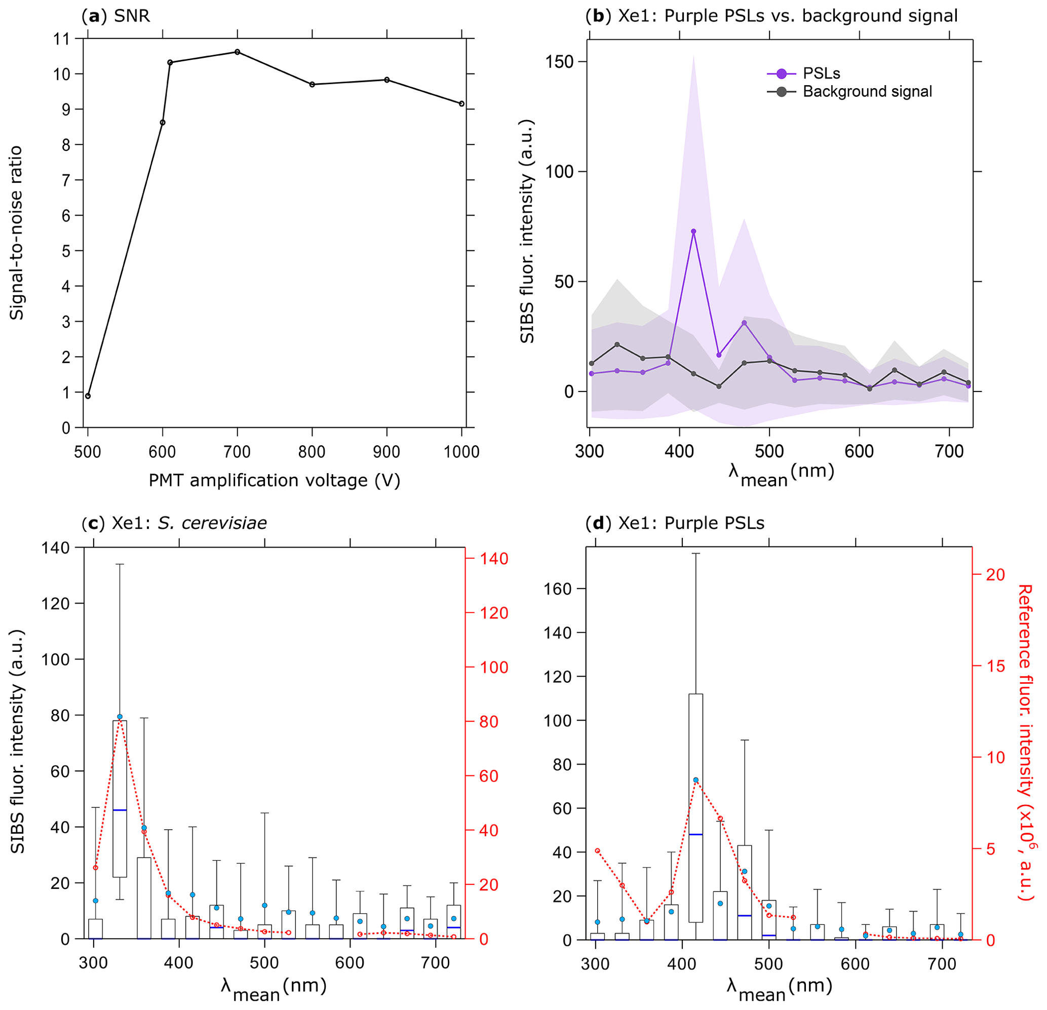
Figure 5SIBS signal-to-noise ratio (SNR); (a) emission of 0.53 µm purple PSLs (5260 particles, background signal + 1σ SD subtraction) divided by background signal at different PMT amplification voltages (both at Xe1, channel 5, averaged and uncorrected). Background signal measured over 5 min. (b) Fluorescence emission in contrast to background signal at a PMT amplification voltage of 610 V (same parameters as in a). Shaded area: 1σ SD. Fluorescence intensity values are shown in arbitrary units. Fluorescence emission spectra of (c) S. cerevisiae (yeast; 2048 particles, 0.5–1 µm) and (d) PSLs (as in b). Red dashed lines and markers (right axes) show averaged and re-binned reference spectra. Box and whisker plots (left axes) show SIBS spectra: median (blue line), mean (circle); boxes 75th and 25th percentile, whiskers 90th and 10th percentile. Data coinciding with first- or second-order elastic scattering were removed from reference spectra.
To explore the influence of amplification voltage on particle detectability, 0.53 µm purple PSLs were chosen to arbitrarily represent the lower limit of detectable fluorescence intensity. Using larger (0.96 µm) particles comprised of the same purple fluorophore, Könemann et al. (2018) showed that the particles were only narrowly detectable above the fluorescence threshold in each of the three channels of a WIBS-4A (same unit as used in Savage et al., 2017), so the smaller 0.53 µm PSLs were chosen here as a first proxy for the most weakly fluorescing particles we would expect to detect. To improve the signal-to-noise ratio (SNR) for the lower fluorescence detection limit, the PMT amplification voltage was varied in seven steps between 500 and 1000 V (corresponding to a gain from 103 to 106; specification sheet TPMO1060E02, Hamamatsu, June 2016) for purple PSLs and background signals (Fig. 5a). Whereas PSL spectra at a PMT amplification of 500 V were indistinguishable from the background signal (+1σ SD), spectra show a discernable peak at λmean=415.6 nm above 600 V. Subsequently, the SIBS was operated with a PMT amplification voltage of 610 V corresponding to the lowest SNR threshold accepted (Fig. 5a, b). The detection of small biological particles was tested by measuring the emission spectrum of S. cerevisiae as an example of a PBAP (see also Pöhlker et al., 2012). On average, the size of intact S. cerevisiae particles ranges from ∼2–10 µm (e.g., Pelling et al., 2004; Shaw et al., 1997). To test the ability of the SIBS to detect low-intensity emissions, we separately analyzed S. cerevisiae particles between 0.5 and 1 µm, which most likely includes cell fragments caused by the aerosolization process (Fig. 5c). The tryptophan-like emission, peaking in detection channel 2 (λmean=330.6 nm) for λex=285 nm, reveals intensity values below 100 a.u., which are comparable to fluorescence intensity values derived from 0.53 µm purple PSLs (detection channel 5, λmean=415.6 nm; Fig. 5d). These two tests for S. cerevisiae and 0.53 µm purple PSLs confirmed the instrument ability to detect emission spectra from particles at least as strongly fluorescent as these two test cases, leaving a wide range to detect larger and more intensely fluorescing particles. By using a 3σ SD threshold, the fluorescence peak at λmean=415.6 nm of 0.53 µm purple PSLs is still detectable but can no longer be distinguished from the background signal at a 6σ SD threshold. Therefore, fluorescence intensity values at the lower detection limit should be treated with care. Corrected spectra of both S. cerevisiae and 0.53 µm purple PSLs can be found in the Supplement (Fig. S5). By operating the SIBS at a relatively low detector amplification, very weak fluorescence, especially from small particles (<1 µm), might not exceed the detection threshold during field applications and would be missed. Further investigation will be necessary to choose amplification voltages appropriate for individual applications in which smaller or otherwise weakly fluorescent particles might be particularly important. For all subsequent measurements discussed here, a PMT amplification voltage of 610 V was used.
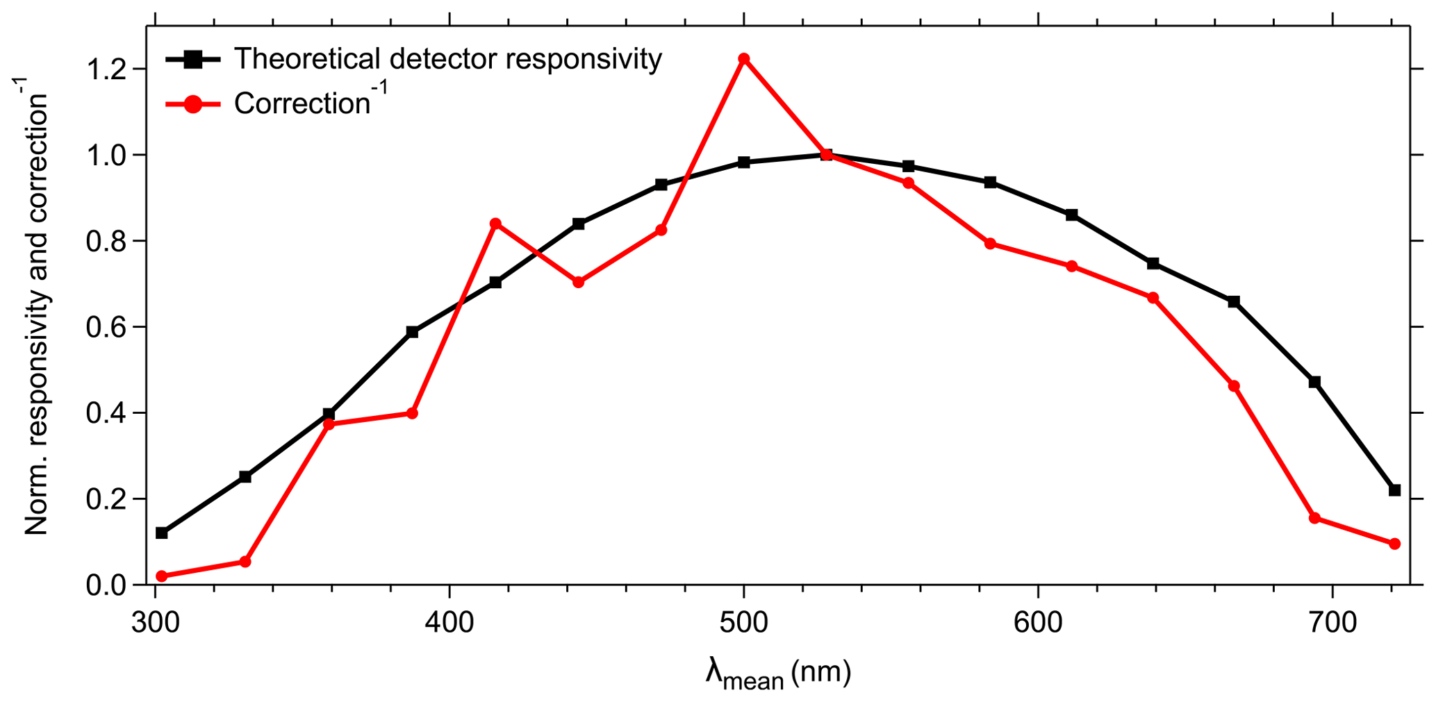
Figure 6Normalized theoretical detector responsivity and spectral correction. Theoretical detector responsivity derived from measured cathode radiant sensitivity multiplied by the diffraction efficiency (as shown in Fig. S7). Note that the red line shows the inverse of spectral correction to match detector response.
Saturation only occurred for 15 and 20 µm nonfluorescent PS-DVB particles. As highlighted in Fig. S6, the polystyrene–detergent signal (Könemann et al., 2018) at λex=285 nm for 10 µm PS-DVB particles can be spectrally resolved (Fig. S6b), whereas the spectrum for 15 µm PS-DVB particles (Fig. S6e) is altered due to single particles (∼10 % out of 400 particles) saturating the detector (at 62 383 a.u.). By comparing the defined lower detection end (Fig. 5) to the upper end (Fig. S6), a quantitative difference of approximately 3 orders of magnitude can be estimated, indicating a wide detectable range at the chosen amplification voltage setting.
4.3 Wavelength-dependent spectral correction of detector
The 16 cathodes of the PMT should be considered as independent detectors with wavelength-dependent individual responsivity and amplification characteristics. In combination with the physical properties of technical components (e.g., excitation sources, optical filters, gratings), an instrumental-specific spectral bias might result in incorrect or misleading spectral patterns if not corrected (e.g., DeRose, 2007; DeRose et al., 2007; Holbrook et al., 2006). To compensate for such potential instrumental biases, we used a spectral correction approach as described in Sect. 2.4. The spectral correction factors are comparable to the theoretical responsivity of the PMT with the highest correction for channels 1–4 (λmean=302.2–387.3 nm) and 14–16 (λmean=666.5–721.1 nm) (Fig. 6). Channel 8 (λmean=500.0 nm) shows the highest responsivity and channels 6 and 7 (λmean=443.8 and 471.9 nm) exhibit a noticeable lower responsivity than their adjacent channels (see also Sect. 4.4.1). The spectral correction shows several peaks (e.g., detector channels 3, 5, and 8) and dips (e.g., detector channels 4, 6, and 7) (Fig. 6); however, this pattern is due to gain variations for different channels and is not noise.
It is important to note that the detector settings and spectral correction uniquely refer to the SIBS unit as it was used for the current study. Due to technical and physical variability as stated above, it is likely that the spectral correction required for other SIBS units would be somewhat different. Furthermore, the wavelength-dependent detector correction may change over time due to material fatigue or contamination in the optical chamber affecting background signal measurements. Periodic surveillance and adjustments are therefore required, especially after measurements for which the instrument was exposed to high particle concentrations or was operated during extreme weather or environmental conditions (e.g., temperature, humidity, vibration). For particle sizing verification, we recommend the use of 0.5, 1, and 3 µm nonfluorescent PSLs. Regarding a fluorescence response check, we recommend 2 µm green and 2 µm red PSLs for the validation of the spectral responsivity maximum and the upper (near-IR) detection range. To our knowledge, no fluorescent dyed PSLs are available to verify the response within the lower spectral detection range (UV) of the SIBS. However, the polystyrene signal of 3 µm nonfluorescent PSLs (Fig. S6g, h, i; see also Könemann et al., 2018) represents a compromise between signal strength at λex=285 nm and aerosolization efficiency (compared to PSLs with larger sizes) for a spectral responsivity validation.
4.4 Fluorescence spectra of standards
4.4.1 PSL standards
The SIBS spectra for the four different PSL standards, covering an emission range from UV to near-IR, generally agree well with the corresponding reference spectra (Fig. 7). Each of the two excitation wavelengths probe separate fluorescent modes, which appear at approximately the same emission wavelength for a given PSL type (e.g., nm for red PSLs; Fig. 7j), as discussed by Könemann et al. (2018). Moreover, even the rather weak polystyrene and detergent fluorescence systematically associated with PSL suspensions (Könemann et al., 2018) is resolved by the SIBS at λex=285 nm and λem = ∼300 nm (Fig. 7b, e, h, k). It is further noteworthy that emission intensity at λex=285 nm is generally higher than derived emission intensity at λex=370 nm (Fig. 7c, f, i, l), supporting the finding that a particle receives higher irradiance values from xenon 1 than from xenon 2 (see also Sect. 3.3).
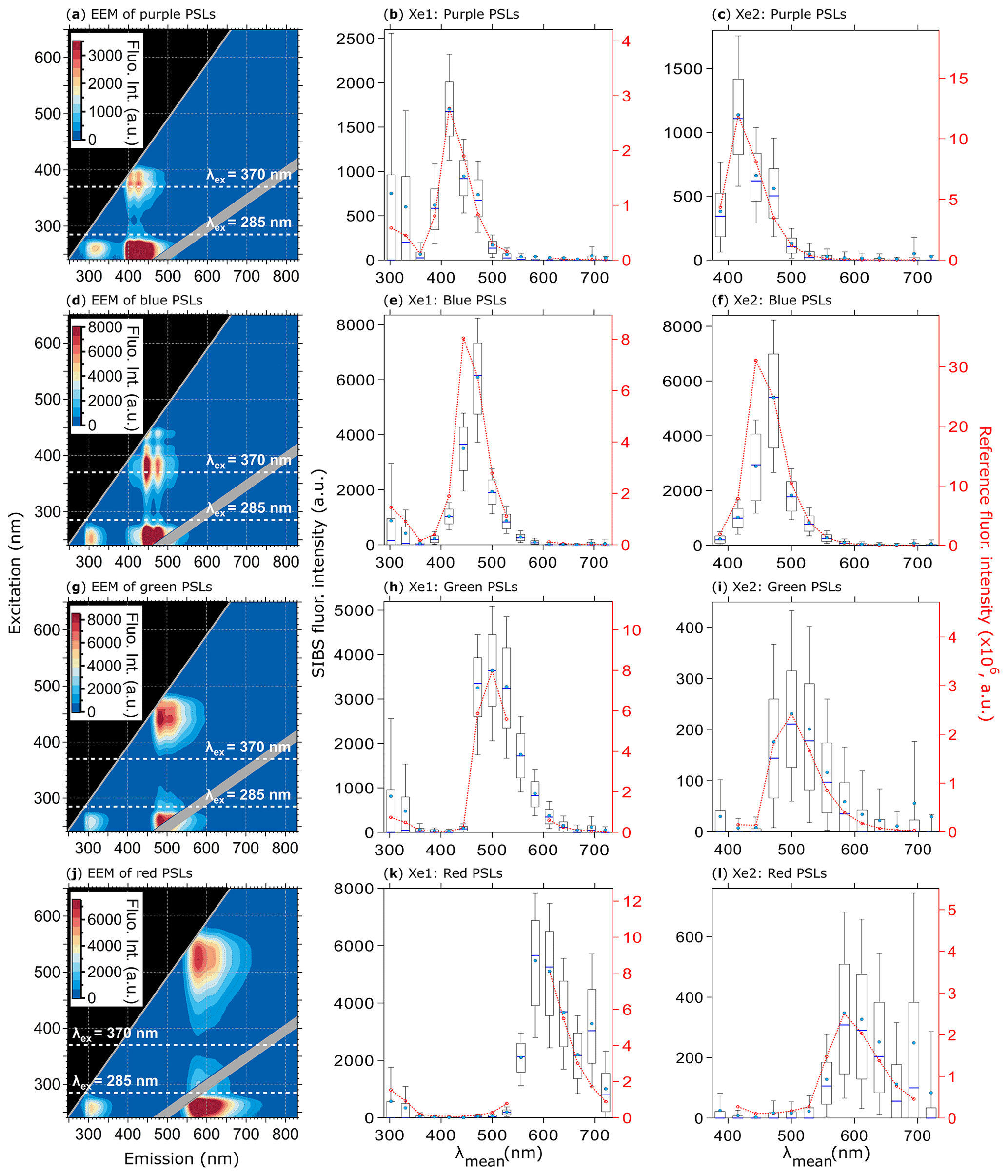
Figure 7Fluorescence emission spectra of PSLs. Steady-state fluorescence signatures displayed as EEMs (left column) and spectra at Xe1 and Xe2 (middle, right columns) for 2.07 µm purple (a, b, c, 1082 particles), 2.1 µm blue (d, e, f, 1557 particles), 2 µm green (g, h, i, 1174 particles), and 2 µm red PSLs (j, k, l, 1474 particles). Within EEMs: white dashed lines show SIBS excitation wavelengths (λex=285 and 370 nm), and gray diagonal lines indicate first- and second-order elastic scattering bands (both bands were subtracted automatically by the Aqualog V3.6 software). Red dashed lines and markers (right axes; middle, right columns) are averaged and re-binned reference spectra. Box and whisker plots (left axes) show SIBS spectra: median (blue line), mean (circle); boxes show the 75th and 25th percentile, and whiskers show the 90th and 10th percentile. Data coinciding with first- or second-order elastic scattering were removed from reference spectra.
As mentioned in Sect. 4.3, detection channels 6 and 7 require relatively large correction factors. For 2.07 µm purple PSLs (Fig. 7b, c), the SIBS spectra closely match the reference spectra after correction. For the 2.1 µm blue PSLs (Fig. 7e, f), however, the corrected spectrum matches the reference spectrum well, except at detection channel 6 (λmean=443.8 nm), in which the SIBS spectrum is lower than the reference spectrum by approximately 50 %. This effect was also observed for 1 µm blue PSLs (Thermo Fisher, B0100) doped with the same fluorophore (data not shown). The reason for this discrepancy is unknown. Nevertheless, because this effect only occurs noticeably for highly fluorescent blue PSLs and NAD (see also Sect. 4.4.2), one explanation could be that the instrument-dependent dynode cascade (the electronic amplification stages) for this particular detection channel is suppressed, resulting in a lower amplification efficiency. In this case, relatively low signals could be amplified correctly, whereas medium- or high-intensity emissions could only be amplified up to a certain level. The amplification threshold for detection channel 6 is, however, unknown and needs further verification.
4.4.2 Biofluorophore standards
Figures 8 and 9 highlight the fluorescence spectra of different biofluorophores measured by the SIBS, which correspond to related reference spectra (compare also Pöhlker et al., 2012), showing that amino acids (fluorescence emission only at λex=285 nm), coenzymes and flavin compounds (fluorescence emission at λex=285 and 370 nm), and chlorophyll (fluorescence emission only at λex=370 nm) can be spectrally distinguished.
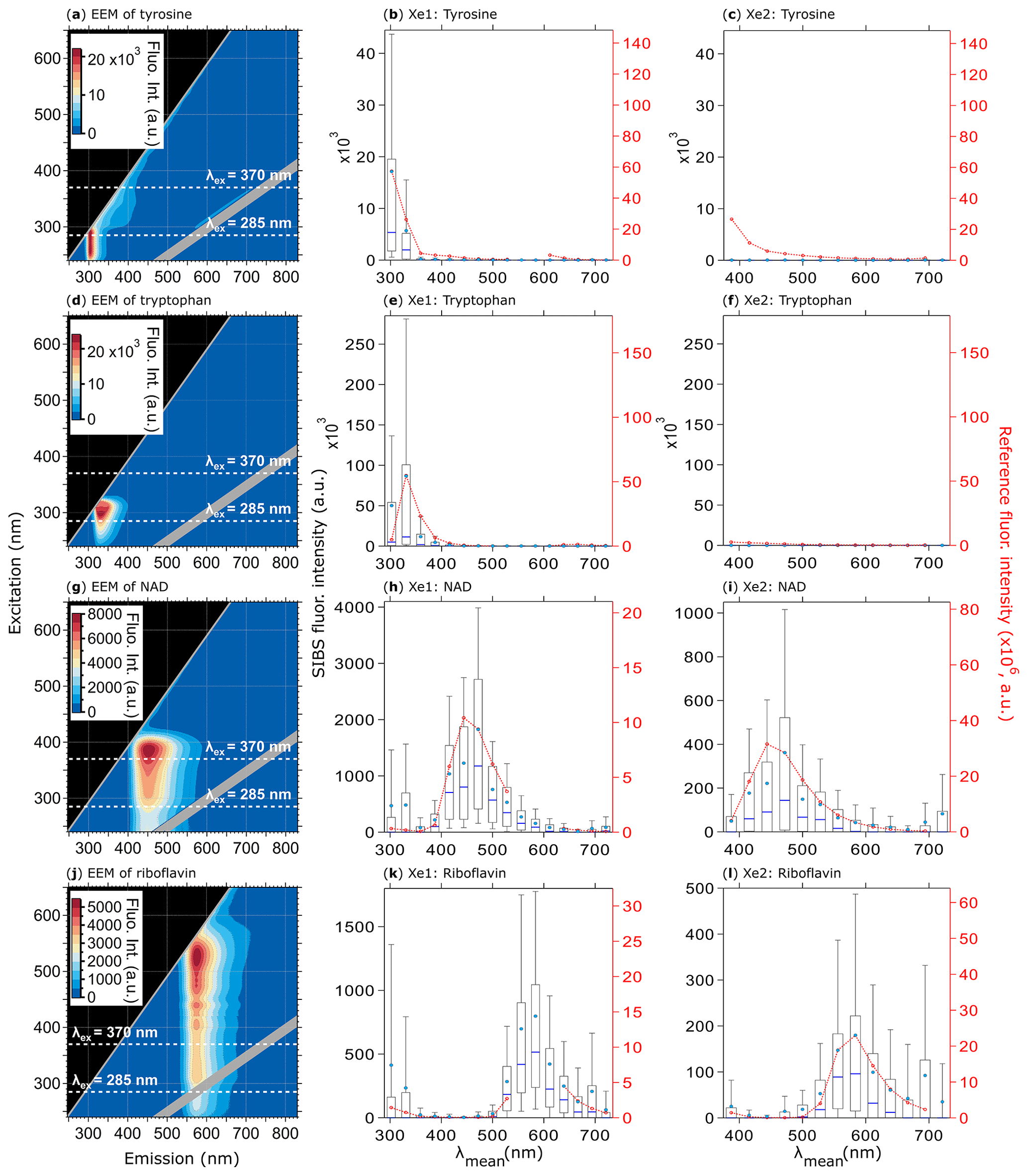
Figure 8Fluorescence emission spectra of biofluorophores. EEMs (left column) and spectra at Xe1 and Xe2 wavelengths (middle and right columns) shown for tyrosine (a, b, c, 209 particles), tryptophan (d, e, f, 193 particles), NAD (g, h, i, 376 particles), and riboflavin (j, k, l, 205 particles). Red dashed lines and markers (right axes; middle, right columns) are averaged and re-binned reference spectra. Box–whisker plots and EEMs as described in Fig. 7. All biofluorophores were size-selected between 1 and 2 µm.
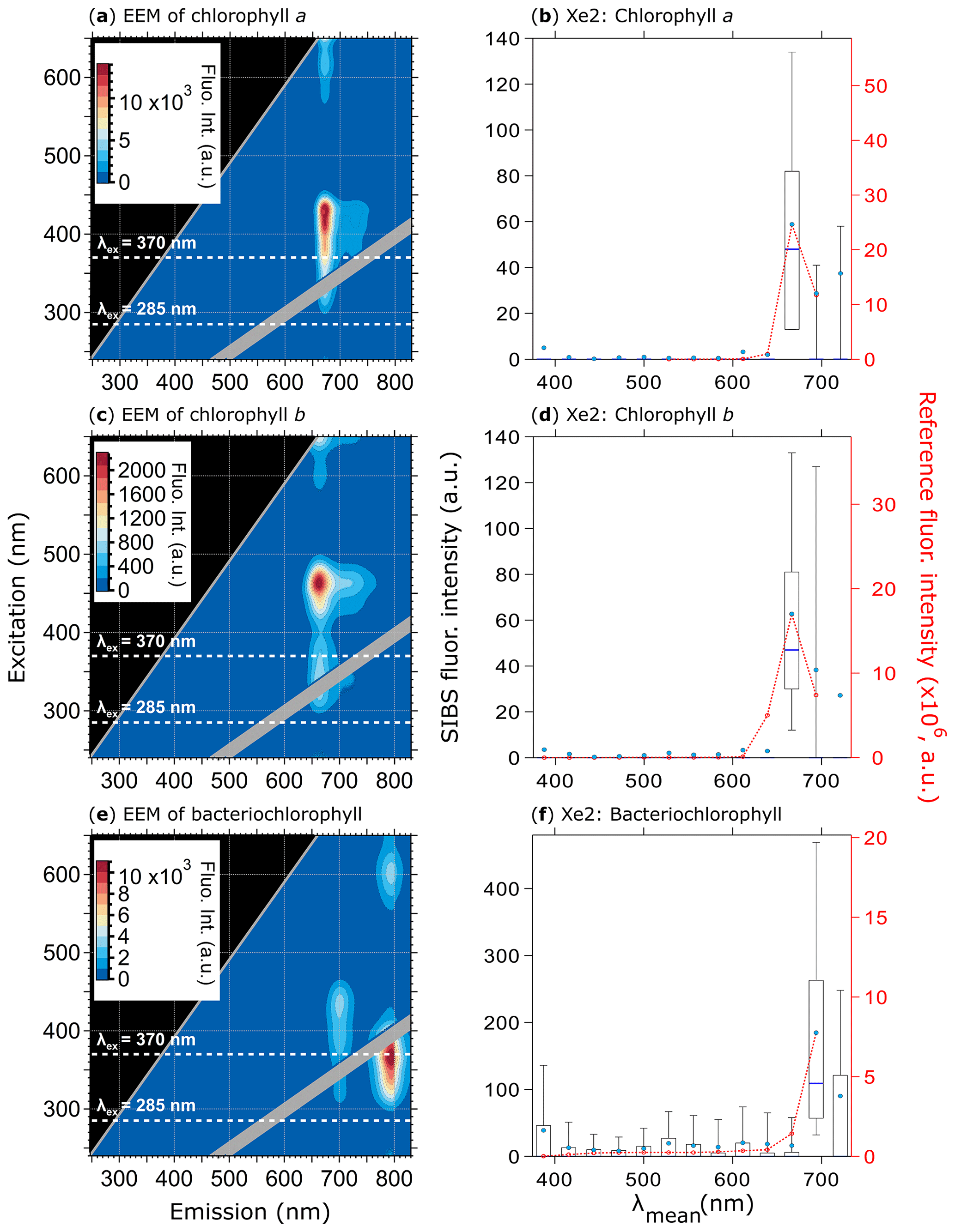
Figure 9Fluorescence emission spectra of three chlorophyll types. Highlighted are EEMs (a, c, e) and spectra at Xe2 (b, d, f) for chlorophyll a (a, b, 370 particles), chlorophyll b (c, d, 585 particles), and bacteriochlorophyll (e and f, 633 particles). Red dashed lines and markers (right axes; right column) are averaged and re-binned reference spectra. Box–whisker plots and EEMs as described in Fig. 7. Size range chlorophyll a and b: 0.5–2 µm, size range bacteriochlorophyll: 0.5–1 µm. Emission spectra at Xe1 are excluded due to a fluorescence artifact caused by solved components from the polymer of the aerosolization bottles (Fig. S11).
The uncorrected spectrum of tryptophan (Fig. S8) highlights the necessity of a spectral correction to compensate for the low detector responsivity within the UV and near-IR bins. If the fluorescence signal of tryptophan remains uncorrected, the spectra are shifted slightly to longer wavelengths (red shifted) due to the low responsivity of channel 2 in comparison to channel 3, resulting in misleading spectral information. For NAD (Fig. 8h, i), the fluorescence intensity values of channel 6 are lowered due the suppressed amplification efficiency in this particular channel as described for blue PSLs (Sect. 4.4.1).
All biofluorophores (except chlorophyll types) were aerosolized as dry powders (see Sect. 2.2) to avoid fluorescence solvatochromism effects (e.g., Johnson et al., 1985). Solvatochromism of fluorophores in aqueous solution – the only atmospherically relevant case – typically shifts fluorescence emissions to longer wavelengths due to the stabilized excited state caused by polar solvents (Lakowicz, 2004). This spectral red shift can be seen in Fig. S9, where the peak maximum for NAD shows a difference of ∼15 nm between a dry and water-solvated state, whereas riboflavin reveals an even higher shift of ∼37 nm. Here, solvatochromism serves as an example for fluorescence spectra that vary substantially as a function of the fluorophore's microenvironments (e.g., solvent polarity, pH, temperature).
Each of the three types of chlorophyll exhibits the weakest emission of all biofluorophores measured within this study; however, the SIBS was able to detect the fluorescence signal at λex=370 nm for all three (Fig. 9). The spectral difference between chlorophyll a and b is only minor at λex=370 nm (Δλ=8.3 nm) for which the spectral resolution of the SIBS is not capable of distinguishing between types (Figs. 9a, b, c, d and S10) (e.g., French et al., 1956; Welschmeyer, 1994). Nevertheless, the SIBS shows the ability to distinguish between chlorophyll a and b and bacteriochlorophyll due to the red shift in the bacteriochlorophyll spectrum (Δλ=28.5 nm at λex=370 nm between chlorophyll a and bacteriochlorophyll). This may provide a further discrimination level regarding algae, plant residue, and cyanobacteria. Bacteriochlorophyll also shows a second and even stronger emission peak at λex=370 nm ( nm) that could help further distinguish it from chlorophyll a and b, but the SIBS spectrometer cannot currently detect this far into the IR (e.g., Rijgersberg et al., 1980; Van Grondelle et al., 1983).
Overall, fluorescence emissions recorded by the SIBS are in good agreement with measured reference spectra. However, care must be taken as to the interpretation of fluorescence emissions covering broad spectral ranges, which span regimes with large differences between individual correction factors (e.g., channel 15, λmean=693.9 nm, Fig. 7l; and channel 2, λmean=330.6 nm, Fig. 8k). For the SIBS, the first two UV detection channels and the last two near-IR channels should be treated with care. Further investigation is required for a careful assessment of how the spectral correction can be applied properly with respect to fluorescent and nonfluorescent atmospheric particles.
4.5 Particle asymmetry measurements
The AF of spherical particles such as PSLs (Fig. 10a, b) and ultrapure water droplets is approximately 10 (Table 3), which is slightly higher than reported values for spherical particles by, e.g., Savage et al. (2017) (AF = ∼5) or Toprak and Schnaiter (2013) (AF = ∼8) using a WIBS. It is noteworthy that the AF of water droplets increases slightly with increasing droplet size and therefore contributes to the mean value (Fig. S12). This effect is most likely based on a decreasing surface tension with increasing droplet size for which the droplet morphology is changed to a more oval shape within the sample flow. A similar effect regarding a potential droplet deformation using an airborne particle classifier (APC) was observed by Kaye et al. (1991). Even if the morphology of ammonium sulfate (crystalline; Fig. 10d) and Fe3O4 (irregular clusters; Fig. 10f) is diverse, the difference in AF is only minor (∼13 and 14; Table 3), indicating that most naturally occurring aerosols (e.g., sea salt, soot, various bacterial, and fungal clusters) will occur in an AF regime between ∼10 and 20. Only rod-shaped carbon nanotubes (110–170 nm diameter, 5–9 µm length) show increased AFs with a mean value of ∼22 (Table 3) at which bacteria would also occur (Fig. 10h). No particles observed exhibited average AF values >25, as would have been expected for, e.g., carbon nanotubes. Because the range of AF values for homogenous particles is relatively broad and the differences between morphologically diverse particle types is only minor (Table 3), a question can be raised regarding to what extent particles could be distinguished based on the AF under ambient conditions. Similar broad AF ranges were found in Healy et al. (2012), measuring sodium chloride, chalk, and several pollen and fungal spores types. As also discussed by Savage et al. (2017), the AF values reported by SIBS and WIBS units should be treated with extreme care.
Table 3Asymmetry factor (AF) values for reference particles. Values are based on the mean of a Gaussian fit applied onto each particle histogram (see also Fig. 10), including 1σ SD.
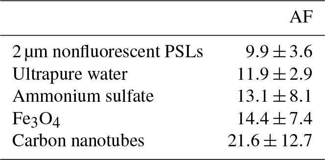

Figure 10Particle asymmetry. Shown are particle density histograms (left column) and microscopy images (right column) for 2 µm nonfluorescent PSLs (a, b, 17 836 particles), ammonium sulfate (c, d, 3496 particles), Fe3O4 (e, f, 65 097 particles), and carbon nanotubes (56 949 particles, g). Scale bar (right column) indicates a length of 10 µm.
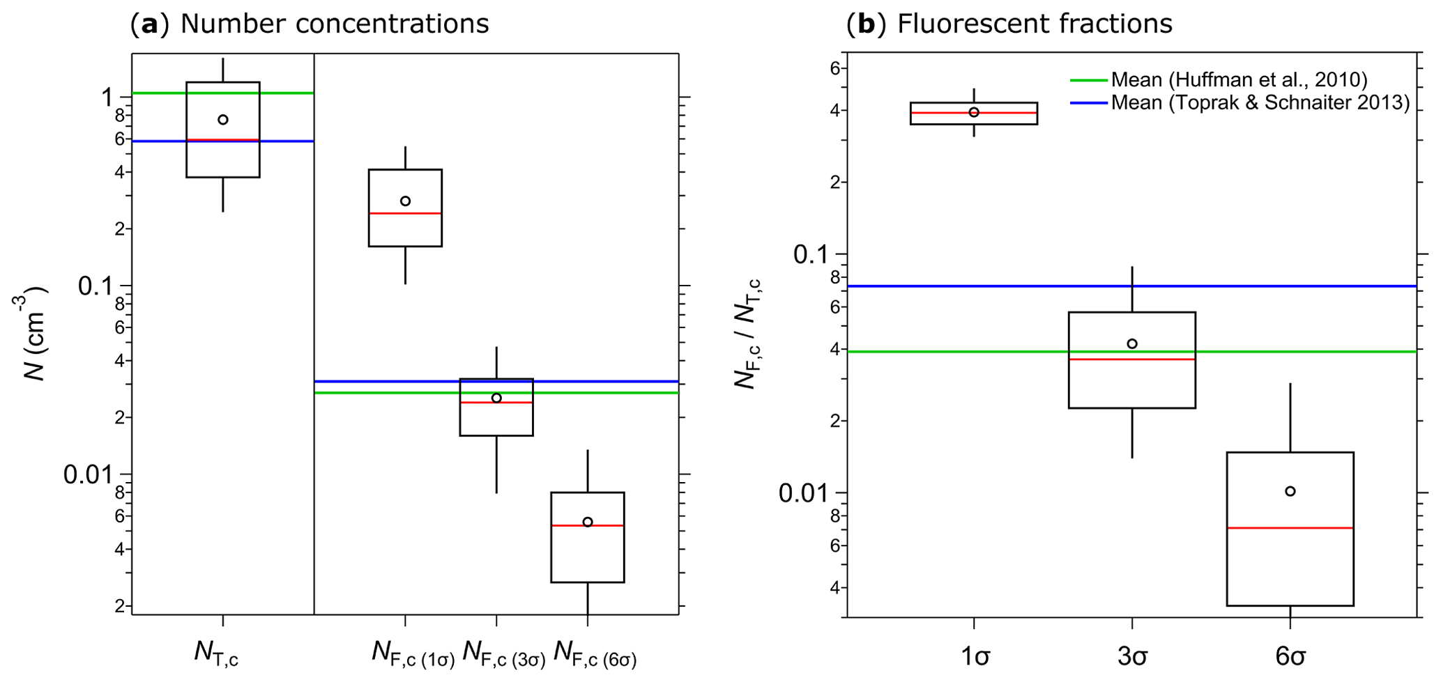
Figure 11Integrated coarse particle (1–20 µm) number concentrations measured between 12 and 18 April 2018 (5 min average) for total particles (NT,c, fluorescent and nonfluorescent) and coarse fluorescent particles (NF,c) after 1, 3, and 6σ SD background signal subtraction (a). The fluorescent fractions of integrated coarse particle number concentrations () at 1, 3, and 6σ SD are shown in (b). Median (red line), mean (black circles); boxes represent the 75th and 25th percentile, and whiskers represent the 95th and 5th percentile (a and b). Data from Huffman et al. (2010) (green lines) and Toprak and Schnaiter (2013) (blue lines) were taken for comparison (a, b).
The validation of asymmetry measurements is challenging due to unavoidable particle and aerosolization effects (e.g., particle agglomeration and spatial orientation within the sample flow) and the lack of standardized procedures for AF calibrations. Measurements performed in this study therefore only serve as a rough AF assignment. Moreover, even if both the SIBS and WIBS use the same technical components for defining AFs, a direct intercomparison cannot be applied due to technical variability (e.g., PMT-related signal-to-noise ratio or the alignment of optical components). Additionally, it is currently unknown how far the 785 nm diode laser of the SIBS affects asymmetry measurements compared to the WIBS using a 635 nm diode laser.
4.6 Initial ambient measurements
Several weeks of initial ambient SIBS measurements were conducted on the roof of the Max Planck Institute for Chemistry in Mainz, Germany. At a nearby building site, Huffman et al. (2010) conducted one of the first ambient UV-APS studies in the year 2006. Moreover, Toprak and Schnaiter (2013) conducted a WIBS-4A study at a comparable site in central Germany from 2010 to 2011. The aim of this brief section is to validate the SIBS-derived key aerosol and fluorescence data as reasonable and relatively consistent with the aforementioned studies. We found a good agreement between the coarse-mode (≥1 µm) number concentrations (NT,c) of the SIBS (NT,c ranging from 0.25 to 1.59 cm−3, with a mean of 0.76 cm−3) and previous data from the UV-APS (mean NT,c: 1.05 cm−3; Huffman et al., 2010) and the WIBS-4A (mean NT,c: 0.58 cm−3; Toprak and Schnaiter, 2013) (Fig. 11a). Furthermore, good agreement was found between coarse-mode fluorescent number concentrations (NF,c) of the SIBS (mean NF,c(3σ): 0.025 cm−3), the UV-APS (mean NF,c: 0.027 cm−3; Huffman et al., 2010), and the WIBS-4A (mean NF,c(3σ): 0.031 cm−3; Toprak and Schnaiter, 2013) (Fig. 11a). Similarly, the fraction of fluorescent particles in the coarse mode () compares well between SIBS (mean : 4.2 %), the UV-APS (mean : 3.9 %; Huffman et al., 2010), and the WIBS-4A (mean : 7.3 %; Toprak and Schnaiter, 2013) (Fig. 11b). Expectedly, a 1σ SD threshold gives much higher SIBS fluorescent fractions of 39.2 %, whereas a 6σ SD threshold corresponds to much lower fluorescent fractions of 1 % (Fig. 11b). Note that no prefect match between our results and the studies by Huffman et al. (2010) and Toprak and Schnaiter (2013) can be expected, since the measurements took place with different sampling setups and during different seasons. Furthermore, the spectrally resolved SIBS data make the definition of fluorescent fraction more complex than for UV-APS and WIBS data (see Sect. 2.6). However, the overall good agreement confirms that the SIBS produces reasonable results in an ambient setting. Further, the single particle fluorescence spectra are reasonable with respect to typical biofluorophore emissions (Pöhlker et al., 2012). Exemplary spectra (λex=285 and 370 nm) of ambient single particles can be found in the Supplement (Fig. S13). An in-depth analysis of extended SIBS ambient datasets is the subject of ongoing work.
Real-time analysis of atmospheric bioaerosols using commercial LIF instruments has largely been restricted to data recorded in only one to three spectrally integrated emission channels, limiting the interpretation of fluorescence information. Instruments that can record resolved fluorescence spectra over a broad range of emission wavelengths may thus be required to further improve the applicability of LIF instrumentation to ambient PBAP detection. Introduced here is the SIBS (DMT, Longmont, CO, USA), which is an instrument that provides resolved fluorescence spectra (λmean=302–721 nm) from each of two excitation wavelengths (λex=285 and 370 nm) for single particles. The current study introduces the SIBS by presenting and experimentally validating its key functionalities. This work critically assesses the strengths and limitations of the SIBS with respect to the growing interest in real-time bioaerosol quantification and classification. It should be noted that the study is an independent evaluation that was not conducted, endorsed, or coauthored by the manufacturer or representatives. Overall, this work confirms a precise particle sizing between 300 nm and 20 µm and particle discrimination ability based on spectrally resolved fluorescence information for several standard compounds.
The SIBS was operated at a low PMT detector amplification setting (610 V) to retain the capacity to detect large or brightly fluorescent particles. It was confirmed, however, that even weak fluorescence signals from 0.53 µm purple PSLs and from small S. cerevisiae fragments (0.5–1 µm) can be clearly distinguished from the background signal. Saturation events were only observed for the polystyrene–detergent signal from relatively large 15 and 20 µm PS-DVB particles. Nevertheless, the fluorescence intensity detection threshold is highly instrument dependent due to the complex interaction of single technical components across individual instruments. For example, xenon 1 exhibited ∼154 % higher irradiance than xenon 2 (both new lamps) due to differences in the properties of xenon emission and the optical filters used. For the xenon lamps used (>4000 h of use), an even higher difference of ∼220 % was observed. Thus, a defined fluorescence detection threshold will most likely change over time due to, e.g., material fatigue. Additionally, variable irradiance properties might significantly contribute to observed differences in performance of similar instrument types (e.g., Hernandez et al., 2016), expressly underlining the need for a fluorescence calibrant applicable across LIF instruments (e.g., Robinson et al., 2017). Nevertheless, to the best of our knowledge, there is currently no standard reference available that fulfills the requirements to serve as a calibrant for multi-channel, multi-excitation LIF instruments. Observations in this study are valid not only for the SIBS, but also for the WIBS-4A and WIBS-NEO, and lead to important implications for the interpretation of particle data. In particular, a particle that exhibits measurable fluorescence in WIBS channel FL1, but only weak fluorescence in channel FL3, could be assigned as an “A-type” particle in one instrument but an “AC-type” particle in an instrument with slightly stronger xenon 2 irradiance. These differences in classification can be extremely important to the interpretation of ambient data (e.g., Perring et al., 2015; Savage et al., 2017).
The PMT used in the SIBS shows a wavelength-dependent sensitivity distribution along all 16 detection channels. To compensate for this characteristic and to be able to use the broadest possible fluorescence emission range, the measured emission spectra were corrected with respect to reference spectra acquired from deuterium and halogen lamps. A spectral correction over a broad emission range also introduces drawbacks, however, that LIF-instrument users should keep in mind while interpreting derived fluorescence information. In particular, the first two (UV) and the last two (near-IR) detection channels should be treated with care because they require larger correction factors compared to adjacent channels. Ultimately, the correction factor and amplification voltages applied to the detector will be experiment specific and will need to be investigated with respect to individual experimental aims. To this extent, possible differences between instruments and important calibrations complicate the concept of the instrument being commercially available. Individual users may desire to purchase the SIBS as a “plug-and-play” detector, but using it without a critical understanding of these complexities would not be appropriate at this time and could lead to inadvertent misinterpretation of the data.
Fluorescence spectra of fluorescent PSLs, amino acids, coenzymes, and flavins measured by the SIBS agree well with corresponding spectra recorded with an off-line reference spectrometer. Thus, the SIBS was shown to be capable of clearly distinguishing between different particle types based on resolved fluorescence information. Furthermore, the extended fluorescence emission range (λem = >700 nm) also enables the SIBS to distinguish chlorophyll a and b from bacteriochlorophyll, potentially opening new possibilities for the detection of, e.g., algae, plant residue, and cyanobacteria.
Particle asymmetry measurements revealed that spherical PSLs have an AF of 9.9(±3.6), whereas other materials (ammonium sulfate, Fe3O4, and carbon nanotubes) show AF values of 13.1(±8.1), 14.4(±7.4), and 21.6(±12.7), respectively. Because differences in measured AF values between morphologically diverse particle types are small and within the ranges of uncertainty for the measurement of a given set of particles, it is questionable how well particles can be distinguished based on the AF as presently measured by the quadrant PMT. Users of SIBS and WIBS instruments should apply extreme care if using AF data. It is also likely that different instrument units may have very different AF responses with respect to this measurement. At a minimum, each individual unit needs to be rigorously calibrated to known particle types to determine if AF values are sufficiently different (e.g., separated by several standard deviations) to justify scientific conclusions based on the metric.
Exemplary ambient data, measured between 12 and 18 April 2018 on the roof of the Max Planck Institute for Chemistry in Mainz (Germany), are consistent with LIF measurement data using a UV-APS (Huffman et al., 2010) and a WIBS-4A in comparable environments (Toprak and Schnaiter, 2013). Total coarse particle number concentrations revealed a mean value of 0.76 cm−3 (1.05 cm−3, Huffman et al., 2010; 0.58 cm−3, Toprak and Schnaiter, 2013) of which ∼4.2 % are considered to be fluorescent using a 3σ SD threshold (3.9 %, Huffman et al., 2010; 7.3 %, Toprak and Schnaiter, 2013), including only particles that show fluorescence emission in at least two adjoining detection channels. Using a 1σ and 6σ SD threshold results in fluorescent fractions of 39.2 % and 1 %, respectively. However, the applicability of different threshold strategies for the SIBS is currently under investigation and needs further verification.
The results suggest that the SIBS has the potential to increase the selectivity of detection of fluorescent biological and nonbiological particles through the use of two excitation wavelengths and 16-channel-resolved fluorescence information in combination with a broad detectable emission range. The applicability of the described methods to ambient datasets is currently under investigation. The data shown here and detailed insights into the technical components used in the SIBS will be broadly beneficial for users of LIF instruments in providing resolved fluorescence information, but also for users of various generations of WIBS and other LIF instruments widely applied within the bioaerosol community.
Mean and median fluorescence spectra for PSLs and biofluorophores (Figs. 7–9, S5, and S6) have been deposited as a Supplement file. For specific data requests, please contact the corresponding authors. High-resolution vector files of figures are presented in the Supplement.
| Acronym or symbol | Description |
| AF | Asymmetry factor |
| APC | Airborne particle classifier |
| CCD | Charge-coupled device |
| DMT | Droplet Measurement Technologies |
| EEM | Excitation–emission matrix |
| λem | Emission wavelength |
| λex | Excitation wavelength |
| IR | Infrared |
| LIF | Light-induced fluorescence |
| N | Particle number concentration (cm−3) |
| NT,c | N of total coarse particles (1–20 µm) |
| NF,c(nσ) | N of fluorescent coarse particles (1–20 µm) at 1, 3, or 6σ |
| NAD | Nicotinamide adenine dinucleotide |
| NAD(P)H | Nicotinamide adenine dinucleotide and nicotinamide adenine dinucleotide phosphate |
| NIST | National institute of standards and technology |
| PBAPs | Primary biological aerosol particles |
| PMT | Photomultiplier tube |
| PAH | Polycyclic aromatic hydrocarbons |
| PSL | Polystyrene latex sphere |
| PS-DVB | Polystyrene divinylbenzene |
| SD | Standard deviation |
| SIBS | Spectral intensity bioaerosol sensor |
| SNR | Signal-to-noise ratio |
| TSPs | Total suspended particles |
| UV | Ultraviolet |
| UV-APS | Ultraviolet aerodynamic particle sizer |
| Vis | Visible light |
| WIBS | Wideband integrated bioaerosol sensor |
The supplement related to this article is available online at: https://doi.org/10.5194/amt-12-1337-2019-supplement.
TKö, JAH, and CP designed the study. TKö performed laboratory and ambient measurements, performed data analyses, and led the writing of the paper. NJS performed laboratory measurements and contributed to data analyses. TKl, DW, JFN, HS, and UP supported the measurements, data analysis, and discussion of the results. JAH and CP supervised the study and paper writing. All authors contributed to data discussion and paper finalization.
The authors declare that they have no conflict of interest.
This work was supported by the Max Planck Society (MPG) and the Max Planck
Graduate Center with the Johannes Gutenberg University
Mainz (MPGC). Financial support for Nicole Savage was provided by the
Phillipson Graduate Fellowship from the University of Denver. We thank
Maria Praß, Mira Pöhlker, Jan-David Förster, Meinrat O. Andreae,
Peter Hoor, Viviane Després, Benjamin Swanson, Jorge Saturno,
Bruna Holanda, Florian Ditas, Daniel Moran-Zuloaga, Björn Nillius,
Jing Ming, Gavin McMeeking, Gary Granger, Alexis Attwood, Greg Kok,
Robert MacAllister, John Walker, Matt Mahin, Matt Freer, Uwe Kuhn,
Minghui Zhang, Petya Yordanova, Naama Lang-Yona, and members of the Mainz
Bioaerosol Laboratory (MBAL) for their support and stimulating
discussions.
The article processing charges for
this open-access
publication were covered by the Max Planck
Society.
Edited by: Charles
Brock
Reviewed by: Ian Crawford and one anonymous referee
Agranovski, V., Ristovski, Z., Hargreaves, M., Blackall, P., and Morawska, L.: Real-time measurement of bacterial aerosols with the UVAPS: performance evaluation, J. Aerosol Sci., 34, 301–317, https://doi.org/10.1016/S0021-8502(02)00181-7, 2003.
Agranovski, V., Ristovski, Z. D., Ayoko, G. A., and Morawska, L.: Performance evaluation of the UVAPS in measuring biological aerosols: Fluorescence spectra from NAD(P)H coenzymes and riboflavin, Aerosol Sci. Tech., 38, 354–364, https://doi.org/10.1080/02786820490437505, 2004.
Baron, P. A. and Willeke, K.: Aerosol fundamentals, Aerosol Meas. Princ. Tech. Appl., 2nd Edn., Wiley, New York, 2001.
Bauer, A. J. R. and Sonnenfroh, D. M.: Spark-induced breakdown spectroscopy-based classification of bioaerosols, in: 2009 IEEE International Workshop on Safety, Security & Rescue Robotics (SSRR), Denver, CO, USA, 1–4, 2009.
Bhangar, S., Huffman, J. A., and Nazaroff, W. W.: Size-resolved fluorescent biological aerosol particle concentrations and occupant emissions in a university classroom, Indoor Air, 24, 604–617, https://doi.org/10.1111/ina.12111, 2014.
Brandrup, J., Immergut, E. H., Grulke, E. A., Abe, A., and Bloch, D. R.: Polymer handbook, Wiley, New York, 1989.
Brosseau, L. M., Vesley, D., Rice, N., Goodell, K., Nellis, M., and Hairston, P.: Differences in detected fluorescence among several bacterial species measured with a direct-reading particle sizer and fluorescence detector, Aerosol Sci. Tech., 32, 545–558, https://doi.org/10.1080/027868200303461, 2000.
Calvo, A. I., Baumgardner, D., Castro, A., Fernández-González, D., Vega-Maray, A. M., Valencia-Barrera, R. M., Oduber, F., Blanco-Alegre, C., and Fraile, R.: Daily behavior of urban fluorescing aerosol particles in northwest Spain, Atmos. Environ., 184, 262–277, https://doi.org/10.1016/j.atmosenv.2018.04.027 2018.
Caruana, D. J.: Detection and analysis of airborne particles of biological origin: present and future, Analyst, 136, 4641–4652, https://doi.org/10.1039/C1AN15506G, 2011.
Chorvat, D. and Chorvatova, A.: Multi-wavelength fluorescence lifetime spectroscopy: a new approach to the study of endogenous fluorescence in living cells and tissues, Laser Phys. Lett., 6, 175–193, https://doi.org/10.1002/lapl.200810132, 2009.
Cooper, W. A.: Effects of coincidence on measurements with a forward scattering spectrometer probe, J. Atmos. Ocean. Tech., 5, 823–832, https://doi.org/10.1175/1520-0426(1988)005<0823:EOCOMW>2.0.CO;2, 1988.
Crawford, I., Ruske, S., Topping, D. O., and Gallagher, M. W.: Evaluation of hierarchical agglomerative cluster analysis methods for discrimination of primary biological aerosol, Atmos. Meas. Tech., 8, 4979–4991, https://doi.org/10.5194/amt-8-4979-2015, 2015.
Crawford, I., Lloyd, G., Herrmann, E., Hoyle, C. R., Bower, K. N., Connolly, P. J., Flynn, M. J., Kaye, P. H., Choularton, T. W., and Gallagher, M. W.: Observations of fluorescent aerosol–cloud interactions in the free troposphere at the High-Altitude Research Station Jungfraujoch, Atmos. Chem. Phys., 16, 2273–2284, https://doi.org/10.5194/acp-16-2273-2016, 2016.
Crouzy, B., Stella, M., Konzelmann, T., Calpini, B., and Clot, B.: All-optical automatic pollen identification: Towards an operational system, Atmos. Environ., 140, 202–212, https://doi.org/10.1016/j.atmosenv.2016.05.062, 2016.
Deepak, A. and Vali, G.: The International Global Aerosol Program (IGAP) plan: Overview (Vol. 1), A. Deepak Pub., Hampton, VA, USA, 1991.
DeRose, P. C.: Standard guide to fluorescence: Instrument calibration and validation, US Department of Commerce, Technology Admininstration, National Institute of Standards and Technology, Gaithersburg, MD, USA, 2007.
DeRose, P. C., Early, E. A., and Kramer, G. W.: Qualification of a fluorescence spectrometer for measuring true fluorescence spectra, Rev. Sci. Instrum., 78, 33107, https://doi.org/10.1063/1.2715952, 2007.
Després, V. R., Huffman, J. A., Burrows, S. M., Hoose, C., Safatov, A. S., Buryak, G., Fröhlich-Nowoisky, J., Elbert, W., Andreae, M. O., Pöschl, U., and Jaenicke, R.: Primary biological aerosol particles in the atmosphere: A review, Tellus B, 64, 15598, https://doi.org/10.3402/tellusb.v64i0.15598, 2012.
Fennelly, M. J., Sewell, G., Prentice, M. B., O'Connor, D. J., and Sodeau, J. R.: The use of real-time fluorescence instrumentation to monitor ambient primary biological aerosol particles (PBAP), Atmosphere, 9, 1, https://doi.org/10.3390/atmos9010001, 2017.
Fernández-Rodríguez, S., Tormo-Molina, R., Lemonis, N., Clot, B., O'Connor, D. J., and Sodeau, J. R.: Comparison of fungal spores concentrations measured with wideband integrated bioaerosol sensor and Hirst methodology, Atmos. Environ., 175, 1–14, https://doi.org/10.1016/j.atmosenv.2017.11.038, 2018.
Foot, V. E., Kaye, P. H., Stanley, W. R., Barrington, S. J., Gallagher, M., and Gabey, A.: Low-cost real-time multiparameter bio-aerosol sensors, Proc. SPIE, 7116, 71160I-12, https://doi.org/10.1117/12.800226, 2008.
French, C. S., Smith, J. H. C., Virgin, H. I., and Airth, R. L.: Fluorescence-spectrum curves of chlorophylls, pheophytins, phycoerythrins, phycocyanins and hypericin, Plant Physiol., 31, 369–374, https://doi.org/10.1104/pp.31.5.369, 1956.
Fröhlich-Nowoisky, J., Kampf, C. J., Weber, B., Huffman, J. A., Pöhlker, C., Andreae, M. O., Lang-Yona, N., Burrows, S. M., Gunthe, S. S., Elbert, W., Su, H., Hoor, P., Thines, E., Hoffmann, T., Després, V. R., and Pöschl, U.: Bioaerosols in the earth system: Climate, health, and ecosystem interactions, Atmos. Res., 182, 346–376, https://doi.org/10.1016/j.atmosres.2016.07.018, 2016.
Fuzzi, S., Andreae, M. O., Huebert, B. J., Kulmala, M., Bond, T. C., Boy, M., Doherty, S. J., Guenther, A., Kanakidou, M., Kawamura, K., Kerminen, V.-M., Lohmann, U., Russell, L. M., and Pöschl, U.: Critical assessment of the current state of scientific knowledge, terminology, and research needs concerning the role of organic aerosols in the atmosphere, climate, and global change, Atmos. Chem. Phys., 6, 2017–2038, https://doi.org/10.5194/acp-6-2017-2006, 2006.
Gabey, A. M., Gallagher, M. W., Whitehead, J., Dorsey, J. R., Kaye, P. H., and Stanley, W. R.: Measurements and comparison of primary biological aerosol above and below a tropical forest canopy using a dual channel fluorescence spectrometer, Atmos. Chem. Phys., 10, 4453–4466, https://doi.org/10.5194/acp-10-4453-2010, 2010.
Gabey, A. M., Vaitilingom, M., Freney, E., Boulon, J., Sellegri, K., Gallagher, M. W., Crawford, I. P., Robinson, N. H., Stanley, W. R., and Kaye, P. H.: Observations of fluorescent and biological aerosol at a high-altitude site in central France, Atmos. Chem. Phys., 13, 7415–7428, https://doi.org/10.5194/acp-13-7415-2013, 2013.
Gosselin, M. I., Rathnayake, C. M., Crawford, I., Pöhlker, C., Fröhlich-Nowoisky, J., Schmer, B., Després, V. R., Engling, G., Gallagher, M., Stone, E., Pöschl, U., and Huffman, J. A.: Fluorescent bioaerosol particle, molecular tracer, and fungal spore concentrations during dry and rainy periods in a semi-arid forest, Atmos. Chem. Phys., 16, 15165–15184, https://doi.org/10.5194/acp-16-15165-2016, 2016.
Guilbault, G. G.: Practical fluorescence, Vol. 3, CRC Press, New York, USA, 1990.
Hairston, P. P., Ho, J., and Quant, F. R.: Design of an instrument for real-time detection of bioaerosols using simultaneous measurement of particle aerodynamic size and intrinsic fluorescence, J. Aerosol Sci., 28, 471–482, https://doi.org/10.1016/S0021-8502(96)00448-X, 1997.
Healy, D. A., O'Connor, D. J., Burke, A. M., and Sodeau, J. R.: A laboratory assessment of the Waveband Integrated Bioaerosol Sensor (WIBS-4) using individual samples of pollen and fungal spore material, Atmos. Environ., 60, 534–543, https://doi.org/10.1016/j.atmosenv.2012.06.052, 2012.
Healy, D. A., Huffman, J. A., O'Connor, D. J., Pöhlker, C., Pöschl, U., and Sodeau, J. R.: Ambient measurements of biological aerosol particles near Killarney, Ireland: a comparison between real-time fluorescence and microscopy techniques, Atmos. Chem. Phys., 14, 8055–8069, https://doi.org/10.5194/acp-14-8055-2014, 2014.
Herbrich, S., Gehder, M., Krull, R., and Gericke, K.-H.: Label-free spatial analysis of free and enzyme-bound NAD (P) H in the presence of high concentrations of melanin, J. Fluoresc., 22, 349–355, https://doi.org/10.1007/s10895-011-0965-5, 2012.
Hernandez, M., Perring, A. E., McCabe, K., Kok, G., Granger, G., and Baumgardner, D.: Chamber catalogues of optical and fluorescent signatures distinguish bioaerosol classes, Atmos. Meas. Tech., 9, 3283–3292, https://doi.org/10.5194/amt-9-3283-2016, 2016.
Hill, S. C., Pinnick, R. G., Niles, S., Pan, Y., Holler, S., Chang, R. K., Bottiger, J., Chen, B. T., Orr, C., and Feather, G.: Real-time measurement of fluorescence spectra from single airborne biological particles, Field Anal. Chem. Tech., 3, 221–239, https://doi.org/10.1002/(SICI)1520-6521(1999)3:4/5<221::AID-FACT2>3.0.CO;2-7, 1999.
Hill, S. C., Mayo, M. W., and Chang, R. K.: Fluorescence of bacteria, pollens, and naturally occurring airborne particles: excitation/emission spectra, ARL-TR-4722, Army Res. Lab. Appl. Phys., Adelphi, MD, USA, 2009.
Hill, S. C., Williamson, C. C., Doughty, D. C., Pan, Y.-L., Santarpia, J. L., and Hill, H. H.: Size-dependent fluorescence of bioaerosols: Mathematical model using fluorescing and absorbing molecules in bacteria, J. Quant. Spectrosc. Ra., 157, 54–70, https://doi.org/10.1016/j.jqsrt.2015.01.011, 2015.
Hinds, W. C.: Aerosol technology: Properties. Behavior, and measurement of Airborne particles, 2nd Edn., Wiley, New York, USA, 1999.
Ho, J.: Future of biological aerosol detection, Anal. Chim. Acta, 457, 125–148, https://doi.org/10.1016/S0003-2670(01)01592-6, 2002.
Holbrook, R. D., DeRose, P. C., Leigh, S. D., Rukhin, A. L., and Heckert, N. A.: Excitation–emission matrix fluorescence spectroscopy for natural organic matter characterization: a quantitative evaluation of calibration and spectral correction procedures, Appl. Spectrosc., 60, 791–799, https://doi.org/10.1366/000370206777886973, 2006.
Huffman, J. A. and Santarpia, J.: Online techniques for quantification and characterization of biological aerosols, Microbiol. Aerosols, 83–114, 2017.
Huffman, J. A., Treutlein, B., and Pöschl, U.: Fluorescent biological aerosol particle concentrations and size distributions measured with an Ultraviolet Aerodynamic Particle Sizer (UV-APS) in Central Europe, Atmos. Chem. Phys., 10, 3215–3233, https://doi.org/10.5194/acp-10-3215-2010, 2010.
Huffman, J. A., Sinha, B., Garland, R. M., Snee-Pollmann, A., Gunthe, S. S., Artaxo, P., Martin, S. T., Andreae, M. O., and Pöschl, U.: Size distributions and temporal variations of biological aerosol particles in the Amazon rainforest characterized by microscopy and real-time UV-APS fluorescence techniques during AMAZE-08, Atmos. Chem. Phys., 12, 11997–12019, https://doi.org/10.5194/acp-12-11997-2012, 2012.
Huffman, J. A., Prenni, A. J., DeMott, P. J., Pöhlker, C., Mason, R. H., Robinson, N. H., Fröhlich-Nowoisky, J., Tobo, Y., Després, V. R., Garcia, E., Gochis, D. J., Harris, E., Müller-Germann, I., Ruzene, C., Schmer, B., Sinha, B., Day, D. A., Andreae, M. O., Jimenez, J. L., Gallagher, M., Kreidenweis, S. M., Bertram, A. K., and Pöschl, U.: High concentrations of biological aerosol particles and ice nuclei during and after rain, Atmos. Chem. Phys., 13, 6151–6164, https://doi.org/10.5194/acp-13-6151-2013, 2013.
Hunter, A. J. R., Morency, J. R., Senior, C. L., Davis, S. J., and Fraser, M. E.: Continuous emissions monitoring using spark-induced breakdown spectroscopy, J. Air Waste Manage., 50, 111–117, https://doi.org/10.1080/10473289.2000.10463982, 2000.
Jaenicke, R.: Abundance of cellular material and proteins in the atmosphere, Science, 308, 73, https://doi.org/10.1126/science.1106335, 2005.
Jeys, T. H., Herzog, W. D., Hybl, J. D., Czerwinski, R. N., and Sanchez, A.: Advanced trigger development, Lincoln Lab. J., 17, 29–62, 2007.
Johnson, I. D., Thomas, E. W., and Cundall, R. B.: Fluorescence solvatochromism of nitrodiphenylhexatrienes, J. Chem. Soc. Farad. T., 81, 1303–1315, https://doi.org/10.1039/F29858101303, 1985.
Jonsson, P. and Tjärnhage, T.: Trends in Biological Detection BT – Bioaerosol detection technologies, edited by: Jonsson, P., Olofsson, G., and Tjärnhage, T., 317–322, Springer New York, New York, NY, 2014.
Kanaani, H., Hargreaves, M., Ristovski, Z., and Morawska, L.: Performance assessment of UVAPS: Influence of fungal spore age and air exposure, J. Aerosol Sci., 38, 83–96, https://doi.org/10.1016/j.jaerosci.2006.10.003, 2007.
Kaye, P. H., Eyles, N. A., Ludlow, I. K., and Clark, J. M.: An instrument for the classification of airborne particles on the basis of size, shape, and count frequency, Atmos. Environ. A-Gen., 25, 645–654, https://doi.org/10.1016/0960-1686(91)90062-C, 1991.
Kaye, P. H., Alexander-Buckley, K., Hirst, E., Saunders, S., and Clark, J. M.: A real-time monitoring system for airborne particle shape and size analysis, J. Geophys. Res.-Atmos., 101, 19215–19221, https://doi.org/10.1029/96JD00228, 1996.
Kaye, P. H., Barton, J. E., Hirst, E., and Clark, J. M.: Simultaneous light scattering and intrinsic fluorescence measurement for the classification of airborne particles, Appl. Optics, 39, 3738–3745, https://doi.org/10.1364/AO.39.003738, 2000.
Kaye, P. H., Stanley, W. R., Hirst, E., Foot, E. V, Baxter, K. L., and Barrington, S. J.: Single particle multichannel bio-aerosol fluorescence sensor, Opt. Express, 13, 3583–3593, https://doi.org/10.1364/OPEX.13.003583, 2005.
Khalaji, M., Roshanzadeh, B., Mansoori, A., Taefi, N., and Tavassoli, S. H.: Continuous dust monitoring and analysis by spark induced breakdown spectroscopy, Opt. Laser. Eng., 50, 110–113, https://doi.org/10.1016/j.optlaseng.2011.10.009, 2012.
Kiselev, D., Bonacina, L., and Wolf, J.-P.: Individual bioaerosol particle discrimination by multi-photon excited fluorescence, Opt. Express, 19, 24516–24521, https://doi.org/10.1364/OE.19.024516, 2011.
Kiselev, D., Bonacina, L., and Wolf, J.-P.: A flash-lamp based device for fluorescence detection and identification of individual pollen grains, Rev. Sci. Instrum., 84, 33302, https://doi.org/10.1063/1.4793792, 2013.
Könemann, T., Savage, N. J., Huffman, J. A., and Pöhlker, C.: Characterization of steady-state fluorescence properties of polystyrene latex spheres using off- and online spectroscopic methods, Atmos. Meas. Tech., 11, 3987–4003, https://doi.org/10.5194/amt-11-3987-2018, 2018.
Lakowicz, J. R.: Principles of fluorescence spectroscopy, Kluwer Academic/Plenum, New York, USA, 2004.
Li, J. K., Asali, E. C., Humphrey, A. E., and Horvath, J. J.: Monitoring cell concentration and activity by multiple excitation fluorometry, Biotechnol. Progr., 7, 21–27, https://doi.org/10.1021/bp00007a004, 1991.
Lorenz, L.: Lysbevægelsen i og uden for en af plane Lysbølger belyst Kugle, Vid. Selsk. Skr., 6, 403–420, 1890.
Ma, Y., Wang, Z., Yang, D., Diao, Y., Wang, W., Zhang, H., Zhu, W., and Zheng, J.: On-line measurement of fluorescent aerosols near an industrial zone in the Yangtze River Delta region using a wideband integrated bioaerosol spectrometer, Sci. Total Environ., 656, 447–457, https://doi.org/10.1016/j.scitotenv.2018.11.370, 2019.
Madelin, T. M.: Fungal aerosols: A review, J. Aerosol Sci., 25, 1405–1412, https://doi.org/10.1016/0021-8502(94)90216-X, 1994.
Mie, G.: Considerations on the optics of turbid media, especially metal sols, Ann. Phys.-Berlin, 25, 377–442, https://doi.org/10.1002/andp.19083300302, 1908.
Moran-Zuloaga, D., Ditas, F., Walter, D., Saturno, J., Brito, J., Carbone, S., Chi, X., Hrabe de Angelis, I., Baars, H., Godoi, R. H. M., Heese, B., Holanda, B. A., Lavric, J. V., Martin, S. T., Ming, J., Pöhlker, M. L., Ruckteschler, N., Su, H., Wang, Y., Wang, Q., Wang, Z., Weber, B., Wolff, S., Artaxo, P., Pöschl, U., Andreae, M. O., and Pöhlker, C.: Long-term study on coarse mode aerosols in the Amazon rain forest with the frequent intrusion of Saharan dust plumes, Atmos. Chem. Phys., 18, 10055–10088, https://doi.org/10.5194/acp-18-10055-2018, 2018.
Nasir, Z., Rolph, C., Collins, S., Stevenson, D., Gladding, T., Hayes, E., Williams, B., Khera, S., Jackson, S., and Bennett, A.: A controlled study on the characterisation of bioaerosols emissions from compost, Atmosphere, 9, 379, https://doi.org/10.3390/atmos9100379, 2018.
O'Connor, D. J., Healy, D. A., and Sodeau, J. R.: The on-line detection of biological particle emissions from selected agricultural materials using the WIBS-4 (Waveband Integrated Bioaerosol Sensor) technique, Atmos. Environ., 80, 415–425, https://doi.org/10.1016/j.atmosenv.2013.07.051, 2013.
O'Connor, D. J., Lovera, P., Iacopino, D., O'Riordan, A., Healy, D. A., and Sodeau, J. R.: Using spectral analysis and fluorescence lifetimes to discriminate between grass and tree pollen for aerobiological applications, Anal. Methods-UK, 6, 1633–1639, https://doi.org/10.1039/C3AY41093E, 2014.
Pan, Y.-L.: Detection and characterization of biological and other organic-carbon aerosol particles in atmosphere using fluorescence, J. Quant. Spectrosc. Ra., 150, 12–35, https://doi.org/10.1016/j.jqsrt.2014.06.007, 2015.
Pan, Y.-L., Hartings, J., Pinnick, R. G., Hill, S. C., Halverson, J., and Chang, R. K.: Single-particle fluorescence spectrometer for ambient aerosols, Aerosol Sci. Tech., 37, 628–639, https://doi.org/10.1080/02786820300904, 2003.
Pan, Y.-L., Hill, S. C., Pinnick, R. G., Huang, H., Bottiger, J. R., and Chang, R. K.: Fluorescence spectra of atmospheric aerosol particles measured using one or two excitation wavelengths: Comparison of classification schemes employing different emission and scattering results, Opt. Express, 18, 12436–12457, https://doi.org/10.1364/OE.18.012436, 2010.
Pelling, A. E., Sehati, S., Gralla, E. B., Valentine, J. S., and Gimzewski, J. K.: Local nanomechanical motion of the cell wall of Saccharomyces cerevisiae, Science, 305, 1147–1150, https://doi.org/10.1126/science.1097640, 2004.
Perring, A. E., Schwarz, J. P., Baumgardner, D., Hernandez, M. T., Spracklen, D. V., Heald, C. L., Gao, R. S., Kok, G., McMeeking, G. R., McQuaid, J. B., and Fahey, D. W.: Airborne observations of regional variation in fluorescent aerosol across the United States, J. Geophys. Res.-Atmos., 120, 1153–1170, https://doi.org/10.1002/2014JD022495, 2015.
Pinnick, R. G., Hill, S. C., Pan, Y.-L., and Chang, R. K.: Fluorescence spectra of atmospheric aerosol at Adelphi, Maryland, USA: Measurement and classification of single particles containing organic carbon, Atmos. Environ., 38, 1657–1672, https://doi.org/10.1016/j.atmosenv.2003.11.017, 2004.
Pöhlker, C., Huffman, J. A., and Pöschl, U.: Autofluorescence of atmospheric bioaerosols – fluorescent biomolecules and potential interferences, Atmos. Meas. Tech., 5, 37–71, https://doi.org/10.5194/amt-5-37-2012, 2012.
Pöhlker, C., Huffman, J. A., Förster, J.-D., and Pöschl, U.: Autofluorescence of atmospheric bioaerosols: spectral fingerprints and taxonomic trends of pollen, Atmos. Meas. Tech., 6, 3369–3392, https://doi.org/10.5194/amt-6-3369-2013, 2013.
Pöschl, U.: Atmospheric aerosols: Composition, transformation, climate and health effects, Angew. Chem. Int. Edit., 44, 7520–7540, https://doi.org/10.1002/anie.200501122, 2005.
Pöschl, U. and Shiraiwa, M.: Multiphase chemistry at the atmosphere–biosphere interface influencing climate and public health in the Anthropocene, Chem. Rev., 115, 4440–4475, https://doi.org/10.1021/cr500487s, 2015.
Reid, J. S., Jonsson, H. H., Maring, H. B., Smirnov, A., Savoie, D. L., Cliff, S. S., Reid, E. A., Livingston, J. M., Meier, M. M., and Dubovik, O.: Comparison of size and morphological measurements of coarse mode dust particles from Africa, J. Geophys. Res.-Atmos., 108, 8593, https://doi.org/10.1029/2002JD002485, 2003.
Reponen, T., Grinshpun, S. A., Conwell, K. L., Wiest, J., and Anderson, M.: Aerodynamic versus physical size of spores: measurement and implication for respiratory deposition, Grana, 40, 119–125, https://doi.org/10.1080/00173130152625851, 2001.
Richards-Kortum, R. and Sevick-Muraca, E.: Quantitative optical spectroscopy for tissue diagnosis, Annu. Rev. Phys. Chem., 47, 555–606, https://doi.org/10.1146/annurev.physchem.47.1.555, 1996.
Rijgersberg, C. P., Van Grondelle, R., and Amesz, J.: Energy transfer and bacteriochlorophyll fluorescence in purple bacteria at low temperature, Biochim. Biophys. Acta, 592, 53–64, https://doi.org/10.1016/0005-2728(80)90113-9, 1980.
Robinson, E. S., Gao, R.-S., Schwarz, J. P., Fahey, D. W., and Perring, A. E.: Fluorescence calibration method for single-particle aerosol fluorescence instruments, Atmos. Meas. Tech., 10, 1755–1768, https://doi.org/10.5194/amt-10-1755-2017, 2017.
Robinson, N. H., Allan, J. D., Huffman, J. A., Kaye, P. H., Foot, V. E., and Gallagher, M.: Cluster analysis of WIBS single-particle bioaerosol data, Atmos. Meas. Tech., 6, 337–347, https://doi.org/10.5194/amt-6-337-2013, 2013.
Ruske, S., Topping, D. O., Foot, V. E., Kaye, P. H., Stanley, W. R., Crawford, I., Morse, A. P., and Gallagher, M. W.: Evaluation of machine learning algorithms for classification of primary biological aerosol using a new UV-LIF spectrometer, Atmos. Meas. Tech., 10, 695–708, https://doi.org/10.5194/amt-10-695-2017, 2017.
Saari, S. E., Putkiranta, M. J., and Keskinen, J.: Fluorescence spectroscopy of atmospherically relevant bacterial and fungal spores and potential interferences, Atmos. Environ., 71, 202–209, https://doi.org/10.1016/j.atmosenv.2013.02.023, 2013.
Saari, S. E., Reponen, T., and Keskinen, J.: Performance of two fluorescence-based real-time bioaerosol detectors: BioScout vs. UVAPS, Aerosol Sci. Tech., 48, 371–378, https://doi.org/10.1080/02786826.2013.877579, 2014.
Savage, N. J. and Huffman, J. A.: Evaluation of a hierarchical agglomerative clustering method applied to WIBS laboratory data for improved discrimination of biological particles by comparing data preparation techniques, Atmos. Meas. Tech., 11, 4929–4942, https://doi.org/10.5194/amt-11-4929-2018, 2018.
Savage, N. J., Krentz, C. E., Könemann, T., Han, T. T., Mainelis, G., Pöhlker, C., and Huffman, J. A.: Systematic characterization and fluorescence threshold strategies for the wideband integrated bioaerosol sensor (WIBS) using size-resolved biological and interfering particles, Atmos. Meas. Tech., 10, 4279–4302, https://doi.org/10.5194/amt-10-4279-2017, 2017.
Schmauss, A. and Wigand, A.: Die Atmosphäre als Kolloid, Vieweg + Teubner Verlag, Wiesbaden, 1929.
Schmidt, M. S. and Bauer, A. J. R.: Preliminary correlations of feature strength in spark-induced breakdown spectroscopy of bioaerosols with concentrations measured in laboratory analyses, Appl. Optics, 49, C101–C109, https://doi.org/10.1364/AO.49.00C101, 2010.
Schumacher, C. J., Pöhlker, C., Aalto, P., Hiltunen, V., Petäjä, T., Kulmala, M., Pöschl, U., and Huffman, J. A.: Seasonal cycles of fluorescent biological aerosol particles in boreal and semi-arid forests of Finland and Colorado, Atmos. Chem. Phys., 13, 11987–12001, https://doi.org/10.5194/acp-13-11987-2013, 2013.
Shaw, S. L., Yeh, E., Bloom, K., and Salmon, E. D.: Imaging green fluorescent protein fusion proteins in Saccharomyces cerevisiae, Curr. Biol., 7, 701–704, https://doi.org/10.1016/S0960-9822(06)00299-5, 1997.
Sinski, J. F. and Exner, J.: Concentration dependence in the spectra of polycyclic aromatic hydrocarbon mixtures by front-surface fluorescence analysis, Appl. Spectrosc., 61, 970–977, https://doi.org/10.1366/000370207781746026, 2007.
Sivaprakasam, V., Lin, H.-B., Huston, A. L., and Eversole, J. D.: Spectral characterization of biological aerosol particles using two-wavelength excited laser-induced fluorescence and elastic scattering measurements, Opt. Express, 19, 6191–6208, https://doi.org/10.1364/OE.19.006191, 2011.
Sodeau, J. R. and O'Connor, D. J.: Chap. 16 – Bioaerosol monitoring of the atmosphere for occupational and environmental purposes, Compr. Anal. Chem., 73, 391–420, https://doi.org/10.1016/bs.coac.2016.02.012, 2016.
Stanley, W. R., Kaye, P. H., Foot, V. E., Barrington, S. J., Gallagher, M., and Gabey, A.: Continuous bioaerosol monitoring in a tropical environment using a UV fluorescence particle spectrometer, Atmos. Sci. Lett., 12, 195–199, https://doi.org/10.1002/asl.310, 2011.
Swanson, B. E. and Huffman, J. A.: Development and characterization of an inexpensive single-particle fluorescence spectrometer for bioaerosol monitoring, Opt. Express, 26, 3646–3660, https://doi.org/10.1364/OE.26.003646, 2018.
Toprak, E. and Schnaiter, M.: Fluorescent biological aerosol particles measured with the Waveband Integrated Bioaerosol Sensor WIBS-4: laboratory tests combined with a one year field study, Atmos. Chem. Phys., 13, 225–243, https://doi.org/10.5194/acp-13-225-2013, 2013.
Twohy, C. H., McMeeking, G. R., DeMott, P. J., McCluskey, C. S., Hill, T. C. J., Burrows, S. M., Kulkarni, G. R., Tanarhte, M., Kafle, D. N., and Toohey, D. W.: Abundance of fluorescent biological aerosol particles at temperatures conducive to the formation of mixed-phase and cirrus clouds, Atmos. Chem. Phys., 16, 8205–8225, https://doi.org/10.5194/acp-16-8205-2016, 2016.
Van Grondelle, R., Hunter, C. N., Bakker, J. G. C., and Kramer, H. J. M.: Size and structure of antenna complexes of photosynthetic bacteria as studied by singlet-singlet quenching of the bacteriochlorophyll fluorescence yield, Biochim. Biophys. Acta, 723, 30–36, https://doi.org/10.1016/0005-2728(83)90005-1, 1983.
von der Weiden, S.-L., Drewnick, F., and Borrmann, S.: Particle Loss Calculator – a new software tool for the assessment of the performance of aerosol inlet systems, Atmos. Meas. Tech., 2, 479–494, https://doi.org/10.5194/amt-2-479-2009, 2009.
Welschmeyer, N. A.: Fluorometric analysis of chlorophyll a in the presence of chlorophyll b and pheopigments, Limnol. Oceanogr., 39, 1985–1992, https://doi.org/10.4319/lo.1994.39.8.1985, 1994.
Yao, M.: Bioaerosol: A bridge and opportunity for many scientific research fields, J. Aerosol Sci., 115, 108–112, https://doi.org/10.1016/j.jaerosci.2017.07.010, 2018.
Ziemba, L. D., Beyersdorf, A. J., Chen, G., Corr, C. A., Crumeyrolle, S. N., Diskin, G., Hudgins, C., Martin, R., Mikoviny, T., and Moore, R.: Airborne observations of bioaerosol over the Southeast United States using a wideband integrated bioaerosol sensor, J. Geophys. Res.-Atmos., 121, 8506–8524, https://doi.org/10.1002/2015JD024669, 2016.
Technical information taken from Dual-FL operation manual, rev. A, 30 NOV 2012; Horiba.
The effective excitation band is defined as a “guaranteed minimum bandwidth” (GMBW), describing the spectral region in which a bandpass filter transmits light relative to the mean wavelength. For example, a GMBW of 14 nm means that light is transmitted in a 7 nm spectral range above and below the mean wavelength.