The Disdrometer Verification Network (DiVeN): a UK network of laser precipitation instruments

Starting in February 2017, a network of 14 Thies laser precipitation monitors (LPMs) were installed at various locations around the United Kingdom to create the Disdrometer Verification Network (DiVeN). The instruments were installed for verification of radar hydrometeor classification algorithms but are valuable for much wider use in the scientific and operational meteorological community. Every Thies LPM is able to designate each observed hydrometeor into one of 20 diameter bins from ≥0.125 to >8 mm and one of 22 speed bins from >0.0 to >20.0 m s⁻¹. Using empirically derived relationships, the instrument classifies precipitation into one of 11 possible hydrometeor classes in the form of a present weather code, with an associated indicator of uncertainty. To provide immediate feedback to data users, the observations are plotted in near-real time (NRT) and made publicly available on a website within 7 min. Here we describe the Disdrometer Verification Network and present specific cases from the first year of observations. Cases shown here suggest that the Thies LPM performs well at identifying transitions between rain and snow, but struggles with detection of graupel and pristine ice crystals (which occur infrequently in the United Kingdom) inherently, due to internal processing. The present weather code quality index is shown to have some skill without the supplementary sensors recommended by the manufacturer. Overall the Thies LPM is a useful tool for detecting hydrometeor type at the surface and DiVeN provides a novel dataset not previously observed for the United Kingdom.

1 Introduction

Precipitation in all its various forms is one of the most important meteorological variables. In the UK, severe precipitation events cause millions of pounds worth of damage every year (Thornes, 1992; Penning-Rowsell and Wilson, 2006; Muchan et al., 2015). The phase of precipitation is also important. In winter, limited resources such as flood defences, ploughs, and grit will be allocated differently based on forecasts of hydrometeor type (Elmore et al., 2015; Gascón et al., 2018, and references therein). Accurate observations and forecasts of precipitation amount and type are therefore essential.

1.1 Motivation for DiVeN

Observations of precipitation are traditionally conducted with networks of tipping-bucket rain gauges (henceforth TBRs) such as the UK Met Office network described in Green (2010). TBR gauges funnel precipitation into a bucket, which tips and empties when a threshold volume is reached. The threshold volume is typically equivalent to 0.2 mm depth of rainfall, which means the TBR has a coarse resolution and struggles to measure low rainfall rates over short intervals. For example, a rain rate of 2.4 mm h⁻¹ would only tip a TBR once every 5 min. Moreover, TBRs cannot detect hydrometeor type, only the liquid equivalent when the solid hydrometeors in the funnel melt naturally or from a heating element. Even liquid precipitation is poorly measured by TBRs. Ciach (2003) analysed 15 collocated TBRs and showed that considerable errors occur between the instruments, inconsistent across time and intensity scales. Finally, TBRs are easily blocked by debris and bird droppings, and the airflow around the instrument has been shown to influence the measurement (Groisman et al., 1994).

Weather radar can observe a large area at high spatial and temporal resolution. Since 1979 the United Kingdom Meteorological Office has operated and maintained a network of weather radars at C-band frequency (5.60–5.65 GHz) which, as of March 2018, consists of 15 radars. The 5 min frequency volume data from each radar are quality controlled and corrected before an estimate of surface precipitation rate is derived. Surface precipitation rate estimates from each radar are then composited into a 1 km resolution product (Harrison et al., 2000).

The first operational weather radars only observed a single polarization (Fabry, 2015). An issue with single-polarization weather radar is that it only provides the radar reflectivity factor for the sample volume. Deriving an accurate quantitative estimate of the equivalent rainfall rate from radar reflectivity factor requires additional knowledge about the size distribution and type of hydrometeors being observed.

Dual-polarimetric weather radars are better able to estimate the type of hydrometeor within a sample volume. Thus, variables derived from the dual-polarimetric returns provide information about the shape, orientation, oscillation, and homogeneity of observed particles (Seliga and Bringi, 1978; Hall et al., 1984; Chandrasekar et al., 1990). This information may be used to infer the hydrometeor type through hydrometeor classification algorithms (HCAs). HCAs combine observed polarimetric variables using prior knowledge of typical values for each hydrometeor type, to identify the most likely hydrometeor species within a sample volume (Liu and Chandrasekar, 2000). Chandrasekar et al. (2013) give an overview of recent work on HCAs.

Starting in mid-2012 and completing early 2018, every radar in the UK Met Office network was upgraded from single to dual-polarization using in-house design and off-the-shelf components, reusing the pedestal and reflector from the original radar systems. To take advantage of the new information and to improve precipitation estimates, an operational HCA was developed within the Met Office, based on work at Météo France (Al-Sakka et al., 2013). While significant amounts of literature have been published on the technical improvement of HCAs (Chandrasekar et al., 2013), the verification of HCA skill has not been discussed as widely. There is a need for more rigorous validation of HCAs and DiVeN was created specifically for the verification of the UK Met Office radar network HCA.

Typically in situ aircraft are used to verify radar HCA (Liu and Chandrasekar, 2000; Lim et al., 2005; Ribaud et al., 2016). Instrumented aircraft flights such as the Facility for Airborne Atmospheric Measurements (FAAM) take a swath volume using 20 Hz photographic disdrometer instruments (Abel et al., 2014). However there is no fall speed information, which distinguishes hydrometeor type with high skill due to distinct particle density differences (Locatelli and Hobbs, 1974). The lack of fall speed information on FAAM instruments means that the 1200 images collected in every minute of flight must be visually analysed manually or with complex image recognition algorithms. The major disadvantage with FAAM data is the sparsity of cases due to the expense of operating the aircraft.

Therefore, in situ surface observations must be utilized to expand the quantity of comparison data. A larger dataset allows bulk verification statistics to be performed on radar HCAs. Here we introduce a new surface hydrometeor type dataset and examine the skill of the dataset, independently of any radar instruments.

1.2 Precipitation measurement with disdrometers

A disdrometer is an instrument which measures the drop size distribution of precipitation over time. The drop size distribution (henceforth DSD) of precipitation is the function of drop size and drop frequency. Jameson and Kostinski (2001) provide an in-depth discussion on the definition of a DSD. Disdrometers typically record drop sizes into bins of nonlinearly increasing widths due to the accuracy reducing with increasing values.

The disdrometer is also a useful tool for verifying radar hydrometeor classification algorithms. Hydrometeor type can be empirically derived using information about the diameter and fall speed of the particle, which the Thies laser precipitation monitor (LPM) instrument used in DiVeN is able to measure. The Gunn–Kinzer curve (Gunn and Kinzer, 1949) describes the relationship between raindrop diameter and fall speed. As diameter increases, the velocity of a raindrop increases asymptotically. Other velocity–diameter relations have been shown in the literature for snow, hail, and graupel, which are well described in Locatelli and Hobbs (1974).

At of the time of writing this publication, operational networks of disdrometers are uncommon, with the notable exceptions of Canada (Sheppard, 1990) and Germany. Networks of disdrometers solely for research purposes have been frequently deployed for short periods of time. From March 2009 to July 2010 (16 months), 16 disdrometers were placed on rooftops within 1 km by 1 km on the campus of the Swiss Federal Institute of Technology in Lausanne to study the inter-radar pixel variability in rainfall (Jaffrain et al., 2011). Another example of research using networked disdrometers is the Midlatitude Continental Convective Clouds Experiment (MC3E) (Jensen et al., 2016), which utilized 18 Parsivel-1 disdrometers and seven 2DVDs (two-dimensional video disdrometers) within a 6 km radius of a central facility near Ponca City, Oklahoma. The project lasted for 6 weeks (22 April through 6 June 2011). DiVeN has an initial deployment phase of 3 years with a high expectation of renewal, which enables unique long-term research to be conducted with the data.

1.3 Paper structure

This paper describes DiVeN and demonstrates the data products of the Thies LPM instruments being used. The first part of the paper provides a technical description of the disdrometer instruments used in the network, the locations chosen to host the instruments, and data management in the network. Case studies from the first 12 months of DiVeN observations are then discussed. The case studies include rain–snow transitions in the 2017 winter storm named Doris, a convective rainfall event, and graupel observations. These events will provide an illustrative analysis of the observations being produced by all the individual disdrometer instruments within DiVeN. Enhanced scrutiny will be placed on the performance of the present weather code because this variable will be used to verify the Met Office radar HCAs.

2 Thies Clima laser precipitation monitor

2.1 Specification

The instruments used in DiVeN (see Fig. 1) are the Thies^™ laser precipitation monitor (LPM), model number 5.4110.00.200, which is described in detail in Adolf Thies GmbH & Co. KG (2011). To make observations the instrument utilizes an infrared (785 nm) beam with dimensions of 228 mm × 20 mm × 0.75 mm, a total horizontal area of 45.6 cm². The infrared beam is emitted from one end of the instrument and is directed to the other. A photodiode and signal processor determine the optical characteristics including optical intensity, which is reduced as a particle falls through the beam. The diameter of the hydrometeor is inferred by the maximum amplitude of the signal reduction and the speed of the hydrometeor is estimated by the duration of the signal reduction. Figure 1 in Löffler-Mang and Joss (2000) describes a similar instrument (Parsivel-1) with the same observing principle and is an excellent visualization of the technique which is employed by the Thies LPM. The signal processing claims to detect and remove particles that fall on the edge of the beam: “the measured values are processed by a signal processor (DSP), and checked for plausibility (e.g. edge hits).” No further details are given by the manufacturer. The instrument is able to allocate individual hydrometeors into 20 diameter bins from 0.125 to >8 mm and 22 speed bins from >0.0 to >20 m s⁻¹.

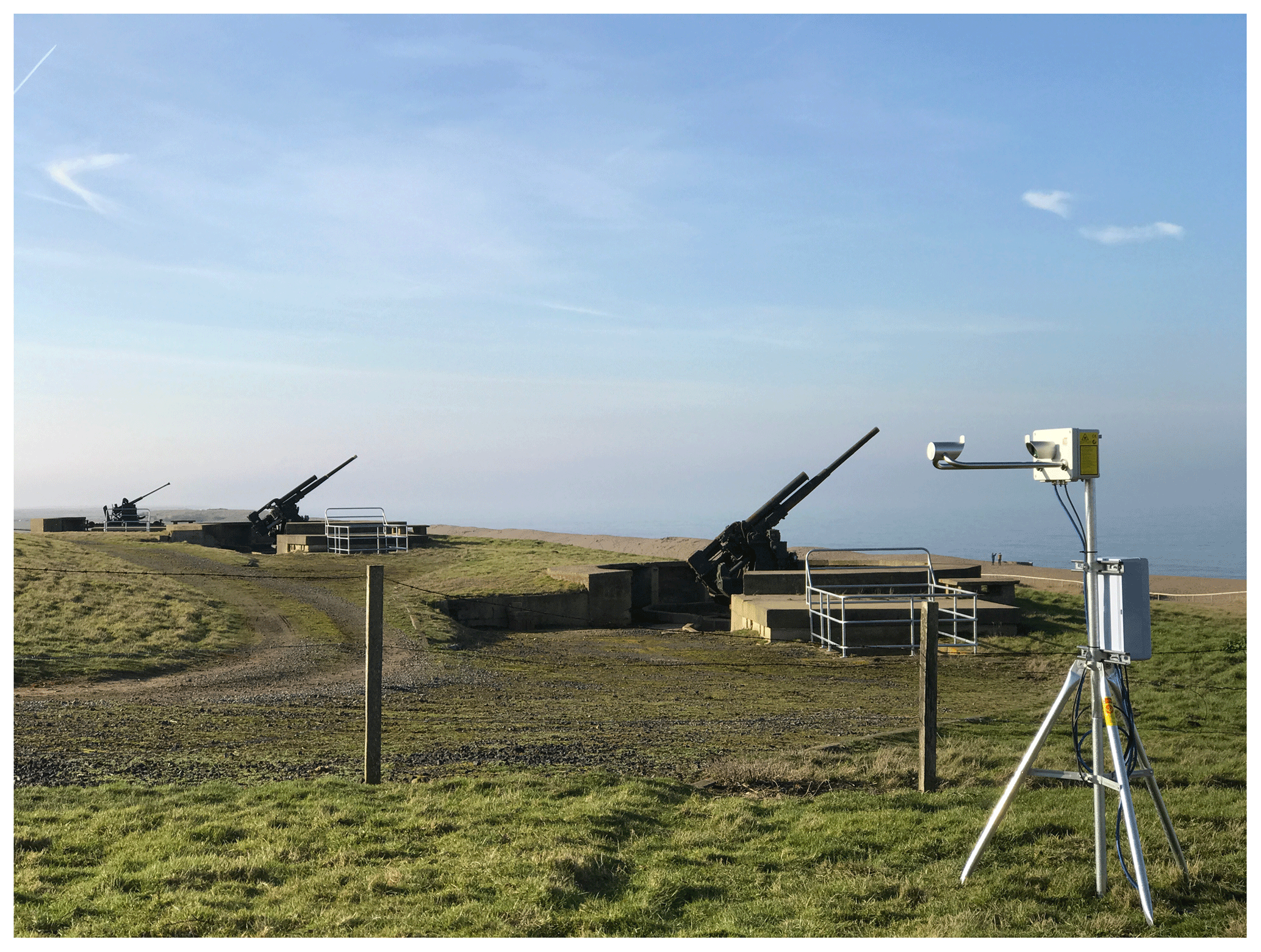
Figure 1 A DiVeN Thies LPM located at Weybourne Observatory in Weybourne, East Anglia, UK, which is an Atmospheric Measurement Facility (AMF) site, part of the National Centre for Atmospheric Science (NCAS).

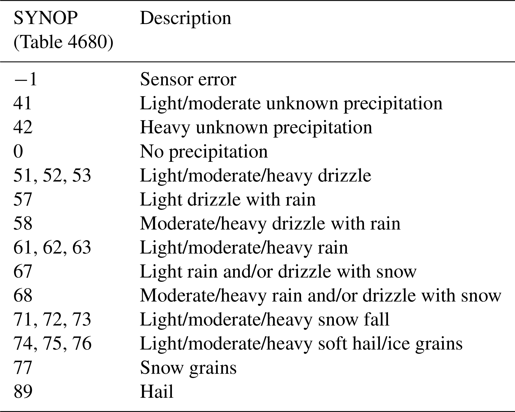
The Thies disdrometer performs additional calculations on the incoming data which it attaches to the Telegram 4 serial output. Table 1 provides details of the variables and the range of possible values that the instrument is capable of recording. The quantity, intensity, and type of precipitation (drizzle, rain, snow, ice, grains, soft hail, and hail as well as combinations of multiple types) are calculated. Hydrometeor type is recorded as a present weather code. Table 2 lists all of the WMO Table 4680 present weather codes that the Thies laser precipitation monitor is capable of recording. The present weather code is encoded as a number between 1 and 99, which has a corresponding description of the weather using the standardized codes from the World Meteorological Organization Table 4860 (WMO, 1988). The present weather descriptors cover most hydrometeor types but not all; graupel is not explicitly mentioned, for example.

Table 1 Variable output from the Thies laser precipitation monitor (LPM).

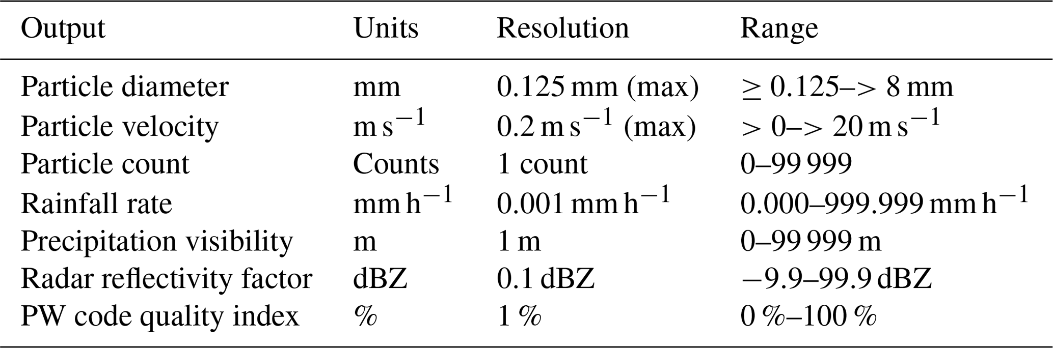
Table 2 World Meteorological Organization (WMO) synoptic present weather codes (Table 4680) output by the Thies laser precipitation monitor (LPM).

Hydrometeor type is inferred by the instrument, using empirical relationships between hydrometeor size and fall speed. The diameter–fall speed relation described in Gunn and Kinzer (1949) is the only relationship cited in the instrument manual but it is expected that further relationships are used for solid precipitation, undisclosed by the manufacturer. Section 4 of this paper will qualitatively test the skill of the present weather code regardless of the algorithm it uses, since the exact method of derivation is not known.

Lastly, the present weather code quality index (Table 1) is calculated based on the number of particles within each hydrometeor class. Thies do not recommended using the quality index without additional temperature and wind sensors which can be added to the disdrometer (Marc Hillebrecht, Adolf Thies GmbH & Co. KG, personal communication, 2017). Although DiVeN does not employ the additional sensors, the quality index is still published and can be a useful indicator as shown in Sect. 4.1.

2.2 Limitations

Tapiador et al. (2016) performed a physical experiment with 14 laser disdrometers (Parsivel-1) placed in close proximity (within 6 m²) on the roof of a building in Toledo, Spain. Precipitation characteristics were calculated for one disdrometer's data, then for two instruments' combined data, and so on until all 14 disdrometers' data were used. The aim was to test how many disdrometers' data were needed for the precipitation parameters to asymptote towards a stable value. It was found that a single disdrometer could underestimate instantaneous rain rate by 70 %. Tapiador et al. (2016) proposed that large drops contribute disproportionately to the rain rate and that instantaneous measurements have a lower chance of measuring large drops because they are sparsely populated. The DiVeN disdrometers have a shortest temporal resolution of 1 min, which alleviates some of the sampling issues by allowing time for larger droplets to be observed.

Hydrometeor type observations are less affected by the aforementioned sample size limitations as the dominant type can be estimated from a relatively small sample of the total precipitation. Theoretically only one hydrometeor needs to be sampled by the disdrometer to determine hydrometeor type. The hydrometeor type accuracy is only as good as the diameter and fall speed measurements. In reality, the accuracy of the diameter and fall velocity measurements for a single particle are not accurate enough to determine the dominant hydrometeor phase from an instantaneous measurement. Furthermore, the fall velocity and diameter of small hydrometeors may be indistinguishably similar for several hydrometeor types when observed by the disdrometer. Similar to the results of Smith (2016) for rainfall rate, the largest particles also give the strongest indication of hydrometeor type. This is because fall velocity is related to the density of the particle multiplicatively (Gunn and Kinzer, 1949); i.e. the difference in fall speed for a 5 mm raindrop and a 5 mm snow aggregate is large compared with the difference between a 0.5 mm raindrop and 0.5 mm ice crystal. Therefore the disdrometer can determine with greater confidence the type of hydrometeor when the hydrometeors are larger.

If the sample size of the instrument were larger and thus could count more particles at a faster rate, other limitations would occur. The instrument relies on observing one particle in the beam at any given time; the optical intensity of the beam must return to normal (no obstruction) for maximum confidence of speed observations. If two hydrometeors partially overlap vertically as they fall through the beam, the disdrometer will observe a double dipped reduction in optical intensity which the signal processor must account for. Similarly for diameter, if two hydrometeors fall through the beam simultaneously, the disdrometer will observe a hydrometeor twice as large at the same speed. The sample area is thus limited to reduce the possibility of overlapping particles. Again, Fig. 1 in Löffler-Mang and Joss (2000) is an excellent diagram to aid the understanding of this limitation.

The chance of two drops being in the disdrometer at the same time is unlikely except at extremely high precipitation rates. To examine this, a Poisson distribution test is applied using the sampling volume of the disdrometer with increasing drop concentrations. Figure 2 shows that precipitation rates of greater than 10 000 drops min⁻¹ are required before the probability of simultaneous drops in the beam occurring becomes non-negligible. There is a 0.09 % chance of two or more drops in the beam simultaneously for 10⁴ drops min⁻¹ observed by the disdrometer; one in every 1075 drops. For 10⁵ drops min⁻¹ observed by the disdrometer there is a 7 % chance of two or more drops in the beam simultaneously; one in every 14 drops. For context, a drop count of 12 000 observed by a disdrometer located at NFARR Atmospheric Observatory, Chilbolton, England, in March 2017 (see Sect. 4.2) was equivalent to 22 mm h⁻¹. Rain rates approaching 100 mm h⁻¹ would be necessary for the chance of two drops existing in the beam simultaneously to be non-negligible. Such rainfall rates are extremely rare in the UK.

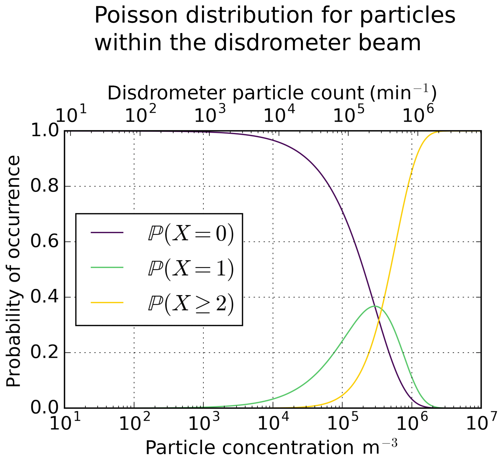
Figure 2 Probability of X number of drops residing within the disdrometer beam for a given drop concentration. If two or more drops are within the beam simultaneously, data quality can be reduced. More than 12 000 drops m⁻³ (equivalent to 10 000 drops min⁻¹ recorded by the disdrometer^*) are required before the probability of two or more drops occurring in the beam simultaneously becomes non-negligible. As such, any events with more than 10 000 drops observed per minute should be treated as less reliable. ^* Drops falling through the disdrometer beam assume a 3 m s⁻¹ fall velocity, which from Gunn and Kinzer (1949) is a particle of approximately 0.8 mm diameter, typically the average size observed for a moderate rainfall event. Droplet breakup on the housing of the Thies LPM is not factored into this test.

3 Description of the network

3.1 DiVeN locations

Disdrometers have similar site specification requirements as other precipitation instruments. Ideally a flat site with no tall objects or buildings nearby that can cause shadowing, and steps taken to minimize the splash of liquid droplets from the surrounding ground into the instrument. To this end, Thies recommends that the instrument be mounted on a 1.5 m pole above a grassy surface. A grassy surface also minimizes convective upwelling from solar heating of the ground – a particular problem for concrete surfaces – which can slow hydrometeor fall speeds and create turbulence. Turbulence from buildings should also be avoided if possible since it acts to break larger particles into smaller particles, resulting in skewed drop size distributions.

The locations chosen for DiVeN cover a variety of geophysical conditions such as mountain peaks, valleys, and flat regions, as well as inland and coastal sites. The locations also cover the full breadth of the climatology of precipitation totals and hydrometeor types in the UK (Fairman et al., 2015) with sites in wetter (Wales) and drier (East Anglia) regions as well as sites in warmer (southern England) and colder (northern Scotland) climates.

Table 3 Site location descriptions of disdrometers in the Disdrometer Verification Network.

The typical range at which the Met Office radar HCA product will need to perform is <120 km (maximum range used to produce surface rainfall rate composite). For the disdrometers to be representative when verification work is performed, the instruments in DiVeN are located at varying ranges from Met Office radars. Figure 3 shows the DiVeN site locations and the Met Office radar locations for comparison. Table 3 gives an overview of each site in DiVeN, including the coordinates, height above mean sea level, and terrain characteristics.

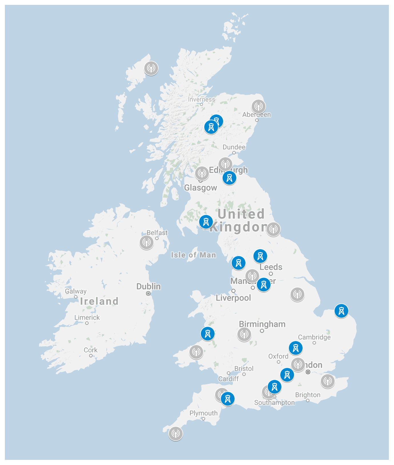
Figure 3 Instrument locations that make up the Disdrometer Verification Network (DiVeN) as of September 2018. Grey icons are the operational Met Office radars as well as the Met Office research radar at Wardon Hill. Map data © 2018 GeoBasis-DE/BKG (© 2009), Google, Inst. Geogr. Nacional.

Two instruments are located 10 m apart at NFARR Atmospheric Observatory in Chilbolton. These two instruments form part of an extended observational period of 12 months where their performance will be assessed against several other precipitation sensors located at the same site. A separate paper will be produced to address the results of this dual-instrument study.

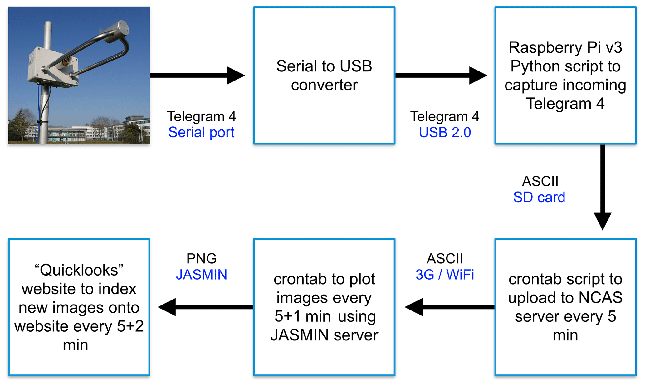
Figure 4 Flow chart of the sequence of data in the Disdrometer Verification Network. The instrument outputs a Telegram 4 format serial ping every minute, which is then captured by a Raspberry Pi (v3) running a Python script. The Python script then saves the file to the built-in SD card as an ASCII.txt. Separate BASH scripts upload the new files every 5 min (xx:05, xx:10, xx:15) to an NCAS server, which JASMIN then reads to plot the data (xx:06, xx:11, xx:16). The website indexes for new images at xx:07, xx:12, xx:17, and so on. Thus the time taken for the xx:00 to xx:05 data to reach the website is 2 min.

3.2 Installation

The main installation campaign occurred in February 2017 for nine instruments. The Holme Moss site was installed shortly after in March, followed by Cairngorm and Feshie in June 2017. Dunkeswell is a Met Office site which was added to the network via a Raspberry Pi with 3G dongle being appended in July 2017. The last instrument to be installed was at Coverhead Estate in the Yorkshire Dales in December 2017, as a collaboration with Water@Leeds https://water.leeds.ac.uk/ (last access: 7 August 2019).

Installation took around 2 h at each site and consisted of anchoring the tripod to the ground, attaching the disdrometer and data logging box, plugging the disdrometer cables into the power strip and the Raspberry Pi, and cutting the power strip cable to length for the site. The installation was designed to be “as plug and play as possible”. Wiring of plugs, data, and power cables onto the disdrometer and coding of the Raspberry Pi were all completed in a lab before arriving at the site.

3.3 DiVeN costs and environmental impact

Each site required the following components to support the disdrometer: Davis Instruments^® tripod (GBP 100, http://www.davisnet.com/product_documents/weather/manuals/07395-299_IM_07716.pdf, last access: 7 August 2019), IP67-rated box (GBP 25, https://www.timeguard.com/products/safety/weathersafe-outdoor-power/outdoor-multi-connector-box, last access: 7 August 2019), Raspberry Pi 3 Model B (GBP 30, https://www.raspberrypi.org/products/raspberry-pi-3-model-b/, last access: 7 August 2019), and a generic RS-485 to USB converter (GBP 12). Therefore the total cost per site for hardware was GBP 167. A total of 200 m of power/data cable and tools required for the installation cost an additional GBP 270 and GBP 60 respectively. Some sites rely on a 3G dongle to upload data. The dongles themselves were free when purchased with a single-use data allotment. The total cost of hardware and equipment to build DiVeN amounted to GBP 2500.

The Thies Clima instrument is power rated at a maximum of 750 mA at 230 v. No typical usage has been measured but should the maximum be continuous, then the annual consumption would be 1500 kWh per year, or GBP 190 per year at average UK electricity costs (valid March 2018). In reality the power consumed is subjectively known to be much less than the maximum rating.

Most sites use existing networks at their sites for uploading data to the NCAS server, but those with 3G dongles have an ongoing cost of GBP 75 per year for a yearly data plan. There are eight sites using 3G dongles; hence the ongoing annual cost is GBP 600.

The emissions from the first 3700 km journey in a diesel van were approximately 966 kg of CO₂ and 1.74 kg of NO_x + PMs (nitrogen oxides + particulate matters). Ongoing power consumption for 13 sites (the Druim nam Bo (Feshie) site is powered off-grid by solar and wind) at the aforementioned maximum rating would be 7150 kg of CO₂ annually (using the UK average of 0.367 kg kWh⁻¹, valid October 2017). In reality the power consumption is less and the UK average kg kWh⁻¹ is gradually decreasing over time. Computational energy consumed by DiVeN is nearly unquantifiable; the data hosting, processing, and analysis were carried out on shared systems (National Centre for Atmospheric Science server, JASMIN server), so the fractional consumption is difficult to estimate.

3.4 Data acquisition and management

The disdrometer data are read through a serial port by a Raspberry Pi, which executes a Python script to receive and digest the Telegram 4 format data. The Python code performs file management with timestamps taken from the Raspberry Pi internal clock (set over IP) and backs up files to a memory card into a directory specific to the date. Separate programming triggers the uploading of new files in the “today” directory to an NCAS server every 5 min over Secure File Transfer Protocol (SFTP). At 01:00 UTC each day, the Raspberry Pi attempts to upload any remaining files in the directory of the previous day. At 02:00 UTC each day, the Raspberry Pi attempts to upload files from the directory for 7 d ago as a backup command in the event that no connection could be made at the time. Only new files that do not already exist on the NCAS server are uploaded to avoid duplication. The entire directory of data for a single day is compressed using tar gunzip, 8 d after it is recorded. A support script exists to keep the processing and uploading scripts running and self-regulating. The support script checks that the processing script is running; if not, it will issue a command to start the processing script again. This means that the data acquisition script will be reattempted if an exit error occurs. In the event of a power loss the Raspberry Pi will start up and initiate all of the required scripts itself when power is restored, without user intervention.

Each disdrometer produces 3.2 MB of ASCII .txt files per day but this can be compressed significantly. A total of 10 years of continuous minute-frequency disdrometer data (5.3 million minutes) can be compressed to as small as 400 MB.

3.5 Open-access website

Data are uploaded to an NCAS server every 5 min. Plotting scripts are initiated 1 min after the upload. An additional minute later, a QuickLook system indexes the target directories for new images and displays them on the public website. The public website can be accessed here: https://sci.ncas.ac.uk/diven/ (last access: 7 August 2019). Data can currently be downloaded from NCAS upon request to the lead author. At the end of the first DiVeN deployment phase (early 2020) all data collected by DiVeN will be archived into netCDF at the Centre for Environmental Data Analysis (CEDA).

3.6 DiVeN users

Although the data from DiVeN will be used for radar verification, there are many other uses for the data. Several stakeholders have used DiVeN data. Met Office operational forecasters are able to see live hydrometeor type data and compare with numerical weather prediction forecasts to adjust their guidance. Second, there are some research projects at the University of Leeds being carried out. This includes research on DSD characteristics in bright band and non-bright band precipitation, calibration work with the NCAS X-band polarimetric (NXPol) radar in Cumbria, England, for the Environment Agency (EA), and flood forecasting research with the Water@Leeds project. Other institutions have also used DiVeN data; The University of Dundee and the Scottish Environment Protection Agency (SEPA) are conducting work on snowmelt and the University of Reading may use DSD information from the Reading University Atmospheric Observatory (RUAO) disdrometer to study aerosol sedimentation rates. Finally, the wind turbine manufacturer Vestas has used annual DSD data to evaluate models of blade-tip drag to improve turbine efficiency. The applications of disdrometer data are broad and cover many fields. The authors intend that this publication combined with the open accessibility of data will inspire new uses of DiVeN observations.

3.7 Performance of DiVeN in the first year

Figure 5 shows the uptime of each site in DiVeN in the order that they were installed. Generally the uptime of the network has been good for the period shown, with most sites uploading more than 95 % each day. A few sites have not been as good but this was mostly anticipated. In particular the Druim nam Bo site at 900 m a.m.s.l. in the Scottish Highlands has poor upload percentages. The 3G signal is weak at the site and a signal booster was added in January 2018. Furthermore the site is powered by a small wind turbine and solar panel, which became rimed in ice during the winter (Fig. 6). Although these issues were anticipated, the site was still chosen because it can provide cases of solid hydrometeors nearly all year round, in a terrain which is notoriously difficult for radar performance. Radar hydrometeor classification will be particularly difficult at this location and thus the site will provide a “worst-case scenario” for radar HCA verification work.

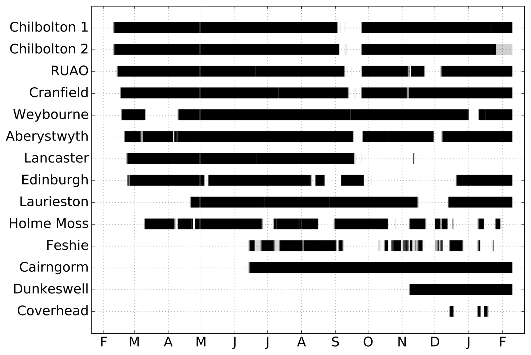
Figure 5 Daily upload performance of DiVeN in the first 365 d of operation. Black indicates 100 % upload (1440 files in a day), and white indicates 0 % upload.

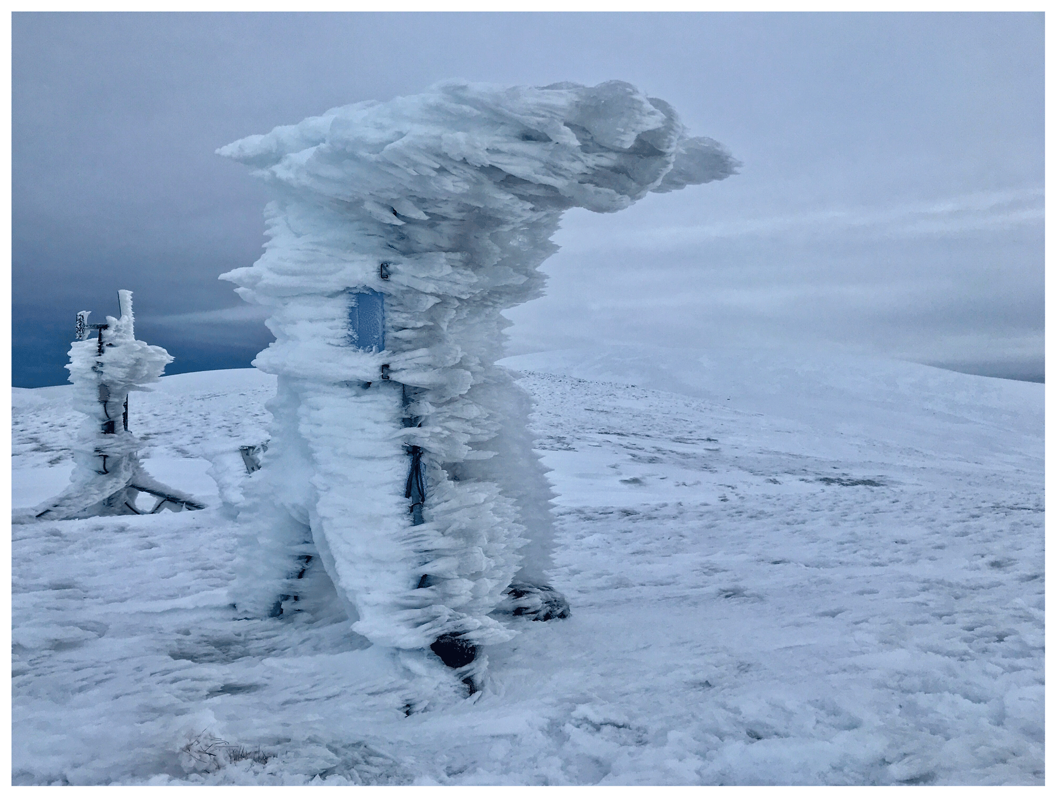
Figure 6 Disdrometer at Druim nam Bo, Scotland, covered in rime in January 2018. The instrument was still receiving power and recording nullified (no beam received by optical diode) data, which it interpreted as a “sensor error” (−1) present weather code.

Holme Moss is a remote site at relatively high altitude and uses satellite broadband, which has been somewhat unreliable; however the amount of data stored on the Raspberry Pi may be higher than depicted in Fig. 5, which was created based from data successfully uploaded to the NCAS server. Furthermore, the data are being archived on the University of Manchester's system at Holme Moss and this is known to be a much more complete dataset, which will be transferred to the NCAS servers in the future.

There were several unanticipated downtime periods. Weybourne had to be moved for construction work at the field site and was without power for approximately 1 month in March 2017. In late April 2017, the NCAS server blacklisted all disdrometer IP addresses and these had to be manually whitelisted. This was detected and resolved within 8 d. The 7 d backup upload filled in the majority of the missing data but the eighth day prior to the issue being fixed was never reattempted because of the design of the code discussed in Sect. 3.4.

The largest unanticipated downtime occurred in September 2017. An issue arose with the disdrometers being unable to record any new data, in the order that they were installed. A total of 2 GB of free space remained on the SD cards; however there was a (previously unknown) limit to the number of files that can be saved to certain card formats regardless of the space remaining. The issue was fixed by the creation of a new script which merged old files together. The script had to be added to all of the Raspberry Pi's in the network. The issue was detected after the first four DiVeN disdrometer installations failed sequentially, so the failure of other sites in the network was anticipated and mitigated. This can be seen in Fig. 5 as a stepped-failure starting with the Chilbolton 1 instrument in September 2017.

Some further issues occurred which were avoidable. Laurieston was disconnected from power whilst closing the data logger box after the installation, which meant it was offline for the first 2 months until the site could be visited again. Similarly during the Dunkeswell installation in July 2017 the serial data cable was damaged, which could not be fixed until November 2017. The Raspberry Pi at Lancaster was not reconnected after the aforementioned file number problem in September 2017.

Although several problems have arisen with the Disdrometer Verification Network in the first 12 months, the network manager and site owners have been, on the whole, quick to respond to these issues, which has minimized downtime. DiVeN is in an ideal state for long-term data collection as it has been designed with few potential failure points and with several backup methods in place in the event of a failure.

4 Case studies

The following sections subjectively analyse the skill of the disdrometer instrument for classifying hydrometeor type. Three types are discussed here: snow from winter storm Doris, an intense rainfall event at NFARR Atmospheric Observatory, and a graupel shower at the Reading University Atmospheric Observatory. NFARR Atmospheric Observatory instrument data were sourced from Science and Technology Facilities Council et al. (2003) and Agnew (2013).

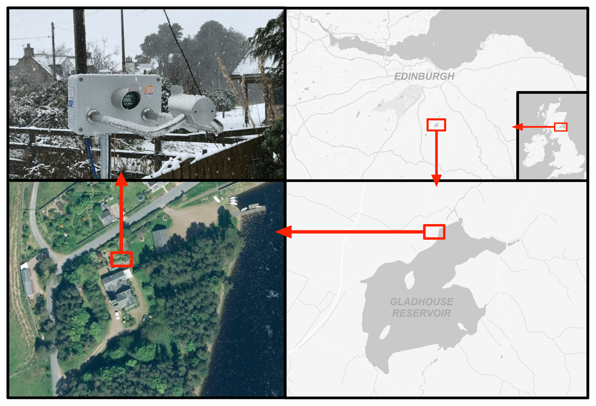
Figure 7 Maps, satellite images, and ground images of the disdrometer location and setup for winter storm Doris at Gladhouse Reservoir House, Scotland. Map data © 2018 GeoBasis-DE/BKE (© 2009), Google. Satellite image: copyright © 2012–2016 Apple Inc. All rights reserved.

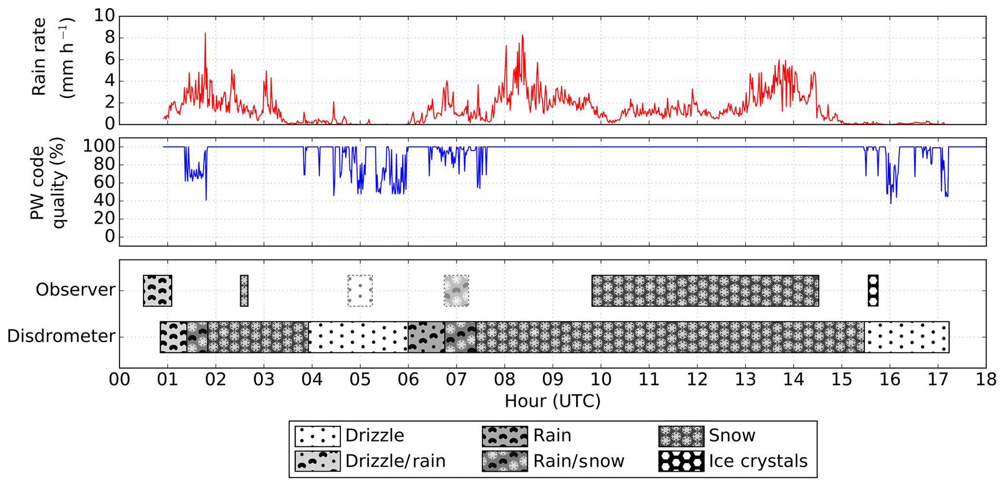
Figure 8 Rain rate, hydrometeor type, and present weather code quality index during the storm Doris event on 23 February 2017, which occurred over approximately 16 h at Gladhouse Reservoir, Scotland. Rain rate is liquid equivalent for periods of snow and is recorded by a Thies LPM disdrometer. Hydrometeor type is shown from both the disdrometer and impromptu from a trained meteorologist. The meteorologist observations at 05:00 and 07:00 UTC are approximate due to a lack of accurate time information. The disdrometer misidentified individual ice crystals at 15:39 as drizzle.

4.1 Rain–snow transition

During the first disdrometer installation trip in February 2017, the Met Office-named winter storm Doris impacted the UK. The disdrometer at Lancaster was installed on 22 February, and Edinburgh was scheduled for installation on 24 February. Storm Doris was forecast to bring heavy snowfall to the central belt of Scotland on the morning of 23 February. Therefore a decision was made to leave Lancaster early on the evening of 22 February, to arrive in Gladhouse Reservoir before the expected snowfall. An opportunity arose to temporarily operate a disdrometer at Gladhouse Reservoir (55.7776, −3.1173). Observations began at 01:00 UTC, by which time light rain had begun precipitating.

Table 4 Present weather code evolution throughout the named winter storm Doris event on 23 February 2017. All times in UTC.

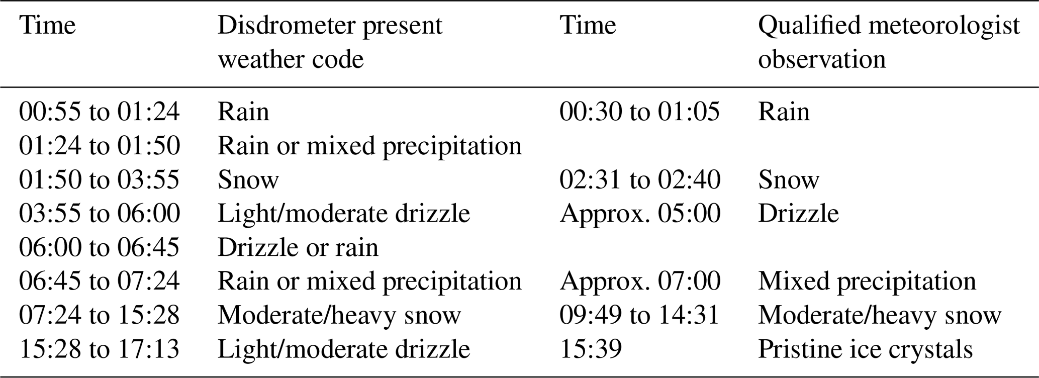
Figure 9 Accumulated particle information for each hydrometeor class period described in Fig. 8. The centre grid shows particle counts binned by size and fall velocity. The y-axis histogram shows particle velocity distribution (DVD) and the x-axis histogram shows particle size distribution (DSD) for the time period described. Since the time periods between each subplot are inconsistent in length, the colour scale and histograms have been normalized for the total precipitation over each period. The periods are as follows: (a) 00:55–01:24 UTC (rain), (b) 01:24–01:50 (rain/snow), (c) 01:50–03:55 (snow), and (d) 03:55–06:00 (drizzle).

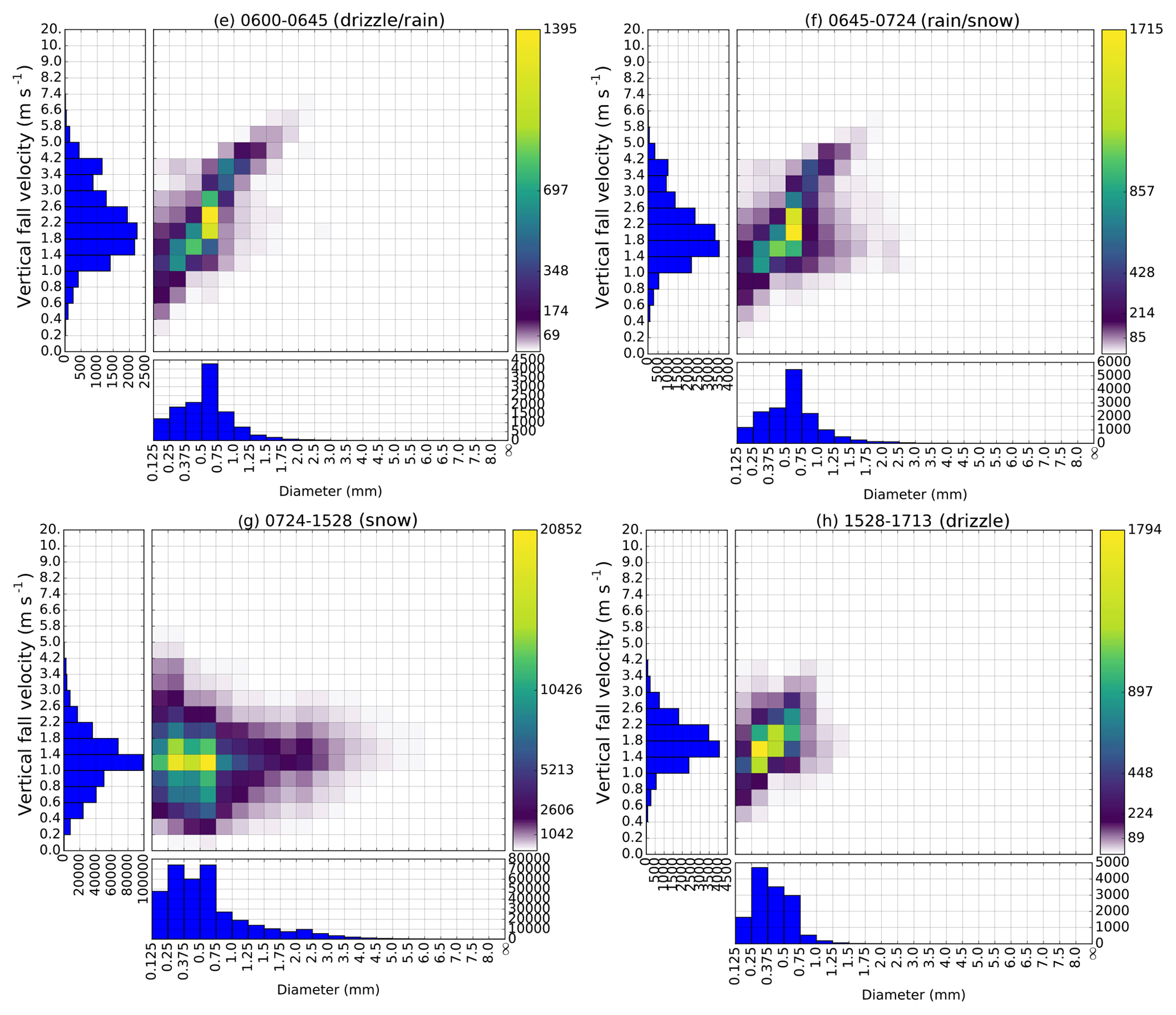
Figure 10 As in Fig. 9, but time periods are as follows: (e) 06:00–06:45 (drizzle/rain), (f) 06:45–07:24 (rain/snow), (g) 07:24–15:28 (snow), and (h) 15:28–17:13 (drizzle).

The opportunistic observations made during storm Doris provide a unique dataset by which to evaluate the skill of the disdrometer for prescribing hydrometeor type. Several transitions between rain and snow occurred that were also observed by a qualified meteorologist. The following section compares the disdrometer present weather codes and the eyewitness observations taken by the lead author during the event. An important consideration is the fact that the disdrometer was set up in a suboptimal observing environment, which had approximately 200^∘ of tall objects in close proximity. Figure 7 shows the instrument operating at Gladhouse Reservoir. There were tall evergreen trees to the east and west and a two-floor building to the south. Telecom cables were also overhead and associated poles are visible to the NNE behind the disdrometer in Fig. 7. This was unavoidable given the impromptu circumstances of deployment.

Despite the suboptimal observing conditions, the disdrometer performed well at diagnosing the correct present weather code during the storm Doris event. Table 4 and Fig. 8 show that the disdrometer correctly output a present weather code of rain initially, followed by an unverified “mixed precipitation” from 01:24 to 01:50 UTC. From 01:50 onwards a consistent snowfall present weather (PW) code was observed, which agrees with visible observations made within 01:50–03:55. At 03:55 the precipitation became light and was described as drizzle by the disdrometer.

From 06:00 onwards the precipitation intensified and the present weather code changed between drizzle and rain. By 06:45 the PW code was switching between only rain and a rain–snow mix. From 07:24 onwards the present weather code was constant snow, which continued with varying intensity until 15:28. The eyewitness observation at 15:39 is of individual ice crystals, which the disdrometer perceived as low precipitation rates of 0.293 mm h⁻¹ misclassified as drizzle. Weak precipitation continued until 17:13 where no precipitation is observed by the disdrometer, concluding the IOP.

Table 4 shows that the Thies LPM has good skill with regard to determining the present weather type. Every disdrometer-diagnosed present weather code is in agreement with the eyewitness observations throughout the IOP, with the exception of 15:39. The difference in fall velocity between drizzle particles and individual ice crystals is small and as such the disdrometer struggled to identify the precipitation correctly.

Figures 9 and 10 show the periods of constant hydrometeor type observed by the disdrometer in Fig. 8, normalized for particle count. There are clear differences between rain, snow, and rain–snow mix periods. Rain follows the curve shown by Gunn and Kinzer (1949). The rain–snow mix periods in (b) and (f) retain the Gunn–Kinzer relationship but with additional, larger particles with slower fall velocities. The snow categories in (c) and (g) are markedly different with broader distributions of particle size and a shifted fall velocity distribution. The drizzle and ice crystal periods, however, are very similar. Both are characterized by distributions of particle fall speed and diameter peaking at approximately 1.4 m s⁻¹ and 0.375 mm respectively. The distribution similarities of drizzle and pristine ice crystals in Figs. 9 and 10 illustrate the difficulty in distinguishing between these two types by fall speed and diameter alone, without additional information. A temperature sensor added to the disdrometer may have aided the PW code classification. The misidentification described here is not a major concern since pristine ice crystal precipitation is (a) uncommon in the UK and (b) contributes negligible amounts to total rainfall as indicated during this event.

The present weather code quality index shown in Fig. 8 demonstrates that the Thies LPM is able to detect when recording conditions are challenging. The PW code quality index decreases, showing a poor quality measurement, during times of weak precipitation rates and in mixed precipitation phases.

The opportunistic data collected in the storm Doris event are unusual in their number of transitional periods and will be a valuable case by which to compare the performance of radar-derived surface hydrometeor classification schemes.

4.2 Intense convective rainfall

Storm Doris also brought an interesting event to another site; a high rainfall rate observed by the NFARR Atmospheric Observatory pair of disdrometers (Chilbolton 1 & 2). The event was synoptically characterized by a narrow swath of intense precipitation oriented meridionally. The high-intensity precipitation moved west to east across the UK, associated with a cold front originating from the low associated with winter storm Doris. About 30 km NE of NFARR Atmospheric Observatory in Stratfield Mortimer, a private weather station managed by Stephen Burt also observed the intense band of rainfall (Stephen Burt, personal communication, 2017). A high-resolution Lambrecht gauge (recorded resolution of 0.01 mm) on the site observed a 75.6 mm h⁻¹ rain rate over 10 s at 07:51 UTC. The 1 min rain rate at 07:51 was 54.6 mm h⁻¹ and the 5 min rain rate ending at 07:52 was 30.6 mm h⁻¹. The event was described by a trained observer as “rain quickly became heavy then torrential”.

The event was particularly outstanding from a DiVeN point of view due to the drop count measured by the Thies LPMs situated at NFARR Atmospheric Observatory, Chilbolton, which peaked at around 12 000 drops in a single minute (200 per second) at 07:39 UTC on 23 February 2017. Both disdrometers observed a similar evolution of drop count over the short 26 min rainfall event. This does not prove that the instruments are recording accurately; conversely it may be a signal of a systematic issue with the measurement technique used in every Thies LPM.

Figure 11 shows an anomalously large left-tailed DSD from both of the Thies LPMs when compared against the Joss-Waldvogel RD-80 and Campbell Scientific PWS100 disdrometers. A high concentration of small drop sizes suggests that splashing is occurring, where larger drops breakup on impact with either the instrument itself or the surroundings. Earlier versions of the Thies LPM did not have shields on top of the sensor, which the manufacturer acknowledged were added because of splashing issues. It is possible that at very high rainfall rates, splashed droplets are still reaching the instrument beam and are being erroneously recorded. The drop velocity distribution (DVD) from the Thies LPM is also in disagreement with the PWS100. The PWS100 uses a similar optical technique to the Thies LPM with the addition of having four vertically stacked beams versus one on the Thies LPM, which should increase the accuracy of fall velocity measurements. Furthermore, the Thies LPM categorizes the highest velocity particles into the smallest diameter particle bins, which is unphysical. Finally, the total drop count per metre is significantly higher for both of the Thies LPMs.

Figure 11 Drop characteristics of a heavy rain event at NFARR Atmospheric Observatory, Chilbolton, England, on 23 March 2017. Distributions are accumulated from 07:25 to 07:50 UTC inclusively for a 26 min summation. Panel (a) shows drop size distribution and panel (b) shows drop velocity distribution. The Joss-Waldvogel RD-80 (JWD) does not provide drop velocity information. Each instrument has been normalized for sampling area and bin widths. Total drop count is listed in the top right of each plot. Both of the Thies LPMs have a higher total drop count, as well as significantly higher counts of small and high-velocity particles compared with the PWS and JWD. The frame of the Thies LPM may be splashing droplets into the beam, leading to increased counts of small, fast-moving droplets.

The DVD during the event is very wide. A noteworthy observation from the Stratfield Mortimer observatory is the wind characteristics. Marking the passage of the cold front at 07:45, winds became increasingly gusty and 10 min wind mean ending at 07:40 was 20 knots. A strong surface wind is associated with turbulent eddies, which have some vertical component. The intermittent vertical wind acts to widen the drop velocity distribution. Furthermore, turbulence breaks up droplets, thus skewing the drop size distribution. Finally, winds tangent to the beam (N–S-oriented beam, westerly wind as was the case here) increase the number of beam-edge hits, which reduce the quality of the data.

Figure 12 shows that the two Thies LPMs have good agreement for rain rate from 07:25 to 07:35 where the rain rates are moderate, but that the Thies LPMs overestimate the rainfall from 07:35 to 07:40 where the rain rate is heavy. In total, Chilbolton 1 and Chilbolton 2 recorded 120 % and 149 % of the rainfall measured by the PWS100. The JWD is expected to underestimate slightly due to the range of observable diameters (0.3 to 5 mm) being smaller than true raindrop sizes and smaller drop sizes being undetectable in the presence of large droplets due to sensor oscillation.

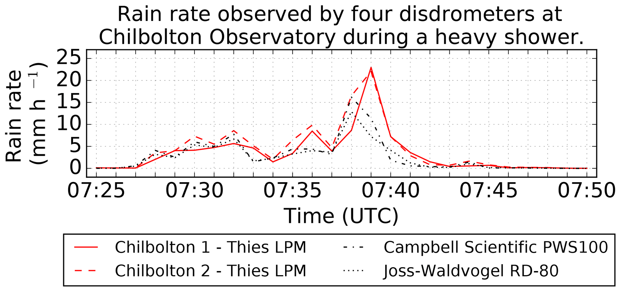
Figure 12 Rain rate measured by four instruments during a heavy rain event at NFARR Atmospheric Observatory, Chilbolton, England, on 23 March 2017. The total accumulated rain depth over the 26 min for each instrument is as follows: Chilbolton 1 (1.481 mm); Chilbolton 2 (1.847 mm); PWS100 (1.237 mm); JWD (1.090 mm). Each instrument has been normalized for sampling area and bin widths. Both of the Thies LPMs have a higher total rain rate than the PWS100 and JWD. The difference in rain rate between both of the Thies LPMs and the PWS100 and JWD is greatest during the most intense precipitation, which may be evidence of droplets splashing from the instrument housing into the measuring beam.

It appears that in these conditions the hydrometeors were not correctly measured by the Thies LPM. However, the hydrometeor type is still correctly identified despite these shortcomings in rain rate, particle diameter, and particle velocity.

4.3 Graupel shower

Graupel (rimed ice crystals) is an important signature of convection for the UK, where hail is relatively uncommon. The Thies instrument does not have a graupel category because the category does not exist within the WMO Table 4680, which it uses to convey hydrometeor type. Codes 74, 75, and 76 (light/moderate/heavy soft hail/ice grains) are presumed to be equivalent to what is commonly described as graupel.

On 25 April 2017 a shower containing conical-shaped graupel passed over Reading University “between 16:30 and 16:45 UTC” as observed by Chris Westbrook (Chris Westbrook, personal communication, 2017). Figure 13 shows the temporal evolution of hydrometeor type identified by the DiVeN instrument during the event. The disdrometer observed only a single minute (16:36) of “soft hail/ice grains” PW code (indicating graupel) during the entire 21 min of precipitation detected. Between 16:30 and 16:50 UTC inclusively, the following codes were also observed: 7 min of code 68 (moderate/heavy rain and/or drizzle with snow), 12 min of codes 61/62 (light/moderate rain), and 1 min of code 72 (moderate snowfall). Clearly the instrument struggled to diagnose graupel in this particular event.

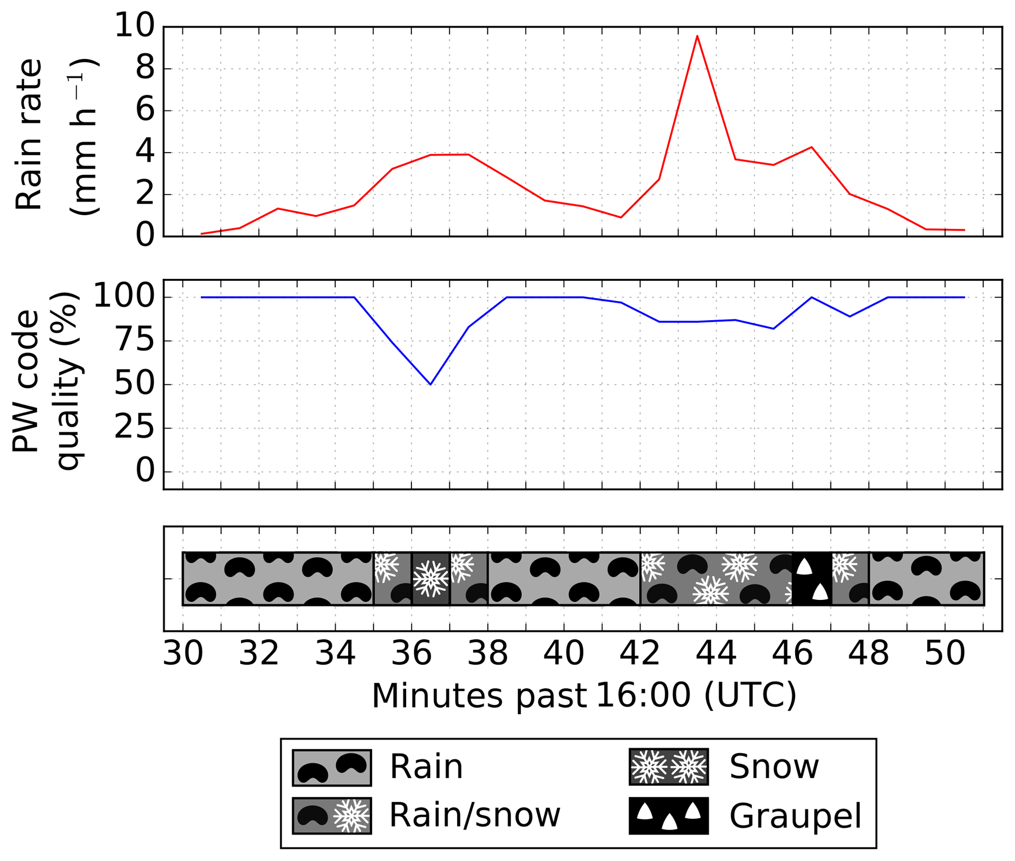
Figure 13 Rain rate, present weather code quality index, and hydrometeor type during a graupel shower in Reading, England, on 25 April 2017. The event was recorded by a Thies LPM at the Reading University Atmospheric Observatory. Conical graupel was also observed from a nearby building (approximately 500 m away) by a qualified meteorologist between 16:30 and 16:45 UTC. Rain rate is the liquid equivalent for periods of solid hydrometeors as recorded by a Thies LPM disdrometer. Hydrometeor type is shown based on the present weather code (WMO Table 4680) recorded by the Thies LPM. The instrument struggles to diagnose the graupel and instead outputs a present weather code of snow and mixed rain–snow precipitation.

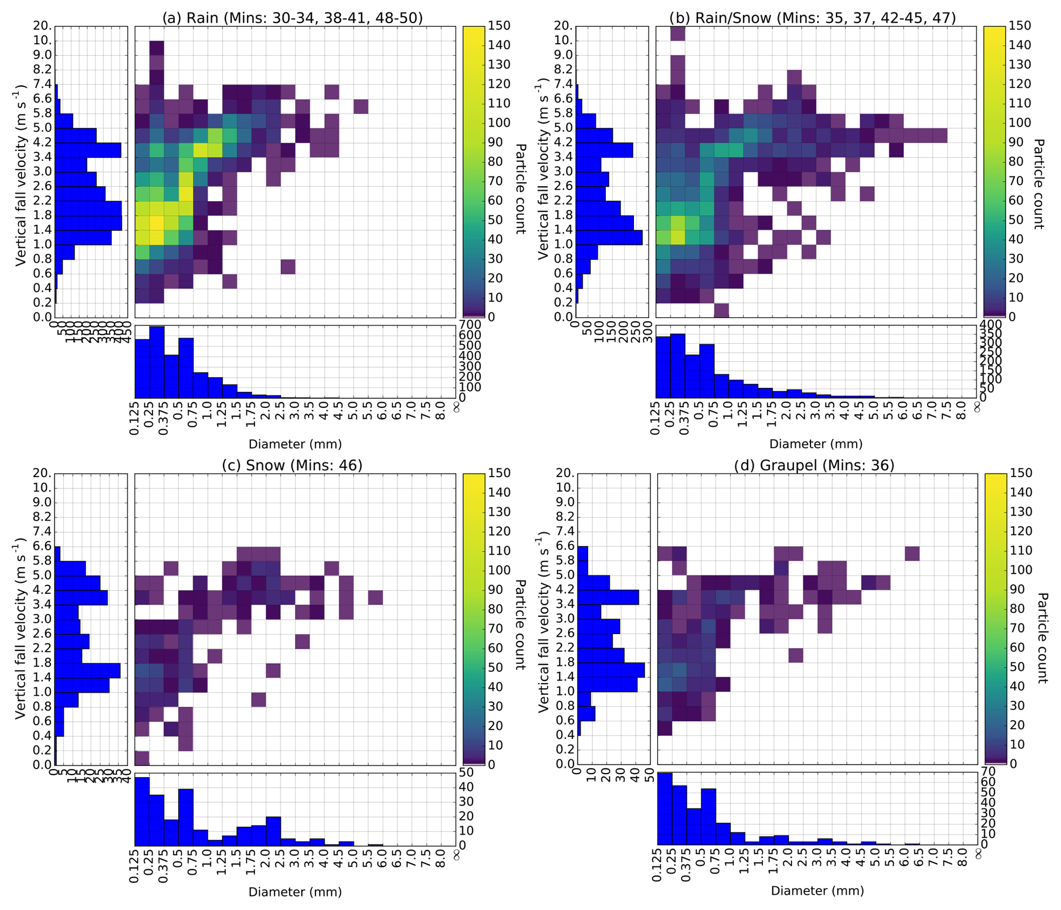
Figure 14 Accumulated particle information for each hydrometeor class period described in Fig. 13. The centre grid shows particle counts binned by size and fall velocity. The y-axis histogram shows particle velocity distribution (DVD) and the x-axis histogram shows particle size distribution (DSD) for the time period described. The periods are as follows: (a) rain (12 min), (b) rain/snow (7 min), (c) snow (1 min), and (d) graupel (1 min). The colour scale is identical in all plots despite the different time accumulations in order to highlight the rare particles.

Figure 14 shows the particle size and velocity information grouped by hydrometeor type prescribed by the Thies LPM. Throughout the graupel shower the instrument observed a bimodal distribution in both velocity and diameter for all hydrometeor types, which is indicative of both rain and graupel precipitating simultaneously. Furthermore in the rain/snow, snow, and graupel periods, a few hydrometeors exist below the Gunn–Kinzer curve, which are misidentified as snow. Although the accumulated drop characteristics for the rain and rain/snow minutes are indicative of a rain–graupel mixture, in a single minute only a few particles may fall through the disdrometer beam versus several hundred raindrops. The ratio of rain to graupel may therefore be insufficient for the PW code to change to graupel. No PW code exists in the WMO Table 4680 for a rain–graupel mixture or rain–soft hail mixture. The false detection of snow hydrometeors may be attributed to graupel particles bouncing off nearby surfaces or the instrument itself, slowing the fall velocity and thus appearing to the disdrometer as a lower-density particle such as an ice aggregate.

For future work with DiVeN data it is important to note 1 min observations of “soft hail/ice grain” PW codes when longer time periods are being analysed. For example, radar hydrometeor classification will be performed with DiVeN data at 5 min intervals. If in one of the 5 min soft hail or snow grains is observed, this must be highlighted. Graupel likely existed for longer than 1 min but it was either not the dominant hydrometeor or the instrument was unable to correctly identify it.

5 Summary

The Disdrometer Verification Network is the largest network of laser precipitation measurements in the UK. Here we have fully described the network and discussed three specific observation cases to subjectively discuss the accuracy of the Thies LPM with a focus on hydrometeor type diagnosis.

In summary, the instruments are able to correctly identify changes between snow and rain during storm Doris even with the suboptimal observing conditions. Snow is easily detected by the disdrometer and it is also able to accurately signal a mixture of hydrometeor types when transitioning between rain and snow.

Yet, the Thies LPM appears to have difficulty with measuring heavy rainfall events, where droplet breakup may be occurring due to instrument design. Distributions of drop size are skewed, such that small particle counts are significantly enhanced when compared with the Joss-Waldvogel RD-80 and the Campbell Scientific PWS100. The hydrometeor type variable was unaffected by the distribution discrepancies in the case studied.

The Thies LPM also struggled to detect graupel in the event studied here. This shortcoming can be somewhat compensated for by flagging individual minutes of present weather codes 74, 75, and 76 within larger datasets but there will be graupel cases that the Thies LPM fails to detect entirely.

A factor affecting the Thies LPM for hydrometeor classification is that empirical relationships do not account for instrument errors or the design of the instrument, which may interfere with the precipitation being measured. The hydrometeor type signatures should be derived using data from the instrument to which they will be applied. Furthermore, by using the present weather code to describe hydrometeor type, the Thies LPM is restricted in its ability to express the true nature of the observations being made, particularly noted in instances of graupel.

DiVeN offers open-access data in near-real time at 5 min updates. The 1 min frequency data are available upon request from the authors or via the Centre for Environmental Data Analysis (CEDA) from 2020. Data have been made publicly accessible in the hope that the Disdrometer Verification Network will be used for research beyond the original scope of the network.