the Creative Commons Attribution 4.0 License.
the Creative Commons Attribution 4.0 License.
 | 08 Nov 2019
Determination of ice water content (IWC) in tropical convective clouds from X-band dual-polarization airborne radar
Cuong M. Nguyen
Mengistu Wolde
Alexei Korolev
This paper presents a methodology for ice water content (IWC) retrieval from a dual-polarization side-looking X-band airborne radar. Measured IWC from aircraft in situ probes is weighted by a function of the radar differential reflectivity (Zdr) to reduce the effects of ice crystal shape and orientation on the variation in IWC – specific differential phase (Kdp) joint distribution. A theoretical study indicates that the proposed method, which does not require a knowledge of the particle size distribution (PSD) and number density of ice crystals, is suitable for high-ice-water-content (HIWC) regions in tropical convective clouds. Using datasets collected during the High Altitude Ice Crystals – High Ice Water Content (HAIC-HIWC) international field campaign in Cayenne, French Guiana (2015), it is shown that the proposed method improves the estimation bias by 35 % and increases the correlation by 4 % on average, compared to the method using specific differential phase (Kdp) alone.
- Article
(1758 KB) - Full-text XML
- BibTeX
- EndNote


Ice water content (IWC) and its spatial distribution inside clouds are known for the significant effects they exert on the Earth's energy budget and hydrological cycle (e.g. Stocker et al., 2013). Aside from its significant effect on the atmospheric processes, high ice water content (IWC >1 g m−3), which is resultant from a high concentration of small ice crystals in tropical mesoscale convective systems, has been linked to aircraft incidents and accidents (Lawson et al., 1998; Mason et al., 2006; Grzych and Mason, 2010; Strapp et al., 2016). Since early 1990s, over 150 engine rollback and power-loss events have been attributed to the ingestion of ice particles produced in convective clouds (Grzych and Mason, 2010). Many studies have been undertaken to understand the details of the meteorological processes responsible for producing areas of HIWC. Equally important, methods using multiplatform observations from ground, airborne, and space supplemented by weather models are being developed for improving detection and avoidance of high-IWC regions that would be potentially hazardous for aviation (Strapp et al., 2016).
Conventional methods of deducing IWC from radar measurements assume a statistical relationship between the radar reflectivity factor (Z) and IWC. Such relationships are usually obtained based on IWC and Z calculated from in situ measurements of particle size distributions (PSDs) and a size-to-mass parameterization (m(D)) (e.g. Heymsfield, 1977; Hogan et al., 2006). In recent studies (Protat et al., 2016), IWC was measured directly by bulk microphysical probes and Z was measured from either an airborne or ground-based radar. However, all of these studies show large uncertainties in the IWC–Z relationship despite the introduction of additional constraints such as air temperature (T) or the inclusion of refined m(D) in the IWC calculations (Fontaine et al., 2014; Protat et al., 2016).
Lu et al. (2015) conducted an extensive simulation on both millimetre- and centimetre-wavelength radar and concluded that the IWC–Z relationship is very sensitive to ice crystal PSDs (from 1 to 2 orders of magnitude in variability) and as such is not recommended for IWC retrievals. Another approach employs polarimetric observations. The non-spherical geometry of ice crystals provides information on the types and habits of ice crystals (Matrosov et al., 1996; Wolde and Vali, 2001). It has been shown that the radar-specific differential phase (Kdp) is less dependent on PSD; hence, it is potentially useful for IWC retrieval (Vivekanandan et al., 1994; Lu et al., 2015). Aydin and Tang (1997) suggested the possibility of combining Kdp and differential reflectivity ratio (Zdr) for IWC estimation for clouds composed of pristine ice crystals. However, even for the polarimetric approach, knowledge about ice crystal mass density (ρ) and axis ratio is still needed to obtain accurate estimates of IWC. Simulation results (Lu et al., 2015) show that if only the general type of ice crystals is known, errors in IWC retrieval based on Kdp are within 30 % of their true values. Unfortunately, the aforementioned parameters (ρ and particle axis ratio) are, in general, unknown and additional assumptions are often invoked. Ryzhkov et al. (1998), for instance, took into consideration ice crystal shapes and size–density parameterization of scatterers to reduce the uncertainty in IWC estimates. Modelling work (Ryzhkov et al., 1998) shows that for average-sized pristine and moderately aggregated ice crystals, the ratio between the reflectivity difference and Kdp is practically insensitive to the shape and density of the ice particles and is a good estimator of their mass.
In this paper we present a new method for assessment of IWC based on the Kdp and Zdr measurements from a side-looking X-band airborne radar in tropical mesoscale convective systems (MCSs). The IWC will be weighted with a function of Zdr to minimize the dependency of the IWC–Kdp relationship on the particle shape and orientation, hence improving the IWC estimation errors without knowledge of the PSD or density of the ice particles. The proposed method is examined using datasets collected during the High Altitude Ice Crystal – High Ice Water Content (HAIC-HIWC) international field campaign in Cayenne, French Guiana, in May 2015. The campaign was carried out to enhance the knowledge of microphysical properties of high-altitude ice crystals and mechanisms of their formation in deep tropical convective systems in order to address aviation safety issues related to engine icing (Strapp et al., 2016).
2.1 Polarimetric parameters characterizing ice crystals
In conventional single-polarization Doppler radar, measured radar reflectivity and radial velocity are used to assess cloud and precipitation spatial variability, precipitation rate, and characteristic hydrometeor types. In dual-polarization radar systems, measurements are made at more than one polarization state (Bringi and Chandrasekar, 2001). Such systems can be configured in several ways depending on the measurement goals and the choice of orthogonal polarization states. In this study, the results and discussions will be limited to the consideration of the linear horizontal and vertical (H∕V) polarization basis. The intrinsic backscattering properties of the hydrometeors for the two polarization states enable the characterization of microphysical properties such as size, shape, and spatial orientation of the cloud/precipitation particles in the radar resolution volume. Hence, using polarization, it is generally possible to achieve more accurate classification of hydrometeor types and estimate hydrometeor amounts such as rainfall rate. Polarimetric backscattering properties of hydrometeors depend on many factors such as radar wavelength, radar elevation angle, particle size, shape, orientation, etc. In this section, we summarize how the differential reflectivity (Zdr, dB) and the specific differential phase (Kdp, ∘ km−1) are measured by a polarimetric Doppler radar in the Rayleigh scattering regime and at low radar elevation angles.
In general, the differential reflectivity of an ensemble of n particles of size D and axis ratio r is given by Eq. (1) (Eq. 7.4 in Bringi and Chandrasekar, 2001),
where Shh and Svv are the diagonal elements of the backscattering matrices in the forward-scatter alignment (FSA) convention.
The specific differential phase is defined as (Eq. 7.6 in Bringi and Chandrasekar, 2001)
where n is the number concentration in reciprocal litres, k is wavenumber in reciprocal metres, Re[] stands for the real part of a complex number, and fhh and fvv are the forward-scattering amplitudes in m at horizontal and vertical polarization, respectively. Equation (2) shows that Zdr does not change with increasing number of ice particles while Kdp is proportional to n. Consequently, for a large number of small particles with the axis ratio close to unity (r≈1), Zdr→0 dB and the second term in Eq. (2) becomes small but Kdp can still be large.
In a simple form of the calculations of Zdr and Kdp of ice crystals, it is customary to approximate columns as homogeneous prolate spheroids and plates as homogeneous oblate spheroids. In the case of side incidence, the elevation angle is assumed to be close to zero and there is no (or very small) canting in the vertical plane. In the absence of wind shear and turbulence, and assuming a perfectly aligned spheroid model, Zdr and Kdp can be expressed as functions of ice particle size, axis ratio, and the relative permittivity of the particle (ε). For example, for oblate spheroid ice particles with a particle size distribution, N(D) (Eq. 7.5–7.8 in Bringi and Chandrasekar, 2001),
where Kp is dielectric factor of water at 0 ∘C (); V(D) is the particle volume; λo is the depolarizing factor, which is only a function of the axis ratio (for oblate particles; a is the semi-major axis length; and b is the semi-minor axis length (a>b)). The depolarizing factor is defined as
A similar equation for Kdp can also be derived for prolate spheroid ice particles with symmetry axis parallel to the horizontal plane (Hogan et al., 2006).
On the other hand, the IWC can be defined in terms of the size distribution,
where ρ(D) is the mass density of ice crystals with size D.
2.2 Polarimetric methods for IWC retrieval
An inspection of Eqs. (3) and (4) suggests that for small ice crystal particles, the radar cross section () is roughly proportional to the square of the ice particle mass (), a conclusion also confirmed by results from simulated data (Lu et al., 2015). In addition, according to Lu et al. (2015), for particles with sizes comparable to or larger than the radar wavelength, there is no clear relationship between the radar cross section and ice particle mass due to the Mie resonance effects. In either case, σhh,vv is not directly proportional to the particle mass. Hence, the Z–IWC relationship depends strongly on the particle size distribution and the radar frequency. Consequently, using Z only to estimate IWC without knowledge of the PSD can lead to errors as large as 1 order of magnitude. On the other hand, Eq. (6) indicates that if the terms in square brackets (α) are proportional to the ice density (ρ(D)), then the Kdp–IWC relationship is independent of PSD. The proportionality constant depends on several factors such as the ice crystal type, orientation, and the measurement elevation angle. It is shown that the variability of this proportionality constant significantly increases at large elevation angles (Lu et al., 2015). Furthermore, when the exact ice crystal type is known, averaged relative error in the estimated IWC using Kdp can be as small as 10 %, regardless of whether PSD is known or not. If the ice crystal types are unknown but can be generally categorized, the errors can be higher, but mostly less than 30 %. These numbers were averaged from elevations in the interval [0–70∘]. If IWC is estimated using Kdp at small elevation angles (less than 10∘) such as from a side-looking antenna, we would expect better results.
For a given radar volume, if the orientation of the ice crystal changes, the Kdp value changes (Eq. 7) while the IWC of the radar volume does not. Consequently, in the case of spatial variability of ice crystal shapes and orientations, the IWC estimation based solely on Kdp may be biased. To mitigate this problem, the measured IWC needs to be modified to include the information of the ice particles' orientation. One way to do this is to weight the measured IWC by a function of ice crystal shapes and orientations before applying a linear regression model to the Kdp–IWC relationship. In a simple approach, the weighting function can be in a form of (ZDR is the linear version of Zdr and a is a constant coefficient) as suggested in Aydin and Tang (1997) (derived from their approximation IWC , where a and b are constant coefficients). Proceeding more rigorously, Ryzhkov et al. (1998, 2018) demonstrated that both Kdp and difference reflectivity ZDP () are dependent on the particles' aspect ratios and orientation, whereas their ratio is very robust with respect to those factors. Indeed, in simulation and modelling work considering 12 different crystal habits, Ryzhkov et al. (2018) showed that the ratio ZDP∕Kdp in combination with reflectivity can be used to estimate IWC. In detail, for exponential size distribution and with an assumption of , β≈1, is proportional to Kdp. Also, according to Ryzhkov et al. (2018), this approximation is almost insensitive to the ice habit, aspect ratio, and orientation of the ice particles, but is affected by the degree of riming. Hence, it works better for clouds with a low degree of riming. This condition might not be true for all types of ice clouds, but might be suitable for HIWC regions, which are often composed of a high concentration of small ice particles (Leroy et al., 2016).
At ZDR≈1 (or Zdr≈0 dB), the weighting function is close to zero, and hence it can introduce large errors in the estimates. Therefore, there should be a certain threshold for Zdr to determine how the weighting function would be calculated. In detail, if Zdr is less than a threshold, the weighting function is replaced by . In this paper, we use ZDR-threshold=1.12 (see Sect. 6 for more detailed derivation of this threshold value). This threshold is very close to a 1.15 threshold proposed by Ryzhkov et al. (1998) for “cold” storms for temperatures below −5 ∘C.
In summary, there are two polarimetric methods for IWC retrieval, which will be investigated and compared in this paper. They are expressed as
where model parameters (ai,bi) will be estimated from measured data. A flow chart of IWC retrieval using Kdp and ZDR is shown in Fig. 1.
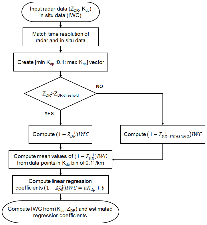
Figure 1Flow chart of IWC retrieval using (Kdp,ZDR) and in situ data. In this paper, ZDR-threshold=1.12.
During the Cayenne HAIC-HIWC project, the NRC Convair CV-580 conducted 14 research flights in both continental and oceanic mesoscale convective systems (MCSs) with high IWC. All the flights were conducted during daytime only due to flight restrictions. Analysis of all the IR satellite imageries show that the Convair flights were performed close to the peak intensities of the targeted MCSs, which had a typical lifetime of 7.5 and 4.5 h for oceanic and continental MCSs, respectively (Walter Strapp, personal communication, 2019). So the fact that the flights were conducted only during the daytime did not prevent the flights from sampling of the storms during their peak intensities. For this campaign, the Convair aircraft was instrumented by the NRC and Environment and Climate Change Canada with an array of in situ cloud microphysics probes, atmospheric sensors, and the NRC airborne W- and X-band (NAWX) Doppler dual-polarization radars (Wolde and Pazmany, 2005). The unique quasi-collocated in situ and radar data collected during the HAIC-HIWC mission provided a means for developing techniques for detection and estimation of high IWC that could be adopted in operational airborne weather radars.
3.1 Airborne radar data
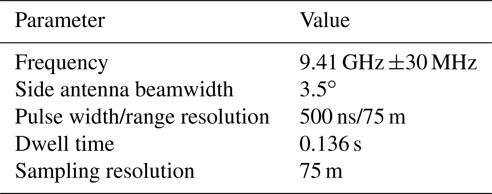
In this study, dual-polarization radar data from the NRC airborne X-band radar (NAX) (Fig. 2) side-looking antenna are used. Some important radar parameters are given in Table 1. More detailed information on the radar system can be found in Wolde and Pazmany (2005). In the Cayenne project, the radar complex I and Q samples are processed to powers and complex pulse pair products according to the radar parameter specification table, and the products are recorded in binary format. Due to the size of the aircraft radar radome, the NAX dual-polarization parabolic side antenna is relatively small (0.66 m), hence exhibiting some limitations in terms of side lobe performance. The antenna orthomode transducer (OMT)–feedhorn combination is relatively large compared to the parabolic dish. The large feed structure creates some significant side lobes at ±90∘ planes. As a result, when the side lobes intercept targets with strong returns below the aircraft, such as the earth surface or a storm melting layer, significant returns from the side lobes will contaminate signals coming via the antenna's main lobe. In most situations, the effect is more prominent at a range equal to or greater than the distance where the antenna side lobes hit the ground. At regions where signals are contaminated by ground clutter via the side lobes, the data are intermittent and exhibit large biases. Unfortunately, with the pulse pair data from the Cayenne campaign, methods to separate clutter from the precipitation signals are limited. To overcome this issue, a method is developed to detect regions with strong clutter contamination based on signal correlations between the nadir and zenith returns. If the correlation coefficient exceeds a predefined threshold, the corresponding side data in those regions are discarded. If the width of the discarded data region is relatively small (less than 300 m in radar range) it will be filled through interpolation. In addition, due to the limitation of the radar hardware, the measurements of dual-polarization parameters are not useable below a range of 1000 m from the aircraft, but reflectivity can be measured accurately from 450 m. Hence, in this work, radar profiles were extracted at a horizontal distance of 1000 m from the aircraft. This is not an ideal condition when the in situ data and the radar data are not spatially coincident. However, in most scenarios the advantage of having fine radar sampling volumes with a high order of accuracy in time synchronization between in situ probes overcomes the location offset. At large distances from cloud boundaries and convective cores, the microphysics properties of glaciated clouds can be considered spatially quasi-uniform at scales of the order of a few hundred metres. This is specifically relevant to the measurements in MCSs during the HAIC-HIWC project. Moreover, there was no attenuation correction applied to reflectivity and Zdr because in ice precipitation regions and at close range attenuation at the X-band is negligible.

For the Cayenne project, the in situ microphysical data are processed at 1 Hz, which is lower than that of the radar data. Hence, the radar data were decimated to match with temporal resolution of the in situ data. At the Convair CV-580 average ground speed of 100 ms−1, this results in a 100 m radar sampling volume.
3.2 In situ data
For the project, the NRC Convair CV-580 was equipped with state-of-the-art in situ sensors for measurements of aircraft and atmospheric state parameters and cloud microphysics. There were multiple sensors to measure bulk liquid water content (LWC) and total water content (TWC), with hydrometeor size distribution ranging from small cloud drops to large precipitation particles. A detailed list of the Convair in situ sensors used during the Cayenne HIWC-HIWC project is provided in Wolde et al. (2016). Here we will briefly describe the in situ microphysical sensors used in correlating the airborne radar measurements with regions of HIWC. TWC was measured by an Isokinetic probe (IKP2) that was specifically designed to measure very high TWC (Davison et al., 2008). Alternatively, IWC was estimated from the measured PSDs with the D–M parameterization tuned using IKP2 measurements. In the Cayenne Convair datasets, IWCs calculated from PSDs and measured by IKP2 agreed quite well and the difference between them in the HIWC regions on average did not exceed 15 %. Because the IKP2 data were not available in all flights, estimated IWC from PSDs (IWCPSD) has been used in this work. Additionally, mean mass diameter (MMD) was also used to characterize the microphysical properties of the high-IWC regions and interpret X-band radar measurements. MMD was calculated from composite particle size distributions measured by SPEC 2D-S and DMT PIP 2-D imaging probes.
As shown in Korolev et al. (2018) in the MCSs studied during the Cayenne HAIC-HIWC project, the fraction of mixed-phase clouds at −15 ∘C ∘C did not exceed 4.6 %, and in most mixed-phase cloud regions LWC ≪ IWC. Hence, we did not filter out the very small fraction of liquid observed in our analysis; i.e. we assumed TWC = IWC. This finding significantly simplifies the processing and interpretation of cloud microphysical measurements.
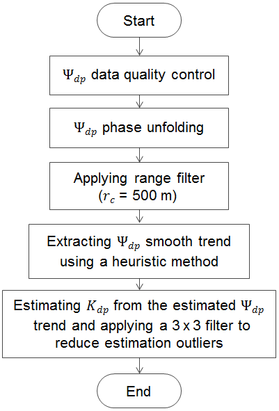
The radar specific differential phase (Kdp) is defined as the slope of the range profile of the differential propagation phase shift Φdp between horizontal and vertical polarization states (Bringi and Chandrasekar, 2001). The measured differential phase shift between the two signals at the H and V polarizations, Ψdp, contains both Φdp and differential backscatter phase shift δdp. If δdp is relatively constant or negligible, the profile of Ψdp can be used to estimate Kdp. The estimated phase Ψdp usually exhibits discontinuities due to phase wrapping, statistical fluctuations in estimation, and the gate-to-gate variation in δdp. Because the statistical fluctuations in the estimates of Ψdp will be magnified during the differentiation, resulting in a large variance of the Kdp estimates, the following considerations need to be addressed in the Kdp estimation algorithm.
Phase unfolding. Phase wrapping occurs when the total Φdp accumulation exceeds the unambiguous ranges. This depends on the system differential phase Φdp(0) and the cumulative phase due to the medium. The NAX radar operates in the simultaneous transmission mode (VHS) and the unambiguous range is 360∘. The system differential phase Φdp(0) of NAX is about 64∘. For the Cayenne dataset, no observations were made when the phase was folded.
δdp “bump”. It seems that δdp was negligible in the HIWC environment in the Cayenne campaign. We did not observe the presence of significant changes in δdp over a short range.
Range filtering. In this work, the range scale was set at 500 m; thus the fluctuations at scales smaller than 500 m will be suppressed.
Once the phase data are quality controlled, filtered, and decimated to match the temporal resolution of the in situ data, a heuristic algorithm similar to one reported in Rotemberg (1999) is applied to the data to extract the Ψdp smooth trend and then Kdp is computed from it. This approach does not require an assumption of Φdp being a monotonically increasing function as it is in some other existing Kdp retrieval algorithms (Wang and Chandrasekar, 2009); therefore, it would also work well with negative Kdp, which possibly appears in ice clouds. Our preliminary analysis shows that the algorithm can provide estimates with standard deviation no greater than 1 ∘ km−1. The NRC Kdp estimation algorithm is summarized in the flow chart below.
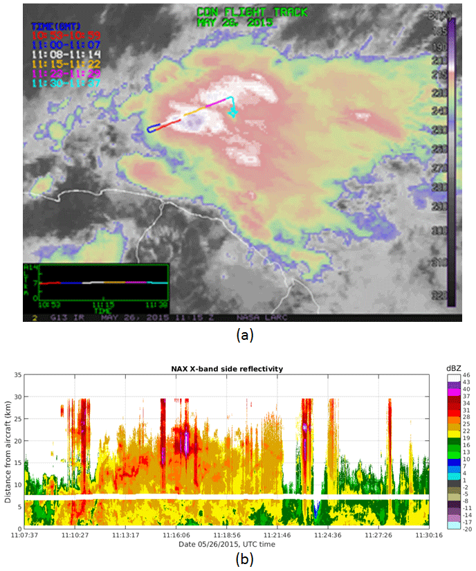
Figure 4Panel (a) shows IR GOES-13 image with the overlaid segments of the Convair CV-580 flight track on 26 May 2015. Different time segments of the flight track are shown by different colours. Panel (b) shows X-band side reflectivity from a period of 11:07–11:30 UTC corresponding to white, yellow, and purple segments in (a). A break line at around 7.1 km is the location of contaminating ground clutter via the side antenna's side lobe (Sect. 3.1), which was filtered out.

Figure 5Time series of (a) IWCPSD, MMD, (b) Kdp, Zdr, (c) ρhv, and ZH for 26 May Convair CV-580 flight.
In this section, results illustrating the performance of the proposed polarimetric algorithms are presented. In addition to the polarimetric method, we also include results from the conventional IWC–Z relations for comparison. Because the histogram of static temperature (not shown) indicated a bimodal distribution with two centres at around −5 and −10 ∘C, two IWC–Z relations at ∘C (IWC =0.257Z0.391) and at ∘C (IWC =0.253Z0.596) were obtained by fitting power-law curves to scatter plots of all the data points at those two temperature levels (Wolde et al., 2016).
5.1 Case study I: 26 May flight
In this case, a 20 min segment of the Convair flight inside an Oceanic MCS on 26 May 2105 is selected for analysis. The MCS was sampled north-northwest of Cayenne, French Guiana, during early morning hours. Figure 4a shows IR satellite imagery obtained during the flight where the aircraft's flight track is shown in different colours, which represent the aircraft's location at different time segments. The reflectivity field from the NAX side antenna is shown in Fig. 4b. The selected period begins at a point when the aircraft started to sample at the proximity of the convective core of the storm with the lowest cloud-top brightness temperature (white segment in the IR image). The brightness temperature was increasing toward the end of the segment (magenta segment). The aircraft flew between 6.9 and 7.2 km altitude and the static air temperature (Ts) varied from −12.8 to −8.2 ∘C. In addition to the radar data, IWCPSD and MMD time series from particle probes are shown in Fig. 5. The IWC estimates from radar data have been decimated to match with the temporal resolution of the in situ data.
The aircraft sampled two regions: a convective region before 11:23 UTC and a stratiform region after 11:25 UTC (Fig. 4b), with IWC in both regions mostly higher than 1.5 g m−3 (Fig. 5a). It is worth noticing that the reflectivity measurements along the flight path were fairly constant at ∼20 dBZ and the MMD values were relatively small at HIWC regions (IWC >1.5 g m−3) (Fig. 5a). From Fig. 5, it follows that (1) Kdp, in general, is highly correlated with IWC; (2) Kdp increases at the regions dominated by small ice crystals (between 11:08 to 11:16 and 11:24 to 11:27 UTC); and (3) regions with larger MMD exhibit deceasing ρhv and increasing Zdr. In Fig. 6, Zdr, ρhv, and IWC are expressed as functions of Kdp. In this case, there is a break point at Kdp≈1.5 ∘ km−1 (and ZDR∼1.12) where Zdr started increasing and ρhv decreased with respect to Kdp. At Kdp<1 ∘ km−1, Zdr was mainly flat and IWC linearly increased with respect to Kdp (Fig. 6b). This suggests the pristine ice crystals' axis ratio might be fairly constant, but the particle number density increased, resulting in an enhancement in both Kdp and IWC (shown by a linear IWC–Kdp relationship). From Kdp>1 ∘ km−1, the Zdr increment with respect to Kdp was greater, but the IWC increase does not follow the same degree as in the previous segment. If a linear IWC–Kdp relationship derived from the first segment (Kdp<1 ∘ km−1) is applied to the second portion, IWC will be overestimated. It is not easy to identify the exact reasons of this observation. Many factors could contribute to this circumstance such as changes in ice crystals' size, shape, orientation (e.g. particles with higher axis ratio that are aligned in the horizontal plane), or particle density. In this work we used Kdp and Zdr to mitigate this dependency and improve estimation of IWC. In Fig. 6b and c, measured IWC and IWC are shown as solid black lines and their linear fitting curves (red lines) are superimposed. The R2 goodness-of-fit parameter indicates that a linear regression fits IWC better in comparison to IWC.
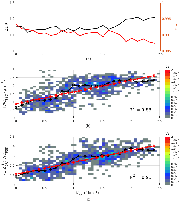
Figure 6Zdr and ρhv (a), IWCPSD (b), and (c) as functions of Kdp. In panels (b) and (c), mean values and frequency distributions are computed from data points in each Kdp bin of 0.1 and 0.05 ∘ km−1, respectively. Regression parameters (a1,b1) for the Kdp-only method and (a2,b2) for the (Kdp,ZDR) method are estimated from the mean values using a simple linear fitting algorithm.
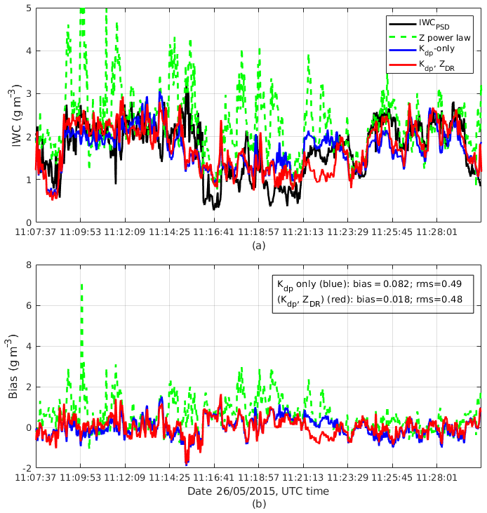
Figure 7Panel (a) shows IWCPSD (black line), estimated IWC using reflectivity (dashed green line), Kdp alone (blue line), and the (Kdp, ZDR) combination (red line) for the 26 May case. Panel (b) shows estimation biases for the three estimators. Average biases for IWC(Z), IWC(Kdp), and IWC(Kdp, ZDR) are 0.60, 0.082, and 0.018 g m−3 and rms differences are 0.98, 0.49, and 0.48 g m−3 for the three algorithms, respectively.
To gauge the performance of the polarimetric methods, results from the conventional IWC–Z estimator are also included in Fig. 7a. This figure shows the measured IWC along the Convair's flight path depicted in black, IWC–Z results in green, and IWC estimates using polarimetric methods in blue and red for Kdp-only and (Kdp, ZDR) algorithms, respectively. One can observe that the two polarimetric methods agree well with measured IWC while the IWC estimates from just using radar reflectivity exhibit biases as large as 1 order of magnitude. The large errors in the IWC–Z estimator are due to the presence of mixtures of large aggregates and small ice crystal regions as indicated in the PIP images (not shown) in clouds. Large aggregates have a dominant contribution into the radar reflectivity, which explains the positive biases of the IWC–Z estimates. On the other hand, Kdp is not biased toward large aggregates. The magnitude of Kdp in aggregates with MMD >2 mm is usually smaller than 0.4 ∘ m−1 and in small ice particles (MMD in the range 0.3–1 mm) Kdp is between 0.6 and 1 ∘ km−1 (Fig. 8a). It follows that estimators utilizing Kdp information would overcome the large aggregate effects in radar volumes. It is worth noting that the two algorithms capture the IWC variation at the end of the segment well. If the in situ measurements are considered as the ground truth, the estimation biases are computed and shown in Fig. 7b. On average, biases are 0.082 and 0.018 g m−3, and the root-mean-square differences (hereinafter referred to as the rms differences) are 0.49 and 0.48 g m−3 for the Kdp alone and (Kdp, ZDR) methods, respectively. The correlation coefficients between IWCPSD and estimated IWCs are 0.66 and 0.70 for the two methods. In this case study, the inclusion of Zdr improves the accuracy of the IWC estimates.
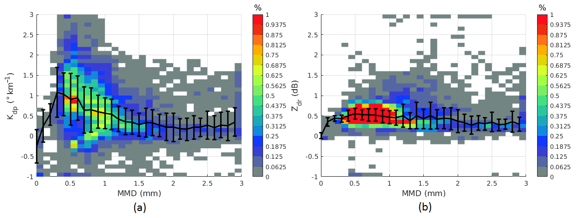
Figure 8Kdp (a) and Zdr (b) as functions of median mass diameter (MMD). Over 17 000 data points from seven selected flights (Sect. 6) during the Cayenne campaign are used.
5.2 Case study II: 23 May flight
For this case, a segment of the Convair flight on 23 May 2015 inside an MCS north of the Surinam coast and over French Guiana (Fig. 9a) is selected. The flight segment consists of a HIWC region of a very high concentration of small ice particles and a region of mixed moderately large aggregates and pristine ice crystals. This affords an excellent example to gauge the performance of the algorithms. In Fig. 9a, the selected segment is displayed in purple. The radar reflectivity field from the side antenna is shown in Fig. 9b. In this segment, the aircraft's altitude was between 6.74 and 6.78 km and Ts ranged from −11 to −8 ∘C.

Figure 9Similar to Fig. 4 but for the 23 May case.
In addition to the radar data, IWCPSD and MMD time series from particle-imaging probes are shown in Fig. 10. The aircraft sampled two small cores where IWC was higher than 1 g m−3 (∼18:30 and ∼18:34 UTC). At these high IWC cores, the clouds were dominated by small ice particles (Fig. 11a) and MMD was in the 400 µm range. In contrast, for the flight segment between 18:36 and 18:44 UTC, when the temperature was higher, the aircraft sampled a mixture of large aggregates with sizes exceeding 6 mm and small ice particles (Fig. 11b), where the IWC was less than 0.5 g m−3.
The IWC estimates from the methods are depicted in Fig. 12a. In the regions around the two HIWC peaks, results from the three estimators agree quite well with IWCPSD. There are small biases in the outcomes of the two polarimetric algorithms that can be attributed to the errors of fitting linear regression models to the data and/or the difference in the sampling locations of the radar and the in situ data (Sect. 3.1). In the region after 18:38 UTC, the IWC–Z results show very large errors due to the presence of aggregates in the clouds. The large aggregates dominate the measurements of radar reflectivity, resulting in positive biases of the IWC–Z estimates (Fig. 12b). The errors for this case are as large as 300 % in most estimates. In contrast, both the polarimetric methods provide much better results compared to the conventional IWC–Z method. They capture the variation in IWC at smaller scales (around 18:33:58 UTC) and larger scales (around 18:41:54 UTC) well. This again confirms that these algorithms are robust to the variation in ice crystal type, shape, and distribution. The rms differences and correlation coefficients for the Kdp-only and (Kdp, ZDR) methods are (0.84 g m−3, 0.41) and (0.79 g m−3, 0.55), respectively. The combination of Kdp and ZDR provides better results, which can be seen at the edges of the second IWC peak (indicated by ellipses) in Fig. 12a. At those regions, MMD (Fig. 10) and Zdr (not shown) values are large. This may be an indication of ice crystals with a high axis ratio aligned in the horizontal plane. When this happens, the algorithm based on Kdp alone will overestimate IWC. On the other hand, the product IWC already includes the particles' shape and orientation effects; thus, estimates based on it should yield better results. When large particles dominated the volume (after 18:36:14 UTC) Zdr become small (Fig. 8b), and then the (Kdp,ZDR) estimator provides no advantage over the Kdp-only estimator.
In the previous section, two case studies were analysed in detail. In both cases, results from the polarimetric methods show a much better agreement with in situ measurements compared to the IWC estimates from the radar reflectivity factor, especially when larger particles dominate the radar volume. In addition, applying a function of ZDR to IWC before fitting a linear regression model to the data improves the estimation accuracy and correlation. In this section, more data from different flights collected during the mission were analysed and summarized. Out of total 14 campaign flights, there were seven flights with good data quality (radar and in situ) and with an applicable number of high-IWC data points, and data from those flights were used this analysis.
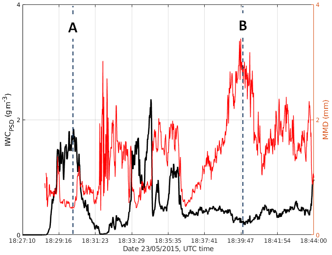

Figure 11Samples of 2-D imagery from the SPEC 2D-S (a) and DMT PIP (b) probes at two time stamps as in Fig. 10. The width of the 2D-S image strip is 1.28 mm and that of the PIP is 6.4 mm. The aircraft's altitude was 6.75 km at A and 6.74 km at B.
ZDR threshold (Sect. 2.2) is determined from all selected data (17 699 points in total). In order to find an optimal ZDR threshold from the available data, average bias and rms of IWC estimates are expressed as a function of the ZDR threshold (Fig. 13). ZDR threshold was changed within [1.01, 1.2] with 0.1 increments, and bias and rms were computed for each value of ZDR threshold. In Fig. 13, average bias and rms of IWC estimates from the Kdp-only algorithm, which are independent of ZDR threshold, are also displayed (blue lines). It follows that the average biases for the two methods are very small (within ±0.08 g m−3) and the (Kdp, ZDR) method provides unbiased estimates at a ZDR threshold of 1.06. However, rms of the (Kdp,ZDR) method is quite large at a small ZDR threshold and reduces with an increasing ZDR threshold. It becomes saturated at 0.498 g m−3, which is slightly below the rms of the Kdp-only algorithm. Considering all the factors, we selected an optimal ZDR threshold of 1.12, where rms values of the two methods are equal but the average bias is smaller with the (Kdp,ZDR) method.

Figure 12Similar to Fig. 7 but for the 23 May case. Average biases for IWC(Z), IWC(Kdp), and IWC(Kdp, ZDR) are 1, −0.189, and −0.222 g m−3 and rms differences are 1.34, 0.84, and 0.79 g m−3 for the algorithms, respectively.
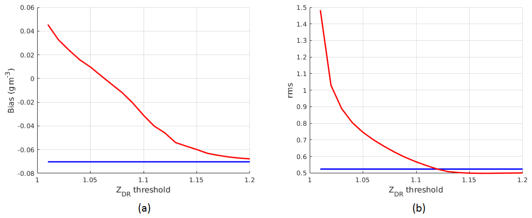
Figure 13Average bias and rms as a function of ZDR threshold for all data from the seven selected flights.
In Fig. 14, IWC and IWC are expressed as functions of Kdp for selected flights. Linear fits to all the data from selected flights are also shown. The respective y axes are scaled to the maximum value of IWC and IWC for comparison. For most cases, the linear relationships are well approximated up to Kdp=2 ∘ km−1. At larger Kdp, IWC saturates at 2.5 g m−3 and the IWC–Kdp relationship departs from the linear trend. Due to the limited amount of data of large measured Kdp and IWC, identifying the major reasons for this saturation is not attempted. In these scenarios, applying a more sophisticated method (such as a parametric model) will likely reduce errors at high Kdp, but this is beyond the scope of this paper. Here, a simple linear regression model (based on the approximation in Eq. 13) is used and errors are computed from all data points.
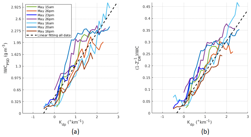
Figure 14IWCPSD (a) and (1-)IWC (b) as functions of Kdp for the seven selected flights. Linear fits (dash lines) are also plotted using coefficients computed from all data point (Table 2).
Table 2Polarimetric method performance for selected flights during the Cayenne 2015 campaign. The MCS types and scales from Strapp et al. (2016) are also listed.
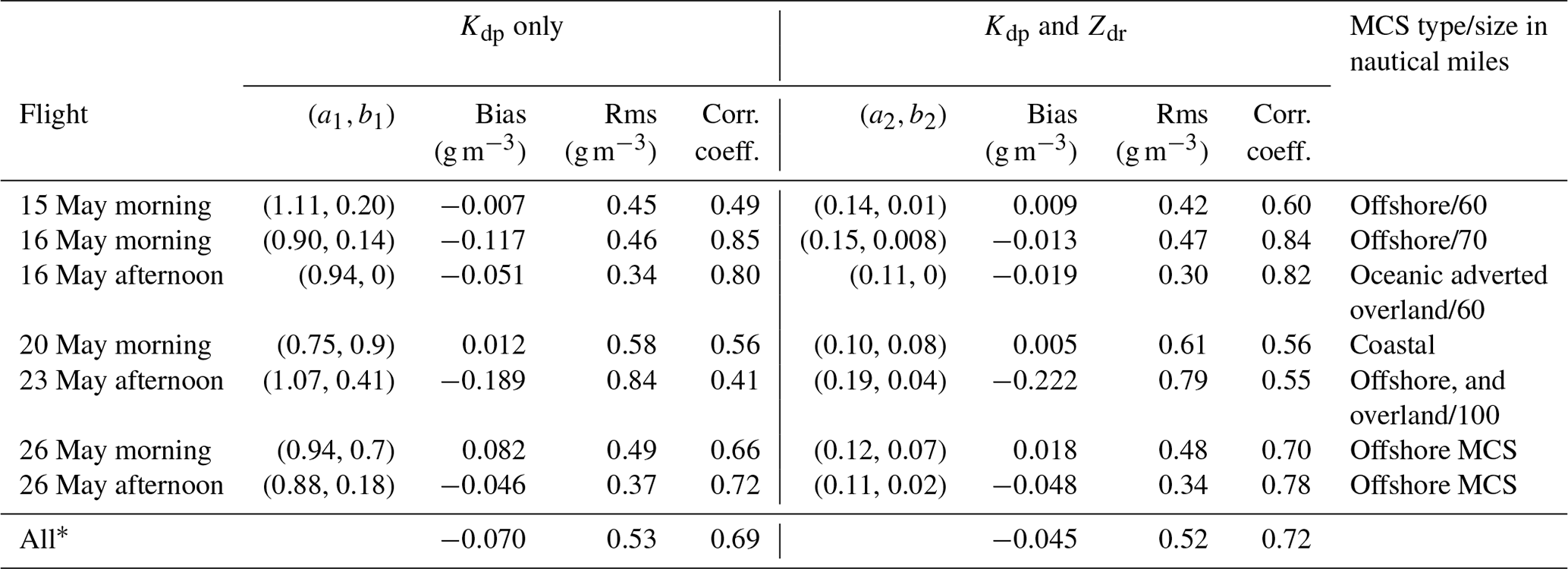
* For all data points, optimal fitting parameters (0.88, 0.45) were used for the Kdp-only algorithm and (0.13, 0.04) were used for the (Kdp, Zdr) algorithm.

Figure 15(a) Combined IWC time series data from the selected flights: measured IWC (black line), estimated IWC using Kdp alone (blue line), and estimated IWC using Kdp and ZDR (red line). (b) Estimation errors for the two estimators. For all study cases, the aircraft flew in the range of [5.6, 7.5] km and most of the data points were within a temperature range of (−10 ∘C ±25 ∘C).

Figure 16Bias and rms difference as a function of IWC derived from the seven selected flights. Mean values and standard deviation are computed from data points in each IWC bin of 0.2 g m−3.
It is also worth noting that the deviation of the IWC–Kdp curves from the linear fit is smaller compared to that of the original IWC–Kdp curves. This spread in the IWC–Kdp relationship can be attributed to the properties of ice crystals and the medium's state. In other words, when the dependency of the IWC–Kdp relationship on ice crystal shape and orientation was removed (or partially removed), the spread in the IWC–Kdp relationship around the linear fit should be smaller. This is a very important outcome which helps to reduce estimation errors when a single estimator is used for all the cases. Results for IWC estimates are shown in Table 2 for the two polarimetric methods only. In each row, statistical error analysis is shown for each flight with the optimal fitting model derived from data of that flight. Information about MCS of selected flights is also provided. The last row displays results computed from all selected data of 17 699 points. In all cases, improvement in IWC estimation when Zdr information is utilized in the algorithm is clear. For all data, the bias changes from −0.07 to −0.045 g m−3 and correlation coefficient increases from 0.69 to 0.72. The standard deviations of the fitting coefficients (a1,b1) for the Kdp-only method and for (a2,b2) for the (Kdp, ZDR) method are (0.12, 0.33) and (0.032, 0.033), respectively. The uncertainty of the retrieval depends on the uncertainty in the fitting parameters as well as the values of Kdp and ZDR and their measurement accuracy. Typical values of Kdp and ZDR for HIWC regions (MMD between 0.3 and 1 mm) are about 1 ∘ km−1 and 1.12 (Fig. 8). At those typical values, standard deviation of IWC estimates using the (Kdp,ZDR) algorithm is 0.6 g m−3.
Figure 15 shows time series of IWCPSD from the seven flights and estimated IWC from the two algorithms. As mentioned before, for each algorithm, a single set of fitting parameters is used for the combined data. Evidently, the method utilizing Zdr yields better results in terms of estimation bias and correlation (Table 2). In Fig. 16, estimation bias and standard deviation are expressed as a function of IWC. It can be seen that inclusion of Zdr improves estimation bias at all IWC points. On average, an improvement of 35 % in average bias was achieved. As observed in Fig. 16, larger biases happen at IWC greater than 2 g m−3. This is attributed to strong departures from the linear model in the joint IWC–Kdp distribution. The inclusion of Zdr has been proven to be able to mitigate these large errors but not completely fix the problems. To improve the radar-derived IWC estimates further, more additional data processing (such as hydrometeorology classification) and more sophisticated regression models are needed.
Accurate detection and estimation of HIWC in tropical mesoscale convective systems are critical for reducing hazards caused by the ingestion of ice particles into the engines of commercial aircraft. The objective of this paper is to find a method to improve IWC retrieval from a side-looking X-band dual-polarization airborne radar. It is shown that the use of the specific differential phase (Kdp) and differential reflectivity ratio (Zdr) significantly reduces errors in IWC retrieval over the conventional IWC–Z method. In general, the IWC–Kdp relationship can be approximated by a linear model, and IWC retrieval using Kdp captures the IWC variation very well, regardless of the information of PSD. One major drawback of the Kdp algorithm is that it provides large estimation biases when the ice particle's aspect ratio and orientation are changing. To mitigate this effect, Zdr is used to reduce the dependency of IWC on the variation in ice particles' shapes and orientation. We proposed a method in which IWCs are weighted by a function of Zdr before applying a linear model to the IWC–Kdp joint distribution. This approach uses an assumption of a low degree of riming within the radar volume. This is suitable for HIWC regions, which are often composed of a very high density of small ice particles. Zdr at regions of mixtures of small pristine ice crystals and larger particles such as aggregates is generally low and will not be used in the weighting function. Results from selected Convair CV-580 flights from the Cayenne campaign show that the proposed method is able to improve estimation biases by 35 % and correlation by 4 %, on average. In our analysis, a single set of fitting parameters is applied for all the data points. The results can be improved further by including advanced data processing techniques such as ice crystal type classification or using a more sophisticated regression model for the modified IWC–Kdp joint distribution.
Most of HIWC data points used in this are measured at a narrow window of the temperature range (−10 ∘C ±2.5 ∘C). More data are needed to study the temperature variability of the proposed method.
The data used in this analysis are stored at the National Research Council database. Please contact the lead author for access to the data.
CN developed the algorithms, processed radar data, and performed the data analysis. MW was the flight mission scientist for all the flights and operated the radar. MW, AK, and Ivan Heckman (ECCC) processed the in situ data. The paper was written by CN. MW and AK have provided content for sections of the paper and also reviewed the draft and made some changes to the original draft.
The authors declare that they have no conflict of interest.
This work is supported by the FAA (NAT-I-8417) and the NRC RAIR programme. We would like to acknowledge Jim Riley, Tom Bond, and Chris Dumont of FAA and Steve Harrah of NASA for their support for this work. We thank the engineering, scientific, and managerial staff from NRC and ECCC, who made the project possible by working long hours during instrument integration and field operations. Special thanks are due to Ivan Heckman (ECCC) for support of processing cloud microphysical data. We would also like to acknowledge the support we received from the HAIC-HIWC community during the flight campaign.
This paper was edited by Brian Kahn and reviewed by Alexander Ryzhkov and two anonymous referees.
Aydin, K. and Tang, C.: Relationships between IWC and polarimetric measurements at 94 and 220 GHz for hexagonal columns and plates, J. Atmos. Ocean. Tech., 14, 1055–1063, 1997.
Bringi, V. N. and Chandrasekar, V.: Polarimetric Doppler Weather Radar: Principles and Applications, Cambridge University Press, 636 pp., 2001.
Davison, C. R., MacLeod, J. D., Strapp, J. W., and Buttsworth, D. R.: Isokinetic Total Water Content Probe in a Naturally Aspirating Configuration: Initial Aerodynamic Design and Testing, 46th AIAA Aerospace Sciences Meeting and Exhibit, Reno, Nevada, AIAA-2008-0435, 2008.
Fontaine, E., Schwarzenboeck, A., Delanoë, J., Wobrock, W., Leroy, D., Dupuy, R., Gourbeyre, C., and Protat, A.: Constraining mass–diameter relations from hydrometeor images and cloud radar reflectivities in tropical continental and oceanic convective anvils, Atmos. Chem. Phys., 14, 11367–11392, https://doi.org/10.5194/acp-14-11367-2014, 2014.
Grzych, M. and Mason, J.: Weather conditions associated with jet engine power loss and damage due to ingestion of ice particles: What we've learned through 2009, 14th Conf. on Aviation, Range and Aerospace Meteorology, Atlanta, GA, Amer. Meteor. Soc., 6.8, 2010.
Hemsfield, A. J.: Precipitation development in stratiform ice clouds: A microphysical and dynamical study, J. Atmos. Sci., 34, 367–381, 1977.
Hogan, R. J., Mittermaier M. P., and Illingworth, A. J.: The retrieval of ice water content from radar reflectivity factor and temperature and its use in evaluating a mesoscale model, J. Appl. Meteorol. Clim., 45, 301–317, 2006.
Korolev, A., Heckman, I., and Wolde, M.: Observation of Phase Composition and Humidity in Oceanic Mesoscale Convective Systems, AMS Cloud Physics Conference, Vancouver, BC, 9–13 July 2018.
Lawson, R. P., Angus, L. J., and Heymsfield, A. J.: Cloud particle measurements in thunderstorm anvils and possible weather threat to aviation, J. Aircraft, 35, 113–121, 1998.
Leroy, D., Fontaine, E., Schwarzenboeck, A., and Strapp, J. W.: Ice crystal sizes in high ice water content clouds. Part I: Mass–size relationships derived from particle images and TWC for various crystal diameter definitions and impact on median mass diameter, J. Atmos. Ocean. Tech., 34, 117–136, 2016.
Lu, Y., Aydin, K., Clothiaux, E. E., and Verlinde, J.: Retrieving Cloud Ice Water Content Using Millimeter- and Centimeter-Wavelength Radar Polarimetric Observables, J. Appl. Meteorol., 54, 596–604, 2015.
Mason, J., Strapp, W., and Chow, P.: The ice particle threat to engines in flight, Proc. 44th AIAA Aerospace Sciences Meeting and Exhibit, Reno, NV, American Institute of Aeronautics and Astronautics, AIAA-2006-206, https://https://doi.org/10.2514/6.2006-206, 2006.
Matrosov, S. Y., Reinking, R. F., Kropfli, R. A., and Bartram, B. W.: Estimation of ice hydrometeor types and shapes from radar polarization measurements, J. Atmos. Ocean. Tech., 13, 85–96, 1996.
Protat, A., Delanoë, J., Strapp, J. W., Fontaine, E., Leroy, D., Schwarzenboeck, A., Lilie, L., Davison, C., Dezitter, F., Grandin, A., and Weber, M.: The measured relationship between ice water content and cloud radar reflectivity in tropical convective clouds, J. Appl. Meteorol. Clim., 55, 1707–1729, 2016.
Rotemberg, J.: A Heuristic Method for Extracting Smooth Trends from Economic Time Series, NBER Working Paper No. 7439, 1999.
Ryzhkov, A., Bukovcic, P., Murphy, A., Zhang, P., and McFarquhar, G.: Ice microphysical retrievals using polarimetric radar data, 10th European Conference on Radar in Meteorology and Hydrology, the Netherlands, 40, 1–6 July 2018.
Ryzhkov, A. V., Zrnić, D. S., and Gordon, B. A.: Polarimetric method for ice water content determination, J. Appl. Meteorol., 37, 125–134, 1998.
Stocker, T. F., Qin, D., Plattner, G.-K., Tignor, M., Allen, S. K., Boschung, J., Nauels, A., Xia, Y., Bex, V., and Midgley, P. M. (Eds.): Climate Change 2013: The Physical Science Basis. Cambridge University Press, 1535 pp., 2013.
Strapp, J.W., Korolev A., Ratvasky T., Potts R., Protat A., May P., Ackerman A., Fridlind A., Minnis P., Haggerty J., Riley J. T., Lilie L. E., and Isaac G.A.: The High Ice Water Content Study of Deep Convective Clouds:Report on Science and Technical Plan, DOT/FAA/TC-14/31, 2016.
Vivekanandan, J., Bringi, V. N., Hagen, M., and Meischner, P.: Polarimetric radar studies of atmospheric ice particles, IEEE T. Geosci. Remote, 32, 1–10, 1994.
Wang, Y. and Chandrasekar, V.: Algorithm for estimation of the specific differential phase, J. Atmos. Ocean. Tech., 26, 2569–2582, 2009.
Wolde, M. and Pazmany, A.: NRC dual-frequency airborne radar for atmospheric research, 32nd Conf. on Radar Meteorology, Albuquerque, NM, Amer. Meteor. Soc., P1R.9, 2005.
Wolde, M. and Vali G.: Polarimetric signatures from ice crystals observed at 95 GHz in winter clouds. Part I: Dependence on crystal form, J. Atmos. Sci., 58, 828–841, 2001.
Wolde, M., Nguyen, C., Korolev, A., and Bastian, M.: Characterization of the Pilot X-band radar responses to the HIWC environment during the Cayenne HAIC-HIWC 2015 Campaign, vol. 8th AIAA Atmospheric and Space Environments Conference, AIAA Aviation, 2016, AIAA 2016-4201, 2016.