the Creative Commons Attribution 4.0 License.
the Creative Commons Attribution 4.0 License.
 | 29 Nov 2019
Caution with spectroscopic NO2 reference cells (cuvettes)
Ulrich Platt
Jonas Kuhn
Spectroscopic measurements of atmospheric trace gases, for example, by differential optical absorption spectroscopy (DOAS), are frequently supported by recording the trace-gas column density (CD) in absorption cells (cuvettes), which are temporarily inserted into the light path. The idea is to verify the proper functioning of the instruments, to check the spectral registration (wavelength calibration and spectral resolution), and to perform some kind of calibration (absolute determination of trace-gas CDs). In addition, trace-gas absorption cells are a central component in gas correlation spectroscopy instruments. In principle DOAS applications do not require absorption-cell calibration; however, in practice, measurements with absorption cells in the spectrometer's light path are frequently performed.
Since NO2 is a particularly popular molecule to be studied by DOAS, and at the same time it can be unstable in cells, we chose it as an example to demonstrate that the effective CD seen by the instrument can deviate greatly (by orders of magnitude) from expected values. Analytical calculations and kinetic model studies show the dominating influence of photolysis and dimerization of NO2. In particular, this means that the partial pressure of NO2 in the cell matters. However, problems can be particularly severe at high NO2 pressures (around 105 Pa) as well as low NO2 partial pressures (of the order of a few 100 Pa). Also, it can be of importance whether the cell contains pure NO2 or is topped up with air or oxygen (O2). Some suggestions to improve the situation are discussed.
- Article
(2931 KB) - Full-text XML
- BibTeX
- EndNote


There are a number of reasons for using absorption cells in conjunction with instruments measuring trace-gas column densities (CDs) by absorption spectroscopy, e.g. by differential optical absorption spectroscopy (DOAS). These include the verification of the overall functioning of the instrument, stray-light determination, or a check of the instrument's absolute wavelength calibration.
Field calibration of a spectrometer is not necessary for UV-visible absorption spectroscopy (see e.g. Platt and Stutz, 2008), since the instrument can be calibrated by using high-resolution absorption cross-section spectra of the particular gases. This is accomplished by (1) determining the instrument function (IF) and (2) convoluting a high-resolution trace-gas cross-section spectrum with this IF and then (3) fitting the resulting trace-gas cross section to measured spectra in order to obtain the trace-gas CD. The details of this process are explained in studies, e.g. by Platt and Stutz (2008). However, it may be tempting to perform the calibration process simply by recording the CD of an absorption cell filled with a known amount of trace gas brought into the light path of the instrument. This approach complicates the measurements and may introduce additional errors due to uncertainties in the trace-gas CD in the cell. Nevertheless such procedures may work for a series of gases, like O2, CO, CO2, and CH4, which do not (at ambient temperature) undergo self-reaction and which are neither photolysed by ambient solar radiation near the Earth's surface nor by the radiation typically used for their absorption spectroscopic measurement. On the other hand, if a trace-gas cell is used to determine absolute wavelength calibration of a spectrometer, the absolute trace-gas CD in the cell is usually not critical.
In addition, gas correlation spectroscopy measurements (e.g. Ward and Zwick, 1975; Sandsten et al., 1996, 2004; Kebabian et al., 2000) require absorption cells containing the gas to be measured at CDs leading to optical densities around unity.
In general, there are a number of issues with using gas cells for these purposes, including the following:
-
optical problems with the cell
-
stability of the gas in the cell due to photolysis and/or other chemical reactions
-
temperature dependence of chemical equilibria within the cell
-
temperature dependence of the optical density.
In the following we discuss the above problems for the case of NO2-absorption cells; however some of the discussed issues will also apply to cells with other gases.
In principle the introduction of an absorption cell into the optical path of a remote-sensing instrument (e.g. a spectrometer) is straightforward. The cell is mounted in front of the entrance optics, and in the first approximation the absorption due to the trace gas in the cell (i.e. due to the trace-gas CD) is added to the trace-gas absorption seen without the cell. While this view is correct in some approximation, in detail there are a number of problems that need investigation.
2.1 Path length in an isolated cell
In a realistic cell, partial reflection (reflectance R) occurs at the cell windows. For simplicity we assume an index of refraction of n=1.5 for the cell window material and accordingly (Fresnel formula)
i.e. about 4 % reflection per surface for near-normal incidence (see Fig. 1). The reduction of the incoming intensity by (1−R)4, or about 15 %, is probably of minor importance; however (if we neglect the absorption by the trace gas in the cell) a fraction of about % of the incoming radiation and 0.69 % of the transmitted radiation passes the cell three times (this effect will be lower at high trace-gas optical densities and also could be reduced by adding anti-reflective coatings to the cell windows). Due to this multiply reflected light the total absorption of the cell (and thus the trace-gas slant column density – SCD – SC) will be enhanced by about 2 % over the CD S0 for a single traverse. We note that the case of nearly normal incidence is quite realistic in many cases; for instance multi-axis DOAS (MAX-DOAS) instruments (e.g. Hönninger and Platt, 2002; Platt and Stutz, 2008) have total aperture angles of the order of 1∘, i.e. incidence angles of −0.5 to +0.5∘. A typical use of a cell would be to mount it just in front of the instrument's telescope. In this arrangement the enhancement of the light path inside the cell (and thus the trace-gas column density SC) due to the finite aperture angle of the radiation passing the cell will vary according to , with S0 denoting the trace-gas CD for rays parallel to the cell axis. An angle of ϑ=0.5∘ would lead to an enhancement in SC∕S0 of ≈1.000038 or 0.004 %.
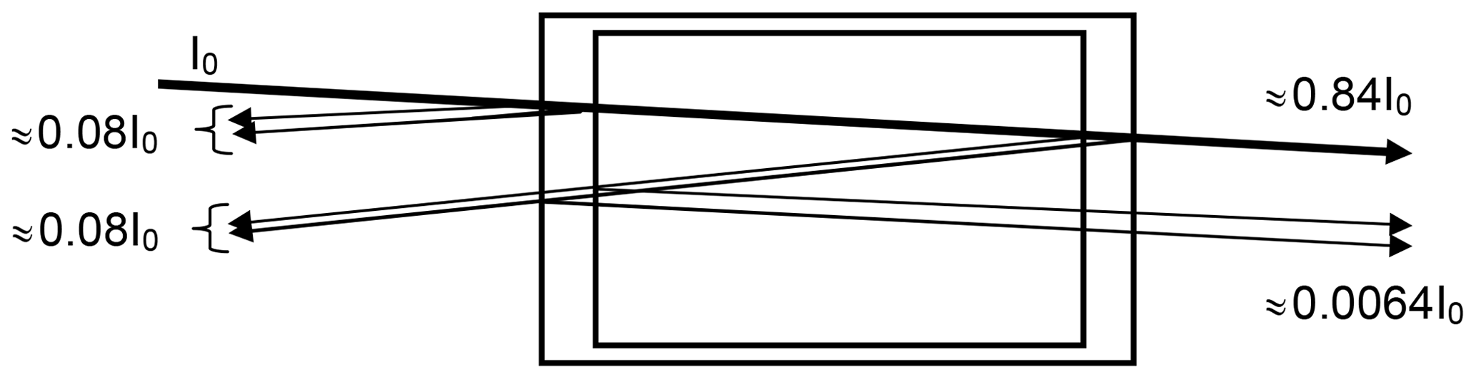
Figure 1Sketch of the optics of a gas absorption cell; parallel rays are assumed, and the (small) tilt of the incoming ray with respect to the cell axis is introduced to distinguish the rays. The described effect will also be there at strictly normal incidence. We assume an index of refraction of n=1.5 for the cell window material and accordingly 4 % reflection per surface (for near-normal incidence). Note that a fraction of about 0.69 % of the transmitted radiation passes the cell three times, thus adding ≈2 % to the total absorption (if the trace-gas absorption in the cell is small).
Thus a slight (few degrees) tilt of the cell will not lead to noticeable light path extension in the cell, but already a 1∘ tilt, leading to 0.015 % light path extension, would be sufficient to direct the multiple reflected light outside the field of view of the telescope. Thus, the additional 2 % cell absorption would disappear. On the other hand, larger tilts of the cell, for example of 10∘, would increase the cell absorption again by 1.5 % and should therefore be avoided. This could be accomplished by a rigid mount which fixes the (removable) cell at a defined angle with respect to the cell optical axis (normal of the windows), e.g. at 2∘.
As will be discussed below, the acceptance angle of the cell to ambient direct or scattered sunlight can play a significant role. Therefore, this small aperture angle allows for shielding the cell from sunlight, since solar radiation only needs to enter from a small solid angle (of the order of 10−3 sr), for instance, by mounting the cell inside a relatively long tube made of nontransparent material.
2.2 Path length in a cell as part of an optical system
In Sect. 2.1 we discussed the behaviour of an isolated cell; however the idea is to incorporate an absorption cell into an optical system, i.e. to just hold it in front of a MAX-DOAS instrument. In this case there can be interaction between the cell and the entrance optics of the instrument (for instance due to reflection of light at the surface of the telescope lens). As described by Lübcke et al. (2013) this can further enhance the trace-gas CD in the cell as seen by the instrument looking through it.
In the case of using gas cells in imaging instruments, for instance imaging spectrometers (e.g. Lohberger et al., 2004) or gas correlation instruments (e.g. Ward and Zwick, 1975), a larger aperture angle is required. This causes two potential problems. First, the aperture angle of the cell has to be much larger than in the case of a one-pixel (narrow field of view) instrument, for instance, typically a 30∘ total angle. Thus the acceptance angle for solar radiation becomes considerably larger (e.g. 0.22 sr instead of 10−3 sr), and consequently the photolysis frequencies for the gases inside the cell will be enhanced (see below). Second, the trace-gas CD of the cell becomes dependent on the observation angle ϑ (angle between the optical axis and the actual viewing direction within the field of view) as described above. For a total aperture angle of 30∘ this would amount to an enhancement of the SC(15∘) over of about 3.5 %.
Nitrogen dioxide (NO2) is a quite reactive gas (see rest of the section); therefore a series of chemical processes in an absorption cell can occur. Since they can alter the NO2 concentration – and thus the NO2 CD in the cell – considerably, they have to be watched. In the following subsections we discuss the relevant chemical processes, starting with important reactions and then proceeding to further reactions which are only relevant under certain conditions or if high accuracy is required.
We first discuss simplified chemistry, just encompassing the pertinent reactions, and then we proceed to a more comprehensive discussion of the chemistry in the following subsections.
3.1 The (initial) NO2-only chemistry – simple case
In a cell (initially) filled only with NO2 we can expect a series of reactions to occur, which are described in the following (bi-molecular rate constants are given in cm3 molec.−1 s−1, termolecular rate constants are given in cm6 molec.−2 s−1 for 25 ∘C and 1000 hPa, and details on temperature and pressure dependence as well as literature references can be found in Table 1). In fact, when buying NO2 from a manufacturer, some of the described reactions can already proceed in the initial gas, which therefore might already contain impurities (e.g. of NO, HONO, and HNO3).
Usually cells are exposed to sunlight or radiation needed for the measurement; thus NO2 in the cell can be photolysed:
The above value for J1 is reached in full sunshine around noontime (see e.g. Jones and Bayes, 1973 or Kraus and Hofzumahaus, 1998). Of course this figure (and in fact all photolysis frequencies in the cell; see Table 1) is highly variable, depending on solar zenith angle (i.e. latitude, season, and time of day), cloudiness, atmospheric turbidity, and the shading situation at the measurement site. In the case of active DOAS systems the photolysis frequencies will depend on the intensity of the light source and on the fraction of the cell cross-section area covered by the light beam. Nevertheless, it is frequently seen that calibration cells are used in full sunshine without any shielding; moreover, as is shown below (see Sect. 4), the effects on the NO2 chemistry are similar over a wide range of photolysis frequencies.
In the following, ground-state oxygen atoms O(3P) will be denoted by O. The threshold wavelength for Reaction (R1) is about 398 nm (e.g. Johnston and Graham, 1974; Burkholder et al., 2015); however, due to vibrational excitation of the ground-state molecule there is noticeable photolysis up to about 430 nm. If the cell is only illuminated with radiation of a wavelength longer than 430 nm, NO2 will not photolyse and J1 will be essentially zero.
Although it is only a small effect it is worth noting that the photolysis frequency inside a cell is not different from the value in the air surrounding the cell despite reflectance of the cell walls, as described by, for example, Bahe et al. (1979).
The oxygen atoms produced in Reaction (R1) can (1) recombine
However, this is a slow process, because the O-atom concentration will be very low (see Figs. 4 to 8). Alternatively, (2) O atoms may react with the wall where they predominantly recombine (see e.g. Cartry et al., 2000):
Also, (3) O atoms can react with NO2 to form NO:
Further, (4) oxygen atoms also may react with NO to form NO2:
The final possibility, (5) formation of NO3 – as well as further reactions, will be addressed in Sect. 3.4 below.
In addition there is the termolecular reaction of the O2 formed in Reactions (R4) or (R2) (or added to the cell filling) that oxidizes NO to NO2:
In an attempt to obtain a first-order quantitative understanding of the processes in the cell, we just consider a pure NO2 initial filling and Reactions (R1) (NO2 photolysis), (R4) (O+NO2), and (R6) (2NO+O2).
From the combination of Reactions (R1) and (R4) we derive the rates of NO and O2 formation under illumination,
which ultimately (i.e. in the stationary state) must equal the rate of NO destruction, D(NO) and NO2 formation, and P(NO2) due to Reaction (R6):
Since and the concentration of both species are zero initially, we have . Substituting this relationship,
and equating P(NO) with D(NO), we obtain
Further substituting ,
or
This cubic equation can be solved for the stationary-state NO concentration [NO]S as a function of the initial [NO2]0 as given in Appendix A.
Examples. (1) As an example, and to obtain a first idea of what might be happening in the cell, we assume about 1 atm (1000 hPa) of pure NO2 (initially); i.e. the initial NO2 concentrations in the cell will be cm−3 and the very simple chemical system just comprising Reactions (R1), (R4), and (R6). As we show below, the simplified reaction system – with the exception of the NO2 dimer (N2O4) formation (see Sect. 3.2) – is quite adequate. Also, such a cell would have a peak optical density (at around 440 nm) of about 14 at 1 cm length but much lower at other wavelengths.
In the dark (J1=0) nothing will happen, while in sunlight (): NO+O formation will take place followed by Reaction (R4) of NO2 with O. Thus the (initial) rate of NO formation P(NO) will be
This will lead to an initial decay time s. The stationary-state NO concentration can be calculated according to Eq. (7) and the solution given in Appendix A to be molec. cm−3, or about 10.7 % of the initial NO2 level. In other words, the NO2 concentration will be reduced to 89.3 % of its initial value [NO2]0. The corresponding NO rate of destruction will be
matching
from NO2 photolysis .
(2) We give a further example using about 1 hPa of pure NO2 (initially) corresponding to cm−3, and the same simple chemical system, just comprising Reactions (R1), (R4), and (R6), as above. Such a cell would have an initial differential optical density in the vicinity of 450 nm of about and would thus appear ideal to test the sensitivity of an NO2 spectrometer.
In sunlight we have cm−3 s−1. In this case, the resulting stationary-state NO level becomes , or about 100 % of the initial NO2. In other words after illumination the remaining NO2 concentration and thus the NO2 CD of the cell will only be a very small fraction of the expected value or cm−3, i.e. < 0.1 % of the initial [NO2]). After a short (of the order of 1 min) exposure to sunlight the NO2 in the cell will practically vanish.
On the other hand, in this simplified calculation, the NO reconversion, D(NO), to NO2 will be much slower than the initial photolysis:
Recovery from illumination. A further interesting question concerns the time for the chemical system to recover from a period of photolysis. Equation (4) gives the rate of NO destruction as a function of [NO]. In the case of example (1), above NO would decay with an initial rate of s−1 (ca. 11 % per second, suggesting a 9 s time constant for recovery). However, D(NO) varies with the third power of [NO]. When, for example, 90 % the NO is consumed (i.e. 1.4 % of [NO] is still left) the time constant would increase by a factor of 1000 to around 3 h.
In the case of example (2), the initial reconversion rate would only be s−1 (or ≈49 % per day), which would seem to imply a recovery time of somewhat more than 2 d. But again the dependence on the cube of the NO concentration means that the recovery time becomes much longer later on. For some model results, see Fig. 9.
3.2 The NO2↔N2O4 equilibrium
An additional problem in NO2 cells – in particular if high NO2 concentrations approaching 1000 hPa are used – is the formation of the dimer N2O4 (see also Roscoe et al., 1993):
There is a thermal decay of the dimer,
leading to an equilibrium with the equilibrium constant (298K; from Atkinson et al., 2004),
Note that the time to attain the equilibrium is shorter than µs (at 298 K and 1000 hPa). Thus, one can assume that there is always equilibrium between NO2 and N2O4. From this follows, for the [NO2]∕[N2O4] ratio,
What is usually most interesting is the fraction of NO2 of the total amount of NO2+N2O4 (i.e. pressure during filling) in the cell. The fraction is given by and thus
which can be transformed into
and solved for [NO2],
with the only positive solution:
or
The relationship between NO2 and [NO2]∕[NOZ] in the cell as a function of total is shown in Fig. 2.
For example, (1000 hPa or ca. 1 atm of total pressure, at 298 K), resulting in molec. cm−3 and . Thus, filling a cell from an NO2 reservoir (e.g. an NO2 tank) to 1 atm of total pressure will lead to only 34 % of this pressure being present as NO2 (see also Fig. 2).
At 100, 10, and 1 hPa (ca. 0.1, 0.01, and 0.001 atm) of NO2+N2O4, the corresponding figures for [NO2]1∕[NOZ] would be 0.717, 0.95, and 0.995, respectively. These figures are independent of an additional topping with air or oxygen to a full atmosphere of total pressure, as is described below. In other words, unless the NO2 partial pressure is below around 10 Pa, the actual NO2 partial pressure (and thus the concentration of NO2) will be below expected levels by two-digit percentages.
A further problem associated with the NO2–N2O4 equilibrium is the marked temperature dependence of the equilibrium constant. In the usual Arrhenius expression, it is given as
with cm−3 molec.−1 and B=6400 K (see Table 1). The (relative) temperature dependence of KEq is given by
and with the above values for A and B, we obtain, for the relative change in the equilibrium constant,
In other words the equilibrium constant is reduced by more than 7 % K−1 of heating. Fortunately the effect on NO2 is somewhat smaller, ranging from nearly zero change at very small NO2 levels to about a 3 % increase per degree of heating at 1000 hPa (see Appendix B).
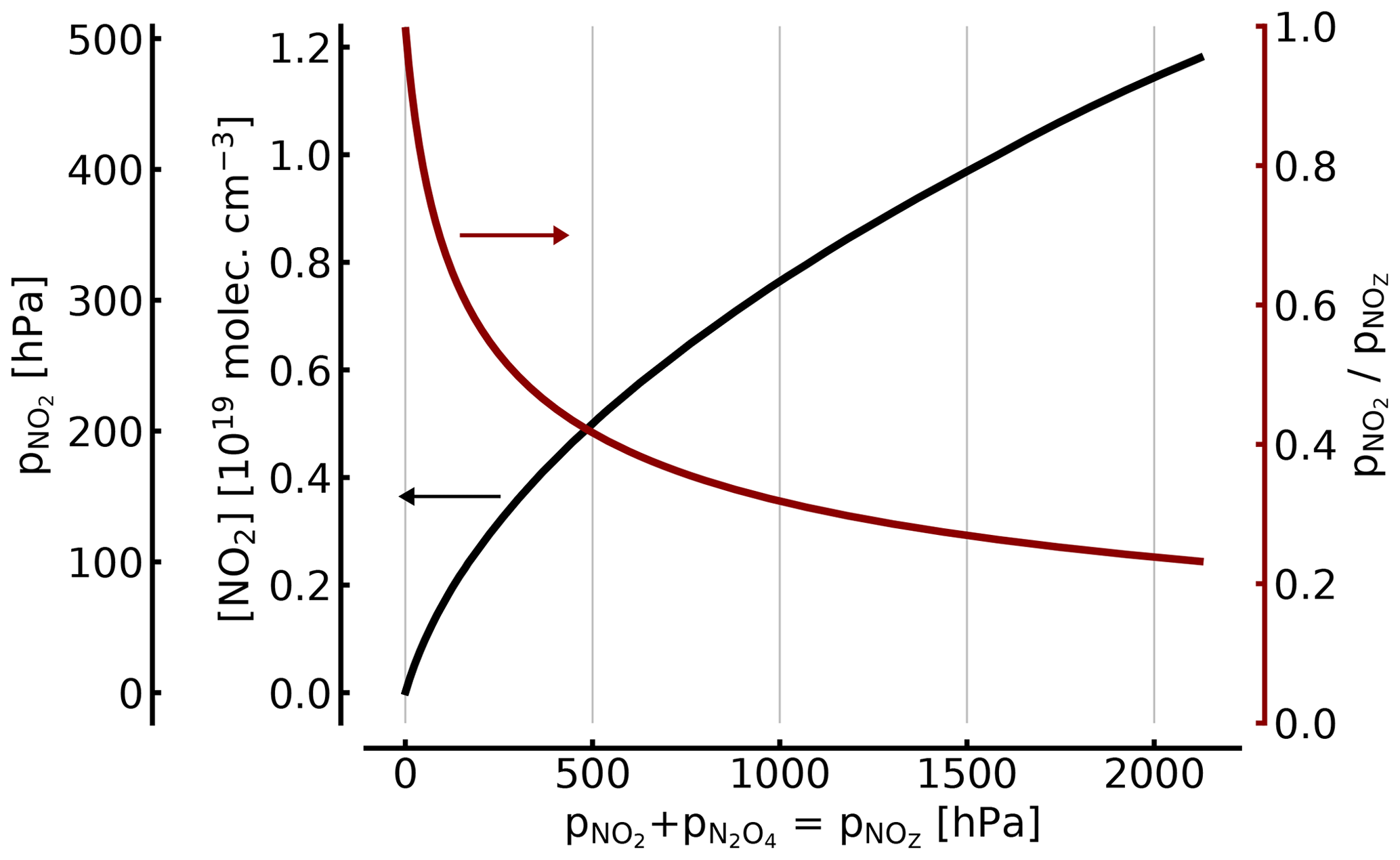
Figure 2NO2 concentration (black line in units of 1019 molec. cm−3 and hPa; left axes) and fraction of NO2 (red line; right axis) of the total as a function of [NOZ] (given in pressure units for 25 ∘C). At atmospheric pressure (1000 hPa) in the cell, only about 34 % of the total NOZ (or ≈344 hPa partial pressure) exists as NO2.
3.3 NO2+O2 chemistry
The addition of O2 (or air) to the NO2 filling can greatly help with stabilizing the NO2 concentration in a cell under certain conditions.
In the presence of molecular oxygen, following the photolysis of NO2, ozone is formed in the cell:
This in turn can react with NO to form NO2:
The reaction scheme encompassing the reaction pathways discussed above is sketched in Fig. 3.

Figure 3Scheme of the chemical reactions in an illuminated NO2 cell; (a) only basic reactions and (b) complete system excluding the formation of OH.
Here we can distinguish two regimes. The first regime assumes comparable concentrations of O2 and NO2, i.e. [O2]∕[NO2] around unity. In this case the termolecular oxidation of NO by O2 dominates. This is similar to the situation discussed in Sect. 3.1; however we can take the O2 concentration [O2] to be essentially constant. This reduces the third-order kinetics of Eq. (7) to pseudo-second-order or second-order kinetics, and we obtain
For example we may assume 0.5 atm (500 hPa) each of pure NO2 and O2 (initially); i.e. the initial concentrations of either species in the cell will be . In sunlight we have NO2 photolysis (Reaction R1) followed by O+NO2 (Reaction R4) plus oxidation of NO by O2;
From this stationary-state assumption we can calculate [NO]s:
Thus, the NO2 concentration would be reduced by only 5.4 % from its initial value once the cell is exposed to sunlight.
The second regime assumes a high [O2]∕[NO2] ratio (for instance larger than 104) so that the reaction of O atoms formed in NO2 photolysis is much more likely to react with O2 than with NO2. In this case for each molecule of NO2 photolysed nearly one molecule of O3 is formed, which will react with the NO molecule produced in the NO2 photolysis. The O3 concentration will rise until its reaction with NO balances the rate of NO2 photolysis:
Since [NO]≈[O3] we obtain
For instance at cm−3 and about 1 atm (1000 hPa) of O2, the stationary-state NO level would be cm−3, or about 1.8 % of the initial NO2 concentration. Note that a small fraction (about 10−4 in this example) of the O atoms produced in the NO2 photolysis would still react with NO2 and form NO without a corresponding O3 production (rate about 2×109 cm−3 s−1); thus the NO fraction in the cell would slowly grow until Reaction (R6) balances this process. At the above NO level the rate of NO2 formation would be around 109 cm−3 s−1; thus the NO level would slightly grow (by about 50 %) during several days of continuous illumination of the cell.
3.4 The (initial) NO2-only chemistry – some complications
In addition to the three reactions described above, O atoms can recombine with NO2 to form nitrate radicals, NO3:
The NO3 radicals formed in Reaction (R11) can be photolysed:
The threshold wavelength is much longer than in the case of NO2 (J1), and the photolysis is much faster. Alternatively, NO3 may react with NO (from Reaction R1) to re-form NO2,
or undergo self-reaction,
Finally, and typically most likely, NO3 will react with NO2 to form dinitrogen pentoxide, N2O5:
Dinitrogen pentoxide is thermally unstable and decays:
In the absence of water (dry system) N2O5 will just be another reservoir potentially sequestering some of the NO2. On the other hand, N2O5 is the anhydride of nitric acid and may react with water to form HNO3. While the reaction of N2O5 plus water vapour appears to be exceedingly slow in the gas phase, it may react with a layer at the cell surface; details are given in Sect. 3.5.
Analysing the above system of reactions, one notices that loss of O atoms other than by Reactions (R4) or (R11) are of minor importance. This is underlined by the results of the model calculations using the full chemical system (see Table 1) presented in Sect. 4.
Therefore, we can summarize that each photolysis Reaction (R1) is followed by a conversion of NO2 to NO (Reaction R4) or to NO3 (Reaction R11). However, NO3 is largely converted back to NO2 by Reactions (R12a), (R13), and (to a minor extent) (R14); thus, in effect each photolysis act of NO2 leads to the loss of approximately two NO2 molecules. Essentially NO2 would be converted to NO+O2. In bright sunshine with s−1, this would lead to an NO2 lifetime in the cell of s, or roughly 1 min. Even if the cell is kept in the shade or is only exposed to indoor illumination where J1 could be estimated to be 10 times (shade) to 100 times (indoor) smaller than in bright sunshine the conversion could be expected to proceed within around 10 min (shade) to 100 min (indoor) or even faster.
3.5 (trace) H2O chemistry
Since water is by far the most abundant (typical mixing ratios around 1 %) reactive trace gas in the ambient atmosphere (not counting nobel gases, CO2, H2, or N2O), it may be possible that if traces of water enter the cell when it is filled, then a series of additional reactions may play a role (see e.g. Bahe et al., 1979):
Followed by quenching of O(1D) to O(3P) or the formation of hydroxyl (OH) radicals,
In an NO2 cell, OH radicals are most likely to react with NO2 (or NO) to form nitric acid (or nitrous acid; see below):
Nitric acid is photolysed very slowly, and also its reaction with OH (to form NO3) is slow; thus it will constitute a final sink of NO2 (and water) in the cell. Alternatively, OH may react with NO to form nitrous acid:
which – in turn – is lost by photolysis,
In addition, N2O5, formed in Reaction (R15), can react with (liquid) water adsorbed at the wall of the cell, also forming HNO3:
Finally NO2 is also known to heterogeneously react with water:
Although this reaction appears to be second order in NO2, several studies (e.g. by Kleffmann et al., 1998) found a first-order dependence of HONO formation on the NO2 concentration probably because the NO2 reaction with NO2 adsorbed at the wall is rate limiting. Therefore, heterogeneous reactions of N2O4 with water are probably not important. HNO2 will photolyse relatively quickly to form OH + NO (with OH in most cases reacting according to Reaction R19); and HNO3 from the above two reactions will remain. Our model calculations actually show that all H2O is ultimately (typically after a few hours in full sunshine) converted to HNO3, sequestering equivalent amounts of NO2 and water; thus no HONO will remain after this time.
For example a cell having been filled with a very small amount of NO2 (e.g. 10 hPa or 2.4×10¹⁷ molec. cm−3) is topped with ambient (e.g. laboratory) air (which is of course not recommended; see Sect. 5.2) at 25 ∘C and 70 % relative humidity. Thus the approximate amount of water admitted is 70 % of the saturation vapour pressure of H2O at that temperature (70 % of 31.6 hPa = 22.1 hPa or 5.3×10¹⁷ molec cm−3). Some of this water will form a film at the inside of the cell and allow heterogeneous Reactions (R22) and (R23), converting NO2 into HNO3, although it is hard to judge how fast this process will proceed. In addition, upon illumination with UV-radiation Reactions (R9), (R17), (R18), and (R19) will provide (relatively slow) gas-phase conversion of NO2 to HNO3. Since the amount of H2O in this example exceeds the amount of NO2 it is likely that ultimately all NO2 is converted to HNO3, as can be seen in Figs. 4 to 8.
Table 1Summary of reaction rate constants.
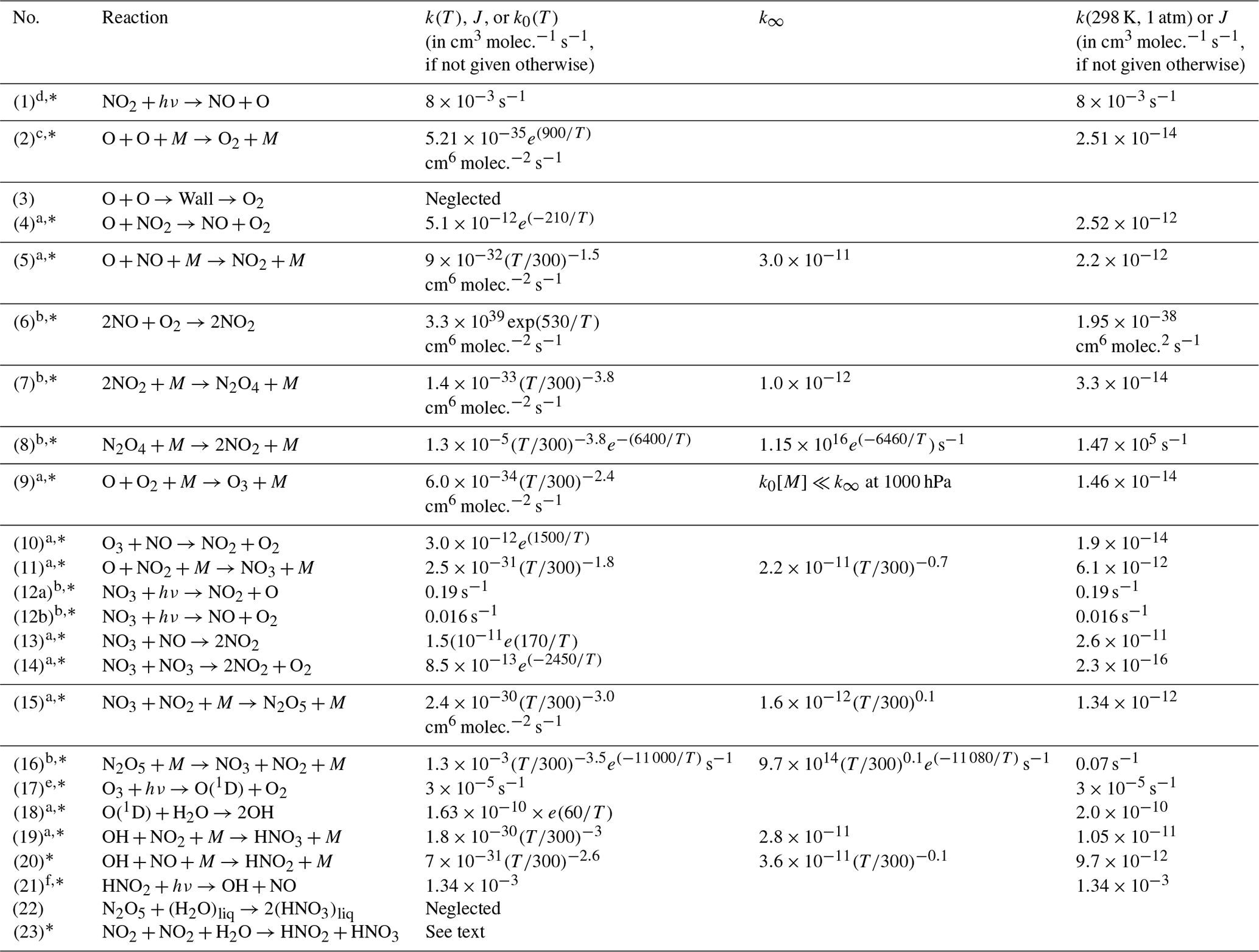
a Data from Burkholder et al. (2015) JPL Publication No. 15–10. b Data from Atkinson et al. (2004). c Data from Tsang and Hampson (1986). d Data from Trebs et al. (2009). e Data from Bahe and Schurath (1978). f Data from Alicke et al. (2002). The reactions marked with * are included in the kinetic model; see Sect. 4.
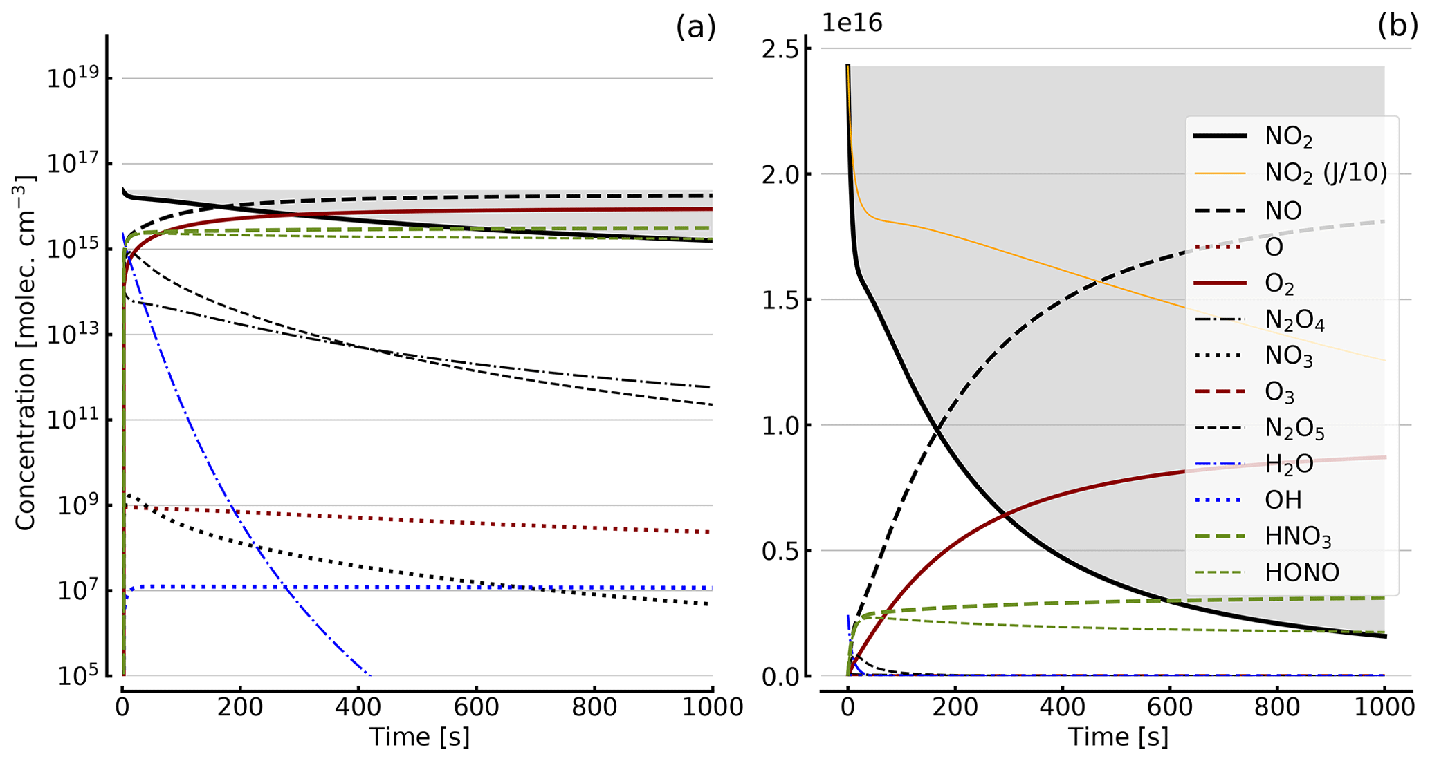
Figure 4Results of calculations with the full model (reactions marked with * in Table 1). Shown are the temporal evolutions of [NO2], [NO2] with J values scaled to 1∕10, [NO], [O], [O2], [O3], [N2O4], [NO3], [N2O5], [H2O], [OH], [HNO3], and [HONO] in an illuminated NO2 cell. Initial [NO2]0=1 hPa (2.4×10¹⁶ molec. cm−3). Zero initial O2 concentration was assumed; (a) logarithmic scale and (b) linear scale.
We performed a series of gas-kinetic-simulation calculations in order to illustrate the behaviour of the reaction system described above under various conditions of initial NO2 and amounts of added O2. In a one-box model, the system of coupled ordinary differential equations resulting from the above reactions was solved numerically. This allows following the temporal evolution of the concentration of the individual gases in the cell under given conditions. Our full model includes Reactions (R1) to (R23), except (R3) and (R22) of Table 1 (marked with an asterisk in column 1). The heterogeneous Reaction (R23) was included in the simulation, with the parameterization proposed by Kleffmann et al. (1998) , with uptake coefficient , the molecular velocity of NO2 v, and the surface-to-volume ratio S∕V). We assumed a typical cell (cylindrical, radius of 1 cm, and length of 5 cm, m−1) as well as estimates of the amount of H2O in this cell from assuming a monolayer of water at the inner surface of the cuvette. Of course – given the uncertainties in heterogeneous reactions – this approach can only provide a rough estimate of the HONO concentration in the cell.
Also some runs with a subset of the reactions were performed as described in Appendix B in order to check on the simplified analytical calculations in the previous section. Table 2 shows a comparison of the NO2 reduction after 1000 s given by the analytical calculations and the simplified model.
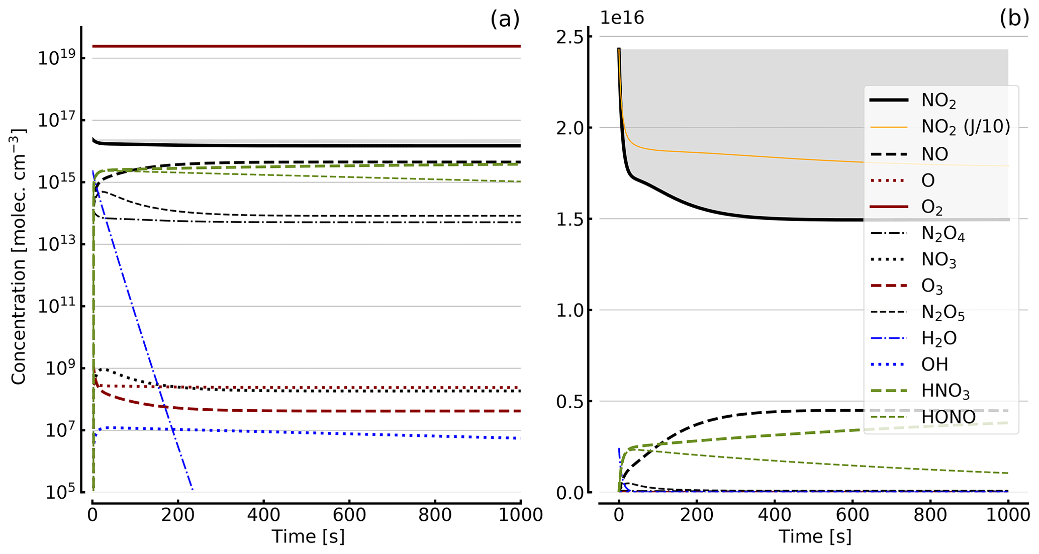
Figure 5Results of calculations with the full model (reactions marked with * in Table 1). Same as Fig. 4, but with initial O2 assumed; (a) logarithmic scale and (b) linear scale.
Table 2Comparison of the analytical calculations and the simplified model encompassing Reactions (R1), (R4), and (R6).
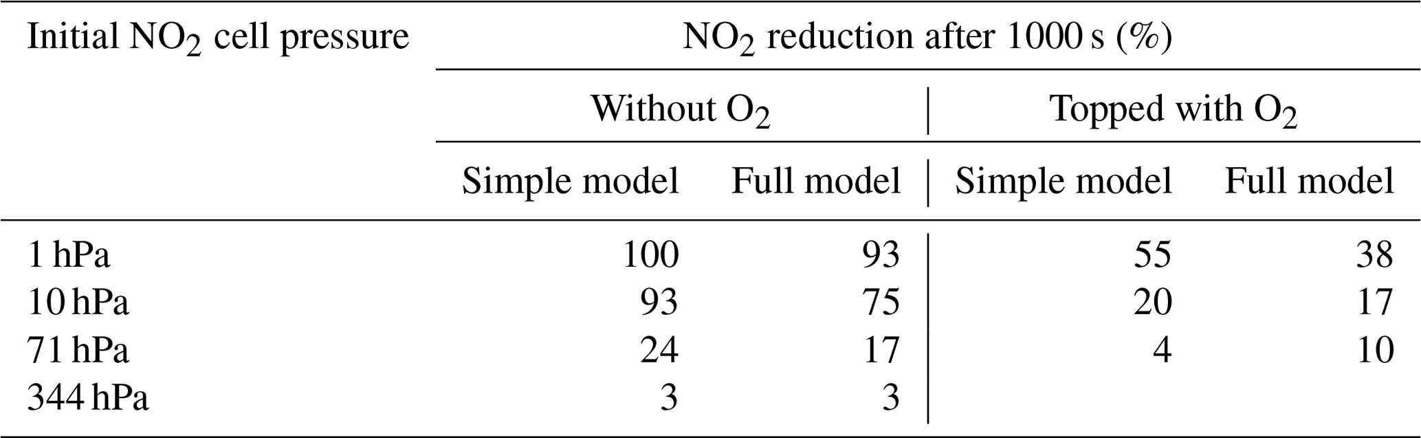
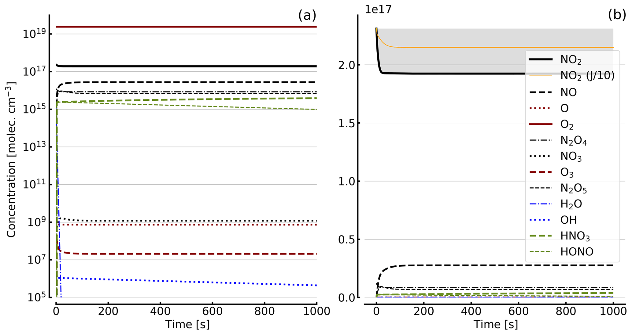
Figure 6Results of calculations with the full model (reactions marked with * in Table 1). Same as Fig. 5, but initial [NO2]0=10 hPa (2.4×10¹⁷ molec. cm−3) with initial O2 assumed; (a) logarithmic scale and (b) linear scale.
Further calculations encompass the full range of Reactions (R1) to (R23), except (R3) and (R22) as given in Table 1 (marked with an asterisk), where an analytical solution is not practical or is probably even impossible. Figures 4 to 8 show the results of these model runs for NO2, NO, O atoms, O2, N2O4, NO3, O3, N2O5, H2O, OH, HNO3, and HONO in an illuminated NO2 cell for initial, N2O4-equilibrated [NO2]0 of 1, 10, 71, and 344 hPa (2.4×10¹⁶, 2.4×10¹⁷, 1.7×10¹⁸, and 0.84×10¹⁹ molec. cm−3). In Fig. 4 no initial O2 was assumed, and the remaining figures (Figs. 5 to 8) show time series with initial O2. The left and right panels have logarithmic and linear concentration scales, respectively. Comparison of the result with the data in Figs. 5 to 8 shows that there are no fundamental differences in the NO2 time series between the simple model and the full model (see also Table 2).
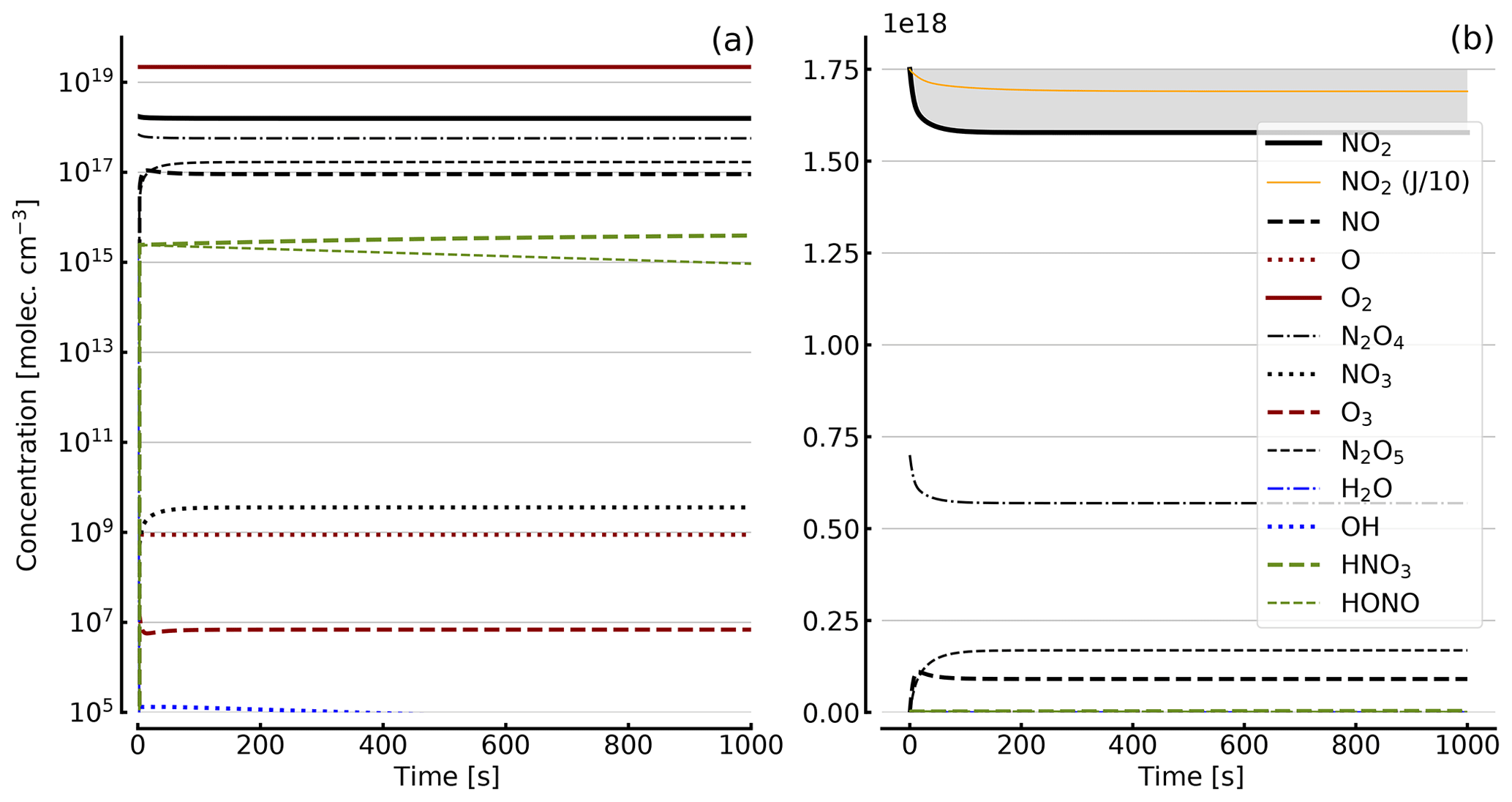
Figure 7Results of calculations with the full model (reactions marked with * in Table 1). Same as Fig. 5, but initial [NO2]0=71 hPa (1.7×10¹⁸ molec. cm−3) with initial O2 assumed; (a) logarithmic scale and (b) linear scale.
In order to study the effect of different photolysis frequencies, we also performed model runs with all J values scaled to 1∕10 of the figures given in Table 1. The resulting temporal evolutions of NO2 are also included in Figs. 4 to 8 (note that the time series of all other species are for the J values as given in Table 1). As can be seen from these figures there is still a rather large loss of NO2, even with J being only 1∕10 of its value in full sunshine. This is due to the fact that the NO2 loss scales only with the second or third root of the photolysis frequency (see analytical solutions in Sect. 3 and Appendix A).
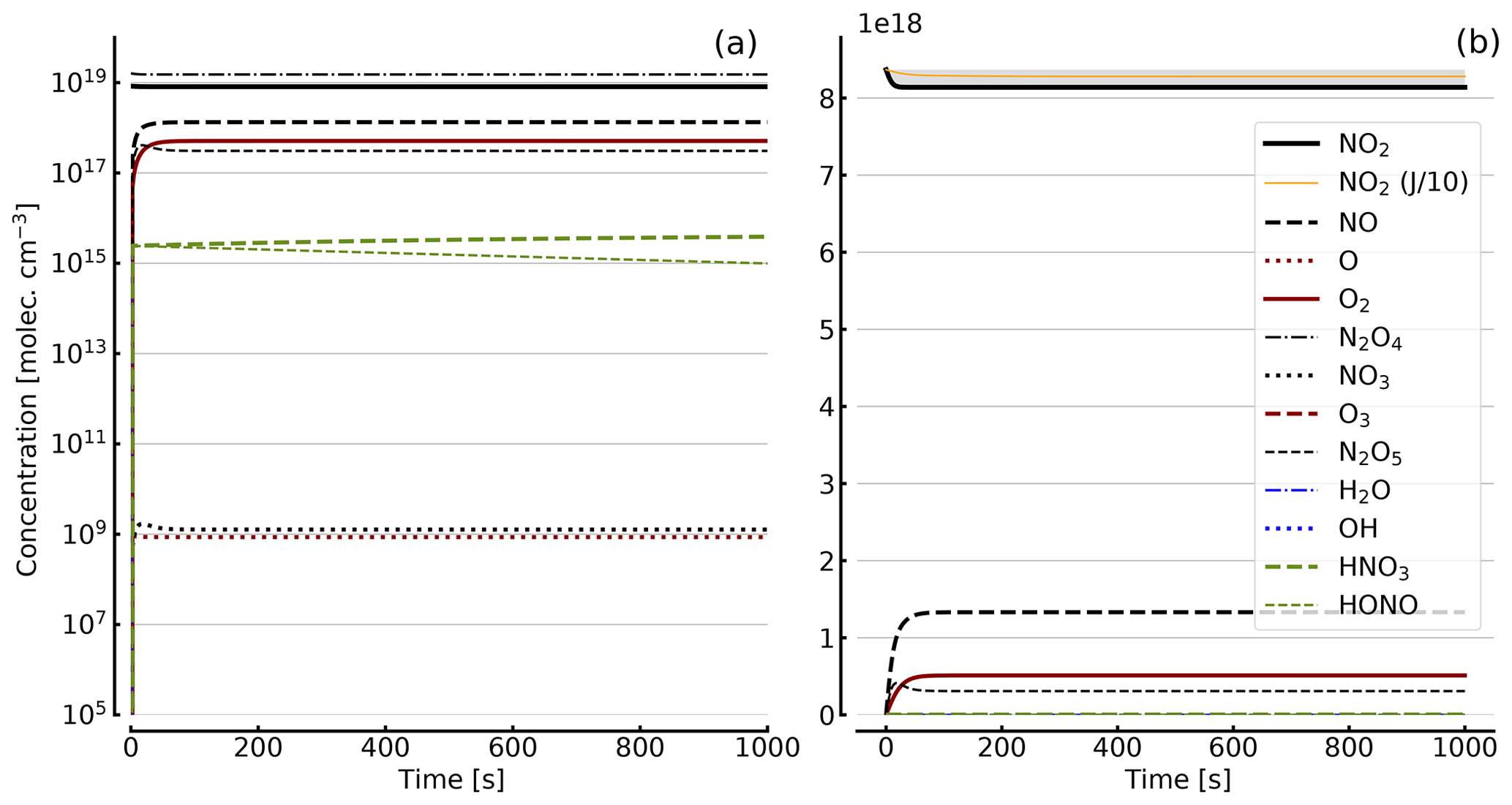
Figure 8Results of calculations with the full model (reactions marked with * in Table 1). Same as Fig. 5, but initial [NO2]0=344 hPa (0.84×10¹⁹ molec. cm−3) with initial O2 assumed; (a) logarithmic scale and (b) linear scale.
As discussed in Sect. 3.1 the recovery of NO2 in the dark after initial illumination (e.g. due to a use of the cell in a measurement) is an important question. Figure 9 shows model calculations of the temporal evolution of NO2, NO, and O2 according to the full model (Reactions R1 to R23, except Reactions R3 and R22 – see Table 1; at 298 K). The NO2 cell is initially illuminated for 1500 s and then left in the dark afterwards for initial, N2O4-equilibrated [NO2]0 of 1, 10, 71, and 344 hPa (2.4×10¹⁶, 2.4×10¹⁷, 1.7×10¹⁸, and 0.84×10¹⁹ molec. cm−3, respectively). At the two highest [NO2]0 levels the initial NO2 was chosen such that total pressures of 100 and 1000 hPa were reached. It can be seen that the NO2 recovery at low NO2 levels can take days to hours. Adding O2 to the cell again has a strong impact on the [NO2] evolution (see thin blue lines in Fig. 7), reducing the recovery time to a fraction of the NO2-only case. For larger initial NO2 concentrations (e.g. 71 hPa) and added O2, a hysteresis between initial [NO2] and equilibrium [NO2] in the dark can be observed; i.e. the NO2 level does not return to its initial value after illumination. This is due to the formation of N2O5 in the illuminated period.
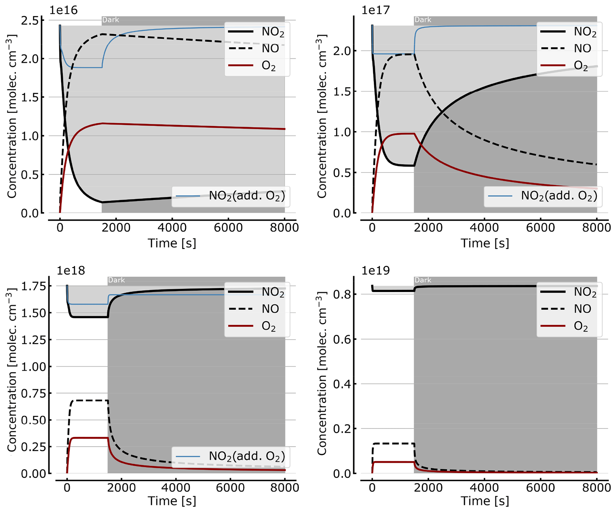
Figure 9Recovery of NO2 in the dark after initial illumination. Model calculations of the temporal evolution of [NO2] (thick solid black line), [NO] (dashed black line), and [O2] (solid brown line) calculated with the full model (reactions marked with * in Table 1). The NO2 cell is initially illuminated for 1500 s and then left in the dark afterwards. Initial [NO2]0 of 1, 10, 71, and 344 hPa (2.4×10¹⁶, 2.4×10¹⁷, 1.7×10¹⁸, and 0.84×10¹⁹ molec. cm−3). The blue thin line in the plots for 1, 10, and 71 hPa show [NO2] for O2-topped-up cell.
We conclude that the use of NO2 cells requires careful consideration, in particular when quantitative measurements of the NO2 CD in the cell are desired. If unfortunate parameters are chosen (e.g. rather low NO2 pressures or no O2 or air added), practically no NO2 might be found in the cell at all. Also, one cannot conclude that particularly high or low NO2 concentrations in the cell are the superior choice. At high NO2 concentrations (approaching atmospheric pressure) a large fraction of the NO2 is converted to the dimer N2O4, which not only reduces the NO2 CD way below expected values but also introduces a large temperature dependence (up to 3 % per degree) of the NO2 CD in the cell (also, there might be some additional uncertainty due to uncertainty of the equilibrium constant, as pointed out by Roscoe and Hind, 1993). On the other hand, at low NO2 levels (e.g. 1 hPa) photolysis may convert much (if not virtually all) of the NO2 to NO. Although NO2 eventually recovers, this process may take long (days) to complete. Thus, the actual NO2 CD of the cell may become dependent on the illumination and recovery history of the cell and may be rather unpredictable for a particular cell.
Unfortunately, the two described effects are not even the full story; therefore the potential problems are listed below. Fortunately, there are ways to minimize the problems, like oxygen addition to the cell and choosing the right NO2 concentration, which may help in reducing the uncertainty of the NO2 CD of a given cell to the single-digit percentage range.
5.1 Summary of problems
As discussed above, the NO2 concentration in a cell – and thus the NO2 CD of the cell – can deviate from expectations due to a number of reasons:
-
Optical effects, namely multiple reflection in the cell and tilt of the cell with respect to the optical axis, can enhance the light path and thus the apparent NO2 CD.
-
Photolysis of NO2 can reduce the NO2 CD in the cell.
-
Sequestration of NO2 as N2O4 due to the thermodynamic equilibrium between the two species can reduce NO2 in the cell and cause temperature dependence of the NO2 CD.
-
Formation or re-formation of NO2 from NO in the cell leads to slow recovery of NO2.
-
Irreversible conversion or conversion of NO2 to HNO3 can lead to long-term loss of NO2.
-
Wall loss of NOX species like N2O4 or N2O5 can lead to long-term loss of NO2
5.2 Some ideas to remedy the situation
One approach for minimizing loss of NO2 in the cell is certainly to reduce the photolysis of NO2 (Reaction R1); this can be achieved by a series of measures.
-
Only expose the cell to measurement radiation by, for example, putting it in a nontransparent tube.
-
Minimize exposure time by, for example, putting the cell in a light-tight box when not in use.
-
Use a filter in front of the cell which only admits radiation at wavelengths > 450 nm; this, however, may interfere with the measurements.
Also, it may be good to avoid ozone photolysis in the cell to minimize OH formation by using a UV-nontransparent cell material, e.g. glass instead of quartz. In addition, it is a good idea to keep the gas in the cell as dry as possible to avoid formation of HNO3 or HNO2 and to further minimize OH formation. Furthermore, it may be a good idea to illuminate a freshly filled cell initially (for a few hours) to allow all remaining water to be converted to HNO3, thus (1) minimizing later changes in the NO2 concentration due to HNO3 formation and (2) avoiding HONO formation.
A further important measure is to add O2 to the cell in order to enhance reconversion of any NO formed to NO2.
The problems associated with excessive N2O4 formation in the cell (reduction of the NO2 CD, temperature dependence of the NO2 CD, and HNO3 formation) can be reduced by using lower NO2 concentrations in the cell. The length of the cell may need to be extended to still achieve a desired NO2 CD. In principle the cell may also be heated to lower the amount of steady-state N2O4.
Problems with the optics of the cell are also difficult to avoid; fortunately they usually lead to changes in the NO2 CD of < 10 %. In principle wedged cell windows or anti-reflective coatings could be used on the cell windows to minimize the problems described in Sect. 2. Another approach would be to tilt the entire cell with respect to the optical axis; thus reflected radiation would not reach the entrance optics of the spectrometer.
The model data can be obtained from the authors upon request.
The above Eq. (7) is a cubic equation, which we recognize as Cardano's formula after substituting z=[NO]:
for which the solution is well known as (Bronstein et al., 2013)
with
and
Equation (7) for z=[NO] thus becomes
It is transformed with molec.2 cm−6 to
Sample solutions include the following.
-
1000 hPa of initial NO2, i.e. , with p=a and , and
we obtain the only positive and real solution:
This means that [NO]∕[NO2]0 is about % of the initial NO2.
-
At 100 hPa of initial NO2 ([NO2]0= 2.4×10¹⁸), we obtain % of the initial NO2.
-
At 10 hPa of initial NO2 ([NO2]0= 2.4×10¹⁷), we obtain % of the initial NO2.
-
At 1 hPa of initial NO2, ([NO2]0= 2.4×10¹⁶), we obtain % of the initial NO2.
Reaction kinetic box-model calculations show the temporal evolution of [NO2], [NO], and [O2], according to the simple reaction system (Reactions R1, R4, and R6) in an illuminated NO2 cell. In addition we initially neglect the NO2 dimer formation. These calculations merely serve to demonstrate that the analytical solution as derived in Sect. 3.1 matches the model calculations.
Figure B1 shows some results of this oversimplified model, assuming (as above) initial NO2 levels [NO2]0 of 1, 10, 100, and 1000 hPa (2.4×10¹⁶, 2.4×10¹⁷, 2.4×10¹⁸, and 2.4×10¹⁹ molec. cm−3, respectively). As expected the initial NO2 concentration drops within the first few seconds (at high initial NO2) to minutes (at low NO2) until the back reaction kicks in and leads to stationary-state levels of all species after this initial period. At 1 hPa of initial NO2 its concentration drops to very small levels (< 0.1 %), as shown in Sect. 3.1, while at 1000 hPa we still see about a 10.7 % loss of initial NO2. These figures are exactly the same as those found from the steady-state calculations (see Appendix A).
Figure B2 shows some results of the simplified model (Reactions R1, R4, and R6), but including the NO2–N2O4 equilibrium (Reactions R7 and R8) for initial NO2 levels, [NO2]0 of 1, 10, 71, 344 hPa (2.4×10¹⁶, 2.4×10¹⁷, 1.7×10¹⁸, 0.84×10¹⁹ molec. cm−3, due to filling the cell with NO2 levels of 1, 10, 100, and 1000 hPa, respectively, which then immediately undergo N2O4 equilibration). For the lower initial NO2 levels (1 and 10 hPa), there is little difference to Fig. B1. The initial NO2 concentration drops within the first few seconds to minutes to small fractions of the initial [NO2]0. As discussed above (Sect. 3.3), the situation can be improved by adding initial O2 (topped up to 1000 hPa). The thin blue line in the plots for [NO2]0 of 1, 10, and 71 hPa indicates the results for the corresponding NO2 profiles. In particular at higher initial NO2 levels (e.g. 71 hPa) the ultimate NO2 levels are considerably enhanced by O2 addition. However at higher initial NO2 levels (see plots for 71 and 344 hPa initial NO2) there is a large reduction in NO2 due to the NO2-dimer formation, inducing stronger temperature dependence.
In order to get a feeling for the influence of temperature changes in the model run for [NO2]0=344 hPa the temperature was raised by 5 K (298 to 303 K) after 100 s; the corresponding plot (bottom right in Fig. B2) shows an increase in NO2 (thin blue line) of about 16 % due to this temperature rise.
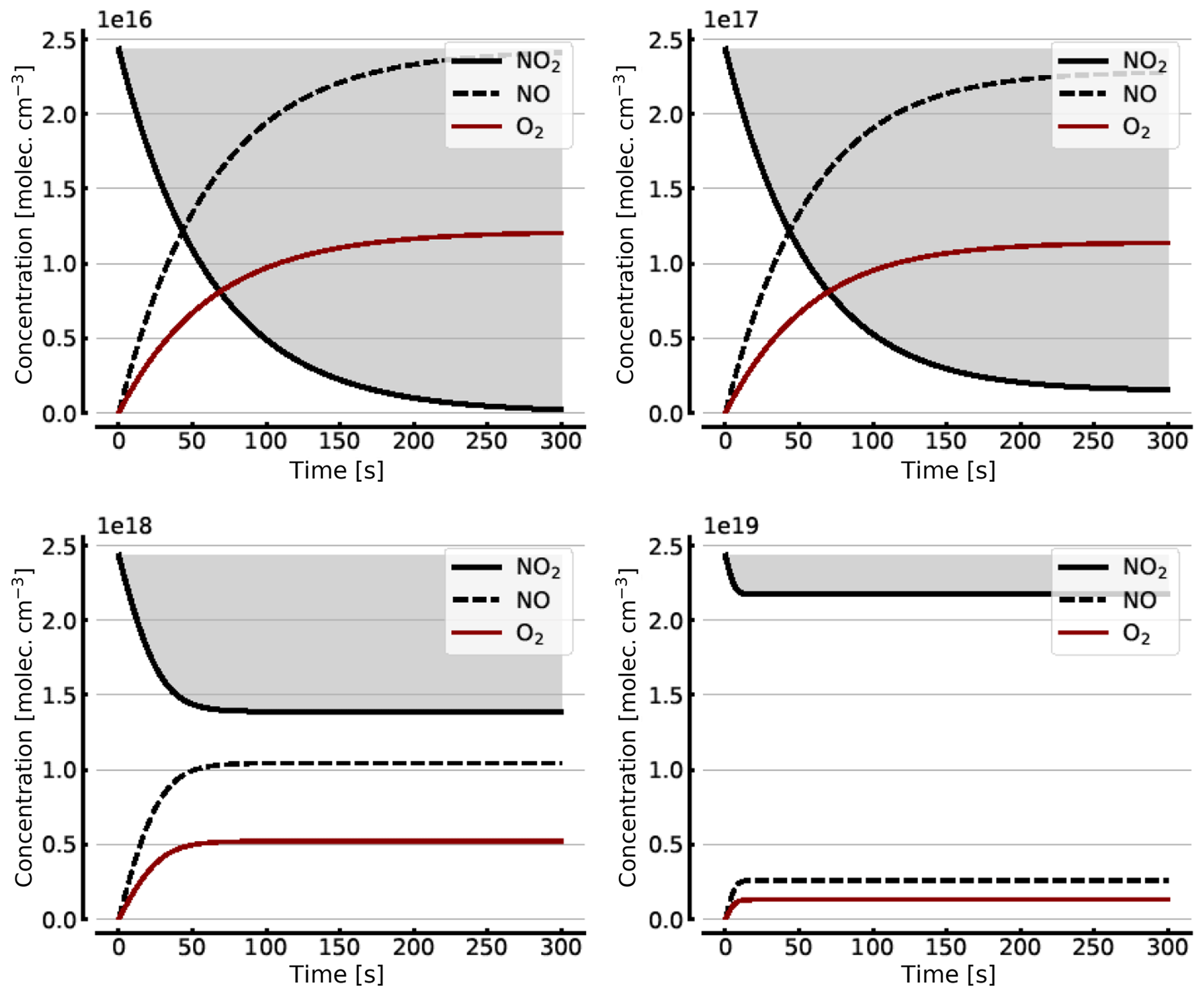
Figure B1Model calculations of the temporal evolution of [NO2] (thick solid black line), [NO] (dashed black line), and [O2] (solid brown line) according to the simple reaction system (Reactions R1, R4, and R6 only, at 298 K) in an illuminated NO2 cell. Here the NO2–N2O4 chemical equilibrium is neglected, which makes in particular the plots for initial [NO2]0=1000 hPa unrealistic. All time series are for calculation with no added initial O2. Initial [NO2]0 of 1, 10, 100, and 1000 hPa (2.4×10¹⁶, 2.4×10¹⁷, 2.4×10¹⁸, and 2.4×10¹⁹ molec. cm−3, respectively).
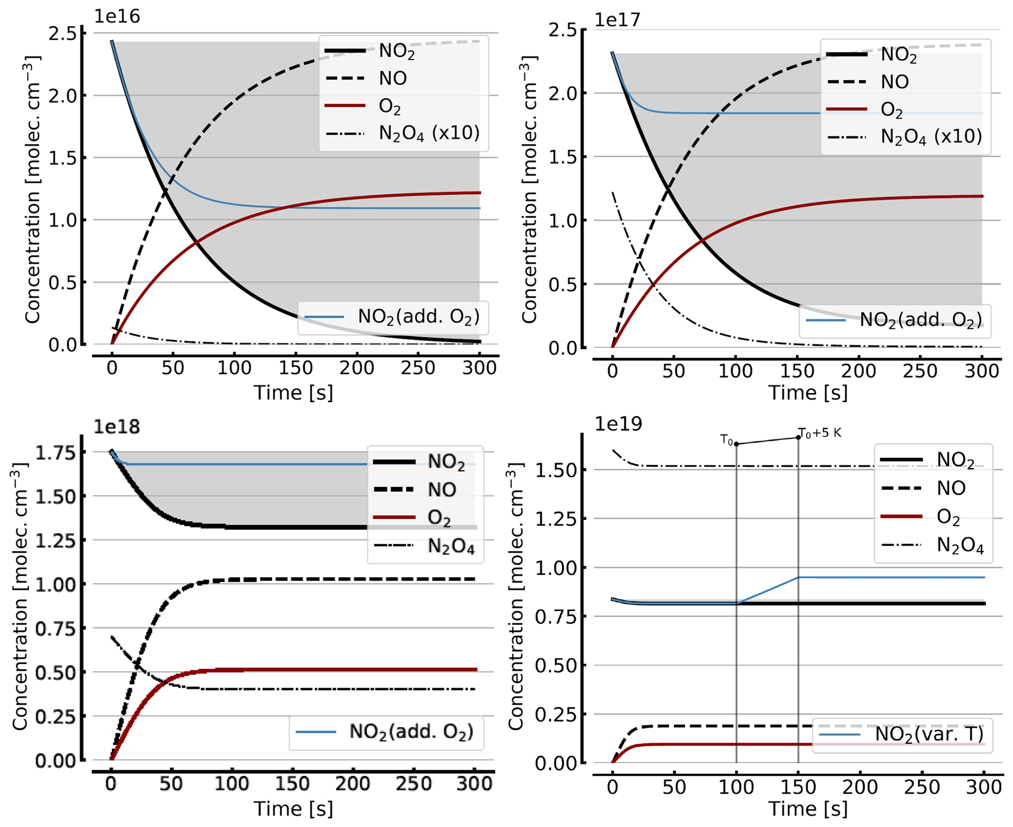
Figure B2Same model calculations as shown in Fig. B1, but including N2O4. Initial [NO2]0 of 1, 10, 71, and 344 hPa (2.4×10¹⁶, 2.4×10¹⁷, 1.7×10¹⁸, and 0.8×10¹⁹ molec. cm−3, respectively; see text). Temporal evolution of [NO2] (thick solid black line), [NO] (dashed black line), [O2] (solid brown line), and [N2O4] (thin dashed–dotted line; ×10 in the upper two panels) according to the simple reaction system (Reactions R1, R4, R6, R7, and R8 only, at 298 K) in an illuminated NO2 cell. All time series with the exception of the thin blue line (in the plots for [NO2]0=1, 10, and 71 hPa) are for calculation with no added initial O2. The thin blue line (in the plots for [NO2]0 of 1, 10, and 71 hPa) indicates the evolution of NO2 for a calculation with initial O2 topped up to 1000 hPa. The plot for [NO2]0=344 hPa additionally shows the increase in NO2 (thin blue line) at a temperature rise of 5 K (298 to 303 K).
Both authors developed the concept of the paper and discussed its contents. UP wrote most of the text, and JK performed the model calculations.
The authors declare that they have no conflict of interest.
Partial support by the DFG project 193/18-3 is gratefully acknowledged. We also thank two anonymous reviewers for valuable and constructive comments.
The article processing charges for this open-access publication were covered by the Max Planck Society.
This paper was edited by Hendrik Fuchs and reviewed by two anonymous referees.
Alicke, B., Platt, U., and Stutz, J.: Impact of nitrous acid photolysis on the total hydroxyl radical budget during the Limitation of Oxidant Production/Pianura Padana Produzione di Ozono study in Milan, J. Geophys. Res., 107, 8196, https://doi.org/10.1029/2000JD000075, 2002.
Atkinson, R., Baulch, D. L., Cox, R. A., Crowley, J. N., Hampson, R. F., Hynes, R. G., Jenkin, M. E., Rossi, M. J., and Troe, J.: Evaluated kinetic and photochemical data for atmospheric chemistry: Volume I – gas phase reactions of Ox, HOx, NOx and SOx species, Atmos. Chem. Phys., 4, 1461–1738, https://doi.org/10.5194/acp-4-1461-2004, 2004.
Bahe, F. and Schurath, U.: Measurement of O(1D) Formation by Ozone Photolysis in the Troposphere, Pure Appl. Geophys., 116, 537–544, 1978.
Bahe, F. C., Marx, W. N., Schurath, U., and Röth, E. P.: Determination of the absolute photolysis rate of ozone by sunlight at ground level, Atmos. Environ., 13, 1515–1522, 1979.
Bronstein, I. N., Mühlig, H., Musiol, G., and Semendjajew, K. A.: Taschenbuch der Mathematik (Bronstein), Verlag Europa-Lehrmittel, Nourney, Vollmer GmbH & Co. KG, Haan-Gruiten, Germany, 2013.
Burkholder, J. B., Sander, S. P., Abbatt, J., Barker, J. R., Huie, R. E., Kolb, C. E., Kurylo, M. J., Orkin, V. L., Wilmouth, D. M., and Wine, P. H.: Chemical Kinetics and Photochemical Data for Use in Atmospheric Studies, Evaluation No. 18, JPL Publication 15-10, Jet Propulsion Laboratory, Pasadena, available at: http://jpldataeval.jpl.nasa.gov (last access: 24 October 2019), 2015.
Cartry, G., Magne, L., and Cernogora, G.: Atomic oxygen recombination on fused silica: modelling and comparison to low-temperature experiments (300 K), J. Phys. D Appl. Phys., 33, 1303–1314, 2000.
Hönninger, G. and Platt, U.: The Role of BrO and its Vertical Distribution during Surface Ozone Depletion at Alert, Atmos. Environ., 36, 2481–2489, 2002.
Johnston, H. S. and Graham, R.: Photochemistry of NOx and HNOx Compounds, Can. J. Chem., 52, 1415–1423, 1974.
Jones, I. T. N. and Bayes, K. D.: Photolysis of nitrogen dioxide, J. Chem. Phys., 59, 4836, https://doi.org/10.1063/1.1680696, 1973.
Kebabian, P. L., Annen, K. D., Berkoff, T. A., and Freedman, A.: Nitrogen dioxide sensing using a novel gas correlation detector, Meas. Sci. Technol., 11, 499–503, 2000.
Kleffmann, J., Becker, K. H., and Wiesen, P.: Heterogeneous NO2 conversion processes on acid surfaces: possible atmospheric implications, Atmos. Environ., 32, 2721–2729, 1998.
Kraus, A. and Hofzumahaus, A.: Field Measurements of Atmospheric Photolysis Frequencies for O3, NO2, HCHO, CH3CHO, H2O2, and HONO by UV Spectroradiometry, J. Atmos. Chem., 31, 161–180, 1998.
Lohberger, F., Hönninger, G., and Platt, U.: Ground Based Imaging Differential Optical Absorption Spectroscopy of Atmospheric Gases, Appl. Opt., 43, 4711–4717, 2004.
Lübcke, P., Bobrowski, N., Illing, S., Kern, C., Alvarez Nieves, J. M., Vogel, L., Zielcke, J., Delgado Granados, H., and Platt, U.: On the absolute calibration of SO2 cameras, Atmos. Meas. Tech., 6, 677–696, https://doi.org/10.5194/amt-6-677-2013, 2013.
Platt, U. and Stutz, J.: Differential Optical Absorption spectroscopy, Principles and Applications, XV, Springer, Heidelberg, 597 pp., 2008.
Roscoe, H. K. and Hind, A. K.: The equilibrium constant of NO2 with N2O4 and the temperature dependence of the visible spectrum of NO2: A critical review and the implications for measurements of NO2 in the polar stratosphere, J. Atmos. Chem., 16, 257–276, https://doi.org/10.1007/BF00696899, 1993.
Sandsten, J., Edner, H., and Svanberg, S.: Gas imaging by infrared gas-correlation spectrometry, Optics Lett., 21, 1945–1947, 1996.
Sandsten, J., Edner, H., and Svanberg, S.: Gas Visualization of industrial hydrocarbon emissions, Opt. Exp., 12, 1443–1451, 2004.
Tsang, W. and Hampson, R. F.: Chemical Kinetic Data Base for Combustion Chemistry, Part I, Methane and Related Compounds, J. Phys. Chem. Ref. Data, 15, 1087–1279, 1986.
Trebs, I., Bohn, B., Ammann, C., Rummel, U., Blumthaler, M., Königstedt, R., Meixner, F. X., Fan, S., and Andreae, M. O.: Relationship between the NO2 photolysis frequency and the solar global irradiance, Atmos. Meas. Tech., 2, 725–739, https://doi.org/10.5194/amt-2-725-2009, 2009.
Ward, T. V. and Zwick, H. H.: Gas cell correlation spectrometer: GASPEC, Appl. Opt., 14, 2896–2904, 1975.
- Abstract
- Introduction
- Optics of cells
- Chemistry in NO2-absorption cells
- Gas kinetic simulations
- Summary and conclusions
- Data availability
- Appendix A: Solution of the cubic equation for the stationary-state NO concentration
- Appendix B: The simplified model
- Author contributions
- Competing interests
- Acknowledgements
- Financial support
- Review statement
- References