Improving the mean and uncertainty of ultraviolet multi-filter rotating shadowband radiometer in situ calibration factors: utilizing Gaussian process regression with a new method to estimate dynamic input uncertainty

To recover the actual responsivity for the Ultraviolet Multi-Filter Rotating Shadowband Radiometer (UV-MFRSR), the complex (e.g., unstable, noisy, and with gaps) time series of its in situ calibration factors (V₀) need to be smoothed. Many smoothing techniques require accurate input uncertainty of the time series. A new method is proposed to estimate the dynamic input uncertainty by examining overall variation and subgroup means within a moving time window. Using this calculated dynamic input uncertainty within Gaussian process (GP) regression provides the mean and uncertainty functions of the time series. This proposed GP solution was first applied to a synthetic signal and showed significantly smaller RMSEs than a Gaussian process regression performed with constant values of input uncertainty and the mean function. GP was then applied to three UV-MFRSR V₀ time series at three ground sites. The method appropriately accounted for variation in slopes, noises, and gaps at all sites. The validation results at the three test sites (i.e., HI02 at Mauna Loa, Hawaii; IL02 at Bondville, Illinois; and OK02 at Billings, Oklahoma) demonstrated that the agreement among aerosol optical depths (AODs) at the 368 nm channel calculated using V₀ determined by the GP mean function and the equivalent AERONET AODs were consistently better than those calculated using V₀ from standard techniques (e.g., moving average). For example, the average AOD biases of the GP method (0.0036 and 0.0032) are much lower than those of the moving average method (0.0119 and 0.0119) at IL02 and OK02, respectively. The GP method's absolute differences between UV-MFRSR and AERONET AOD values are approximately 4.5 %, 21.6 %, and 16.0 % lower than those of the moving average method at HI02, IL02, and OK02, respectively. The improved accuracy of in situ UVMRP V₀ values suggests the GP solution is a robust technique for accurate analysis of complex time series and may be applicable to other fields.

1 Introduction

While many instruments generate relatively stable data time series over short time windows, dynamic uncertainty levels, variable sampling densities, and/or different lengths of gaps with missing data can complicate the analysis of long-term datasets. For example, the 5-year time series of a solar variability indicator (Mg II core to wing index) shows consistency on the order of days but increasing noise level and gaps are observed at the month scale (Cebula et al., 1992). The time series of the geopotential scale factor, a function of the geoidal potential, is also relatively stable on shorter timescales but demonstrates a slowly increasing long-term pattern (Burša et al., 1997). Additionally, the time series of a ratio (F factor) for calibrating a satellite radiometer suite (i.e., VIIRS) shows band-specific gap distributions and variable trends (Cardema et al., 2012). As a result, these time series may not be described as a simple deterministic function of time due to possible noise and gaps.

Long-term measurements of irradiance by Multi-Filter Rotating Shadowband Radiometers (MFRSRs) are also subject to errors imposed by the factors mentioned above. The MFRSR measures direct normal, diffuse horizontal, and total horizontal irradiances at seven visible channels with a roughly 10 nm full half maximum width (FHMW) (Harrison and Michalsky, 1994). The Ultraviolet (UV) version of MFRSR measures the same three irradiance components at seven UV channels (i.e., 300, 305, 311, 317, 325, 332, and 368 nm) with a 2 nm FHMW (Gao et al., 2010). Currently, the US Department of Energy (DOE) Atmospheric Radiation Measurement (ARM) Climate Research Facility (Mather and Voyles, 2013), the NOAA Surface Radiation (SURFRAD) (Augustine et al., 2005), and the US Department of Agriculture (USDA) UV-B Monitoring and Research Program (UVMRP) (Gao et al., 2010) maintain their own MFRSR and/or UV-MFRSR at multiple sites across the US. To capture immediate instrument responsivity variation, the UVMRP performs in situ calibrations using the Langley method (Slusser et al., 2000; Harrison and Michalsky, 1994) or derived approaches (e.g., Chen et al., 2013, 2015, 2016) on (UV-)MFRSR direct beam measurements on days with extended clear-sky periods (Gao et al., 2010).

Many factors contribute to the error or uncertainty of the Langley method, including variations in aerosol and/or other atmospheric constituents over the course of the calibration period (Augustine et al., 2003; Chen et al., 2015; Zhang et al., 2016), the presence of thin cirrus (Shaw, 1976), and instrument errors (e.g., instrument tilt and misalignment, incorrect nighttime offset and angular corrections) (Alexandrov et al., 2007). Thus, the sequence of original UVMRP (UV-)MFRSR in situ calibration factors exhibits certain levels of noise. Among these uncertainties, variable AOD is considered the major contributor to the variability in the Langley calibration factors obtained in typical atmospheric conditions over the continental United States (Alexandrov et al., 2008), even with careful cloud screening (e.g., Chen et al., 2014; Alexandrov et al., 2004). In addition, extended cloudy periods and low solar zenith angles during winter months further reduce the sequence quality and appear as large time gaps in the datasets. Since the in situ calibration factor represents the instrument's responsivity, which is assumed to be relatively stable, it has been suggested that one applies some smoothing methods (e.g., averaging or fitting a smooth curve) to the daily calibration time series (Alexandrov et al., 2008) to reduce the issue. Currently, UVMRP implements an outlier detection and moving smoothing technique to overcome these issues. However, the process involves manual interaction, performs unreliably during sparse and gapped periods, and lacks the uncertainty estimation.

Analyses of complex long-term time series, such as those of (UV-)MFRSR V₀ values, must consider (i) the underlying continuous trend (i.e., the mean function) and the corresponding trend uncertainty and (ii) the (dynamic) input uncertainty. For problem (i), there is a variety of available approaches, such as local polynomial regression, smoothing splines, and Gaussian process (GP) regression (Proietti, 2011). Local polynomial regression (LPR) constructs a polynomial within each local time window and fits its coefficients by locally weighted least squares. LPR's computational complexity is low, and it can eliminate some of the randomness in the data (Hyndman, 2011). However, LPR may have difficulty on the cases with varying sampling densities or gaps. In addition, LPR does not allow estimation of the trend near the ends of the time series and cannot be used for forecasting (Hyndman, 2011). A spline is a piecewise polynomial function with continuous derivatives (Proietti, 2011), and smoothing splines estimate the underlying spline by minimizing the distance between the spline and the observations while penalizing the roughness of the spline (Wahba, 2011). For example, a cubic spline fit was used to fill the large gaps in the Mg II index time series (Viereck et al., 2004). Both LPR and smoothing splines are unable to utilize the information about the input uncertainties or to estimate the uncertainty associated with the trend. Unlike the two methods above, GP does not restrict the class of the underlying functions because it is not a parametric model (Rasmussen and Williams, 2006). Instead, it gives a priori probability to every possible function based on the desired function characteristics such as smoothness (Rasmussen and Williams, 2006). GP regression assumes both the observations and the underlying function are from one joint (prior) Gaussian distribution and derives the underlying function distribution by conditioning the joint (prior) distribution on the observations (Rasmussen and Williams, 2006). The method takes the observational error into consideration and naturally gives the uncertainty of the underlying function, making itself an appropriate tool for problem (i). GP regression has been widely used in many fields (e.g., forecasting of mortality rates, Wu and Wang, 2018; prediction of spatial–temporal violent events, Kupilik and Witmer, 2018; and modeling-received signal strength for wireless local area network location fingerprinting, Richter and Toledano-Ayala, 2015).

For problem (ii), the input error statistics (e.g., input uncertainty) is often assumed to be known or roughly estimated in advance. In practice, a typical approach may use some predetermined constant (e.g., the nominal uncertainty of an instrument, or the standard deviation of its observation) to estimate input uncertainty for the entire dataset. However, this kind of approach omits the information of the possible time-varying observation error, leading to over- or underestimation of the input uncertainty at a given (temporal) location (Chandorkar et al., 2017). A sophisticated approach may treat the dynamic input uncertainty as additional parameters and solve them together with other model parameters through optimization under the Bayesian framework (Kavetski et al., 2006a, b). However, this method requires the specification of valid error and uncertainty models, which are normally poorly understood in practice (Kavetski et al., 2006a, b).

In this study, we developed and validated a generic solution that combines GP regression with a new dynamic input uncertainty estimation method to determine the underlying continuous trend and the corresponding uncertainty for the given time series. In Sect. 2, we briefly summarize the basics of the GP regression and develop the dynamic input uncertainty estimation method. We also describe a complex (noisy, gapped, etc.) synthetic time series and real UV-MFRSR in situ calibration factor time series used in the analysis. In Sect. 3, we present and discuss the performance of the GP method on the test data, in comparison with the UVMRP current operational method and a moving average (MA) technique. Validation of the calibration factors determined with the GP method via the comparison of AODs calculated with these factors and those reported by the AErosol RObotic NETwork (AERONET) (Holben et al., 1998) is also discussed in Sect. 3.

2 Materials and methods

2.1 Gaussian process (GP) regression

2.1.1 Main procedure

A GP is a technique used in the analysis of a finite number of random variables with a joint Gaussian distribution (Rasmussen and Williams, 2006). The following briefly introduces the theory of GP regression. An observed dataset, ${\mathcal{D}}_{\mathrm{obs}}=\left(\mathbf{X},\mathit{y}\right)=\left\{\left({\mathit{x}}_{\mathrm{i}},y_{\mathrm{i}}\right)\mathrm{|}i=\mathrm{1},\mathrm{\dots },N\right\}$, has N pairs of inputs ($\mathbf{X}=\mathit{\left\{}{\mathit{x}}_{\mathrm{i}}\mathit{\right\}}\in {\mathbf{R}}^{N\times D}$) and corresponding observed values ($\mathit{y}=\mathit{\left\{}{y}_{\mathrm{i}}\mathit{\right\}}\in {\mathbf{R}}^N$), where D is the length of input vector x_i. y is the combination of a function of X and noises ε: $\mathit{y}=\mathbf{f}\left(\mathbf{X}\right)+\mathit{\epsilon }$, where ε follows an independent distributed Gaussian distribution $\mathit{\epsilon }\sim \mathcal{N}\left(\mathbf{0},\mathrm{diag}\left({\mathit{\sigma }}_{\mathbf{y}}^{\mathrm{2}}\right)\right)$ and σ_y∈R^N is the given or estimated uncertainty (standard deviation) on the N observations. In practice, σ_y is not always known in advance. Section 2.1.2 provides an empirical approach to estimating σ_y. It is assumed that the test dataset ${\mathcal{D}}_{*}=\left({\mathbf{X}}_{*},{\mathit{f}}_{*}\right)=\left\{\left({\mathit{x}}_{*i},f_{*i}\right)\mathrm{|}i=\mathrm{1},\mathrm{\dots },N_{*}\right\}$ and the observed dataset (𝒟_obs) have the joint Gaussian distribution but the test function values (f_*) are unknown:

$$\begin{array}{}\text{(1)}& \left[\begin{array}{c}\mathit{y}\\ {\mathit{f}}_{*}\end{array}\right]\sim \mathcal{N}\left(\mathbf{0},\left[\begin{array}{ll}{\mathbf{K}}_{\mathbf{XX}}+{\mathit{\sigma }}_{\mathbf{y}}^{\mathrm{2}}\mathbf{I}& {\mathbf{K}}_{\mathbf{XX}*}\\ {\mathbf{K}}_{{\mathbf{XX}}_{*}}& {\mathbf{K}}_{{\mathbf{X}}_{*}{\mathbf{X}}_{*}}\end{array}\right]\right),\end{array}$$

where I is the identity matrix, ${\mathbf{K}}_{{\mathbf{X}}_{*}\mathbf{X}}\in {\mathbf{R}}^{N_{*}\times N}$ denotes the covariance matrix between observed (X_*) and test inputs (X), and similarly for the other three terms ${\mathbf{K}}_{\mathbf{XX}}\in {\mathbf{R}}^{N\times N}$, ${\mathbf{K}}_{{\mathbf{XX}}_{*}}\in {\mathbf{R}}^{N\times N_{*}}$, and ${\mathbf{K}}_{{\mathbf{X}}_{*}\mathbf{X}}\in {\mathbf{R}}^{N_{*}\times N}$. Each element of these covariance matrices is determined by a kernel function K(z₁,z₂), which maps any pair of inputs (${\mathit{z}}_{\mathrm{1}},{\mathit{z}}_{\mathrm{2}}\in {\mathbf{R}}^D$) into R. There is a wide variety of kernel functions such as the radial basis function (RBF) and the rational quadratic (RQ) kernel (Rasmussen and Williams, 2006). For example, The RQ kernel is defined by the following equation with length scale (l) and alpha (α) as its two parameters (Rasmussen and Williams, 2006):

$$\begin{array}{}\text{(2)}& K_{\mathrm{RQ}}\left(r\right)={\left(\mathrm{1}+{\displaystyle \frac{r^{\mathrm{2}}}{\mathrm{2}\mathit{\alpha }{l}^{\mathrm{2}}}}\right)}^{-\mathit{\alpha }},r=∥{\mathit{z}}_{\mathrm{1}}-{\mathit{z}}_{\mathrm{2}}∥.\end{array}$$

In practice, users need to use prior knowledge or techniques such as autocorrelation to choose the best kernel function to represent the correlation among input data. The hyperparameters (θ) of the chosen kernel function are then optimized by maximizing the log-transformed marginal likelihood (Rasmussen and Williams, 2006):

$$\begin{array}{ll}{\displaystyle }& {\displaystyle }\log p\left(\mathit{y}\mathrm{|}\mathbf{X},\mathit{\theta }\right)=-{\displaystyle \frac{\mathrm{1}}{\mathrm{2}}}{\mathit{y}}^T{\left[{\mathbf{K}}_{\mathbf{XX}}\left(\mathit{\theta }\right)+{\mathit{\sigma }}_{\mathit{y}}^{\mathrm{2}}\mathbf{I}\right]}^{-\mathrm{1}}\\ \text{(3)}& {\displaystyle }& {\displaystyle }\mathit{y}-{\displaystyle \frac{\mathrm{1}}{\mathrm{2}}}\log \left|{\mathbf{K}}_{\mathbf{XX}}\left(\mathit{\theta }\right)+{\mathit{\sigma }}_{\mathit{y}}^{\mathrm{2}}\mathbf{I}\right|-{\displaystyle \frac{N}{\mathrm{2}}}\log \mathrm{2}\mathit{\pi }.\end{array}$$

To simplify the calculation, the mean of y has been subtracted from both the actual observed values and the test function values. Therefore, the joint distribution has a mean equal to zero.

Based on the (optimized) joint distribution Eq. (1), the theorem that derives the conditional distribution from the joint Gaussian distribution (Eaton, 1983), and the inversion equations of a partitioned matrix (Press, 1992), the GP regression predicts f_* from given X, y, and X_* (Rasmussen and Williams, 2006):

$$\begin{array}{}\text{(4)}& \left\{{\mathit{f}}_{*}\mathrm{|}\mathbf{X},\mathit{y},{\mathbf{X}}_{*}\right\}\sim \mathcal{N}\left({\stackrel{\mathrm{‾}}{\mathit{f}}}_{*},\mathrm{cov}\left({\mathit{f}}_{*}\right)\right),\end{array}$$

where

$$\begin{array}{}\text{(5)}& {\displaystyle }& {\displaystyle }{\stackrel{\mathrm{‾}}{\mathit{f}}}_{*}={\mathbf{K}}_{{\mathbf{X}}_{*}\mathbf{X}}{\left[{\mathbf{K}}_{\mathbf{XX}}+{\mathit{\sigma }}_{\mathit{y}}^{\mathrm{2}}\mathbf{I}\right]}^{-\mathrm{1}}\mathit{y},\text{(6)}& {\displaystyle }& {\displaystyle }\mathrm{cov}\left({\mathit{f}}_{*}\right)={\mathbf{K}}_{{\mathbf{X}}_{*}{\mathbf{X}}_{*}}-{\mathbf{K}}_{{\mathbf{X}}_{*}\mathbf{X}}{\left[{\mathbf{K}}_{\mathbf{XX}}+{\mathit{\sigma }}_{\mathit{y}}^{\mathrm{2}}\mathbf{I}\right]}^{-\mathrm{1}}{\mathbf{K}}_{{\mathbf{XX}}_{*}}.\end{array}$$

The GP-predicted sample standard deviations (i.e., the square root of the diagonal elements in cov(f_*)) can be converted to the predicted confidence intervals. For example, the predicted 0.99999 confidence intervals used in this study are obtained by multiplying a constant (i.e., 4.42) with predicted sample standard deviation. Points outside the predicted confidence intervals may be considered outliers and can be excluded iteratively until all points are within the confidence intervals or the average ratio between GP predicted means and standard deviations is less than a threshold (e.g., the threshold is 0.01 in this study).

2.1.2 Proposed dynamic input uncertainty estimation

As mentioned before, the statistical properties of the noise ε of the observed time series y might be unknown. Even if assuming $\mathit{\epsilon }\sim \mathcal{N}\left(\mathbf{0},\mathrm{diag}\left({\mathit{\sigma }}_{\mathit{y}}^{\mathrm{2}}\right)\right)$ in practice, σ_y is not always a constant and could vary in time. Therefore, we propose to estimate σ_y with a moving window approach. Within each moving window (W), the input uncertainty (denoted as s_i) is assumed to be relatively stable and can be estimated using all points in the window (W). Note that s_i is not equivalent to the standard deviation of all points within the period (s_W), unless the mean function of the time series is invariant. We derive the relationship between s_i and s_W (see Appendix A for the detailed derivation) to estimate s_i:

$$\begin{array}{}\text{(7)}& s_{\mathrm{W}}^{\mathrm{2}}={\displaystyle \frac{N-J}{N-\mathrm{1}}}{s}_{\mathrm{i}}^{\mathrm{2}}+{\displaystyle \frac{\mathrm{1}}{N-\mathrm{1}}}\sum _{j=\mathrm{1}}^J{N}_j{\left({\mathit{\mu }}_j-{\mathit{\mu }}_{\mathrm{W}}\right)}^{\mathrm{2}},\end{array}$$

where all points within W are clustered into J subgroups based on their similarity in both time and value; N_j is the number of points in each subgroup j; $N={\sum }_{j=\mathrm{1}}^J{N}_j$ is the number of all points within W; μ_j is the mean of subgroup j, which can vary among subgroups; s_i is the estimated uncertainty of each point within W, acting as the sample standard deviation across all subgroups; and μ_W and s_W are the mean and sample standard deviation of all points within W. The classic K-means algorithm was used for the clustering process. To increase the reliability of estimating statistics (mean or sample standard deviation), small subgroups are merged with adjacent ones to ensure each subgroup has more than the required minimum points. The numbers of initial subgroups and the required minimum points depend on the prior knowledge of the variability and availability of the data. Sensitivity studies (not shown) indicate that five initial subgroups per moving window and three required minimum points per subgroup worked well for our applications. The dynamic input uncertainty estimation process is applied to every data point in a sequence. The squares of the estimated input standard deviations (i.e., $s_{\mathrm{i}}^{\mathrm{2}}$ in Eq. 7) are stored on the respective diagnostic positions in σ_y.

The flowchart of the proposed dynamic input uncertainty estimation method and the complete GP procedure of estimating the mean and confidence interval functions of a given time series is presented in Fig. 1.

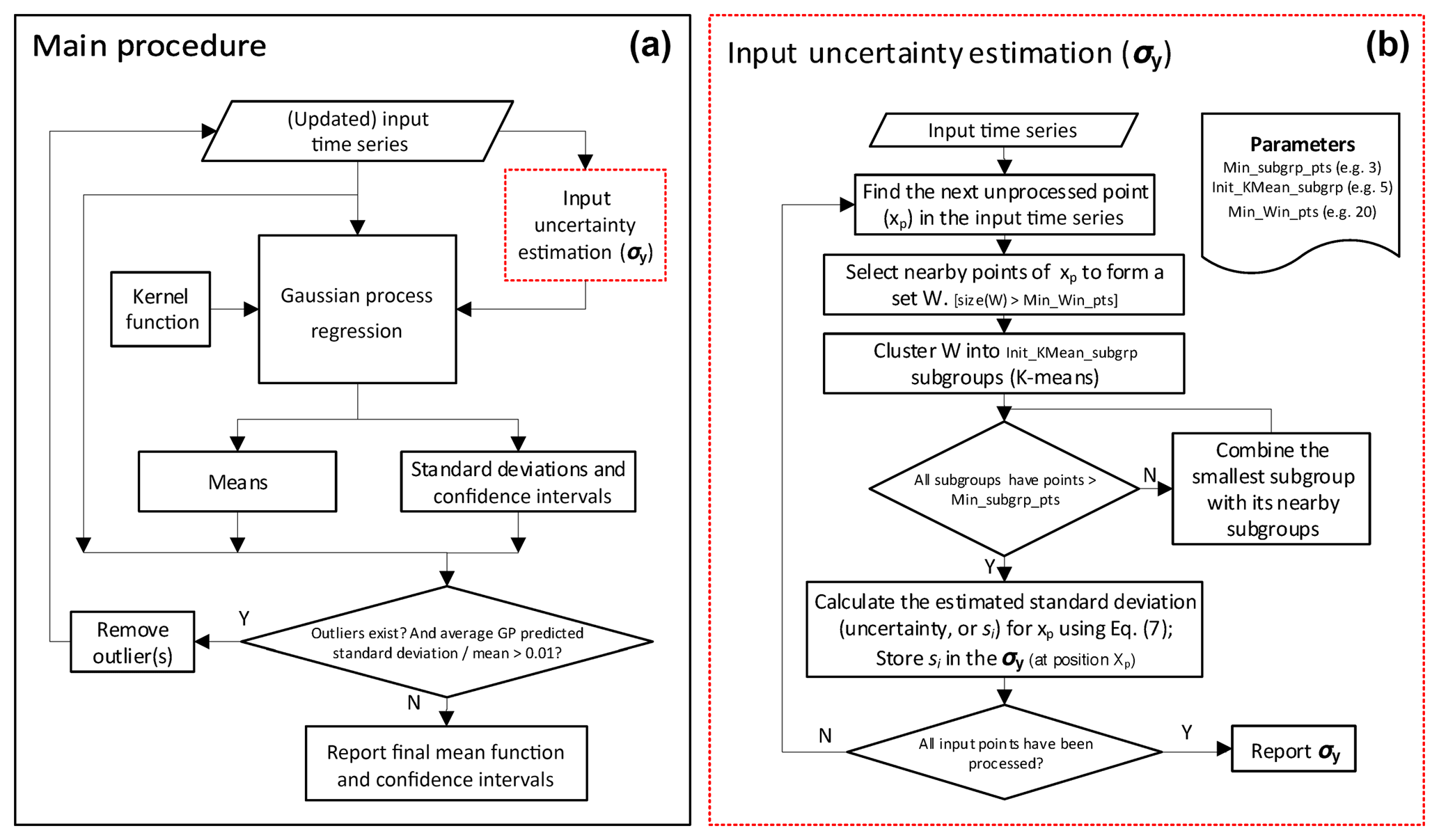
Figure 1 Main procedure for deriving the mean and confidence interval functions using Gaussian process regression (a) and detailed procedure of the proposed input uncertainty estimation method (b).

2.2 Moving average (MA)

MA is a simple smoothing technique. To assess the performance of the GP regression with other methods, this study implements MA for a one-dimensional case as follows. For a given x_*i, we first choose its nearby observations $\left\{(x,y)\left|\left|x-x_{*i}\right|\le \mathrm{win}\mathit{\_}\mathrm{size},(x,y)\in {\mathcal{D}}_{\mathrm{obs}}\right.\right\}$ within the given window win_size and then calculate the mean y value of the subset as the smoothed observation at x_*i. The process is repeated for all possible x values in 𝒟_*. The parameter win_size of MA is set at 20 for all applicable cases in this study.

2.3 UVMRP operational algorithm (OPER)

UVMRP operational algorithm (OPER) was specially designed for smoothing its in situ calibration factor sequences (http://uvb.nrel.colostate.edu/UVB/dataProcessingInfo/VnaughtsDataProcessing.jsf, last access: 8 August 2018). OPER is included as an additional source for method comparison. The algorithm has three steps. In the first step, a 12-count running mean and the corresponding standard deviation are maintained to detect outliers (i.e., points outside half of the running mean or 2 standard deviations). During the process, if three consecutive points are determined to be outliers, visual examination is performed to determine if a permanent change in the instrument responsivity has occurred. If such a change is confirmed, calculation of a new running mean begins on the three points. In the second step, a moving linear regression (LR) is used to smooth the values at the center of each moving window. The moving window size is ±3 months. If visual examination finds significant value changes on a date of interest (the center of a moving window), the regression is not performed on that date. In the final step, the regression results from step two are used as input into a weighted means algorithm to generate continuous and smooth in situ calibration factors. The inverse of year fraction between the current date of interest and the date of each participating point is used to calculate the weights. The weighting window is also ±3 months from the date of interest.

2.4 Validation method for 368 nm in situ calibration factors

Ideally, to avoid additional uncertainties caused by the interpolation among wavelengths, the calibration factors should be validated via a direct comparison of direct sun signals from the to-be-calibrated UV-MFRSR and a reference instrument measuring at the 368 nm channel (e.g., the standard precision filter radiometer (PFR) operated by the Physikalisches-Meteorologisches Observatorium Davos, World Optical Depth Research Calibration Center (WORCC)). However, such reference measurements are not available at most UVMRP stations. Therefore, the estimated mean normalized V₀ (V_0,norm) values from the GP regression and the other two comparison methods (i.e., MA and OPER) are validated indirectly in terms of aerosol optical depth (AOD) against those obtained at the collocated AERONET sites. As shown in Appendix C, the uncertainty of UV-MFRSR AODs exceeds the World Meteorological Organization (WMO) U95 criterion (e.g., 95 % of the measured data have uncertainty in the range of 0.005±0.01 per air mass; Kazadzis et al., 2018) at the UVMRP sites investigated here because the stability assumption of the Langley method may not be strictly fulfilled. Therefore, the AOD comparison in this study can only serve as indirect evidence to verify whether the calibration of UV-MFRSR is reasonably accurate. AERONET sun photometers are routinely calibrated with the uncertainty of AOD around 0.002 to 0.005 in the visible range and up to 0.01 in the UV region (Eck et al., 1999; Holben et al., 2001) and are therefore considered a reliable source for AOD intercomparison and radiometer validation (e.g., Alexandrov et al., 2002, 2008; Augustine et al., 2003; Krotkov et al., 2005a, b; Kassianov et al., 2007; Tang et al., 2013; Yin et al., 2015; Zhang et al., 2016). During the recent Fourth WMO Filter Radiometer Comparison held in Davos, Switzerland (between 28 September and 16 October 2015), most AOD values derived from the three AERONET CIMEL sun photometers are within the ±0.01 range compared with the PFR triad standard (Kazadzis et al., 2018). This includes those determined at 368 nm from the extrapolation of AERONET AODs at 340 and 380 nm. The 2015 Davos campaign also included four MFRSR instruments. Overall, the results showed good agreement among the four MFRSRs and the PFR triad standard, though one instrument exhibited a positive bias and low precision compared to the sun-pointing instruments (Kazadzis et al., 2018). However, such errors were likely explained by instrument-specific uncertainties (e.g., angular response correction, responsivity calibration, and shadowband position issues) and do not suggest inherent error in MFRSR AODs (Kazadzis et al., 2018). Augustine et al. (2003) compared SURFRAD MFRSR AODs at the Table Mountain station in Colorado with UVMRP MFRSR AODs at the Pawnee station (85 km northeast of Table Mountain) and with National Renewable Energy Laboratory (NREL) sun-photometer-derived AODs at Golden station (50 km to the south). The AOD difference in the test cases showed a magnitude of 0.1 to 0.2 and was variable over time even for the same comparison site. Krotkov et al. (2005a, b) validated the UVMRP UV-MFRSR AODs with the interpolated AERONET AODs at the 368 nm at the National Aeronautics and Space Administration Goddard Space Flight Center (NASA/GSFC) site in Greenbelt, Maryland. They found that the UV-MFRSR AODs at 368 nm channel on cloud-free days had a daily RMSE of less than 0.01 when calibrated using AERONET measurements and increased to approximately 0.02–0.05 (depending on the season) when calibrated using the standard Langley method (Harrison and Michalsky, 1994; Slusser et al., 2000). Alexandrov et al. (2002) developed a comprehensive calibration method for the VIS-MFRSR and validated the calibration at the four channels (i.e., 440, 500, 670, and 870 nm) by comparing the derived AOD values with interpolated AERONET values at the ARM Cloud and Radiation Testbed (CART) site. The results showed a small AOD difference (i.e., < 0.005) at the 440, 500, and 870 nm channels for a variety of atmospheric conditions with AODs ranging from 0.03 to 0.4 (at 500 nm). Alexandrov et al. (2008) considered optical depth of NO₂ and ozone during the MFRSR AOD calculation, although they were small enough to be ignored (i.e., 0.008 NO₂ optical depth at 415 nm and 0.005 ozone optical depth at 615 nm) at their test location at the ARM Southern Great Plains (SGP) site. The long-term intercomparison showed a good agreement (i.e., difference between them < 0.01) between the MFRSR and AERONET AODs at the 440, 675, and 870 nm channels. Kassianov et al. (2007) validated the MFRSR-retrieved optical properties and reported small RMSE values (i.e., 0.0043–0.0075) among MFRSR, AERONET, and normal incidence multifilter radiometer (NIMFR) AODs at the 500 and 870 nm channels during the ARM program's Aerosol Intensive Operational Period (IOP) in 2003.

In this study, for the UV-MFRSR at the 368 nm channel, AOD (AOD_{368 nm,UVMRP}) is calculated by subtracting Rayleigh optical depth (RLOD_{368 nm,UVMRP}) from total optical depth (TOD_368nm,UVMRP) under cloud-free conditions. The absorption of O₃, NO₂, and other trace gases is very small at the 368 nm channel (e.g., NO₂ optical depth is around 0.002 to 0.003 at AERONET Cart_Site), so they are ignored during the calculation of AOD_{368 nm,UVMRP}:

$$\begin{array}{ll}{\displaystyle }& {\displaystyle }{\mathrm{AOD}}_{\mathrm{368}\mathrm{nm},\mathrm{UVMRP}}\approx {\mathrm{TOD}}_{\mathrm{368}\mathrm{nm},\mathrm{UVMRP}}\\ \text{(8)}& {\displaystyle }& {\displaystyle }-{\mathrm{RLOD}}_{\mathrm{368}\mathrm{nm},\mathrm{UVMRP}}.\end{array}$$

TOD is calculated using Beer's law (e.g., Slusser et al., 2000), for which the actual calibration factor at the top of the atmosphere (V_0,raw) is restored from GP-estimated mean V_0,norm. The cosine-corrected voltage and air mass are obtained from the UVMRP web page (https://uvb.nrel.colostate.edu/UVB/da_queryCosCorrected.jsf, last access: 8 August 2018). RLOD is calculated by following the equations in Bodhaine et al. (1999). The site latitude and height for RLOD calculation are from the UVMRP web page (https://uvb.nrel.colostate.edu/UVB/uvb-siteinfo.jsf, last access: 8 August 2018), and the instantaneous site-level surface pressure for RLOD calculation is obtained from the collocated AERONET sites (https://aeronet.gsfc.nasa.gov/cgi-bin/webtool_opera_v2_new, last access: 31 July 2018).

To obtain reliable AOD values, UV-MFRSR measurements with quality concerns or cloud contamination are excluded in the following comparison. More specifically, (1) any measurements with UVMRP-provided quality control flag(s) relevant to the data quality of the direct beam at the 368 nm channel are excluded; (2) data with small (direct beam) measurements at 368 nm are also excluded because they are more sensitive to noise or errors introduced during various calibration steps; and (3) a simple variation check is performed to reduce the potential of mixing cloud and AOD. If the ratio between the standard deviation of TODs and the mean TOD value in the 15 min time window exceeds 0.05, they are excluded from further analyses.

AERONET (v2.0) provides AOD at the 340 and 380 nm channels. These values are interpolated to the effective wavelength of the UV-MFRSR 368 nm channel for comparison using the Ångström exponent as follows. Note that in the log-transformed coordinate system (i.e., log(AOD) vs. log(wavelength)), log(AOD) is generally linear between 340 and 380 nm (Krotkov et al., 2005a). First, the AERONET AOD spectrum between the two wavelengths is derived by linear interpolation of AERONET AODs at 340 and 380 nm in the log-transformed coordinate system. Next, since the UV-MFRSR AOD at 368 nm is a band-pass value over a narrow band (i.e 2 nm FHMW), the equivalent AERONET AOD at that channel is derived by

$$\begin{array}{}\text{(9)}& {\mathrm{AOD}}_{\mathrm{368}\mathrm{nm},\mathrm{AERONET}}={\displaystyle \frac{{\int }_{\mathrm{340}\mathrm{nm}}^{\mathrm{380}\mathrm{nm}}{\mathrm{AOD}}_{\mathit{\lambda }}{F}_{\mathit{\lambda }}\mathrm{d}\mathit{\lambda }}{{\int }_{\mathrm{340}\mathrm{nm}}^{\mathrm{380}\mathrm{nm}}{F}_{\mathit{\lambda }}\mathrm{d}\mathit{\lambda }}},\end{array}$$

where AOD_λ is the interpolated AERONET AOD spectrum, F_λ is the spectral response function of the UV-MFRSR at the 368 nm channel (http://uvb.nrel.colostate.edu/UVB/da_queryFilterFunctions.jsf, last access: 8 August 2018), and the wavelength interval for the integral is 0.05 nm. Note that negative AERONET AOD measurements are excluded from the validation because of using log transformation.

Since AERONET and UV-MFRSR AOD values at 368 nm are derived from measurements involving different instruments and wavelengths, the uncertainties when comparing these AOD values should be noted. Some important sources of uncertainties include the following.

1. AERONET calibration error. At the time of calibration at Mauna Loa Observatory, AERONET reference instruments have an uncertainty of ∼0.2 % to 0.5 %, which is equivalent to a 0.002 to 0.005 uncertainty in AERONET AOD (Holben et al., 2001). These calibration factors are likely to shift within the year following calibration, which may result in a total AOD uncertainty of ∼0.01 to 0.02 (wavelength dependent, higher in the UV) (Holben et al., 2001).

2. Instrument field of view (FOV). AERONET CIMELs have a FOV of 1.2^∘ while the UV-MFRSR has a larger FOV (e.g., ∼6.5^∘; reported by Kazadzis et al., 2018). AODs obtained from instruments with larger FOVs are associated with greater AOD uncertainty due to larger contributions of scattered light to the direct irradiance measurement (Kim et al., 2005).

3. Instrument maintenance. Periodic soiling and cleaning of the UV-MFRSR diffuser can result in spurious increases and decreases in AOD, respectively. The frequency of on-site maintenance (e.g., cleaning of the UV-MFRSR dome) as well as rainfall events may therefore account for some of the AOD difference (Kim et al., 2005, 2008).

4. Trace gases. As mentioned above, AERONET AOD accounts for NO₂ optical depth (e.g., ∼0.002–0.003 at OK02) while UV-MFRSR AOD does not.

2.5 Datasets

2.5.1 Synthetic case

We generate a synthetic time series that is composed of six segments with a varying base function and noise levels (Fig. 2a). The base function (Eq. 10), including linear, quadratic, and cubic functions, simulates a wide variety of functions for which the proposed technique is applicable. The noise levels are the same within each segment but different across segments. The noise at segment i is sampled from a fixed normal distribution $\mathcal{N}\left(\mathrm{0},{\mathit{\sigma }}_i^{\mathrm{2}}\right)$, where σ_i is equal to 4, 8, 6, 15, 7, and 3 from left to right segments. Each segment originally contains 200 points. Their x coordinates are sampled randomly from six uniform distributions within their domains. Points with x coordinates in the three designated windows (i.e., [64.2, 69.2], [80.8, 85.8], and [122.5, 127.5]) are removed to simulate data gaps in reality.

$$\begin{array}{}\text{(10)}& y=\left\{\begin{array}{ll}\mathrm{1.5}x-\mathrm{30},& \mathrm{0}\le x<\mathrm{50}\\ -\mathrm{1.2}(x-\mathrm{50})+\mathrm{45},& \mathrm{50}\le x<\mathrm{100}\\ -\mathrm{0.02}(x-\mathrm{100}{)}^{\mathrm{2}}& \mathrm{100}\le x<\mathrm{150}\\ +\mathrm{2.3}(x-\mathrm{100})-\mathrm{15},& \\ -\mathrm{0.02}(x-\mathrm{150}{)}^{\mathrm{2}}& \mathrm{150}\le x<\mathrm{200}\\ -\mathrm{0.5}(x-\mathrm{150})+\mathrm{50},& \\ \mathrm{0.0004}(x-\mathrm{200}{)}^{\mathrm{3}}& \mathrm{200}\le x<\mathrm{250}\\ +\mathrm{0.012}(x-\mathrm{200}{)}^{\mathrm{2}}& \\ +\mathrm{0.4}(x-\mathrm{200})-\mathrm{25},& \\ \mathrm{0.002}(x-\mathrm{250}{)}^{\mathrm{3}}& \mathrm{250}\le x<\mathrm{300}\\ -\mathrm{0.1}(x-\mathrm{250}{)}^{\mathrm{2}}& \\ -\mathrm{2.5}(x-\mathrm{250})+\mathrm{75},& \end{array}\right.\end{array}$$

2.5.2 Application cases: in situ calibration factors

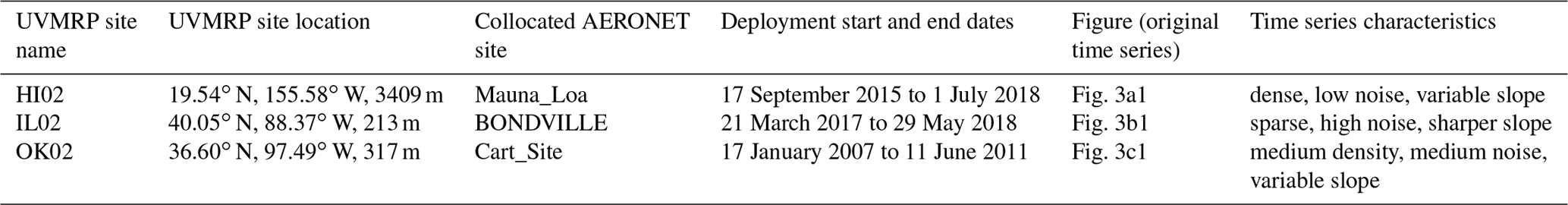
In this study, the in situ calibration factors of UVMRP UV-MFRSRs are used as application cases to test the performance of the three smoothing methods (i.e., GP, MA, and OPER). These UV-MFRSR in situ calibration factors over several months or years are obtained through the Langley method on clear days. Their varying uncertainties are mainly attributed to two aspects. One is the optical stability of atmospheric constituents (e.g., the aerosol, ozone, and thin clouds) when the in situ calibration factor is derived (Chen et al., 2015), and the other is the aging status of the radiometer. UVMRP publish its in situ calibration factors on their website (http://uvb.nrel.colostate.edu/UVB/da_queryVoIntercepts.jsf, last access: 8 August 2018). To reduce the chances of abrupt changes in the sequences, the data associated with the same instrument (i.e., UV-MFRSR) at the same UVMRP site (denoted as a deployment period) are processed together. Three UVMRP sites with collocated AERONET sites (for validation) were selected (Table 1). The in situ calibration factors at these UVMRP sites represent time series with contrasting densities, noisiness, and slopes (Table 1). Appendix B uses the Oklahoma site (OK02) to show that the UV-MFRSR 368 nm in situ calibration factors obey normal distribution.

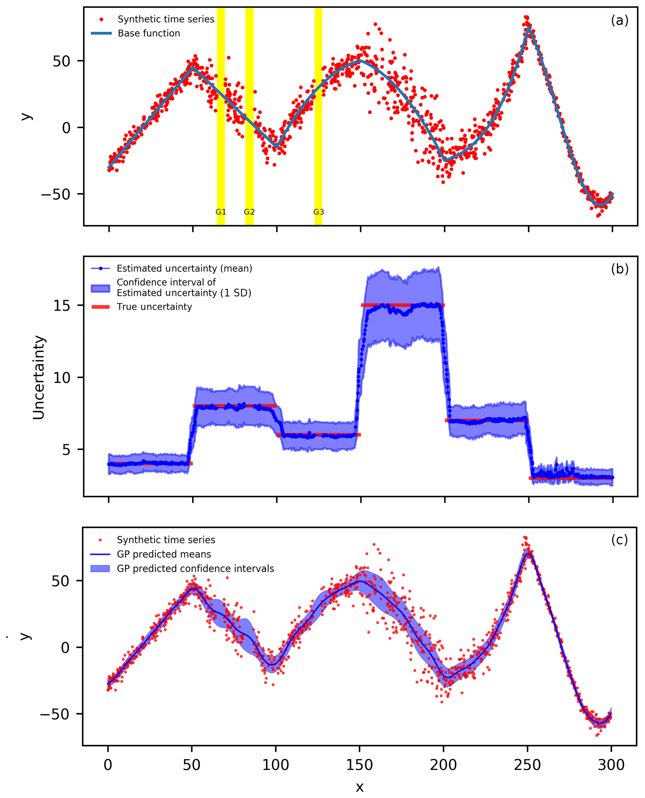
Figure 2 (a) The synthetic time series based on Eq. (10) (the blue line) with varying noise levels. There are originally 200 samples within every 50-wide interval (or segment) in the x coordinate, but points between [64.2, 69.2] (highlighted in yellow, G1), [80.8, 85.8] (highlighted in yellow, G2), and [122.5, 127.5] (highlighted in yellow, G3) are removed to simulate data gaps in practice. The final number of points in the sequence is 1140. (b) The means (dark blue circles) and confidence intervals (light blue area) of the estimated uncertainty for the 200 synthetic sequences (all sampled from the distribution of (a) but with different random noise). The true uncertainty (red line segments) is also displayed. (c) The Gaussian process regression results for the synthetic time series from (a). The dark blue line is the predicted mean function and the light blue area is the corresponding confidence intervals.

Table 1 The three UVMRP 368 nm UV-MFRSR in situ calibration factor time series for test.

3 Results and discussion

3.1 Synthetic case

3.1.1 Estimation of input uncertainty for Gaussian process

The proposed dynamic input uncertainty estimation method is first applied to the synthetic case. To observe the statistical properties and characteristics of the estimated input uncertainty, this procedure was applied to 200 synthetic time series, each of which is generated by adding random noise into the base function (Eq. 10) following the procedures discussed in Sect. 2.5.1.

Figure 2b shows the means (dark blue circles) and confidence intervals (light blue area) of estimated uncertainty of the 200 estimated input uncertainty sequences. The mean of the estimated uncertainty is close to the true uncertainty (RMSE = 0.6321) for the entire synthetic case as demonstrated by a LR between estimated and true uncertainty with a slope close to 1 (i.e., 1.0332) and a high R² of 0.9759 (Table 2). Most true uncertainty (red line segments) is covered by the confidence intervals except for the areas near the ends of the six segments. In these areas, the method averaged the uncertainty from the adjacent segments and presented a smooth transition between segments. This small RMSE value suggests that using smaller subgroup size (e.g., three to six points) does not significantly influence the estimation of uncertainty (Fig. 2a). Therefore, smaller subgroups are preferred over larger ones as larger subgroups are more likely to have gap(s) with large variation, which tends to increase its estimated standard deviation (Eq. 7).

Table 2 Validation of the input uncertainty and mean of GP prediction using four input uncertainties: the input uncertainty estimated by the proposed method (Sect. 2.1.2), overall standard deviation of the synthetic time series (30.95), minimum true uncertainty of the synthetic time series (2.00), and maximum true uncertainty of the synthetic time series (15.00). RMSE stands for root-mean-square error. LR stands for linear regression. R² stands for the coefficient of determination for linear regression.

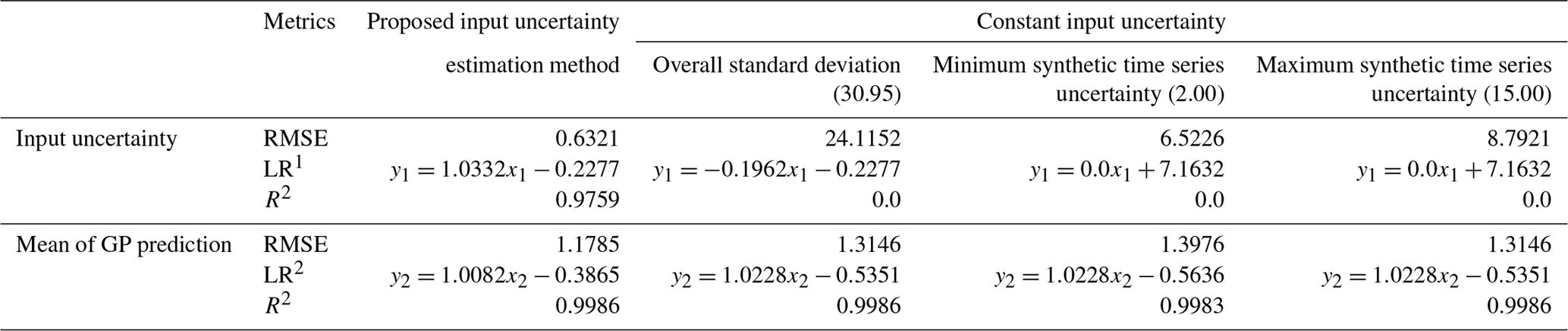
Note: ¹ y₁ represents the true input uncertainty of the synthetic time series; x₁ represents the estimated input uncertainties. ² y₂ represents the true values on the base function (Eq. 10); x₂ represents the GP-estimated mean values using the respective input uncertainty.

To demonstrate the improvements in the GP resulting from the dynamic input uncertainty estimation, the GP is also run with three typical constant input uncertainties: overall standard deviation of the synthetic time series (30.95), minimum true uncertainty of the synthetic time series (2.00), and maximum true uncertainty of the synthetic time series (15.00). The results from all three constant input uncertainties are less accurate than the estimated input uncertainty generated by the proposed method (Table 2). The proposed method has a significantly smaller RMSE (i.e., 0.6321) compared with the three constant input uncertainties (i.e., 24.1152, 6.5226, and 8.7921, respectively). Similarly, the LR between the estimated and true uncertainties shows that the proposed method has slope and R² values both close to 1 (i.e., 1.0332 and 0.9759) while the three constant uncertainties show no (linear) correlation with true uncertainties (i.e., the slope and R² values close to zero).

3.1.2 Estimation of means and confidence interval and its validation

The kernel function in the GP regression used in this study is the RQ kernel, with two parameters: length scale and alpha (Eq. 2). To use RQ with GP regression, we need to provide the initial (estimated) values for these two parameters. First, we round the original data points (red points in Fig. 2a) to the nearest 0.25 interval grids. Then, we calculate the autocorrelation on these rounded data points from lags of 0.25 to 22.25 (approximately equivalent to lags of 1 to 90 points). Next, we perform curve fitting on autocorrelation results and obtain 9.80 and 1.05 as initial length scale and alpha estimates, respectively. With these initial RQ parameters and the estimated input uncertainty (from the proposed method or using three representative constant input uncertainties), GP regression predicts the mean and uncertainty functions. Figure 2c shows the GP results for the proposed method: dark blue line for the mean function and the light blue area for the confidence intervals (4.42 times of the GP-predicted uncertainty function).

In terms of the GP-predicted mean function vs. the base function (Eq. 10), the proposed input uncertainty estimation method shows a 12.0 % to 15.7 % improvement on RMSE over the three constant input uncertainties (i.e., 1.1785 vs. 1.3146, 1.3976, and 1.3146) (Table 2). Similarly, the slope of the LR between the two functions is closer to 1 for the proposed uncertainty estimation method (i.e., 1.0082) than the three constant uncertainties (i.e., 1.0228). In addition, the predicted mean function from the proposed method is close to the base function even near the gaps (G1, G2, and G3 in Fig. 2a, c). Additionally, the proposed method's predicted uncertainty function (or confidence intervals) shows better agreement with the true uncertainty of the synthetic time series (Fig. 2c) while the three constant input uncertainties' results show a consistent over- or underestimated pattern over the entire time series (figures not shown). It is noted that the predicted confidence intervals from the proposed method are wider near the three gaps (G1, G2, and G3 in Fig. 2a) than nearby locations with similar uncertainty. This is anticipated because the constraint in the gaps are from distant points at which the RQ kernel gives low correlation.

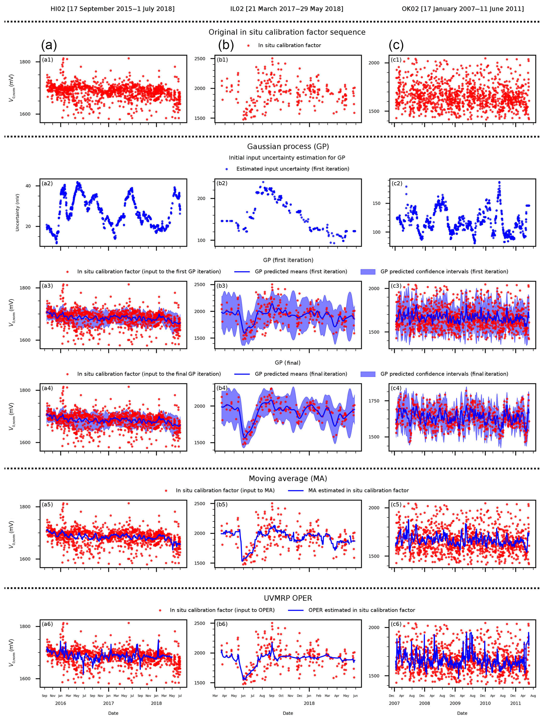
Figure 3 The results of the three smoothing methods (i.e., GP – Gaussian process; MA – moving average; OPER – UVMRP operational algorithm) for the three UVMRP in situ calibration factor sequences: (a) HI02 (17 September 2015 to 1 July 2018), (b) IL02 (21 March 2017 to 29 May 2018), and (c) OK02 (17 January 2007 to 11 June 2011). Panels (a1), (b1), (c1) display the original in situ calibration factor (V_0,norm) sequence. Panels (a2), (b2), (c2) show the initial input uncertainty estimated for GP. Panels (a3), (b3), (c3) present the predicted daily mean and confidence interval from the first iteration of GP. Panels (a4), (b4), (c4) show the final results of GP after iterations. Panels (a5), (b5), (c5) show the results of MA. Panels (a6), (b6), (c6) show the results of OPER.

3.2 In situ calibration factors cases

3.2.1 Applications

The same GP procedure is applied to three in situ calibration factor (V_0,norm, sun-earth distance normalized) sequences from three UVMRP deployment periods (Fig. 3) at three different UVMRP locations previously described in Table 1.The Hawaii site (HI02) sits at a clean, high-altitude location, which means its atmospheric condition is more stable than other UVMRP sites and its V_0,norm has the lowest variation (Fig. 3a1). The Illinois site (IL02) is surrounded by croplands/rangelands with the closest city (Champaign) located 12 km northwest (Fig. 3b1). The Oklahoma site (OK02) is also surrounded by croplands/rangelands with the closest city (Oklahoma City) located about 96 km south (Fig. 3c1). Both wildfires and agricultural activities (e.g., cultivation and harvest) at IL02 and OK02 contribute to the relatively hazy and unstable atmosphere condition for Langley regression. As a result, V_0,norm values at IL02 and OK02 have larger variation compared with HI02. The dynamic input uncertainty estimation results confirm that the uncertainty at HI02 (15–40; Fig. 3a2) is also lower than at the other two sites (100–300; Fig. 3b2, c2). Generally, the proposed method gives lower uncertainty values for time windows with more clustered points (e.g., December 2008 and April 2010 at OK02, Fig. 3c2; February 2017 at HI02, Fig. 3a2). There are no obvious temporal patterns of uncertainty at any of the three sites.

Figure 3a3, b3, and c3 show the estimated means (dark blue line) and confidence intervals (light blue area) after the initial pass through GP. The length scale parameters of the RQ kernel for the HI02, IL02, and OK02 sites are 6.091, 6.369, and 6.228 (days), respectively. Their corresponding alpha parameters of the RQ kernel function are all close to 1.0 (i.e., 0.948, 0.862, and 0.944, respectively). As expected, the confidence interval is narrower near time windows with more data points, and the confidence intervals are wider near gaps (Fig. 3b3).

As depicted in Fig. 1, the outlier removal and GP are repeated following the initial GP regression, giving the final GP results shown in Fig. 3a4, b4, and c4. After this final pass, the length scale parameters of the RQ kernel function for the HI02, IL02, and OK02 sites are 6.091, 11.149, and 6.907 (days), respectively. Compared with the first round, all length scale parameters increase as more outliers are removed (except for HI02). At HI02, the average ratio between GP means and standard deviations is lower than the threshold (i.e., 0.01) after the first round and the iteration stops. The corresponding alpha parameters of the RQ kernel function are still all close to 1.0 (i.e., 0.948, 1.010, and 1.110, respectively). Because of outlier removal, compared with the first-round results, GP generates smoother mean functions and narrower confidence intervals at the last round.

Figure 4 The 368 nm AOD scatter plots between UVMRP (y axis) and AERONET (x axis). The UVMRP 368 nm AODs are calculated from UV-MFRSR direct normal voltages using calibration factors estimated by the three methods (i.e., from top to bottom: GP, MA, OPER) at the three sites (i.e., from left to right: HI02, IL02, OK02). Panels (a), (b), and (c) display the scatter plots for the GP method at HI02, IL02, and Ok02, respectively. Similarly, panels (c), (c), and (f) are for the MA method and panels (g), (h), and (i) are for the OPER method. The AERONET 368 nm AODs are derived from collocated (i.e., Mauna_Loa, BONDVILLE, Cart_Site) AERONET AODs on the 340 and 380 nm channels. The linear regression line (solid, red) and the 1-by-1 line (dashed, black) are also plotted. “< y−x >” means the average difference between AERONET and UVMRP AOD at the 368 nm channel. “SD(y−x)” means the standard deviation of their difference.

The other two methods (i.e., MA and OPER) are applied to the same in situ calibration time series. They can provide mean functions but not confidence intervals. The MA (win_size =20) results (Fig. 3a5, b5, and c5) are generally smoother than OPER (Fig. 3a6, b6, and c6) but both are more responsive to noisy points than GP. In addition, since OPER is scheduled to run once per month on active deployments, there may be some lags at the end of those deployments (e.g., Fig. 3a6).

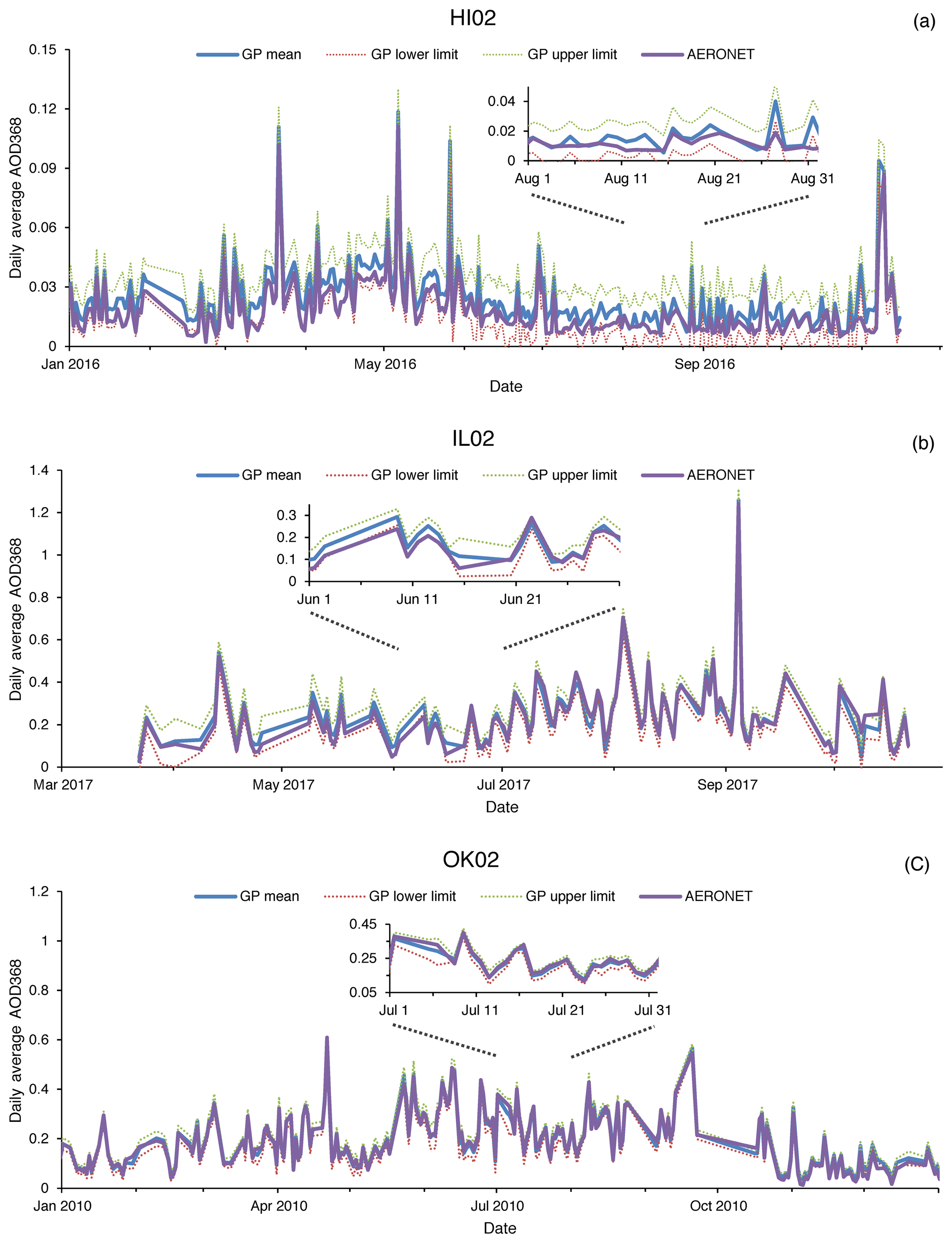
Figure 5 Time series of UVMRP and AERONET 368 nm daily average AOD at the HI02, IL02, and OK02 sites. The daily AOD mean values derived from the GP mean in situ calibration factor (V₀) functions (blue) and the corresponding AERONET values (purple) are shown as solid blue lines. The corresponding lower and upper limits of AOD derived from the GP V₀ confidence intervals are shown as dotted red and green lines, respectively. The insets for HI02 (August 2016), IL02 (June 2017), and OK02 (July 2010) are also included in the respective subplots to show the comparison details.

3.2.2 Validation

Following the procedures described in Sect. 2.4, the UVMRP AODs at the 368 nm channel generated by GP, MA, and OPER are validated against the corresponding AERONET AODs at the three collocated sites (i.e., HI02 – Mauna_Loa, IL02 – BONDVILLE, OK02 – Cart_ Site). The scatter plots between these UVMRP and AERONET AODs are displayed in Fig. 4. The performance of all three methods at HI02 (Fig. 4a, d, g) are similar. For example, the average bias “< y−x >” is approximately 0.0054 and standard deviation of the difference “SD(y−x)” is approximately 0.0066. For IL02 (Fig. 4b, e, h) and OK02 (Fig. 4c, f, i), GP shows superior agreements with AERONET to that of the other two methods. For example, at IL02, the absolute value of GP's average bias (0.0036) is about 3.3 to 2.5 times lower than that of MA (0.0119) and OPER (0.0091). Similarly, at OK02, the average bias for GP (0.0032) is much lower than that for MA (0.0119) and OPER (0.0087). The validation results for GP at OK02 are similar to the previous comparison results between AERONET and MFRSR AODs at 415 and 440 nm (Tang et al., 2013; Alexandrov et al., 2008). Furthermore, as shown in Appendix C, the GP method improves agreement between UVMRP and AERONET 368 nm AOD across all air masses.

Table 3 Statistical metrics (average absolute difference, average absolute relative difference, and linear regression) on comparing 368 nm AOD between UVMRP (AOD_368,UVMRP) and AERONET (AOD_368,AE). The UVMRP 368 nm AODs at the three sites (i.e., HI02, IL02, and OK02) are calculated using calibration factors estimated using the three methods (i.e., GP, MA, and OPER). The AERONET 368 nm AODs are derived from collocated (i.e., Mauna_Loa, BONDVILLE, and Cart_Site) AERONET AODs on the 340 and 380 nm channels. LR stands for linear regression. R² stands for the coefficient of determination for linear regression. The “x” and “y” in LR refer to AOD_368,AE and AOD_368,UVMRP of the respective methods.

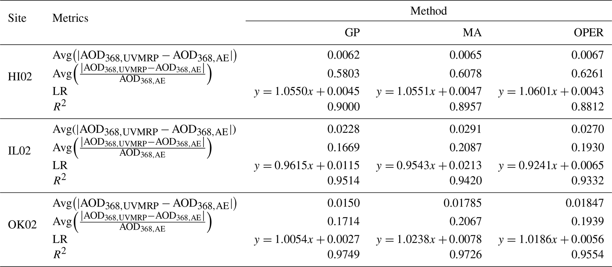
Table 3 shows two additional statistical metrics for validation: “Avg($|{\mathrm{AOD}}_{\mathrm{368},\mathrm{UVMRP}}-{\mathrm{AOD}}_{\mathrm{368},\mathrm{AE}}|$)”, a measure of absolute difference between the two quantities and “Avg($|{\mathrm{AOD}}_{\mathrm{368},\mathrm{UVMRP}}-{\mathrm{AOD}}_{\mathrm{368},\mathrm{AE}}|/{\mathrm{AOD}}_{\mathrm{368},\mathrm{AE}}$)” a measure of relative difference between the two quantities. For HI02, the GP V_0,norm values improve both the absolute and relative differences between AOD_368,UVMRP and AOD_368,AE when compared to MA (by ∼4.5 %) and OPER AODs (by ∼7.5 %), respectively. Results from LRs performed between AOD_368,UVMRP and AOD_368,AE are also reported in Table 3. The LR results are similar between GP and MA, but GP has a LR slope closer to 1 (1.0550) and higher R² (0.9000) than those of OPER (1.0601 and 0.8812) for HI02. For IL02, GP shows 21.6 % smaller absolute difference and 20.0 % smaller relative difference to AERONET than MA; GP shows 15.6 % smaller absolute difference and 13.5 % smaller relative difference to AERONET than OPER. Similarly, for OK02, GP shows 16.0 % smaller absolute difference and 17.1 % smaller relative difference to AERONET than MA; GP shows 18.8 % smaller absolute difference and 11.6 % smaller relative difference to AERONET than OPER.

Overall, the 368 nm AODs by GP show higher correlation, closer to 1 slopes, and lower absolute and relative biases compared to AERONET AODs than MA and OPER at all three sites. The improvement of GP over MA and OPER at IL02 and OK02 is more significant than at HI02. The main reason may be that HI02 is the least polluted site among the three sites. Both of its maximum and mean 368 nm AOD values are low: 0.35 and 0.016, respectively. As a result, higher accuracy of Rayleigh and other optical depth components is required to discern small improvement in AOD for HI02. Since AERONET's sun photometer is routinely calibrated, the agreement on AOD values suggests that the calibration factor mean functions generated by GP are more accurate than those of MA and OPER.

In addition, Fig. 5 shows the 368 nm AOD time series calculated using GP-generated in situ calibration factors at the three UVMRP sites. The blue solid line represents the AODs calculated using the GP means, and the green and red dotted lines represent the AODs calculated using the GP confidence intervals. It is seen that the AOD confidence intervals are approximately ±0.0095, ±0.0480, and ±0.0273 at HI02, IL02, and OK02, respectively. The corresponding AERONET AOD time series are also plotted (i.e., purple lines in Fig. 5). The insets in Figure 5 show comparison details at HI02, IL02, and OK02. For most of the AOD time series, AERONET results are within the GP confidence intervals. The average absolute differences of daily AOD values between GP and AERONET are ∼0.006 for HI02, ∼0.024 for IL02, and ∼0.014 for OK02. These values are close to or within the AERONET AOD uncertainty level (i.e., 0.01), suggesting the high quality of the potential UVMRP AOD product. In addition, unlike the obvious seasonal changes in AOD difference reported in the previous study at the NASA/GSFC site by Krotkov et al. (2005a), this study (Fig. 5) shows no discernible seasonal pattern in the AOD differences at all three sites.

4 Conclusions

A new dynamic uncertainty estimation method for noisy time series is developed in this study. Combining this method with Gaussian process regression, we provide a solution to estimate the underlying mean and uncertainty functions of time series with variable mean, noise, sampling density, and length of gaps. For the synthetic case with linear, quadratic, and cubic base functions; a noise level varying from 2 to 15; and noticeable gaps, the proposed solution returns a mean function with the RMSE of 1.1785 (linear regression R² of 0.9986), which is at least 12.0 % lower than RMSEs associated with the three constant input uncertainties. Its estimated input uncertainties determined by this method are close to the true uncertainty levels except for the transitional region between segments. The solution also gives accurate mean values at the three gaps. The proposed GP solution as well as the other two comparison methods (i.e., MA and OPER) were then applied to three in situ calibration factor time series of UV-MFRSR (368 nm) at three UVMRP sites. The GP solution handles the variation in slope, noise, sampling density, and length of gap in the three cases as expected. Since irradiance at 368 nm is not measured by a collocated (and calibrated) radiometer, the performance of the three methods is validated against the collocated AERONET sites in terms of AOD. The results show that AODs calculated using GP-derived UV-MFRSR calibration factors (V_0,norm) have consistently better agreement with AERONET AODs than MA and OPER in terms of average absolute and relative differences and linear regression R² values. These results suggest that the proposed GP solution is a robust method for time series analyses of data with variable mean, noise, sampling density, and length of gap and has potential for application across disciplines.

Appendix A: The formulation between the overall standard deviation and the subgroup standard deviation

Given a time series {x_i}, its total N points are divided into J groups $\mathit{\left\{}{x}_k^j\mathit{\right\}}$, and the number of points in group j is N_j (j=1, 2, … , J; k=1, 2, … , N_j). For data points in each group, their sample mean and standard deviation are μ_j and s_j. For the entire time series, its sample mean is $\mathit{\mu }=\frac{\mathrm{1}}{N}\sum _{i=\mathrm{1}}^N{x}_{\mathrm{i}}$, and the sample variance is

$$\begin{array}{ll}{\displaystyle }{s}^{\mathrm{2}}& {\displaystyle }={\displaystyle \frac{\mathrm{1}}{N-\mathrm{1}}}\sum _{j=\mathrm{1}}^J\sum _{k=\mathrm{1}}^{N_j}(x_k^j-\mathit{\mu }{)}^{\mathrm{2}}\\ {\displaystyle }& {\displaystyle }={\displaystyle \frac{\mathrm{1}}{N-\mathrm{1}}}\sum _{j=\mathrm{1}}^J\sum _{k=\mathrm{1}}^{N_j}\left[\right(x_k^j-{\mathit{\mu }}_j)+({\mathit{\mu }}_j-\mathit{\mu }){]}^{\mathrm{2}}\\ {\displaystyle }& {\displaystyle }={\displaystyle \frac{\mathrm{1}}{N-\mathrm{1}}}\sum _{j=\mathrm{1}}^J\sum _{k=\mathrm{1}}^{N_j}(x_k^j-{\mathit{\mu }}_j{)}^{\mathrm{2}}+{\displaystyle \frac{\mathrm{1}}{N-\mathrm{1}}}\sum _{j=\mathrm{1}}^J\sum _{k=\mathrm{1}}^{N_j}({\mathit{\mu }}_j-\mathit{\mu }{)}^{\mathrm{2}}\\ {\displaystyle }& {\displaystyle }+{\displaystyle \frac{\mathrm{2}}{N-\mathrm{1}}}\sum _{j=\mathrm{1}}^J\sum _{k=\mathrm{1}}^{N_j}(x_k^j-{\mathit{\mu }}_j)({\mathit{\mu }}_j-\mathit{\mu })\\ {\displaystyle }& {\displaystyle }={\displaystyle \frac{\mathrm{1}}{N-\mathrm{1}}}\sum _{j=\mathrm{1}}^J{N}_j{s}_j^{\mathrm{2}}+{\displaystyle \frac{\mathrm{1}}{N-\mathrm{1}}}\sum _{j=\mathrm{1}}^J{N}_j({\mathit{\mu }}_j-\mathit{\mu }{)}^{\mathrm{2}},\end{array}$$

where the third term on the right-hand side is equal to zero because $\sum _{k=\mathrm{1}}^{N_j}\left(x_k^j-{\mathit{\mu }}_j\right)=\mathrm{0}$ (i.e., ${\mathit{\mu }}_j=\frac{\mathrm{1}}{N_j}\sum _{k=\mathrm{1}}^{N_j}{x}_k^j$). If we assume that the sample standard deviation of each data point is invariant (i.e., $s_{\mathrm{1}}=s_{\mathrm{2}}=\mathrm{\cdots }=s_J=\widehat{s}$), then

$${\displaystyle }{s}^{\mathrm{2}}={\displaystyle \frac{N-J}{N-\mathrm{1}}}{\widehat{s}}^{\mathrm{2}}+{\displaystyle \frac{\mathrm{1}}{N-\mathrm{1}}}\sum _{j=\mathrm{1}}^J{N}_j({\mathit{\mu }}_j-\mathit{\mu }{)}^{\mathrm{2}}.$$

Appendix B: The distribution of the 368 nm in situ calibration factors of UV-MFRSR

Since the true 368 nm in situ calibration factors are not available, their distribution is derived using the AERONET 368 nm AOD distribution via Beer's law (transformed Langley regression).

Beer's law links the irradiance (or voltage, V) at the top of the atmosphere with the one that reaches the ground at time t with the equation $V_t=V_{\mathrm{0}}{e}^{-{\mathrm{TOD}}_t\cdot m_t}$, where m_t is the air mass at time t and TOD_t is the corresponding total optical depth. For the 368 nm channel, AOD is the main contributor for the TOD variation. Therefore, for a short time period, TOD_t can be expressed as the sum of a constant optical depth ($\stackrel{\mathrm{‾}}{P}$) and variable residual AOD ($\mathrm{\Delta }{\mathrm{AOD}}_t={\mathrm{AOD}}_t-\stackrel{\mathrm{‾}}{\mathrm{AOD}}$): TOD${}_t=\stackrel{\mathrm{‾}}{P}+\mathrm{\Delta }{\mathrm{AOD}}_t$. Deriving an unbiased V₀ using the Langley regression (in the transformed lnV ⋅ m⁻¹ vs. m⁻¹ coordinate system) requires the participating measurements to have a constant TOD_t over the calibration period and lnV₀ is the slope of the regression. The variation in ΔAOD_t as a linear function of the component vary linearly with $m_t^{-\mathrm{1}}$ (Chen et al., 2014). Therefore, we decompose ΔAOD_t as the sum of a constant term (α) and a $m_t^{-\mathrm{1}}$ term ($\mathit{\beta }{m}_t^{-\mathrm{1}}$), where α and β are obtained from daily AERONET 368 nm AOD measurements via linear regression. With the TOD_t components expanded, the original Beer's law equation is expressed as $\ln V_t\cdot m_t^{-\mathrm{1}}=-\left(\stackrel{\mathrm{‾}}{P}+\mathit{\alpha }\right)+\left(\ln V_{\mathrm{0}}-\mathit{\beta }\right)m_t^{-\mathrm{1}}$ and the (transformed) Langley regression obtains the slope ($\ln \stackrel{\mathrm{̃}}{V_{\mathrm{0}}}=\ln V_{\mathrm{0}}-\mathit{\beta }$) via linear regression. The disturbed distribution of $\stackrel{\mathrm{̃}}{V_{\mathrm{0}}}$ is the same as the distribution of exp (ln V₀−β). Assuming the true V₀ is 1500 mV (a typical value at OK02) and using a long-term set of β values from AERONET at Cart_Site (17 January 2007 to 11 June 2011), a set of $\stackrel{\mathrm{̃}}{V_{\mathrm{0}}}$ is obtained. Removing the tails on the distribution of $\stackrel{\mathrm{̃}}{V_{\mathrm{0}}}$ (i.e., $\stackrel{\mathrm{̃}}{V_{\mathrm{0}}}\mathit{<}\mathrm{1200}$ or $\stackrel{\mathrm{̃}}{V_{\mathrm{0}}}\mathit{>}\mathrm{1800}$), the normal test of the $\stackrel{\mathrm{̃}}{V_{\mathrm{0}}}$ set (using the Python function scipy.stats.normaltest (D'Agostino and Pearson, 1973)) returns the p value of 0.4689, which is greater than the threshold (10⁻³), suggesting that the $\stackrel{\mathrm{̃}}{V_{\mathrm{0}}}$ set comes from a normal distribution.

Appendix C: Comparison of UVMRP and AERONET 368 nm AOD differences as a function of air mass among the three methods

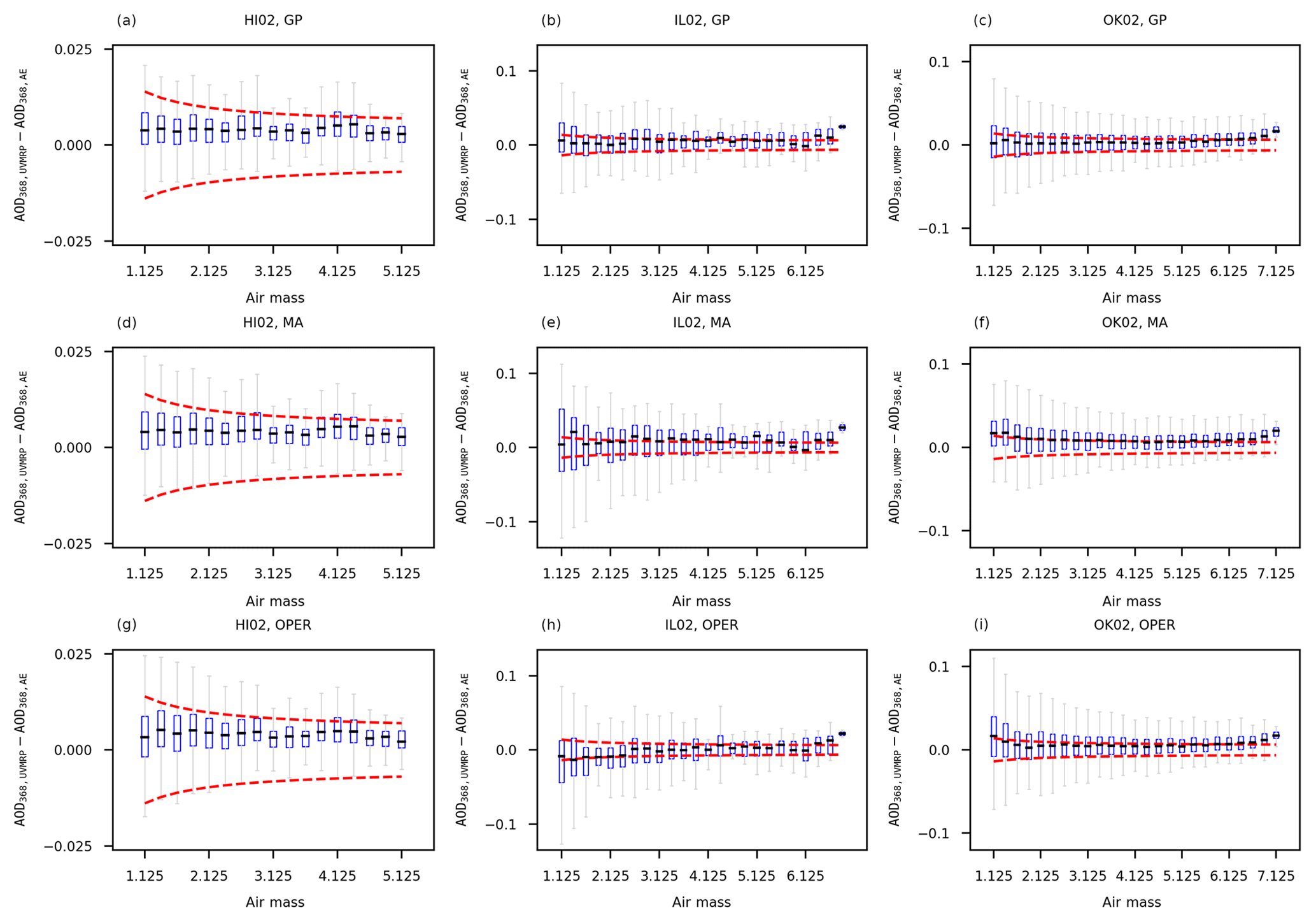
Figure C1 Box-and-whisker plots of ${\mathrm{AOD}}_{\mathrm{368},\mathrm{UVMRP}}-{\mathrm{AOD}}_{\mathrm{368},\mathrm{AE}}$ as a function of air mass by the three methods (i.e., from top to bottom: GP, MA, OPER) at the three test sites (i.e., from left to right: HI02, IL02, OK02). Panels (a), (b), and (c) display the box-and-whisker plots for the GP method at HI02, IL02, and OK02, respectively. Similarly, panels (d), (e), and (f) are for the MA method and panels (g), (h), and (i) are for the OPER method. Each blue bin covers a 0.25 air mass range. The dashed red lines show the WMO AOD U95 upper and lower limits.

Figure C1 showed that GP had narrower error ranges compared with the other two methods (i.e., MA and OPER) at all three test sites (i.e., HI02, IL02, and OK02). The median values (the short black lines in blue boxes) of GP are closer to zero at IL02 and OK02 sites, especially for lower air masses. However, regardless of site, air mass, and method, the difference between AERONET and UV-MFRSR AODs still exceeds the WMO AOD U95 criterion for a number of instances.