the Creative Commons Attribution 4.0 License.
the Creative Commons Attribution 4.0 License.
 | 03 Jun 2020
Towards spaceborne monitoring of localized CO2 emissions: an instrument concept and first performance assessment
David Krutz
Jonas Wilzewski
Carsten Paproth
Ilse Sebastian
Kevin R. Gurney
Jianming Liang
Anke Roiger
André Butz
The UNFCCC (United Nations Framework Convention on Climate Change) requires the nations of the world to report their carbon dioxide (CO2) emissions. The independent verification of these reported emissions is a cornerstone for advancing towards the emission accounting and reduction measures agreed upon in the Paris Agreement. In this paper, we present the concept and first performance assessment of a compact spaceborne imaging spectrometer with a spatial resolution of 50×50 m2 that could contribute to the “monitoring, verification and reporting” (MVR) of CO2 emissions worldwide. CO2 emissions from medium-sized power plants (1–10 Mt CO2 yr−1), currently not targeted by other spaceborne missions, represent a significant part of the global CO2 emission budget. In this paper we show that the proposed instrument concept is able to resolve emission plumes from such localized sources as a first step towards corresponding CO2 flux estimates.
Through radiative transfer simulations, including a realistic instrument noise model and a global trial ensemble covering various geophysical scenarios, it is shown that an instrument noise error of 1.1 ppm (1σ) can be achieved for the retrieval of the column-averaged dry-air mole fraction of CO2 (XCO2). Despite a limited amount of information from a single spectral window and a relatively coarse spectral resolution, scattering by atmospheric aerosol and cirrus can be partly accounted for in the XCO2 retrieval, with deviations of at most 4.0 ppm from the true abundance for two-thirds of the scenes in the global trial ensemble.
We further simulate the ability of the proposed instrument concept to observe CO2 plumes from single power plants in an urban area using high-resolution CO2 emission and surface albedo data for the city of Indianapolis. Given the preliminary instrument design and the corresponding instrument noise error, emission plumes from point sources with an emission rate down to the order of 0.3 Mt CO2 yr−1 can be resolved, i.e., well below the target source strength of 1 Mt CO2 yr−1. This leaves a significant margin for additional error sources, like scattering particles and complex meteorology, and shows the potential for subsequent CO2 flux estimates with the proposed instrument concept.
- Article
(11660 KB) - Full-text XML
-
Supplement
(290 KB) - BibTeX
- EndNote


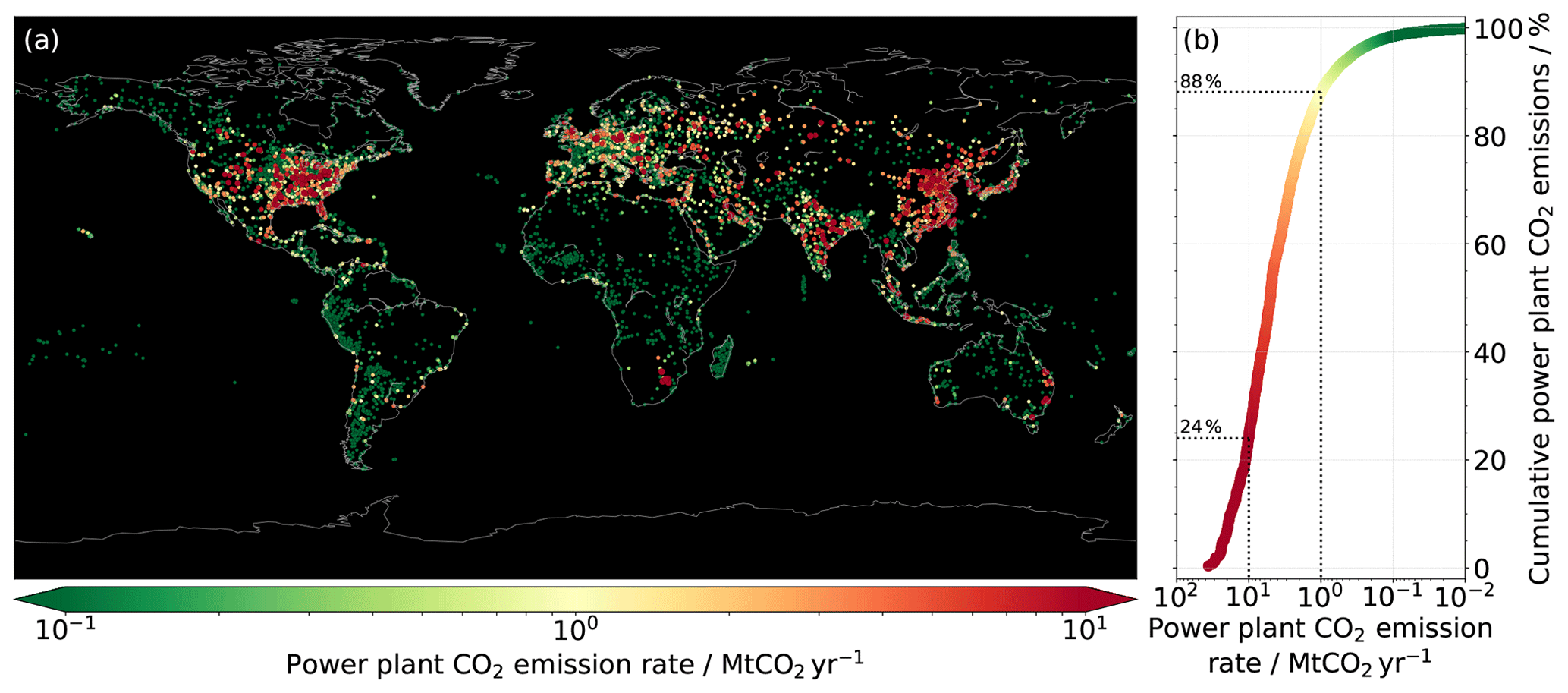
Figure 1(a) Geographical distribution of reported and estimated annual CO2 emissions from power plants worldwide for the year 2009, as provided by the CARMA v3.0 database. (b) Corresponding cumulative distribution showing the fraction of the power plant emission total (9.9 Gt CO2 yr−1) that power plants with a source strength greater than X Mt CO2 yr−1 make up. This should be understood as the fraction of the power plant CO2 emission total that can theoretically be observed by an instrument with a given sensitivity. For visualization purposes, the marker sizes in (a) are scaled according to the respective emission rates.
Despite the broad consensus on the negative long-term effects of carbon dioxide (CO2) emissions and the efforts to reduce these emissions, the atmospheric CO2 concentrations continue to rise. During the course of 2018, the average CO2 concentration increased from 407 to 410 ppm at the Mauna Loa observatory, representing the fourth-highest annual growth ever recorded at that observatory (NOAA, 2019). CO2 emissions from localized point sources represent a large fraction of the CO2 emitted into the atmosphere. The International Energy Agency (IEA) recently reported that emissions from coal-fired power plants exceeded 10 Gt CO2 yr−1 for the first time in 2018, hence accounting for approximately 30 % of the global CO2 emissions (IEA, 2019), mainly due to the continued growth of coal use in Asia and other emerging economies. Figure 1 depicts the global distribution of reported and estimated annual CO2 emissions from power plants for the year 2009, as provided by the CARMA (Carbon Monitoring for Action) v3.0 database (Wheeler and Ummel, 2008; Ummel, 2012), together with the corresponding cumulative distribution of the power plant emissions. The emission total from 16 898 individual power plants, where exact or approximate coordinates are available, adds up to 9.9 Gt CO2 yr−1. A large fraction of power plant emissions originates from a relatively small number of large to medium-sized power plants. The CARMA data show that 153 large power plants (>10 Mt CO2 yr−1) accounted for 24 % of the total annual power plant CO2 emissions, whereas 2111 large and medium-sized power plants (>1 Mt CO2 yr−1) accounted for as much as 88 % of the power plant CO2 emission budget, clearly demonstrating the significant contribution from medium-sized power plants (1–10 Mt CO2 yr−1) to the global CO2 emission budget.
To advance towards emission accounting and reduction measures, agreed upon in the Paris Agreement in force since 2016, the independent verification of reported emissions is of high importance. To this end, spaceborne instruments provide a suitable platform with which continuous long-term measurements can potentially be combined with near-global coverage with no geopolitical boundaries.
Most of the currently operating, planned and proposed instruments for passive CO2 observations from space measure the reflected shortwave infrared (SWIR) solar radiation in several spectral windows covering the oxygen A (O2 A) band near 750 nm as well as the weak and strong CO2 absorption bands near 1600 and 2000 nm, respectively, e.g., GOSAT (Greenhouse Gases Observing Satellite; Kuze et al., 2009, 2016), OCO-2 (Orbiting Carbon Observatory-2; Crisp et al., 2004, 2017), TanSat (Liu et al., 2018), GOSAT-2 (Nakajima et al., 2012), OCO-3 (Eldering et al., 2019), MicroCarb (Buil et al., 2011), GeoCarb (Moore et al., 2018), CarbonSat (Bovensmann et al., 2010; Buchwitz et al., 2013) and G3E (Geostationary Emission Explorer for Europe; Butz et al., 2015). These instruments and instrument concepts further rely on a comparatively high spectral resolution on the order of approximately 0.05–0.3 nm, representing resolving powers (ratio of wavelength over the full-width half-maximum of the instrument spectral response function) ranging from approximately 3600 for the strong CO2 absorption bands near 2000 nm for CarbonSat (Buchwitz et al., 2013) up to >20 000 for the OCO and GOSAT instruments. Such advanced instruments, like GOSAT and OCO-2 that have been operating since 2009 and 2014, respectively, generally target an accuracy and coverage sufficient to study the natural CO2 cycle on a regional to continental scale (e.g., Guerlet et al., 2013; Maksyutov et al., 2013; Parazoo et al., 2013; Eldering et al., 2017; Chatterjee et al., 2017; Liu et al., 2017) but have also been used to observe and quantify CO2 gradients on the regional scale caused by anthropogenic CO2 emissions in urban areas (Kort et al., 2012; Hakkarainen et al., 2016; Schwandner et al., 2017; Reuter et al., 2019). OCO-2 data have further been used to observe strong CO2 plumes from localized natural and anthropogenic CO2 sources like volcanoes and coal-fired power plants (Nassar et al., 2017; Schwandner et al., 2017; Reuter et al., 2019), demonstrating the capabilities of imaging spectrometers to monitor CO2 from space. The spatial resolution of OCO-2 and similar instruments like OCO-3, TanSat and the planned Copernicus CO2 Monitoring mission CO2M (on the order of 2–4 km2) does, however, pose a difficulty for the routine monitoring of localized power plant CO2 emissions, since the plume is usually only sampled by a handful of pixels in which CO2 plume enhancements cannot be fully separated from the background, making quantitative CO2 emission rate estimates difficult and vulnerable to cloud contamination and instrument noise propagating into CO2 retrieval errors. For this reason CO2M will target isolated large power plants (≳10 Mt CO2 yr−1) and large urban agglomerations (≳ Berlin) (Kuhlmann et al., 2019), and thus a large fraction of the emission total will be missed.
To contribute to closing this gap and expanding on future CO2 monitoring from space, we present the concept and a first performance assessment of a spaceborne imaging spectrometer that could be deployed for the dedicated monitoring of localized CO2 emissions. By targeting power plants with an annual emission rate down to approximately 1 Mt CO2 yr−1, a substantial fraction of the CO2 emissions from power plants and hence a significant part of the global man-made CO2 emission budget in total could be resolved (given global coverage through a fleet of instruments). As shown in Fig. 1, it is of key importance to also cover medium-sized power plants (1–10 Mt CO2 yr−1) as they alone contributed to approximately 64 % of the CO2 emissions from power plants in 2009 according to the CARMA v3.0 data. To achieve this, the proposed instrument has an envisaged spatial resolution of 50×50 m2. With such a high spatial resolution and large amount of ground pixels per unit area, averaging plume enhancements and background concentration fields is avoided. This leads to an enhanced contrast compared to a coarser spatial resolution. To increase the number of collected photons and hence the signal-to-noise ratio (SNR) and relative precision of the CO2 concentration retrievals, such a high spatial resolution has to be compensated for with a rather coarse spectral resolution. To further compensate for the limited spatial coverage of a single instrument, a comparatively compact and low-cost instrument design is an important aspect, as it would allow for a fleet of instruments to be deployed, increasing the spatial coverage.
Wilzewski et al. (2020) recently demonstrated that atmospheric CO2 concentrations can be retrieved with an accuracy <1 % using such a comparatively simple spectral setup with one single spectral window and a relatively coarse spectral resolution of approximately 1.3–1.4 nm (resolving power of 1400–1600). Thompson et al. (2016) demonstrated the ability to resolve and quantify methane (CH4) plumes, which pose a similar remote sensing challenge as CO2, using data from the spaceborne Hyperion imaging spectrometer with a spectral and spatial resolution of 10 nm (resolving power around 230) and 30 m, respectively. The observation of emission plumes, from plume detection to enhancement quantification and flux estimation, using imaging spectroscopy with a single narrow spectral window and a spectral resolution as coarse as 5 to 10 nm (resolving power around 200–500) has further been repeatedly demonstrated using airborne imaging spectroscopy data for both CO2 (Dennison et al., 2013; Thorpe et al., 2017) and CH4 (Thorpe et al., 2014; Thompson et al., 2015; Thorpe et al., 2016, 2017; Jongaramrungruang et al., 2019). For an airborne instrument primarily dedicated to the quantitative imaging of CH4, but also CO2 plumes, Thorpe et al. (2016) proposed a single spectral window and a spectral resolution of 1.0 nm (resolving power around 2000–2400), again coarse enough to reach a spatial resolution on the order of 10–100 m. The commercial instrument GHGSat-D operated by the Canadian company GHGSat Inc. was launched in 2016 as a demonstrator for a satellite constellation concept targeting the detection of CH4 plumes from individual point sources within selected km2 target regions at a spectral and spatial resolution of 0.1 nm (resolving power around 16 000) and 50 m, respectively (Varon et al., 2018). Varon et al. (2019) recently showed how anomalously large CH4 point sources can be discovered with GHGSat-D observations.

Figure 2Ray-tracing diagram of the preliminary optical design assuming a three-mirror anastigmat (TMA) telescope combined with an Offner-type spectrometer.
Given the results from previous studies and the technology at hand, we are confident that the proposed instrument concept presented here could be realized and that it would be an important complement to the fleet of current and planned spaceborne CO2 instruments, allowing for the routine quantitative monitoring of CO2 emissions from large and medium-sized power plants. The proposed instrument concept would also serve as a good complement and companion to CO2M by also targeting medium-sized power plants and providing high-resolution images with finer CO2 plume structures. The added value of such an instrument would be of interest both in terms of advancing science and providing independent emission estimates that could be used to verify reported CO2 emission rates at the facility level and inform policy makers on the progress of reducing man-made CO2 emissions. The proposed instrument concept is described in Sect. 2, followed by a description of the instrument noise model in Sect. 3. A global performance assessment addressing instrument noise and the errors introduced by atmospheric aerosol is presented in Sect. 4. The ability to resolve single CO2 emission plumes at an urban scale is further simulated in Sect. 5. A short summary and our concluding remarks are finally presented in Sect. 6.
The instrument concept presented in this paper is based on a spaceborne push-broom imaging grating spectrometer measuring spectra of reflected solar radiation in one single SWIR spectral window, from which the column-averaged dry-air mole fraction of CO2 (XCO2) can be retrieved. With an expected instrument mass of approximately 90 kg, it is suitable for deployment on small satellite buses. Since the proposed instrument targets the quantification of localized CO2 emissions from, e.g., coal-fired power plants, a high spatial resolution of 50×50 m2 is envisaged. The instrument is designed to fly in a sun-synchronous orbit at an altitude of 600 km and a local equatorial crossing time at 13:00 LT. This orbit is chosen in order to have a well-developed boundary layer at overpass together with good radiometric performance (high SNR).
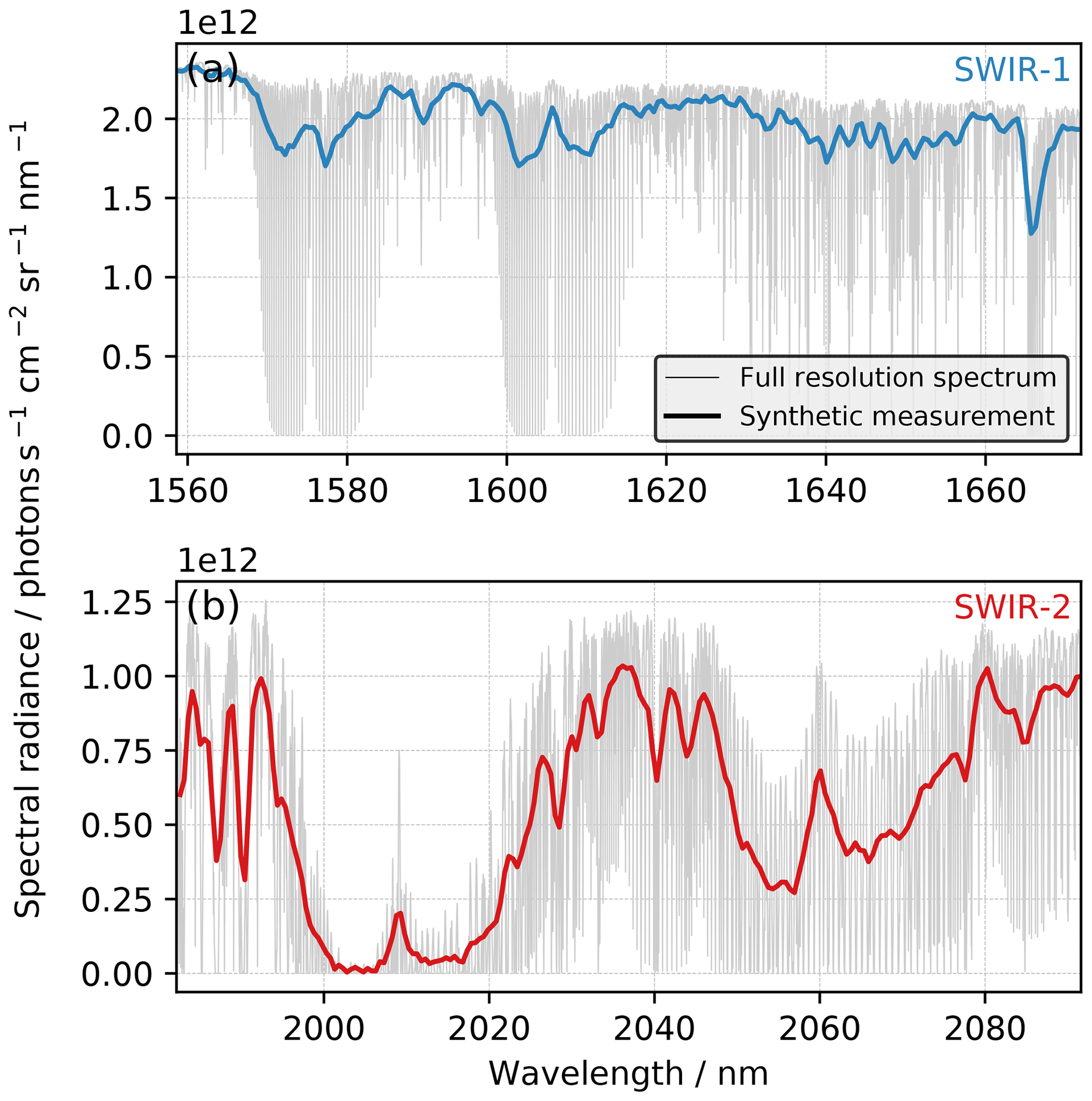
Figure 3Simulated synthetic measurements of spectral radiances for the two spectral setups near 1600 nm (SWIR-1) (a) and 2000 nm (SWIR-2) (b) for our reference scene with surface albedo 0.1 and an SZA of 70∘. Thin grey lines show corresponding spectral radiances at 0.003 nm spectral resolution.
The preliminary optical design assumes a circular aperture (15 cm in diameter) and is based on a three-mirror anastigmat (TMA) telescope, combined with an Offner-type spectrometer, as shown in Fig. 2. The optic system relies on metal-based mirrors and is designed as an athermal configuration for a wide temperature range onboard the satellite. The three mirrors of the TMA are standard aspheres aligned on a single optical axis. The efficiency of the optical bench (throughput), including transmittance and grating efficiency, is estimated to 0.48, and the f number (fnum), equal to the ratio of focal length to aperture diameter, amounts to 2.4. The dispersed electromagnetic radiation is focused onto a two-dimensional array detector that captures the spatial across-track dimension and the spectral dimension of the incoming radiation. A detector with a pixel area of 900 µm2 and a quantum efficiency of 0.8 is assumed for this study. The quantum efficiency depends on the wavelength but is for now assumed constant for both spectral windows. These values are in line with typical values for a state-of-the-art detector.
In order to reach a sufficient SNR, the proposed spatial resolution only allows for a relatively coarse spectral resolution. Wilzewski et al. (2020) used spectrally degraded GOSAT soundings to demonstrate the capability of retrieving XCO2 from a single spectral window at such a coarse spectral resolution using a spectral setup (in terms of spectral range, resolution and oversampling ratio) compact enough to fit onto 256 detector pixels. They evaluate two alternative spectral setups covering the spectral ranges 1559–1672 nm (hereafter also referred to as SWIR-1) and 1982–2092 nm (hereafter also referred to as SWIR-2) with a spectral resolution (full-width half-maximum – FWHM – of the instrument spectral response function) of 1.37 and 1.29 nm, respectively, and an oversampling ratio of 3. The resolving power of the SWIR-1 and SWIR-2 setups amounts to approximately 1200 and 1600, respectively. For optics design reasons, we use a spectral oversampling ratio of 2.5 in this study, resulting in a spectral sampling distance of 0.55 and 0.52 nm for SWIR-1 and SWIR-2, respectively. Simulated synthetic measurements of spectral radiances for the two prospective spectral setups are shown in Fig. 3, assuming a Gaussian instrument response function with an FWHM of 1.37 and 1.29 nm, respectively, as proposed by Wilzewski et al. (2020). The SWIR-1 window (Fig. 3a) exhibits two weak CO2 absorption bands around 1568–1585 nm and 1598–1615 nm and has the advantage of a stronger top-of-atmosphere (TOA) signal due to higher solar irradiance and surface albedo at these wavelengths. It also allows for the simultaneous retrieval of CH4 using the CH4 absorption band near 1666 nm. The SWIR-2 window, on the other hand, exhibits two stronger CO2 absorption bands around 1995–2035 and 2045–2080 nm and has higher sensitivity to atmospheric aerosol that can potentially be exploited during the XCO2 retrieval (Wilzewski et al., 2020). Wilzewski et al. (2020) showed similar performance for SWIR-1 and SWIR-2 but suspect SWIR-2 to be the favorable spectral setup given the stronger CO2 absorption bands, the ability to account for particle scattering and the lower radiance SNR required to reach sufficiently small XCO2 noise errors. In this paper, we further investigate the performance of the two spectral setups in order to finally conclude which is the more suitable one given the preliminary instrument design and realistic instrument SNR assumed here.
Table 1Mission and instrument design parameters of the proposed spaceborne CO2 monitoring instrument concept.
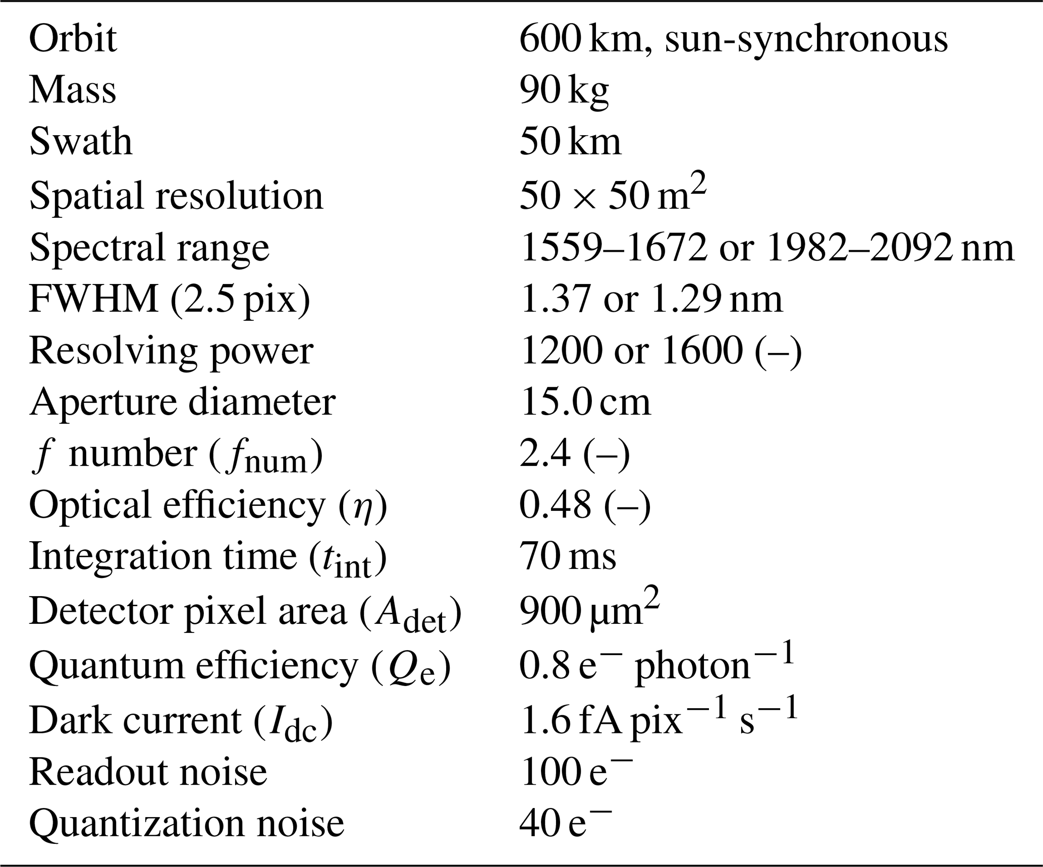
The instrument is designed to have a radiance SNR of 100 at the continuum for a reference scene with a Lambertian surface albedo of 0.1 and solar zenith angle (SZA) of 70∘. Given the altitude of 600 km and the corresponding orbital velocity of 7562 m s−1, the instrument traverses along one 50 m ground pixel in 7.2 ms. The number of photons collected over the course of 7.2 ms is, however, not enough to reach an SNR of 100. To increase the SNR, we suggest increasing the integration time to 70 ms. This would normally lead to elongated ground pixels (approx. 50×500 m2), but by using forward motion compensation (FMC), the instrument can be periodically altered in the along-track direction such that each ground pixel is sampled for a time period longer than the actual satellite overpass time (see, e.g., Sandau, 2010; Abdollahi et al., 2014). FMC has the evident drawback that the coverage along the satellite track is discontinuous, since no data are sampled when the instrument returns to the starting forward position. A second disadvantage is the geometrical distortion of the ground pixels that increases with the maximum off-nadir angle. The baseline design assumes 1000 measurements to be made in the along-track dimension for each FMC repetition, leading to off-nadir angles up to approximately 20∘. Further assuming 1000 detector pixels in the spatial dimension would consequently result in observed tiles on the order of 50×50 km2.
Table 1 summarizes the preliminary mission concept and instrument design parameters assumed for this study. It should be clear that this is a preliminary baseline design used to demonstrate the CO2 monitoring abilities and added value of the proposed instrument concept. Alternative instrument designs will be further investigated, and the exact instrument design will most likely be subject to change before the instrument is realized. The continuum SNR for our reference scene should nevertheless remain at roughly 100, ensuring a similar performance as presented in this paper.
To assess the performance of the proposed instrument concept with respect to retrieving XCO2 and resolving localized CO2 emissions, the expected instrument noise levels that accompany the measurements have to be quantified. To this end a numerical instrument noise model that calculates the instrument's SNR is developed, following a similar approach as, e.g., Bovensmann et al. (2010) and Butz et al. (2015). The SNR is given by
where S is the signal, i.e., the number of photons emerging from a 50×50 m2 ground pixel that generate a charge in the detector, and σtot is the corresponding instrument noise. The signal S is calculated as
where Lλ is the simulated reflected solar spectral radiance at the telescope, Adet the detector pixel area, fnum the instrument's f number, η the efficiency of the optical bench, Qe the detector's quantum efficiency, Δλ the wavelength range covered by a single detector pixel and tint the integration time between the detector pixel readouts. Following the thin lens equation (for large distances between a lens and an object) and the magnification formula, the term can also be expressed as Aap⋅Ω, where Aap is the area of the aperture (=πr2 with r=7.5 cm) and Ω the instrument's solid angle, i.e., the squared ratio of the ground sampling distance (50 m) over the orbit altitude (600 km). Apart from Lλ that is calculated for each scene using a forward radiative transfer model, all quantities in Eq. (2) and their corresponding values were introduced in Sect. 2.
The total noise σtot in Eq. (1) accounts for the noise contribution from five separate instrument noise sources:
where is the signal shot noise, σbg is the noise due to thermal background radiation incident on the detector, σdc is the noise due to dark current in the detector, σro is the noise upon detector readout and σqz the quantization noise that arises when the analog signal is digitized. The thermal background signal per detector pixel is approximated as
where EBB is the thermal black-body irradiance incident on the detector. EBB is determined by integrating the black-body spectral radiance Lλ,BB(Tbg) emitted by the background over the detector's cutoff wavelengths λ1 and λ2 and hemispheric opening angle,
For this study, detector cutoff wavelengths of 900 and 2500 nm are assumed, and the background temperature Tbg is estimated to 200 K. The thermal background noise is then calculated as . Similarly, the dark current noise is given by , where is the per-pixel detector signal due to dark current. While electrons C−1 is constant, the dark current Idc strongly depends on the detector's operating temperature and is estimated to 1.6 fA pix−1 s−1 (assuming 150 K detector temperature), yielding a dark current signal of approximately 10 000 electrons (e−) per detector pixel and second. Finally, the readout noise (σro) and quantization noise (σqz) are estimated to 100 and 40 e−, respectively. These noise levels are preliminary estimates used to test and evaluate the instrument concept but are comparable to those of state-of-the-art detectors for space applications.
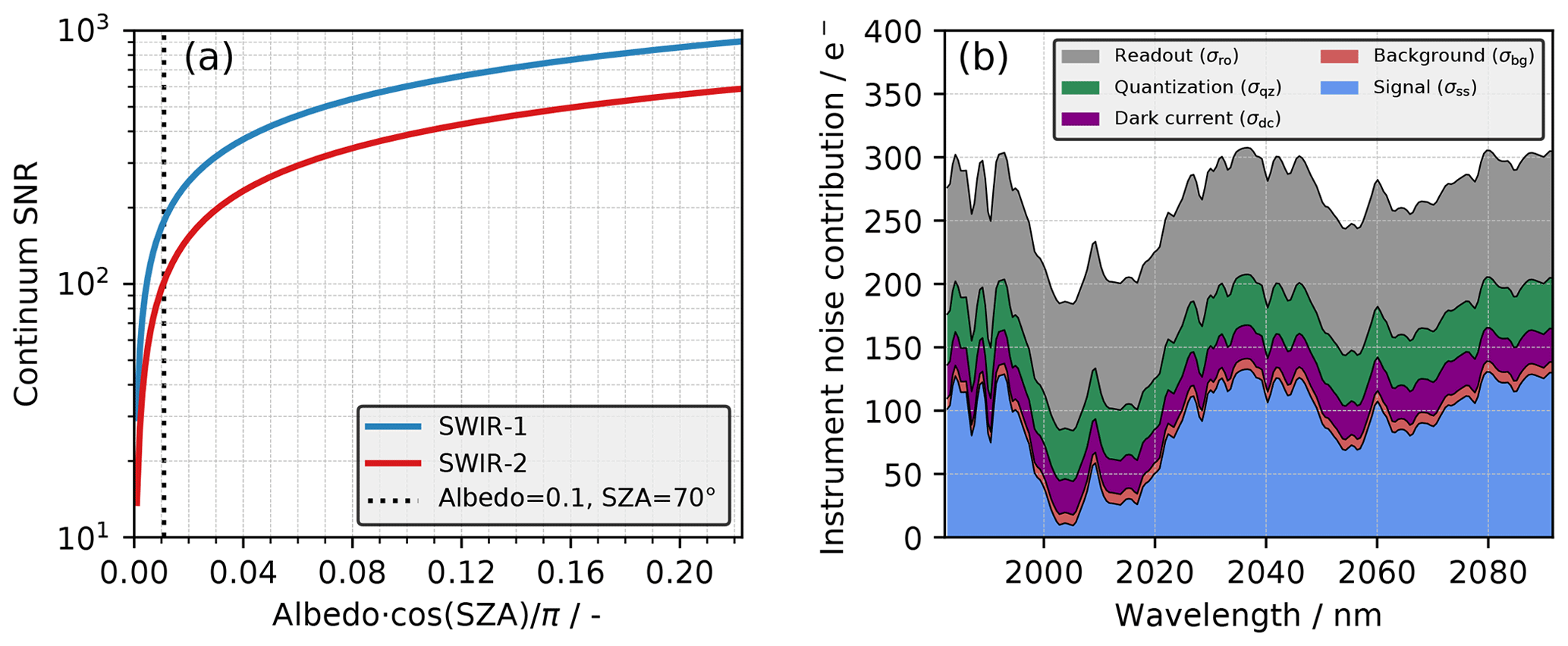
Figure 4(a) Continuum SNR as a function of scene brightness () for the SWIR-1 and SWIR-2 spectral setups, with the dotted line indicating the brightness of our reference scene. The highest scene brightness (approx. 0.22) represents a bright scene with an albedo of 0.7 and an SZA of 0∘. (b) Instrument noise contributions for a simulated SWIR-2 spectrum.
Figure 4a shows the continuum SNR (calculated with Eqs. 1–5) as a function of the scene brightness for the two prospective spectral setups SWIR-1 and SWIR-2. The scene brightness describes the conversion from incident solar irradiance to reflected solar radiance and is calculated as the product of the surface albedo and the cosine of the SZA divided by π, hence assuming a Lambertian surface. For the reference scene (albedo 0.1, SZA 70∘), the continuum SNR is approximately 180 and 100 for SWIR-1 and SWIR-2, respectively. The consistently higher SNR for SWIR-1 compared to SWIR-2 is mainly the result of higher solar radiance (see Fig. 3) and generally higher surface albedo (see, e.g., Fig. 7 in Butz et al., 2009) in SWIR-1. Looking at the individual contributions from the different instrument noise sources in Fig. 4b, it is clear that the readout noise and signal shot noise are the major contributors, whereas the noise arising from quantization errors, dark current and thermal background radiation has a small or even negligible contribution in comparison. The signal shot noise is, however, smaller than the dark current, readout noise and quantization noise inside the CO2 absorption bands, in which the signal, and hence the signal shot noise, decreases. Note that all noise terms except for the signal shot noise, σss, are constant.
In this section we conduct a first performance evaluation of the proposed instrument concept by assessing the XCO2 retrieval errors expected on a global scale. Such errors arise due to instrument noise and because of inadequate knowledge about the light path through the atmosphere due to scattering aerosol and cirrus particles. For this purpose we use a global trial ensemble with a large collection of geophysical scenarios with varying atmospheric gas concentrations, meteorological conditions, surface albedo, SZA, and aerosol and cirrus compositions that can be expected to be observed by a polar-orbiting instrument. The same methodology and dataset have been used in several previous studies to assess the greenhouse gas retrieval performance of different satellite instruments (Butz et al., 2009, 2010, 2012, 2015).
The global trial ensemble contains geophysical data representative for the months of January, April, July and October. Atmospheric gas concentrations stem from the CarbonTracker model (CO2 for the year 2010; Peters et al., 2007), the Tracer Model 4 (CH4 for the year 2006; Meirink et al., 2006) and the ECHAM5-HAM model (H2O; Stier et al., 2005). Surface albedo data representative for the SWIR-1 and SWIR-2 windows stem from the MODIS (Moderate Resolution Imaging Spectroradiometer) MCD43A4 product (Schaaf et al., 2002). Aerosol optical properties are calculated (assuming Mie scattering) for an aerosol size distribution superimposed from seven lognormal size distributions and five chemical types at 19 vertical layers, as provided by the ECHAM5-HAM model (Stier et al., 2005). Cirrus optical properties are calculated for randomly oriented hexagonal columns and plates following the ray-tracing model of Hess and Wiegner (1994) and Hess et al. (1998). In total the global trial ensemble consists of approximately 10 000 scenes with XCO2 ranging from 340 to 400 ppm with an average of 382 ppm, albedo ranging from 0 to 0.7 with an average of 0.13 (SWIR-2 window), aerosol optical thickness (AOT) ranging from 0 to 1.0 with an average of 0.05 (SWIR-2 window) and cirrus optical thickness (COT) ranging from 0 to 0.8 with an average of 0.13 (SWIR-2 window). Thus, the global trial ensemble contains challenging scenes with scattering loads that would be filtered out by current satellite retrievals, such as those applied to OCO-2 and GOSAT data, which typically screen scenes with scattering optical thickness greater than 0.3 (at the O2 A band around 760 nm). All data in the global trial ensemble are re-gridded to a spatial resolution of approximately 2.8∘ × 2.8∘. This is, of course, much coarser than the envisaged 50×50 m2, but for investigating the propagation of instrument noise into the target quantity XCO2 on a global scale, this dataset serves its purpose. See previous studies (e.g., Butz et al., 2009, 2010) for further details on the content of the global trial ensemble.
The geophysical data for each scene are fed to the radiative transfer software RemoTeC (Butz et al., 2011; Schepers et al., 2014) in order to simulate corresponding synthetic measurements. The measurement noise is calculated by propagating the instrument's SNR (Sect. 3) into a statistical error estimate according to the rules of Gaussian error propagation (Rodgers, 2000). Simulations are conducted globally for the 16th day of each of the four months January, April, July and October, hence covering SZA conditions ranging from 0 to 86∘.
By retrieving XCO2 from the simulated synthetic spectra, the range of XCO2 retrieval errors that can be expected with the proposed instrument concept can be estimated, as can the ability to account for atmospheric aerosol. The RemoTeC retrieval algorithm (e.g., Butz et al., 2011) is based on a Philipps–Tikhonov regularization scheme (Phillips, 1962; Tikhonov, 1963) that uses the first-order difference operator as a side constraint to retrieve the CO2 partial column profiles, from which XCO2 can be determined. Additional retrieval parameters are the total column concentrations of H2O and CH4 (only for SWIR-1), surface albedo (as a second-order polynomial), spectral shift, solar shift, and possibly information on scattering aerosol. Here we assume knowledge about the air mass (needed to calculate XCO2), but in reality meteorological and topography data would be required to estimate the air mass.
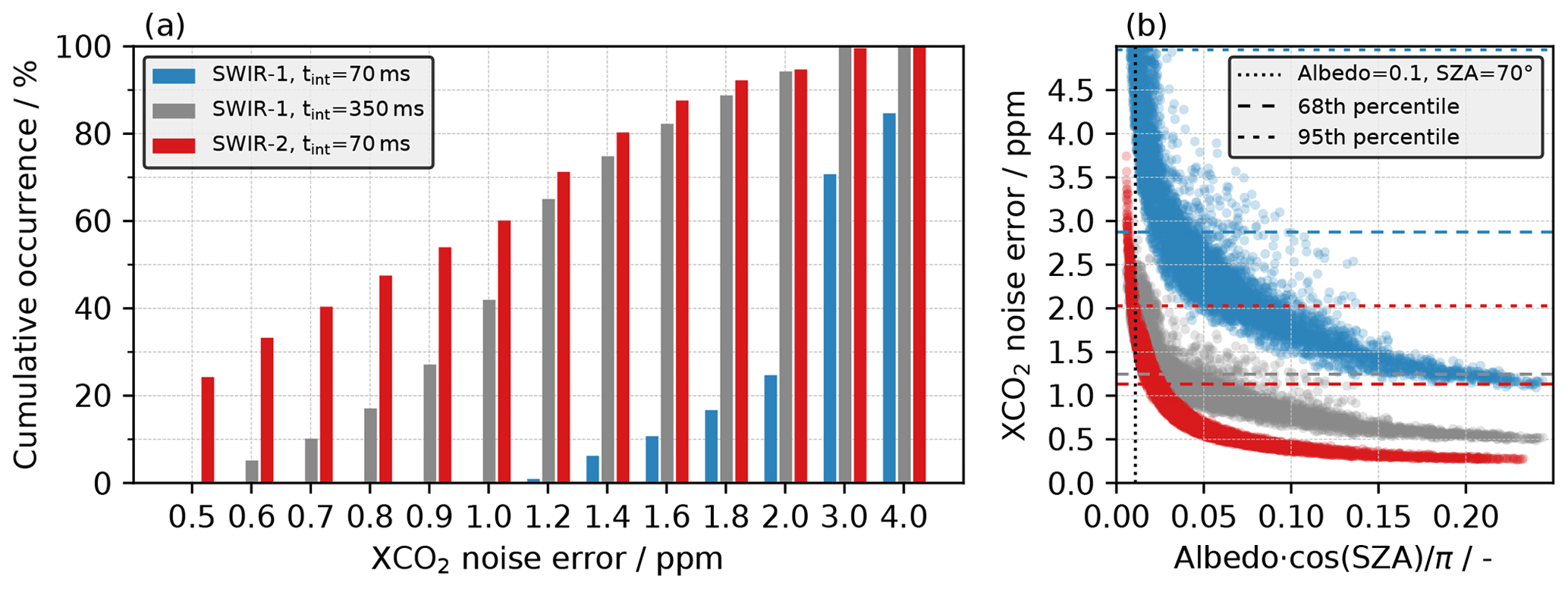
Figure 5(a) Cumulative distribution of the estimated XCO2 noise errors arising from instrument noise for all scenes in the global ensemble. (b) XCO2 noise errors as a function of surface brightness, with the dotted line indicating our reference scene and the dashed lines indicating the 68th and 95th percentiles of the XCO2 noise errors for the different spectral setups. Note that the red and grey lines for the 95th percentile overlap at 2.03 ppm. Marker colors in (b) correspond to those in (a). Both panels show the results for the SWIR-1 (blue) and SWIR-2 (red) setups as well as for an alternative SWIR-1 (grey) setup for comparison (see the text for details).
4.1 Instrument-noise-induced XCO2 errors
In a first step, we assess XCO2 retrieval errors that are induced by instrument noise. To this end, for now, we neglect scattering by aerosol and cirrus. These so-called non-scattering simulations assume no scattering particles to be present in the atmosphere and simply compute the transmittance along the geometric light path (Rayleigh scattering is included).
Figure 5a shows the cumulative distribution of the random XCO2 noise error, i.e., the instrument noise propagated into XCO2 uncertainties via Gaussian error propagation. Furthermore, Fig. 5b shows the XCO2 noise error for each simulated scene as a function of the corresponding scene brightness. The noise errors are significantly smaller for the SWIR-2 setup (red) when using the proposed integration time tint of 70 ms. The red dashed lines in Fig. 5b show that on average 68 % and 95 % (1σ and 2σ, respectively) of the retrievals have noise errors of less than approximately 1.1 and 2.0 ppm, respectively. For the SWIR-1 setup (blue), the corresponding numbers are 2.9 and 5.0 ppm. For the SWIR-2 setup, only retrievals over scenes that are darker than our reference scene (albedo 0.1, SZA 70∘) are expected to have instrument-noise-induced errors larger than approximately 2 ppm. For comparison and as a reference, we also investigate how much the integration time has to be increased for the SWIR-1 setup in order to reach an SNR sufficient to yield XCO2 noise errors comparable to those obtained with the SWIR-2 setup. We find that with the preliminary instrument design assumed here, the integration time has to be increased to at least 350 ms (i.e., by a factor of 5) for SWIR-1 (grey) in order to reach a similar performance.
Despite the advantage of being able to retrieve XCH4 alongside XCO2 using the SWIR-1 setup, the much longer integration time required to reach sufficiently low CO2 noise errors is not feasible for the purpose of the proposed instrument concept. Hence, we conclude that the SWIR-2 setup is superior for the passive satellite-based CO2 monitoring instrument proposed in this paper. Consequently, the remainder of this paper is limited to the SWIR-2 setup, covering the spectral range 1982–2092 nm with a spectral resolution (FWHM) of 1.29 nm, resolving power around 1600 and a spectral sampling distance of 0.52 nm.
4.2 Aerosol-induced XCO2 errors
Atmospheric aerosol and cirrus particles modify the light path of the reflected solar radiation to a certain degree, depending on the particle abundance, optical properties, height and surface albedo. Consequently, this can cause large errors in the retrieved XCO2 if the effect of CO2 absorption and particle scattering on the measured reflected solar radiation cannot be adequately separated during the retrieval process. In this section the ability to account for atmospheric aerosol and cirrus during the retrieval is investigated by including scattering by atmospheric particles in the simulation of the synthetic measurements and in the corresponding XCO2 retrievals. This is done by using a more complex forward model and representation of the aerosol and cirrus particles when simulating the spectra, as well as a comparatively simple representation and forward model for the corresponding retrievals. More precisely, the full physical representation of the vertical profiles of hexagonal cirrus particles and spherical aerosol particles of the five chemical types characterized by the seven lognormal size distributions with known microphysical properties for each aerosol and cirrus particle type is used when simulating the synthetic measurement for each scene in the global trial ensemble. In contrast, only three aerosol parameters are fitted during the corresponding retrieval: the total column number density, the size parameter of a single-mode power-law size distribution and the center height of a Gaussian height distribution. Such differences in the aerosol and cirrus representation lead to forward model errors that, alongside the instrument-noise-induced errors, propagate into the retrieved quantity XCO2. Previous studies have shown that this approach gives a good approximation of how well a satellite sensor can account for scattering by atmospheric aerosol while retrieving target gas concentrations (e.g., Butz et al., 2009, 2010).
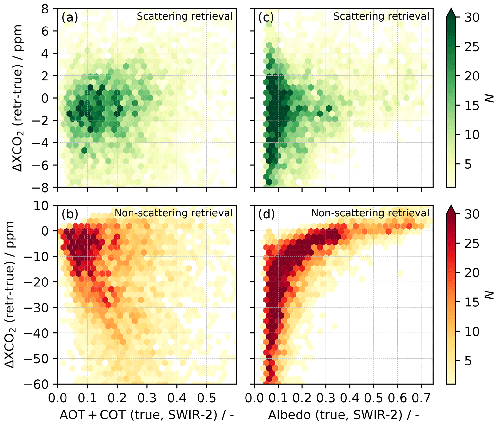
Figure 6(a, b) XCO2 retrieval errors as a function of the total particulate optical thickness AOT+COT for scattering (a) and non-scattering (b) RemoTeC retrievals. (c, d) XCO2 retrieval errors as a function of SWIR-2 surface albedo for scattering (c) and non-scattering (d) RemoTeC retrievals. N denotes the number of retrievals. Note the different ranges of the y axes in the upper and lower panels.
Figure 6a shows the difference between the XCO2 retrieved (“retr”) from the synthetic measurements and the corresponding “true” XCO2 used as input to simulate these synthetic measurements. This deviation from the truth contains information on both random instrument noise error (Sect. 4.1) and systematic errors arising from insufficient modeling of the aerosol and cirrus properties. For comparison, Fig. 6b shows the corresponding results achieved when using a non-scattering retrieval, i.e., when the scattering by atmospheric aerosol and cirrus, now present in the atmosphere and the simulated synthetic spectra, is neglected (similar to Sect. 4.1). The retrieval errors are strongly reduced when the RemoTeC retrieval algorithm accounts for the scattering by atmospheric aerosol. When scattering is considered, half of the XCO2 retrievals deviate from the true abundance by less than 2.5 ppm, while two-thirds of the retrievals deviate by less than 4 ppm (approx. 1 %), with no clear error correlation with the optical thickness of the scattering particles. For the non-scattering retrieval, the corresponding numbers are 16 and 28 ppm, with a mean bias of −25 ppm that increases with optical thickness, exposing the necessity of accounting for atmospheric aerosol and cirrus when retrieving the XCO2.
Scattering particles can modify the light path and hence the XCO2 retrieval in primarily two ways. Firstly, an elevated layer of aerosol or cirrus will scatter parts of the incoming solar radiation towards the observing sensor at a higher altitude compared to the Earth's surface, leading to a reduced light path. Secondly, aerosol and cirrus will extend the light path to some degree as a result of multiple scattering between scattering particles and the surface. Such modifications of the light path will be understood as CO2 concentrations in the atmosphere that are either too low (overall reduced light path) or too high (overall extended light path) if scattering cannot be accounted for in the retrieval. Which effect dominates is primarily driven by the surface albedo. This is visualized in Fig. 6d that shows the difference between retrieved and true XCO2 as a function of the surface albedo when scattering by aerosol and cirrus is neglected in the retrieval. Over darker surfaces for which the effect of multiple scattering between aerosol and the surface is limited, aerosol and cirrus particles scattering the incoming solar radiation towards the sensor higher up in the atmosphere become the dominating effect, leading to a reduced light path and underestimation of the XCO2. Over brighter surfaces for which the effect of multiple scattering becomes dominant, the non-scattering retrieval is more likely to overestimate the CO2 abundance because the loss of radiation due to an extended light path, resulting from the multiple scattering, is assumed to be caused by more absorbing CO2 molecules in the atmosphere. Figure 6c shows the difference between retrieved and true XCO2 as a function of the surface albedo when scattering by aerosol and cirrus is accounted for when retrieving XCO2 from the synthetic measurements of the proposed satellite concept. It is clear that when aerosol properties are retrieved alongside the CO2 abundance, the curve-shaped relationship between the XCO2 error and surface albedo vanishes with no clear error correlation other than XCO2 errors increasing with decreasing albedo (and thus SNR). Note that errors arising from the Lambertian albedo assumption (BRDF – bidirectional reflectance distribution function – effects) are neglected in the scattering simulations.
Although layers of aerosol and cirrus can be partly accounted for in the retrieval, scenes with thicker clouds and aerosol layers will have to be identified and filtered out in the data processing chain. Such a cloud filter could exploit the different optical depths of the two CO2 bands in the SWIR-2 window by retrieving XCO2 from the two CO2 bands independently (assuming a non-scattering atmosphere) and filtering for discrepancies.
While the previous section assessed XCO2 errors for the range of geophysical conditions expected to be encountered on a global scale, this section evaluates the CO2 monitoring capabilities at an urban scale using high-resolution CO2 concentration and surface albedo data. Similar to Sect. 4, the high-resolution data are used to simulate synthetic measurements, from which synthetic XCO2 abundances can be retrieved in order to make a first assessment of the CO2 monitoring ability of the proposed instrument concept in terms of resolving CO2 emission plumes.
5.1 Datasets
5.1.1 CO2 concentration field from the Hestia dataset
To compute a high-resolution three-dimensional field of CO2 concentrations to be used as input for the radiative transfer simulations, annual estimates of fossil fuel CO2 emissions for the city of Indianapolis in the year 2015 are used. These data are generated by the Hestia Project (Gurney et al., 2012, 2019) for which the fossil fuel CO2 emissions are quantified in urban areas down to the scale of individual buildings and streets using a bottom-up approach. The results for the city of Indianapolis are gridded and archived at a spatial resolution of 200×200 m2. For this study, however, the Hestia Project dataset was gridded to 50×50 m2 via request to the Hestia research team in order to match the envisaged spatial resolution of the proposed instrument concept. The fossil fuel CO2 emission rates for Indianapolis at 50×50 m2 resolution can be seen in Fig. 7a. CO2 emissions from different sources and sectors like road traffic and point sources (single yellow pixels) can be seen. There is also an apparent emission gradient, with stronger emissions in the city center and weaker emissions towards the suburbs. Hence, the Hestia CO2 emission data for Indianapolis provide a realistic emission scenario for evaluating the CO2 monitoring capabilities of the proposed instrument concept. Moreover, the area of the Hestia domain (approx. 34×33 km2) is comparable to what the prospective tile size of each observation target area could be.
The Hestia CO2 emission data are used as input to a Gaussian dispersion model in order to compute a three-dimensional CO2 concentration field. For a given CO2 emission rate Q (g s−1), the CO2 concentration C (g m−3) at a given position () downwind of the emitter is calculated as
where u is the horizontal wind speed in the x direction (along-wind), h is the height of the emitting source (in meters above ground level), and σy and σz are the standard deviations of the concentration distribution (in meters) in the horizontal across-wind and vertical dimension, respectively; σy and σz, and hence the spread of the emission plume, depend on the atmospheric instability, i.e., the degree of atmospheric turbulence and the downwind distance x from the emitting source. Here, we calculate σy and σz assuming the Pasquill–Gifford stability class C (slightly unstable atmosphere). Furthermore, a constant wind speed u=3 m s−2 and an emitting source height h=75 m (for all sources) are assumed. This model setup is comparable to similar studies (e.g., Bovensmann et al., 2010; Dennison et al., 2013).
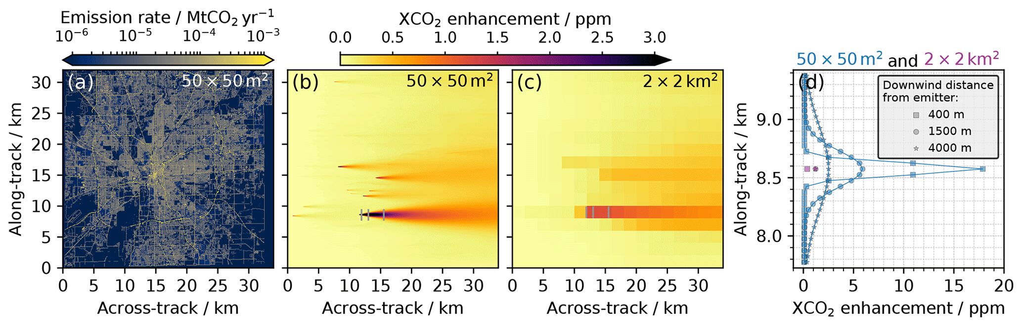
Figure 7(a) Hestia fossil fuel CO2 emission data for Indianapolis in 2015 at 50×50 m2 spatial resolution. (b) Corresponding field of vertically integrated XCO2 enhancements at 50×50 m2 spatial resolution with respect to a constant background, computed using the Hestia CO2 emission data and a Gaussian dispersion model. Panel (c) is the same as (b), but at 2×2 km2 spatial resolution. (d) Per-pixel XCO2 enhancements for three along-track excerpts centered at 400, 1500 and 4000 m downwind of the emitter at 50×50 m2 and 2×2 km2 spatial resolution. The respective positions of the along-track excerpts are indicated by the small grey lines in (b) and (c). The x and y dimensions of the Hestia Indianapolis domain are illustrated as hypothetical satellite across-track and along-track dimensions, respectively.
Downwind CO2 concentrations from each emitting source (pixel) in the Hestia dataset are calculated across an equidistant grid at 50 m resolution in all dimensions, and the contributions from all individual emitting sources (pixels) are subsequently combined to form a three-dimensional CO2 concentration field over Indianapolis. Figure 7b shows the resulting (vertically integrated) two-dimensional field of (noiseless) XCO2 enhancements at 50×50 m2 spatial resolution over a constant background with a surface pressure of 1013 hPa. While weaker diffuse sources like streets cannot be identified, the plumes from stronger point sources are clearly pronounced given the high spatial resolution that allows for a detailed mapping of the plumes. For comparison, Fig. 7c shows the corresponding XCO2 enhancements assuming a coarser spatial resolution of 2×2 km2. Although the stronger plumes can still be identified at the coarser resolution, the XCO2 enhancements are significantly lower and each plume is only sampled by a few pixels. Figure 7d further shows these XCO2 enhancements in more detail for three along-track excerpts centered at 400, 1500 and 4000 m downwind of the strongest emitter in Indianapolis, with an annual emission rate of 3.24 Mt CO2 yr−1 in 2015. The positions of the three along-track excerpts are indicated with grey lines in Fig. 7b and c. With a spatial resolution of 2×2 km2, the along-track plume excerpts are only sampled by one pixel each, with a maximum XCO2 enhancement of 1.2 ppm. With the envisaged 50×50 m2 spatial resolution, however, the plume is sampled by 7, 15 and 29 pixels in the along-track dimension 400, 1500 and 4000 m downwind of the emitter, respectively, with maximum XCO2 enhancements reaching approximately 18, 6 and 3 ppm, respectively. This clearly demonstrates the benefit of an instrument with a high spatial resolution when resolving CO2 emission plumes from space.
5.1.2 Surface albedo data from Sentinel-2
To accurately simulate the instrument SNR and hence the measurement noise, it is important to know how large a fraction of the solar radiation incident on the Earth's surface is reflected back towards space. To get realistic estimates of the surface albedo within the Hestia Indianapolis domain, data from the European Sentinel-2 satellites are used. The multispectral instrument aboard Sentinel-2 measures the TOA radiance in 13 spectral bands with a spatial resolution ranging from 10×10 m2 to 60×60 m2. For this study, we use the Sentinel-2 L1C radiances measured in spectral band 12 (centered at approx. 2200 nm) at a spatial resolution of 20×20 m2. The software Sen2Cor (ESA, 2018) is employed to compute the corresponding L2 surface reflectances from the L1C TOA radiances through a so-called atmospheric correction.
Surface reflectance data for the month of July 2018 are computed and re-gridded (using nearest neighbor) to the envisaged spatial resolution of 50×50 m2. The surface reflectance for Sentinel-2 pixels classified as vegetation is scaled by a factor of 0.82 in order to account for the generally lower reflectance by vegetation in the SWIR-2 window compared to Sentinel-2's band 12. The scaling factor has been derived using spectral reflectance data from the ECOSTRESS spectral library (Baldridge et al., 2009; Meerdink et al., 2019). Figure 8b shows the gridded surface reflectance data for Indianapolis together with a corresponding red–green–blue (RGB) composite (Fig. 8a) using Sentinel-2 data from the bands centered at red, green and blue wavelengths as a reference. The scaled and gridded Sentinel-2 surface reflectance data are taken as representative for a constant Lambertian surface albedo within the entire SWIR-2 window. Figure S1 in the Supplement shows spectral reflectances in the SWIR spectral region for various urban materials using data from the Spectral Library of impervious Urban Materials (SLUM; Kotthaus et al., 2014). The small spectral variations within the SWIR-2 spectral window used in this study indicate that the true spectral signatures of the surface albedo could be fitted with sufficient precision using the second-order polynomial during the retrieval, and hence the assumption of a constant albedo is reasonable for this study.
The average surface reflectance within the Hestia domain is 0.13. Despite annual variability in surface reflectance, mainly due to changes in vegetation and/or crops, this is a value representative throughout most of the year. For comparison, average surface reflectances from the same source for January (snow-free days), April and October 2018 amount to 0.11, 0.17 and 0.11, respectively.
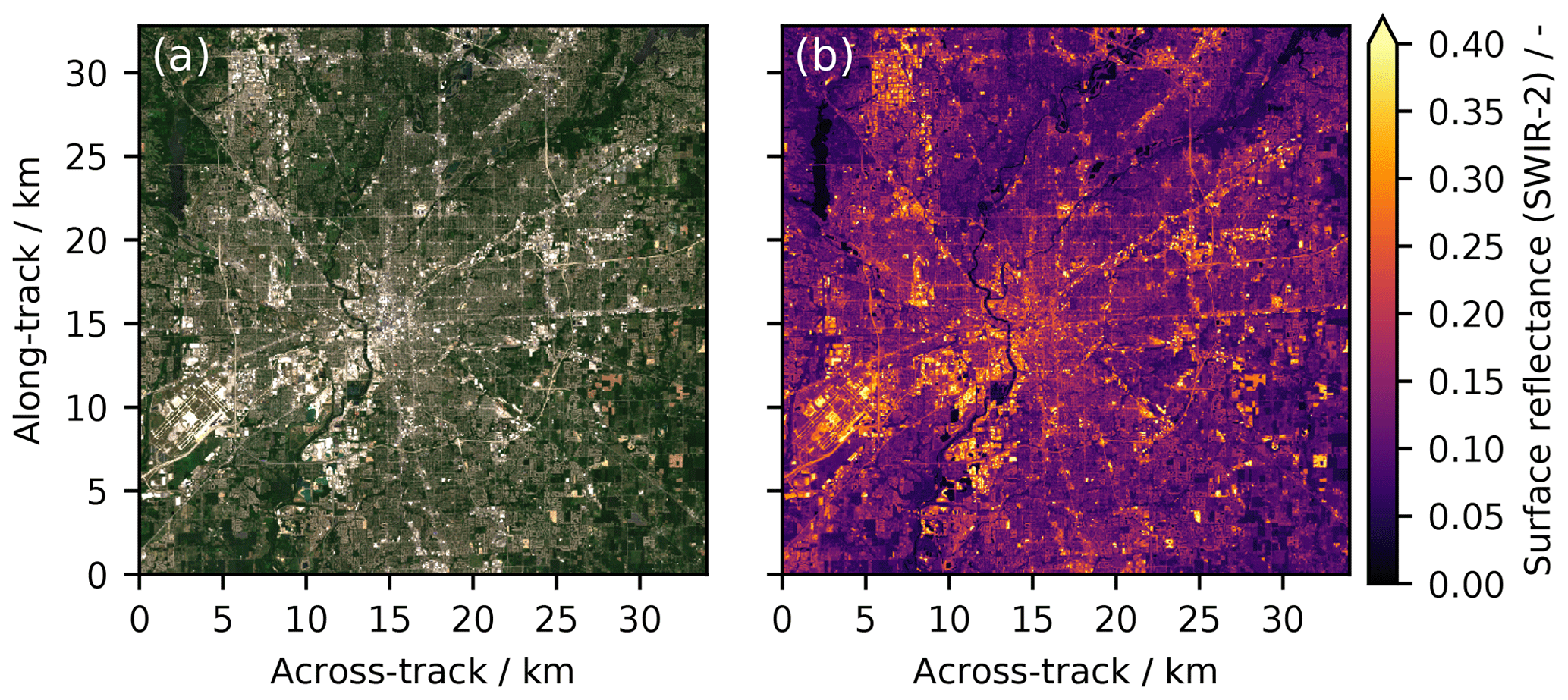
Figure 8(a) Sentinel-2 true-color RGB image of Indianapolis (Hestia domain) at 50×50 m2 spatial resolution derived from Sentinel-2 measurements in July 2018. (b) Corresponding surface reflectance data using data from Sentinel-2's spectral band 12 centered at approximately 2200 nm, scaled to the SWIR-2 spectral window. Again, the x and y dimensions of the Hestia Indianapolis domain are illustrated as hypothetical satellite across-track and along-track dimensions, respectively.
5.1.3 Background data from CarbonTracker
Background data, including vertical profiles of CO2, H2O, temperature and pressure, are taken for 15 July 2016 from the CarbonTracker CT2017 dataset (Peters et al., 2007, with updates documented at http://carbontracker.noaa.gov, last access: 18 March 2019). The CarbonTracker CT2017 data over Indianapolis are provided at a spatial resolution of 1∘ × 1∘, meaning that the entire Hestia Indianapolis domain is covered by one single CarbonTracker pixel, leading to a constant background data field.
5.2 Simulated CO2 plume observations
As in Sect. 4, the above sets of input data are used to simulate synthetic measurements (spectral radiances) and the corresponding instrument noise of the proposed instrument concept using the forward model and the instrument noise model (Sect. 3). The SZA is calculated for the given coordinates in the Hestia domain assuming the sun-synchronous orbit described in Sect. 2 and an observation date of 15 July 2018, which translates to an SZA of about 18∘. Corresponding XCO2 abundances are then retrieved from the simulated spectral radiances such that the ability to observe the CO2 emission plumes from the Hestia Indianapolis data can be evaluated. In this first assessment we focus solely on the instrument performance in terms of its CO2 plume quantification capabilities, and hence we perform the high-resolution simulations with the expected instrument-noise-induced errors only, i.e., by assuming a non-scattering atmosphere.
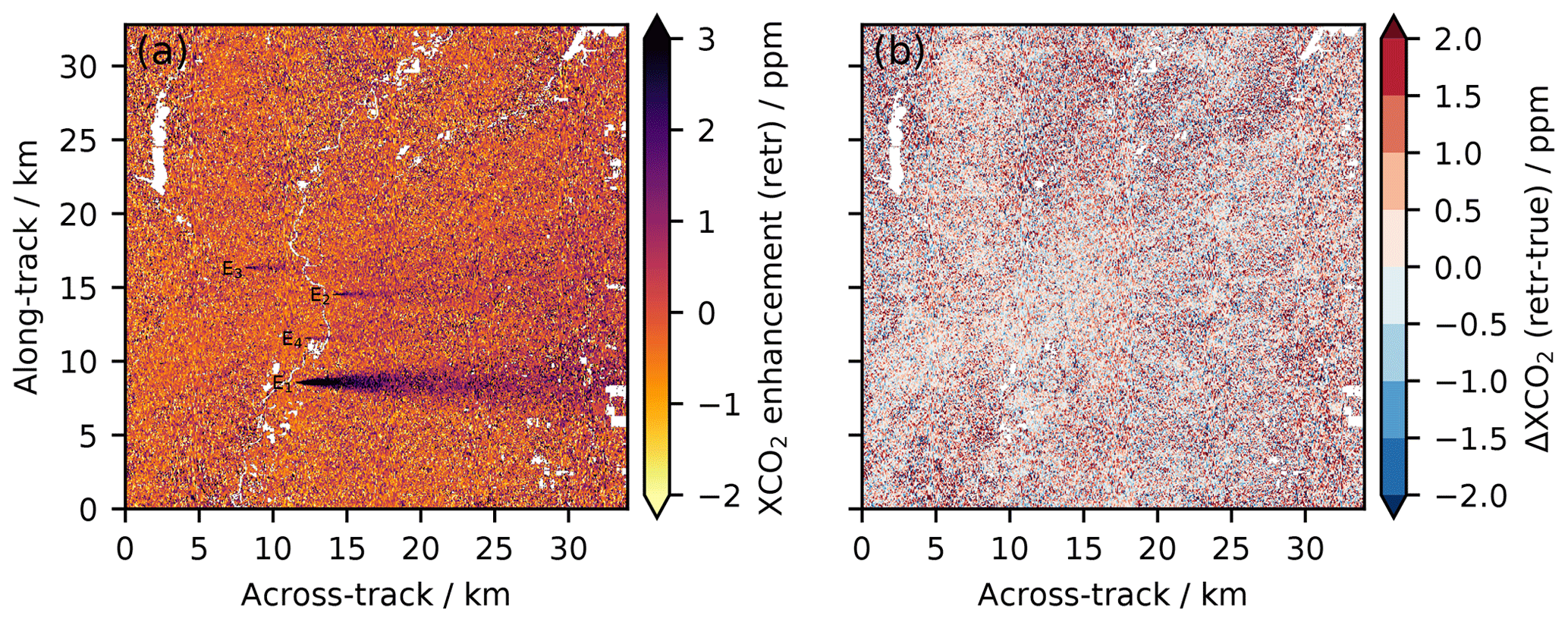
Figure 9(a) XCO2 enhancements with respect to the background retrieved from the simulated synthetic measurements over the Hestia Indianapolis domain under non-scattering conditions. Locations of the four strongest point sources are labeled with E1−4. (b) Corresponding deviations between retrieved (“retr”) and true XCO2. Dark scenes with albedo <0.05 have been filtered out due to unreliable XCO2 retrievals.
Figure 9a shows the retrieved field of XCO2 enhancements with respect to the retrieved background XCO2 over the Hestia domain. The CO2 plume from the strongest point source, E1, with an annual CO2 emission rate of Q1=3.24 Mt CO2 yr−1, is clearly resolved with local XCO2 enhancements well above 100 ppm close to the emitting source. Although they emit considerably less CO2, the plumes from the second- and third-strongest point sources, E2 and E3, with annual CO2 emission rates of Q2=0.55 Mt CO2 yr−1 and Q3=0.48 Mt CO2 yr−1, respectively, can be clearly separated from the background as well. The plume from the fourth-strongest point source, E4, with an annual CO2 emission rate of Q4=0.32 Mt CO2 yr−1, can also be observed but is partly obscured by filtered-out dark surface areas for which retrieval errors are too high. Plumes from weaker point sources (≲0.1 Mt CO2 yr−1) and other sources like streets and highways cannot be identified given the spatial resolution and instrument noise errors of the proposed instrument.
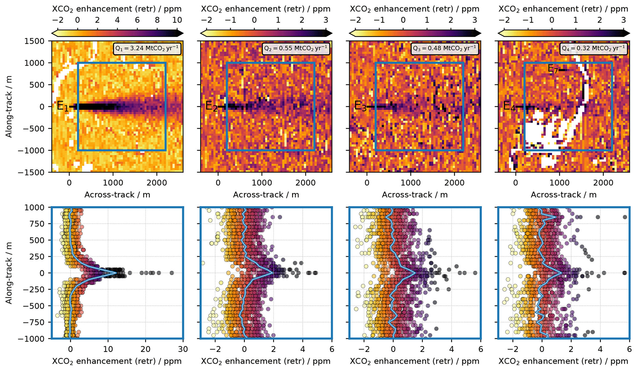
Figure 10Upper panels: retrieved two-dimensional fields of XCO2 enhancements in the vicinity of the four strongest CO2 emitters E1, E2, E3 and E4 within the Hestia Indianapolis dataset. Lower panels: corresponding per-pixel (circles) and average (solid lines) along-track XCO2 enhancements within the area 200 to 2200 m downwind and −1000 to 1000 across-wind of the respective emitters. The blue rectangles in the upper panels show the areas from which the corresponding per-pixel and average along-track XCO2 enhancements, depicted in the respective lower panels, are extracted and calculated. The color of the circles follows the color bars in the respective upper panels.
One concern with high-resolution CO2 remote sensing is the impact of albedo heterogeneity at an urban scale at such a high spatial resolution. For the non-scattering scenario simulated here, the albedo fitted by the retrieval algorithm matches the reference input albedo with an average (absolute) deviation of 0.14 %, and there is consequently no spatial variability in the accuracy of the albedo retrieval that in turn affects the XCO2 retrieval accuracy. There is, however, the evident effect that a higher albedo leads to a higher SNR and hence a generally lower noise error. This is evident from Fig. 9b, showing the difference between the retrieved and true XCO2, thus illustrating an instantaneous noise error field that would be expected for a single satellite overpass. Generally, the deviations from the true XCO2 are smaller over areas of brighter surfaces like concrete, whereas the deviations are larger over dark surfaces like forests (see also Fig. 8). The effect of albedo heterogeneity in combination with scattering particles is not addressed in this paper and will have to be analyzed in future studies.
Across the entire Hestia domain (but excluding dark scenes with albedo <0.05) 68 % and 95 % of the XCO2 retrievals deviate from the true XCO2 by less than 1.1 and 2.3 ppm, respectively. This is comparable to the noise error obtained for the global trial ensemble in Sect. 4.1 (1.1 and 2.0 ppm, respectively).
Figure 10 shows close-ups of the simulated XCO2 enhancement field (upper panels) in the vicinity of the four strongest emitters in the Hestia Indianapolis dataset (E1–E4 in Fig. 9a), along with the corresponding per-pixel and average along-track XCO2 enhancements (lower panels) for the range 200–2200 m downwind of the respective emitting sources. Enhancements from the 200 m closest to each emitting source are excluded as those scenes could likely be obscured by condensate in a real situation.
The plume of the strongest emitter E1 in Indianapolis with an annual emission rate of Q1=3.24 Mt CO2 yr−1 is clearly resolved. Within the area 200–2200 m downwind of the emitting source (blue square), maximum enhancements exceed 25 ppm, and in total, approximately 200 (60) pixels have enhancements above 4 ppm (8 ppm), representing enhancements of approximately 1 % (2 %) with respect to the background. The average along-track XCO2 enhancement 200–2200 m downwind of the emitting source (blue and white line) reaches 12 ppm. The plumes from the second- and third-strongest emitters, E2 and E3, which are approximately 6 times weaker than E1 with annual emission rates of Q2=0.55 and Q3=0.48 Mt CO2 yr−1, respectively, have considerably lower XCO2 enhancements but can nevertheless clearly be separated from the background with distinct increments in both per-pixel and average XCO2 enhancements within the area 200–2200 m downwind of the emitters (blue squares). While the background fields vary from approximately −1 to 1 ppm due to instrument noise, the per-pixel plume enhancements vary from approximately 0.5 to 3 ppm, with single enhancements exceeding 4 ppm close to the emitting source. The average along-track XCO2 enhancements 200–2200 m downwind of the emitting sources (blue and white lines) reach 1.9 and 1.5 ppm for E2 and E3, respectively. Despite being partly obscured by filtered-out dark surfaces (water), the plume from the fourth-strongest emitter E4, with an annual emission rate of Q4=0.32 Mt CO2 yr−1, can also be separated from the background both when looking at the two-dimensional field and the per-pixel enhancements within the area 200–2200 m downwind of the emitter. With maximum average XCO2 enhancements of at most approximately 1.3 ppm, the proposed instrument concept is, however, approaching the limit of what it could achieve in terms of CO2 plume observations under favorable conditions, i.e., when the effect of aerosol-induced errors is neglected and the SZA is relatively low. A second peak in the average along-track XCO2 enhancements is observed approximately 850 m above (north of) the fourth-strongest emitter E4. This enhancement stems from the CO2 plume from the seventh-strongest emitter in Indianapolis (labeled E7 in the top right panel of Fig. 10), with an annual emission rate of Q7=0.1 Mt CO2 yr−1. Quantifying the CO2 emission rate from such a weak source is, however, not realistic given the low sampling density (especially further downwind) in combination with the weak per-pixel enhancements.
To follow the progress on reducing anthropogenic CO2 emissions worldwide, independent monitoring systems are of key importance. In this paper, we present the concept of a compact spaceborne imaging spectrometer with a high spatial resolution of 50×50 m2 targeting the monitoring of localized CO2 emissions. We further demonstrate how the instrument concept could resolve CO2 emission plumes from localized point sources like medium-sized power plants, thus having the potential to contribute to the independent large-scale verification of reported CO2 emissions at the facility level.
Through radiative transfer simulations using a global trial ensemble, a preliminary yet realistic instrument design and an instrument noise model, we show that the expected instrument-noise-induced XCO2 errors are smaller than 1.1 and 2.0 ppm for 68 % and 95 % of the retrievals, respectively, using the SWIR-2 spectral setup covering the CO2 absorption bands near 2000 nm. For the SWIR-1 spectral setup covering the weaker CO2 absorption bands near 1600 nm, the instrument-noise-induced XCO2 errors are significantly higher, making it inadequate for the proposed instrument concept. Although the main focus in this paper is on the performance of the proposed CO2 monitoring instrument concept, we could also show that despite the usage of a single spectral window and a relatively coarse spectral resolution of 1.29 nm, scattering by highly complex atmospheric aerosol compositions can be partly accounted for during XCO2 retrievals on the global scale, limiting the deviation from the true XCO2 to at most 4.0 ppm for two-thirds of the retrievals. This gives us confidence that accurate two-dimensional fields of XCO2 enhancements could be retrieved from real spectra measured by the proposed instrument concept. A reasonable a priori state vector with respect to the aerosol properties (e.g., provided through models or a companion aerosol instrument; Hasekamp et al., 2019) would, however, still be important. As an example, a multi-angle polarimeter instrument is planned to fly together with the CO2 instrument onboard the CO2M mission in order to minimize systematic XCO2 errors (ESA, 2019).
Using high-resolution CO2 emission data for the city of Indianapolis together with a Gaussian dispersion model, corresponding high-resolution albedo data and additional radiative transfer simulations, we have clearly demonstrated that the instrument is well suited for the task of the spaceborne CO2 monitoring of large and medium-sized power plants and can (only limited by its own instrument noise) resolve emission plumes from point sources with an emission source strength down to the order of 0.3 Mt CO2 yr−1. This is well below the target emission source strength of 1 Mt CO2 yr−1, hence leaving a significant margin for additional error sources and aspects not yet addressed here.
Given the results from this first performance assessment, the proposed instrument concept demonstrates clear potential for the independent quantification of CO2 emissions from medium-sized power plants (1–10 Mt CO2 yr−1), which are currently not targeted by other planned spaceborne CO2 monitoring missions. On the local scale (Indianapolis), we have constrained the present analysis to a day in July using a rather simplistic Gaussian dispersion model that assumes constant atmospheric stability and (unidirectional) horizontal wind speed. It might be that the ability to resolve CO2 emission plumes will become more, perhaps even too, challenging under certain more realistic conditions. Nevertheless, these first results are certainly promising and encourage further studies.
The high spatial resolution needed to resolve emission plumes from localized sources like medium-sized power plant does, however, imply limitations in terms of spatial coverage arising from the narrow swath (50 km assuming 1000 detector pixels in the spatial dimension) and the forward motion compensation. Hence, a single satellite with the proposed instrument concept could not quantify CO2 emissions at the local to regional scale with dense global coverage and high temporal resolution but would have to be restricted to some predefined targets. The relatively compact design with a single spectral window could, however, allow for the deployment of a fleet of instruments and hence the independent monitoring of localized CO2 emissions on a larger scale with high temporal resolution. As an alternative to a fleet of satellites, the proposed instrument concept could also prove useful in synergy with a spaceborne CO2 lidar (e.g., Kiemle et al., 2017); the passive spectrometer would benefit from the lidar's accuracy and knowledge of the light path, and the lidar would benefit from the spectrometer's imaging capability.
With the successful demonstration in this paper, i.e., that CO2 emission plumes from medium-sized power plants can be resolved from space with a compact yet realistic instrument design, the next step will be to analyze the ability to quantify the corresponding CO2 emission rates from the two-dimensional fields of synthetically retrieved XCO2 enhancements. This follow-up study will be conducted for different seasons (with varying surface albedo and solar zenith angles), meteorological conditions and emission source strengths using large eddy, rather than Gaussian, modeling of the CO2 plume dispersion. Although the effect of aerosols has partly been assessed on the global scale in this study, information on the properties and distribution of aerosols should also be included in the local-scale simulations in order to better understand the instrument's ability to resolve and quantify localized CO2 emissions under more realistic conditions. Such an in-depth aerosol analysis is, however, the task of further future studies.
Hestia Project data at 50×50 m2 spatial resolution are available from KG upon request (Hestia Project data at original 200×200 m2 spatial resolution are available at https://doi.org/10.18434/T4/1503341; Gurney et al., 2018). Sentinel-2 data are available at https://scihub.copernicus.eu/dhus/#/home (last access: 9 July 2019). ECOSTRESS Spectral Library data are available at https://speclib.jpl.nasa.gov (last access: 12 February 2019). CarbonTracker CT2017 data are available at http://carbontracker.noaa.gov (last access: 18 March 2019). SLUM data are available at http://www.met.reading.ac.uk/micromet/LUMA/SLUM.html (last access: 18 March 2020).
The supplement related to this article is available online at: https://doi.org/10.5194/amt-13-2887-2020-supplement.
JS developed the instrument noise model, performed the simulations and wrote most of the paper. DK led the instrument design work. JW performed the spectral sizing. CP assisted in developing the instrument noise model and performed the FMC analysis. IS did the optical design. KRG and JL developed and provided the Hestia Project CO2 emission data. JS, DK, JW, CP, IS, AR and AB defined the mission concept and instrument design. AR and AB led the study.
The authors declare that they have no conflict of interest.
We kindly acknowledge all persons and institutions that made their data available to us for this study. CARMA v3.0 CO2 emission data for power plants worldwide were provided by Kevin Ummel. Sentinel-2 data used to derive high-resolution surface reflectance data were provided by the ESA trough the Copernicus Open Acess Hub. Spectral reflectance data used to scale the Sentinel-2 surface reflectance data were reproduced from the ECOSTRESS Spectral Library through the courtesy of the Jet Propulsion Laboratory, California Institute of Technology, Pasadena, California, USA. CarbonTracker CT2017 data were provided by NOAA ESRL, Boulder, Colorado, USA. Spectral reflectance data for urban materials (see the Supplement) were reproduced from the Spectral Library of impervious Urban Materials (SLUM) through the courtesy of the University of Reading, UK. We also thank Peter Haschberger, Claas Köhler, Günter Lichtenberg, Andreas Baumgartner, Christoph Kiemle, Luca Bugliaro, Julian Kostinek and Andreas Luther for valuable input on the mission concept, instrument design and/or a previous version of this paper.
The article processing charges for this open-access publication were covered by a Research Centre of the Helmholtz Association.
This paper was edited by Andreas Richter and reviewed by Luis Guanter and one anonymous referee.
Abdollahi, A., Dastranj, M., and Riahi, A.: Satellite Attitude Tracking for Earth Pushbroom Imaginary with Forward Motion Compensation, International Journal of Control and Automation, 7, 437–446, https://doi.org/10.14257/ijca.2014.7.1.39, 2014. a
Baldridge, A., Hook, S., Grove, C., and Rivera, G.: The ASTER spectral library version 2.0, Remote Sens. Environ., 113, 711–715, https://doi.org/10.1016/j.rse.2008.11.007, 2009. a
Bovensmann, H., Buchwitz, M., Burrows, J. P., Reuter, M., Krings, T., Gerilowski, K., Schneising, O., Heymann, J., Tretner, A., and Erzinger, J.: A remote sensing technique for global monitoring of power plant CO2 emissions from space and related applications, Atmos. Meas. Tech., 3, 781–811, https://doi.org/10.5194/amt-3-781-2010, 2010. a, b, c
Buchwitz, M., Reuter, M., Bovensmann, H., Pillai, D., Heymann, J., Schneising, O., Rozanov, V., Krings, T., Burrows, J. P., Boesch, H., Gerbig, C., Meijer, Y., and Löscher, A.: Carbon Monitoring Satellite (CarbonSat): assessment of atmospheric CO2 and CH4 retrieval errors by error parameterization, Atmos. Meas. Tech., 6, 3477–3500, https://doi.org/10.5194/amt-6-3477-2013, 2013. a, b
Buil, C., Pascal, V., Loesel, J., Pierangelo, C., Roucayrol, L., and Tauziede, L.: A new space instrumental concept for the measurement of CO2 concentration in the atmosphere, in: SPIE 8176, Sensors, Systems, and Next-Generation Satellites XV, SPIE, 8176, 535–545, https://doi.org/10.1117/12.897598, 2011. a
Butz, A., Hasekamp, O. P., Frankenberg, C., and Aben, I.: Retrievals of atmospheric CO2 from simulated space-borne measurements of backscattered near-infrared sunlight: accounting for aerosol effects, Appl. Optics, 48, 3322–3336, https://doi.org/10.1364/AO.48.003322, 2009. a, b, c, d
Butz, A., Hasekamp, O., Frankenberg, C., Vidot, J., and Aben, I.: CH4 retrievals from space-based solar backscatter measurements: Performance evaluation against simulated aerosol and cirrus loaded scenes, J. Geophys. Res.-Atmos., 115, D24, https://doi.org/10.1029/2010JD014514, 2010. a, b, c
Butz, A., Guerlet, S., Hasekamp, O., Schepers, D., Galli, A., Aben, I., Frankenberg, C., Hartmann, J.-M., Tran, H., Kuze, A., Keppel-Aleks, G., Toon, G., Wunch, D., Wennberg, P., Deutscher, N., Griffith, D., Macatangay, R., Messerschmidt, J., Notholt, J., and Warneke, T.: Toward accurate CO2 and CH4 observations from GOSAT, Geophys. Res. Lett., 38, 14, https://doi.org/10.1029/2011GL047888, 2011. a, b
Butz, A., Galli, A., Hasekamp, O., Landgraf, J., Tol, P., and Aben, I.: TROPOMI aboard Sentinel-5 Precursor: Prospective performance of CH4 retrievals for aerosol and cirrus loaded atmospheres, Remote Sens. Environ., 120, 267–276, https://doi.org/10.1016/j.rse.2011.05.030, 2012. a
Butz, A., Orphal, J., Checa-Garcia, R., Friedl-Vallon, F., von Clarmann, T., Bovensmann, H., Hasekamp, O., Landgraf, J., Knigge, T., Weise, D., Sqalli-Houssini, O., and Kemper, D.: Geostationary Emission Explorer for Europe (G3E): mission concept and initial performance assessment, Atmos. Meas. Tech., 8, 4719–4734, https://doi.org/10.5194/amt-8-4719-2015, 2015. a, b, c
Chatterjee, A., Gierach, M. M., Sutton, A. J., Feely, R. A., Crisp, D., Eldering, A., Gunson, M. R., O'Dell, C. W., Stephens, B. B., and Schimel, D. S.: Influence of El Niño on atmospheric CO2 over the tropical Pacific Ocean: Findings from NASA's OCO-2 mission, Science, 358, 6360, https://doi.org/10.1126/science.aam5776, 2017. a
Crisp, D., Atlas, R., Breon, F.-M., Brown, L., Burrows, J., Ciais, P., Connor, B., Doney, S., Fung, I., Jacob, D., Miller, C., O'Brien, D., Pawson, S., Randerson, J., Rayner, P., Salawitch, R., Sander, S., Sen, B., Stephens, G., Tans, P., Toon, G., Wennberg, P., Wofsy, S., Yung, Y., Kuang, Z., Chudasama, B., Sprague, G., Weiss, B., Pollock, R., Kenyon, D., and Schroll, S.: The Orbiting Carbon Observatory (OCO) mission, Adv. Space Res., 34, 700–709, https://doi.org/10.1016/j.asr.2003.08.062, 2004. a
Crisp, D., Pollock, H. R., Rosenberg, R., Chapsky, L., Lee, R. A. M., Oyafuso, F. A., Frankenberg, C., O'Dell, C. W., Bruegge, C. J., Doran, G. B., Eldering, A., Fisher, B. M., Fu, D., Gunson, M. R., Mandrake, L., Osterman, G. B., Schwandner, F. M., Sun, K., Taylor, T. E., Wennberg, P. O., and Wunch, D.: The on-orbit performance of the Orbiting Carbon Observatory-2 (OCO-2) instrument and its radiometrically calibrated products, Atmos. Meas. Tech., 10, 59–81, https://doi.org/10.5194/amt-10-59-2017, 2017. a
Dennison, P. E., Thorpe, A. K., Pardyjak, E. R., Roberts, D. A., Qi, Y., Green, R. O., Bradley, E. S., and Funk, C. C.: High spatial resolution mapping of elevated atmospheric carbon dioxide using airborne imaging spectroscopy: Radiative transfer modeling and power plant plume detection, Remote Sens. Environ., 139, 116–129, https://doi.org/10.1016/j.rse.2013.08.001, 2013. a, b
Eldering, A., Wennberg, P. O., Crisp, D., Schimel, D. S., Gunson, M. R., Chatterjee, A., Liu, J., Schwandner, F. M., Sun, Y., O'Dell, C. W., Frankenberg, C., Taylor, T., Fisher, B., Osterman, G. B., Wunch, D., Hakkarainen, J., Tamminen, J., and Weir, B.: The Orbiting Carbon Observatory-2 early science investigations of regional carbon dioxide fluxes, Science, 358, 6360, https://doi.org/10.1126/science.aam5745, 2017. a
Eldering, A., Taylor, T. E., O'Dell, C. W., and Pavlick, R.: The OCO-3 mission: measurement objectives and expected performance based on 1 year of simulated data, Atmos. Meas. Tech., 12, 2341–2370, https://doi.org/10.5194/amt-12-2341-2019, 2019. a
ESA: Sen2Cor Configuration and User Manual, available at: http://step.esa.int/thirdparties/sen2cor/2.5.5/docs/S2-PDGS-MPC-L2A-SUM-V2.5.5_V2.pdf (last access: 2 June 2020), S2-PDGS-MPC-L2A-SUM-V2.5.5, 2018. a
ESA: Copernicus CO2 Monitoring Mission Requirements Document, available at: https://esamultimedia.esa.int/docs/EarthObservation/CO2M_MRD_v2.0_Issued20190927.pdf (last access: 12 November 2019), EOP-SM/3088/YM-ym, 2019. a
Guerlet, S., Basu, S., Butz, A., Krol, M., Hahne, P., Houweling, S., Hasekamp, O. P., and Aben, I.: Reduced carbon uptake during the 2010 Northern Hemisphere summer from GOSAT, Geophys. Res. Lett., 40, 2378–2383, https://doi.org/10.1002/grl.50402, 2013. a
Gurney, K. R., Razlivanov, I., Song, Y., Zhou, Y., Benes, B., and Abdul-Massih, M.: Quantification of Fossil Fuel CO2 Emissions on the Building/Street Scale for a Large U.S. City, Environ. Sci. Technol., 46, 12194–12202, https://doi.org/10.1021/es3011282, 2012. a
Gurney,K. R., Patarasuk, R., Liang, J., Zhou, Y., O'Keeffe, D., Hutchins, M., Huang, J., Song, Y., Rao, P., Wong, T. M., and Whetstone, J. R.: Hestia Fossil Fuel Carbon Dioxide Emissions for Indianapolis, Indiana, NIST, https://doi.org/10.18434/T4/1503341, 2018. a
Gurney, K. R., Liang, J., O'Keeffe, D., Patarasuk, R., Hutchins, M., Huang, J., Rao, P., and Song, Y.: Comparison of Global Downscaled Versus Bottom-Up Fossil Fuel CO2 Emissions at the Urban Scale in Four U.S. Urban Areas, J. Geophys. Res.-Atmos., 124, 2823–2840, https://doi.org/10.1029/2018JD028859, 2019. a
Hakkarainen, J., Ialongo, I., and Tamminen, J.: Direct space-based observations of anthropogenic CO2 emission areas from OCO-2, Geophys. Res. Lett., 43, 11400–11406, https://doi.org/10.1002/2016GL070885, 2016. a
Hasekamp, O. P., Fu, G., Rusli, S. P., Wu, L., Di Noia, A., aan de Brugh, J., Landgraf, J., Smit, J. M., Rietjens, J., and van Amerongen, A.: Aerosol measurements by SPEXone on the NASA PACE mission: expected retrieval capabilities, J. Quant. Spectrosc. Ra., 227, 170–184, https://doi.org/10.1016/j.jqsrt.2019.02.006, 2019. a
Hess, M. and Wiegner, M.: COP: a data library of optical properties of hexagonal ice crystals, Appl. Optics, 33, 7740–7746, https://doi.org/10.1364/AO.33.007740, 1994. a
Hess, M., Koelemeijer, R. B., and Stammes, P.: Scattering matrices of imperfect hexagonal ice crystals, J. Quant. Spectrosc. Ra., 60, 301–308, https://doi.org/10.1016/S0022-4073(98)00007-7, 1998. a
IEA: Global Energy and CO2 Status Report 2018: The latest trends in energy and emissions in 2018, available at: https://webstore.iea.org/download/direct/2461?filename=global_energy_and_co2_status_report_2018.pdf, last access: 18 November 2019. a
Jongaramrungruang, S., Frankenberg, C., Matheou, G., Thorpe, A. K., Thompson, D. R., Kuai, L., and Duren, R. M.: Towards accurate methane point-source quantification from high-resolution 2-D plume imagery, Atmos. Meas. Tech., 12, 6667–6681, https://doi.org/10.5194/amt-12-6667-2019, 2019. a
Kiemle, C., Ehret, G., Amediek, A., Fix, A., Quatrevalet, M., and Wirth, M.: Potential of Spaceborne Lidar Measurements of Carbon Dioxide and Methane Emissions from Strong Point Sources, Remote Sens., 9, 11, https://doi.org/10.3390/rs9111137, 2017. a
Kort, E. A., Frankenberg, C., Miller, C. E., and Oda, T.: Space-based observations of megacity carbon dioxide, Geophys. Res. Lett., 39, 17, https://doi.org/10.1029/2012GL052738, 2012. a
Kotthaus, S., Smith, T. E., Wooster, M. J., and Grimmond, C.: Derivation of an urban materials spectral library through emittance and reflectance spectroscopy, ISPRS J. Photogramm., 94, 194–212, https://doi.org/10.1016/j.isprsjprs.2014.05.005, 2014. a
Kuhlmann, G., Broquet, G., Marshall, J., Clément, V., Löscher, A., Meijer, Y., and Brunner, D.: Detectability of CO2 emission plumes of cities and power plants with the Copernicus Anthropogenic CO2 Monitoring (CO2M) mission, Atmos. Meas. Tech., 12, 6695–6719, https://doi.org/10.5194/amt-12-6695-2019, 2019. a
Kuze, A., Suto, H., Nakajima, M., and Hamazaki, T.: Thermal and near infrared sensor for carbon observation Fourier-transform spectrometer on the Greenhouse Gases Observing Satellite for greenhouse gases monitoring, Appl. Optics, 48, 6716–6733, https://doi.org/10.1364/AO.48.006716, 2009. a
Kuze, A., Suto, H., Shiomi, K., Kawakami, S., Tanaka, M., Ueda, Y., Deguchi, A., Yoshida, J., Yamamoto, Y., Kataoka, F., Taylor, T. E., and Buijs, H. L.: Update on GOSAT TANSO-FTS performance, operations, and data products after more than 6 years in space, Atmos. Meas. Tech., 9, 2445–2461, https://doi.org/10.5194/amt-9-2445-2016, 2016. a
Liu, J., Bowman, K. W., Schimel, D. S., Parazoo, N. C., Jiang, Z., Lee, M., Bloom, A. A., Wunch, D., Frankenberg, C., Sun, Y., O'Dell, C. W., Gurney, K. R., Menemenlis, D., Gierach, M., Crisp, D., and Eldering, A.: Contrasting carbon cycle responses of the tropical continents to the 2015–2016 El Niño, Science, 358, 6360, https://doi.org/10.1126/science.aam5690, 2017. a
Liu, Y., Wang, J., Yao, L., Chen, X., Cai, Z., Yang, D., Yin, Z., Gu, S., Tian, L., Lu, N., and Lyu, D.: The TanSat mission: preliminary global observations, Sci. Bull., 63, 1200–1207, https://doi.org/10.1016/j.scib.2018.08.004, 2018. a
Maksyutov, S., Takagi, H., Valsala, V. K., Saito, M., Oda, T., Saeki, T., Belikov, D. A., Saito, R., Ito, A., Yoshida, Y., Morino, I., Uchino, O., Andres, R. J., and Yokota, T.: Regional CO2 flux estimates for 2009–2010 based on GOSAT and ground-based CO2 observations, Atmos. Chem. Phys., 13, 9351–9373, https://doi.org/10.5194/acp-13-9351-2013, 2013. a
Meerdink, S., Hook, S., Abbott, E., and Roberts, D.: The ECOSTRESS spectral library version 1.0, Remote Sens. Environ., 230, 111196, https://doi.org/10.1016/j.rse.2019.05.015, 2019. a
Meirink, J. F., Eskes, H. J., and Goede, A. P. H.: Sensitivity analysis of methane emissions derived from SCIAMACHY observations through inverse modelling, Atmos. Chem. Phys., 6, 1275–1292, https://doi.org/10.5194/acp-6-1275-2006, 2006. a
Moore III, B., Crowell, S. M. R., Rayner, P. J., Kumer, J., O'Dell, C. W., O'Brien, D., Utembe, S., Polonsky, I., Schimel, D., and Lemen, J.: The Potential of the Geostationary Carbon Cycle Observatory (GeoCarb) to Provide Multi-scale Constraints on the Carbon Cycle in the Americas, Front. Environ. Sci., 6, 109, https://doi.org/10.3389/fenvs.2018.00109, 2018. a
Nakajima, M., Kuze, A., and Suto, H.: The current status of GOSAT and the concept of GOSAT-2, in: SPIE 8533, Sensors, Systems, and Next-Generation Satellites XVI, SPIE, 8533, 21–30, https://doi.org/10.1117/12.974954, 2012. a
Nassar, R., Hill, T. G., McLinden, C. A., Wunch, D., Jones, D. B. A., and Crisp, D.: Quantifying CO2 Emissions From Individual Power Plants From Space, Geophys. Res. Lett., 44, 10045–10053, https://doi.org/10.1002/2017GL074702, 2017. a
NOAA: Global carbon dioxide growth in 2018 reached 4th highest on record, available at: https://www.noaa.gov/news/global-carbon-dioxide-growth-in-2018-reached-4th-highest-on-record, last access: 14 May 2019. a
Parazoo, N. C., Bowman, K., Frankenberg, C., Lee, J.-E., Fisher, J. B., Worden, J., Jones, D. B. A., Berry, J., Collatz, G. J., Baker, I. T., Jung, M., Liu, J., Osterman, G., O'Dell, C., Sparks, A., Butz, A., Guerlet, S., Yoshida, Y., Chen, H., and Gerbig, C.: Interpreting seasonal changes in the carbon balance of southern Amazonia using measurements of XCO2 and chlorophyll fluorescence from GOSAT, Geophys. Res. Lett., 40, 2829–2833, https://doi.org/10.1002/grl.50452, 2013. a
Peters, W., Jacobson, A. R., Sweeney, C., Andrews, A. E., Conway, T. J., Masarie, K., Miller, J. B., Bruhwiler, L. M. P., Pétron, G., Hirsch, A. I., Worthy, D. E. J., van der Werf, G. R., Randerson, J. T., Wennberg, P. O., Krol, M. C., and Tans, P. P.: An atmospheric perspective on North American carbon dioxide exchange: CarbonTracker, P. Natl. Acad. Sci. USA, 104, 18925–18930, https://doi.org/10.1073/pnas.0708986104, 2007. a, b
Phillips, D. L.: A Technique for the Numerical Solution of Certain Integral Equations of the First Kind, J. ACM, 9, 84–97, https://doi.org/10.1145/321105.321114, 1962. a
Reuter, M., Buchwitz, M., Schneising, O., Krautwurst, S., O'Dell, C. W., Richter, A., Bovensmann, H., and Burrows, J. P.: Towards monitoring localized CO2 emissions from space: co-located regional CO2 and NO2 enhancements observed by the OCO-2 and S5P satellites, Atmos. Chem. Phys., 19, 9371–9383, https://doi.org/10.5194/acp-19-9371-2019, 2019. a, b
Rodgers, C.: Inverse Methods for Atmospheric Sounding: Theory and Practice, World Scientific, Singapore, 2000. a
Sandau, R. (Ed.): Digital Airborne Camera: Introduction and Technology, Springer Science & Business Media B.V., https://doi.org/10.1007/978-1-4020-8878-0, 2010. a
Schaaf, C. B., Gao, F., Strahler, A. H., Lucht, W., Li, X., Tsang, T., Strugnell, N. C., Zhang, X., Jin, Y., Muller, J.-P., Lewis, P., Barnsley, M., Hobson, P., Disney, M., Roberts, G., Dunderdale, M., Doll, C., d'Entremont, R. P., Hu, B., Liang, S., Privette, J. L., and Roy, D.: First operational BRDF, albedo nadir reflectance products from MODIS, Remote Sens. Environ., 83, 135–148, https://doi.org/10.1016/S0034-4257(02)00091-3, 2002. a
Schepers, D., aan de Brugh, J., Hahne, P., Butz, A., Hasekamp, O., and Landgraf, J.: LINTRAN v2.0: A linearised vector radiative transfer model for efficient simulation of satellite-born nadir-viewing reflection measurements of cloudy atmospheres, J. Quant. Spectrosc. Ra., 149, 347–359, https://doi.org/10.1016/j.jqsrt.2014.08.019, 2014. a
Schwandner, F. M., Gunson, M. R., Miller, C. E., Carn, S. A., Eldering, A., Krings, T., Verhulst, K. R., Schimel, D. S., Nguyen, H. M., Crisp, D., O'Dell, C. W., Osterman, G. B., Iraci, L. T., and Podolske, J. R.: Spaceborne detection of localized carbon dioxide sources, Science, 358, 6360, https://doi.org/10.1126/science.aam5782, 2017. a, b
Stier, P., Feichter, J., Kinne, S., Kloster, S., Vignati, E., Wilson, J., Ganzeveld, L., Tegen, I., Werner, M., Balkanski, Y., Schulz, M., Boucher, O., Minikin, A., and Petzold, A.: The aerosol-climate model ECHAM5-HAM, Atmos. Chem. Phys., 5, 1125–1156, https://doi.org/10.5194/acp-5-1125-2005, 2005. a, b
Thompson, D. R., Leifer, I., Bovensmann, H., Eastwood, M., Fladeland, M., Frankenberg, C., Gerilowski, K., Green, R. O., Kratwurst, S., Krings, T., Luna, B., and Thorpe, A. K.: Real-time remote detection and measurement for airborne imaging spectroscopy: a case study with methane, Atmos. Meas. Tech., 8, 4383–4397, https://doi.org/10.5194/amt-8-4383-2015, 2015. a
Thompson, D. R., Thorpe, A. K., Frankenberg, C., Green, R. O., Duren, R., Guanter, L., Hollstein, A., Middleton, E., Ong, L., and Ungar, S.: Space-based remote imaging spectroscopy of the Aliso Canyon CH4 superemitter, Geophys. Res. Lett., 43, 6571–6578, https://doi.org/10.1002/2016GL069079, 2016. a
Thorpe, A., Frankenberg, C., Aubrey, A., Roberts, D., Nottrott, A., Rahn, T., Sauer, J., Dubey, M., Costigan, K., Arata, C., Steffke, A., Hills, S., Haselwimmer, C., Charlesworth, D., Funk, C., Green, R., Lundeen, S., Boardman, J., Eastwood, M., Sarture, C., Nolte, S., Mccubbin, I., Thompson, D., and McFadden, J.: Mapping methane concentrations from a controlled release experiment using the next generation airborne visible/infrared imaging spectrometer (AVIRIS-NG), Remote Sens. Environ., 179, 104–115, https://doi.org/10.1016/j.rse.2016.03.032, 2016. a
Thorpe, A. K., Frankenberg, C., and Roberts, D. A.: Retrieval techniques for airborne imaging of methane concentrations using high spatial and moderate spectral resolution: application to AVIRIS, Atmos. Meas. Tech., 7, 491–506, https://doi.org/10.5194/amt-7-491-2014, 2014. a
Thorpe, A. K., Frankenberg, C., Green, R. O., Thompson, D. R., Aubrey, A. D., Mouroulis, P., Eastwood, M. L., and Matheou, G.: The Airborne Methane Plume Spectrometer (AMPS): Quantitative imaging of methane plumes in real time, in: 2016 IEEE Aerospace Conference, pp. 1–14, https://doi.org/10.1109/AERO.2016.7500756, 2016. a
Thorpe, A. K., Frankenberg, C., Thompson, D. R., Duren, R. M., Aubrey, A. D., Bue, B. D., Green, R. O., Gerilowski, K., Krings, T., Borchardt, J., Kort, E. A., Sweeney, C., Conley, S., Roberts, D. A., and Dennison, P. E.: Airborne DOAS retrievals of methane, carbon dioxide, and water vapor concentrations at high spatial resolution: application to AVIRIS-NG, Atmos. Meas. Tech., 10, 3833–3850, https://doi.org/10.5194/amt-10-3833-2017, 2017. a, b
Tikhonov, A.: On the solution of incorrectly stated problems and method of regularization, Dokl. Akad. Nauk. SSSR, 151, 501–504, 1963. a
Ummel, K.: CARMA Revisited: An Updated Database of Carbon Dioxide Emissions From Power Plants Worldwide, Center for Global Developement, Working Paper 304, 2012. a
Varon, D. J., Jacob, D. J., McKeever, J., Jervis, D., Durak, B. O. A., Xia, Y., and Huang, Y.: Quantifying methane point sources from fine-scale satellite observations of atmospheric methane plumes, Atmos. Meas. Tech., 11, 5673–5686, https://doi.org/10.5194/amt-11-5673-2018, 2018. a
Varon, D., McKeever, J., Jervis, D., Maasakkers, J., Pandey, S., Houweling, S., Aben, I., Scarpelli, T., and Jacob, D.: Satellite discovery of anomalously large methane point sources from oil/gas production, Geophys. Res. Lett., 46, 22, https://doi.org/10.1029/2019GL083798, 2019. a
Wheeler, D. and Ummel, K.: Calculating CARMA: global estimation of CO2 emissions from the power sector, Center for Global Developement, Working Paper 145, 2008. a
Wilzewski, J. S., Roiger, A., Strandgren, J., Landgraf, J., Feist, D. G., Velazco, V. A., Deutscher, N. M., Morino, I., Ohyama, H., Té, Y., Kivi, R., Warneke, T., Notholt, J., Dubey, M., Sussmann, R., Rettinger, M., Hase, F., Shiomi, K., and Butz, A.: Spectral sizing of a coarse-spectral-resolution satellite sensor for XCO2, Atmos. Meas. Tech., 13, 731–745, https://doi.org/10.5194/amt-13-731-2020, 2020. a, b, c, d, e