A feasibility study to use machine learning as an inversion algorithm for aerosol profile and property retrieval from multi-axis differential absorption spectroscopy measurements

In this study, we explore a new approach based on machine learning (ML) for deriving aerosol extinction coefficient profiles, single-scattering albedo and asymmetry parameter at 360 nm from a single multi-axis differential optical absorption spectroscopy (MAX-DOAS) sky scan. Our method relies on a multi-output sequence-to-sequence model combining convolutional neural networks (CNNs) for feature extraction and long short-term memory networks (LSTMs) for profile prediction. The model was trained and evaluated using data simulated by Vector Linearized Discrete Ordinate Radiative Transfer (VLIDORT) v2.7, which contains 1 459 200 unique mappings. From the simulations, 75 % were randomly selected for training and the remaining 25 % for validation. The overall error of estimated aerosol properties (1) for total aerosol optical depth (AOD) is $-\mathrm{1.4}\pm \mathrm{10.1}$ %, (2) for the single-scattering albedo is 0.1±3.6 %, and (3) for the asymmetry factor is $-\mathrm{0.1}\pm \mathrm{2.1}$ %. The resulting model is capable of retrieving aerosol extinction coefficient profiles with degrading accuracy as a function of height. The uncertainty due to the randomness in ML training is also discussed.

1 Introduction

Aerosols play an important role in the Earth–atmosphere system by modifying the global energy balance, participating in cloud formation and atmospheric chemistry, and fertilizing land and ocean. Aerosols are widely spread in the troposphere, being emitted by anthropogenic and natural processes (primary aerosols) and formed by gas-to-particle conversion mechanisms (secondary aerosols). Aerosols are removed from the atmosphere by dry (gravitational settling and turbulent) deposition and wet deposition and have variable lifetimes ranging from a few minutes to a few weeks (Haywood and Boucher, 2000).

The spatial and temporal distribution of aerosols in the lower troposphere is highly variable and greatly depends on the proximity to the sources, type of aerosols, meteorological conditions and photochemical processes. Horizontal and vertical heterogeneity of the aerosol distribution, their properties and processes pose a serious challenge for modeling aerosol-induced radiative forcing and is an important source of uncertainties in the climate modeling results (IPCC, 2013).

Macroscopic aerosol optical properties required for modeling aerosol radiative forcing include single-scattering albedo, scattering phase function and aerosol optical depth (AOD; Dubovik et al., 2002).

This paper investigates the potential of using advances in machine learning to invert aerosol properties (aerosol extinction coefficient profiles, single-scattering albedo and scattering phase function) from a hyperspectral remote-sensing technique called multi-axis differential optical absorption spectroscopy (MAX-DOAS).

Machine learning (ML) is a branch of artificial intelligence that derives its roots from pattern recognition and statistics. The goal of ML is to build statistical (or mathematical) models of a real-world phenomenon by relying on training examples. For instance, in supervised ML, a model is first presented with a set of paired examples (termed as the training set), where every training example contains a pair of input variables and output variables, and the goal of ML algorithms is to find the statistical structure of mapping from the input variables to the output variables that match with the training examples and can be generalized to unseen examples (termed as test set). The learned mapping (or the model) can be applied to the inputs of test examples to make predictions on their outputs. There are several advantages of using ML. Firstly, it can sift through vast amounts of training data and discover patterns that are not apparent to humans. Secondly, ML algorithms can have continuous improvement in accuracy and efficiency with increasing amount of training data. Thirdly, ML algorithms are usually very fast to apply on test examples since the time-consuming training process of ML models is offline and one time. With these advantages as well as the availability of faster hardware, ML has soon become the most popular data analytic technique since the 1990s. In recent years, it has also been applied to the field of remote sensing (Efremenko et al., 2017; Hedelt et al., 2019).

Artificial neural networks (ANN) are methods studied in the ML field, successfully applied to a number of commercial problems such as image detection, text translation and speech recognition. It is inspired by the biological neural networks constituting animal brains. As an analogy to a biological brain, an ANN is based on artificial neurons. An artificial neuron is a mathematical function receiving and processing input signals and producing outputs signals or activations. Each neuron comprises weighted inputs, an activation function and an output. Weights of the neuron are parameters to be adjusted, while the activation function defines the relationship from the input signals to the output signals. When multiple neurons are composed together in a layered manner (where the output signals of neurons in a given layer are used as inputs for the neurons in the next layer), we call it an artificial neural network. A common algorithm for training ANNs is the backpropagation algorithm, which passes the gradients of errors on the training set from the output layer to inner layers to refine the weights at all layers in an incremental way. The backpropagation algorithm converges when there is no change in ANN weights across all layers beyond a certain threshold. There are several optimization methods that are used for performing backpropagation and are behind standalone ANN packages commonly used by the ML community. ANNs have many different types depending on the specifics of the neuron arrangement or architecture. A simple type of ANN is a multilayer perceptron (MLP), where all neurons at a given layer are fully connected with all neurons of the next layer, also termed as dense layers. Other complex types of ANN include convolutional neural network (CNN) and recurrent neural network (RNN). Two important types of artificial neural networks used in this study are the CNNs (Fukushima, 1980; LeCun et al., 1999) and the long short-term memory (LSTM) neural networks (Hochreiter and Schmidhuber, 1997), which are variants of recurrent neural networks.

Figure 1 Schematics of a simple CNN.

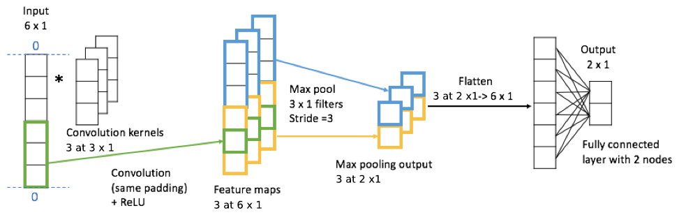
Convolutional neural network is a class of deep neural networks that uses the convolution operation to define the type of connections from one layer to another. While they have shown impressive results in extracting complex features from images in computer vision applications (Krizhevsky et al., 2012; Simonyan and Zisserman, 2015), they are relevant in many other applications involving structured input data, e.g., 1D sequences. A CNN is composed of an input layer, multiple hidden layers and an output layer. The hidden layers usually consist of several convolutional layers, followed by pooling layers, fully connected layers (dense layers) and normalization layers. Figure 1 shows a simple example of CNN. The input vector (or sequence) is first passed through a convolutional layer where it is convolved with three filters (convolution kernels) of size 3 using the same padding to produce three 6×1 feature maps. Since the rectified linear unit (ReLU) function, $f\left(\mathit{x}\right)=max(\mathrm{0},\mathit{x}$), is commonly chosen as the activation function in CNNs, the feature maps only contain positive values. Then the max pooling layer picks the maximum value every three elements for each feature map, generating three 2×1 vectors. After passing through a flattened layer, the max pooling output is reshaped into a 6×1 vector, which is followed by a dense (fully connected) layer with two nodes. The dense layer multiplies its input by a weight matrix and adds a bias vector for generating the output of the model. The computer adjusts the model's convolutional kernel values or weights through a training process called backpropagation, a class of algorithms utilizing the gradient of loss function to update weights. For the case in Fig. 1, there are 26 tunable parameters, i.e., $(\mathrm{3}+\mathrm{1})\times \mathrm{3}=\mathrm{12}$ from convolution kernels and $(\mathrm{6}+\mathrm{1})\times \mathrm{2}=\mathrm{14}$ from the dense layer.

LSTM neural networks have many applications such as speech recognition (Li and Wu, 2015) and handwriting recognition (Graves et al., 2008; Graves and Schmidhuber, 2009). They are a special kind of ANNs termed as recurrent neural networks (RNNs). RNNs are designed for modeling sequence-dependent behavior (e.g., in time). They are called “recurrent” because they perform the same operation for every element of a sequence, with the output at a given element dependent on previous computations at earlier elements (Britz, 2015). This is different from traditional neural networks wherein all the input–output examples are assumed to be independent of each other.

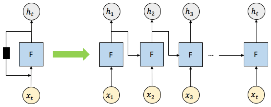
Figure 2 shows a diagram of an unrolled RNN with t input nodes, where “unrolled” means showing the network for the full sequence of inputs and outputs. The RNNs work as follows. At the first element of the sequence, the set of input signals x₁ (which can be multidimensional) is fed into the neural network F to produce an output h₁. At the next element of the sequence, the same neural network F takes both the next input x₂ and previous output h₁, generating the next output h₂. This recurrent computation continues for t times to produce the output at the tth element of the sequence, h_t. While RNNs are powerful architectures for modeling sequence behavior, classical RNNs are inadequate to capture long-term memory effects where the inputs–outputs at a given element of the sequence can affect the outputs at another element of the sequence separated by a long interval. LSTM models are variants of RNNs that are able to overcome this challenge and are efficient at capturing long-term dependencies as well as short-term dependencies. It does so by introducing an internal memory state that is operated by neural network layers termed as gates, such as the “input gate,” which adds new information from the input signals to the memory state, the “forgot gate,” which erases content from the memory state depending on the input signals, and the “output gate,” which transforms information contained in the input signals and the memory state to produce output signals.

Figure 2 Unrolled recurrent neural network.

An example of an LSTM cell is illustrated in Fig. 3, of which the update rules are as follows:

$$\begin{array}{c}{\displaystyle }{g}_j=\tanh \left(b^g+x_j{U}^g+h_{j-\mathrm{1}}{V}^g\right)\\ {\displaystyle }{i}_j=\mathit{\sigma }\left(b^i+x_j{U}^i+h_{j-\mathrm{1}}{V}^i\right)\\ {\displaystyle }{f}_j=\mathit{\sigma }\left(b^f+x_j{U}^f+h_{j-\mathrm{1}}{V}^f\right)\\ {\displaystyle }{s}_j=s_{j-\mathrm{1}}\circ f_j+g_j\circ i_j\\ {\displaystyle }{o}_j=\mathit{\sigma }\left(b^o+x_j{U}^o+h_{j-\mathrm{1}}{V}^o\right)\\ {\displaystyle }{h}_j=\tanh \left(s_j\right)\circ o_j,\end{array}$$

where j is the element index, σ(x) represents the sigmoid function, and tanh(x) represents the hyperbolic tangent function. x∘y denotes the element-wise product of x and y. U^g, Uⁱ, U^f and U^o are the weights for the input x_j, while V^g, Vⁱ, V^f and V^o are the weights for the other input h_j−1, and b^g, bⁱ, b^f and b^o are the scalar terms (termed as bias). The term g_j is the input modulation gate, which modulates the input $b^g+x_j{U}^g+h_{j-\mathrm{1}}{V}^g$ by a hyperbolic tangent function, squashing the input between −1 and 1. The term i_j is the input gate, which applies a sigmoid function to its input, limiting the output values to between 0 and 1. The input gate i_j determines which inputs are switched on or off when multiplying the modulated inputs (g_j∘i_j). The term s_j is the internal cell state that provides an internal recurrence loop to learn the sequence dependence. The terms f_j and o_j are the forgot gate and output gate, respectively. They have similar function to the input gate i_j, regulating the information into and out of the LSTM cell. The term h_j is the output at step j.

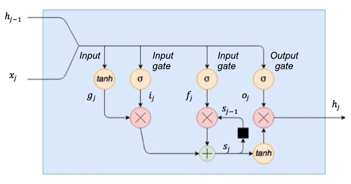
Figure 3 LSTM cell diagram (modified from Thomas, 2018).

2 Multi-axis differential optical absorption spectroscopy (MAX-DOAS) technique

The MAX-DOAS technique has been widely used to derive vertical aerosol extinction coefficient profiles in the lower troposphere. This is typically done from ground-based measurements of oxygen collision complex (O₂O₂) absorption (for a detailed list of references see Table 1 in Wagner et al., 2019). Since the oxygen volume mixing ratio (${\mathit{\chi }}_{{\mathrm{O}}_{\mathrm{2}}}=\mathrm{0.209}$) is considered constant, the O₂O₂ abundance depends only on the total number of air molecules (pressure, temperature and, to a small degree, humidity) and can be easily calculated. More than 93 % of O₂O₂ is located below 10 km (scale height ∼ 4 km). Any deviation in measured O₂O₂ absorption from this molecular (Rayleigh) scattering case is only due to the change in the photon path through the O₂O₂ layer. Aerosols and clouds are the main causes of such photon path modification for ground-based measurements. O₂O₂ has several absorption bands in the ultraviolet (UV) and visible (VIS) parts of the electromagnetic spectrum (band peaks at 343, 360, 380, 477, 577, 630 nm; Thalman and Volkamer, 2013).

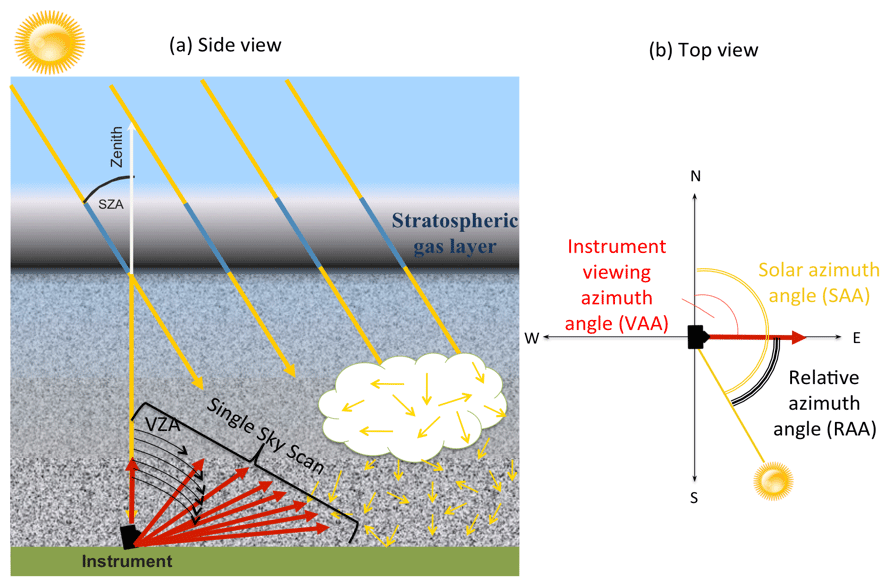
Figure 4 Demonstration of the MAX-DOAS principle: (a) side view and (b) top view. Simplified photon paths through the atmosphere are shown in yellow. A single sky scan sequence for profile retrieval consists of multiple viewing zenith angles (VZAs) in a specific direction (viewing azimuth angle, VAA) at a specific solar zenith angle (SZA) and is shown in red.

The MAX-DOAS technique consists of measuring sky-scattered UV–VIS solar photons at multiple, primarily, low elevation angles (Fig. 4). MAX-DOAS shows a large sensitivity to the tropospheric gases due to increased photon path length through the lower troposphere (Platt and Stutz, 2008). To eliminate the contribution from the upper-atmosphere, solar spectra measured at low elevation angles are divided by the reference spectrum collected from the zenith direction. The DOAS technique has the advantage of not needing an absolute radiometric calibration.

The first step of the DOAS retrieval is a spectral evaluation to calculate the differential slant column density ($\mathrm{\Delta }{\mathrm{SCD}}_{\mathrm{measured}}=\mathrm{SCD}-{\mathrm{SCD}}_{\mathrm{reference}}$) of O₂O₂. This step is accomplished through the simultaneous nonlinear least-squares fitting of the absorption by species i, low-order polynomial function (P_LO) and offset to the difference between the logarithms of the attenuated (I) and reference (I_reference) spectra (Eq. 1). P_LO estimates combined attenuation due to molecular scattering and aerosol total extinction (scattering and absorption). The offset term approximates instrumental stray light and residual dark current.

$$\begin{array}{}\text{(1)}& \begin{array}{rl}\ln \left(I_{\mathrm{reference}}\left(\mathit{\lambda }\right)\right)& -\ln \left(I\left(\mathit{\lambda }\right)-\mathrm{offset}\left(\mathit{\lambda }\right)\right)\\ & =\left(\sum _s{\mathit{\sigma }}_i\left(\mathit{\lambda }\right)\cdot \mathrm{\Delta }{\mathrm{SCD}}_i\right)+P_{\mathrm{LO}}\end{array}\end{array}$$

The second step of the MAX-DOAS analysis is the conversion of a single sky scan (multiple viewing angles) ΔSCD(O₂O₂) into a vertical aerosol extinction coefficient profile. The physical relationship between the measured ΔSCD and the desired aerosol extinction coefficient profile and aerosol properties is complex and, in general, can be expressed mathematically by Eq. (2) (Rodgers, 2004):

$$\begin{array}{}\text{(2)}& \mathit{y}=f\left(\mathit{x},\mathit{b}\right)+\mathit{\epsilon },\end{array}$$

where the measured quantities (measurement vector y) are described by a forward model f(x,b) and the measurement error vector (ε). The forward model, f(x,b), is a model that estimates physical processes that relate the measured parameter (y), the unknown quantity to be retrieved (state vector x), and forward model parameters (b) that are considered approximately known (e.g., temperature and pressure profiles from atmospheric soundings or models). Under most conditions, there are more unknowns than measurements, and as a result Eq. (2) does not have a unique solution.

The inversion of Eq. (2) is often done in the framework of Bayes' theorem, which allows for the assignment of probability density functions to all possible states given measurements and prior knowledge of the state. However, in reality, we are not interested in all possible solutions but rather a single, the most “probable” solution with its error estimation. Equation (3) shows a Transfer Function that defines an estimated solution ($\widehat{x}$) as a function of the measurement system and retrieval method (Rodgers, 2004) as follows:

$$\begin{array}{}\text{(3)}& \widehat{\mathit{x}}=R\left(f\left(\mathit{x},\mathit{b}\right)+\mathit{\epsilon },\widehat{\mathit{b}},{\mathit{x}}_a,\mathit{c}\right),\end{array}$$

where R is a retrieval method, f(x,b) is a forward function with the true state (x) and true parameters (b), $\widehat{\mathit{b}}$ is the estimated forward model parameter vector, x_a is the a priori estimate of state vector (x), and c is a retrieval method parameter vector (e.g. convergence criteria). For nonlinear problems the solution to Eq. (3) cannot be found explicitly, and iterative numerical methods are required. A maximum a posteriori (MAP) approach has been widely applied to moderately nonlinear problems with Gaussian distribution of both measurement errors and a priori state errors. A priori information about the state vector distribution before the measurements are made is used to constrain the solution of the ill-posed problems (Rodgers, 2004). It is essential to use the best estimate of the state available since in the MAP approach the retrieved state is proportional to the weighted mean of the actual state and the a priori state. In addition, an appropriate covariance matrix for the a priori state vector has to be constructed. This a priori information for aerosol vertical extinction coefficient profiles, however, is rarely available.

In addition to the optimal estimation method (OEM), briefly described above, parameterized (Beirle et al., 2019; Vlemmix et al., 2015) and analytic (Frieß et al., 2019; Spinei et al., 2020) inversion algorithms were developed. Frieß et al. (2019) provided a detailed intercomparison of currently available state-of-the-art inversion algorithms for the MAX-DOAS measurements. Most of the current algorithms take between 3 to 216 s to process a single MAX-DOAS sky scan (Frieß et al., 2019), mainly due to the iterative inversion step. Aerosol extinction coefficient profiles are inverted, while aerosol single-scattering albedo and asymmetry factor are typically assumed based on the colocated AERONET measurements. They also require external information about the atmosphere (e.g. temperature and pressure profiles) that might not be readily available at the measurement timescales and a priori information that does not typically exist. With an increasing number of MAX-DOAS 2D instruments worldwide capable of sunrise to sunset measurements (e.g. Pandonia Global Network), fast methods are needed that can harvest full information from the MAX-DOAS hyperspectral measurements.

This study describes and evaluates a fast novel machine learning (ML) approach for retrieving aerosol extinction coefficient profiles, asymmetry factor and single-scattering albedo at 360 nm from ΔSCD(O₂O₂) observations within a single MAX-DOAS sky scan. The basic idea of our approach is as follows: (1) develop an “inverse model” by one-time offline training of a supervised ML algorithm on simulated MAX-DOAS data and corresponding atmospheric aerosol conditions and (2) use the relationships derived in the first step to estimate the aerosol extinction profile, asymmetry factor and single-scattering albedo from the MAX-DOAS ΔSCD(O₂O₂) measurements. We specifically leverage recent advances in ML, e.g., deep learning methods, to automatically extract the inverse mapping from the observations (y) to the state vectors (x), using a collection of (x, y) pairs available for training. Different machine learning algorithms were successfully used in remote-sensing applications (Schulz et al., 2018; Schilling et al., 2018; Efremenko et al., 2017; Hedelt et al., 2019).

The rest of the paper is organized in the following sections. Section 3 provides an overview of the new retrieval algorithm. Section 4 focuses on training data generation using the radiative transfer model (Vector Linearized Discrete Ordinate Radiative Transfer, VLIDORT). Section 5 details ML implementation. Section 6 provides an extensive comparison of ML-predicted versus “true” macroscopic aerosol properties outside the training dataset. Section 7 summarizes the findings.

3 Overview of the methodology

Our approach consists of three stages: (1) training set generation; (2) a one-time training that results in an inverse ML model $R\left(\widehat{\mathrm{\Theta }}\right)$ with appropriate architecture and parameters $\widehat{\mathrm{\Theta }}$; and (3) an inversion stage, where the trained ML model $R\left(\widehat{\mathrm{\Theta }}\right)$ is applied to MAX-DOAS measurements to retrieve aerosol properties. Figure 5 provides a schematic overview of the three stages.

Figure 5 Schematics of the machine learning inversion algorithm.

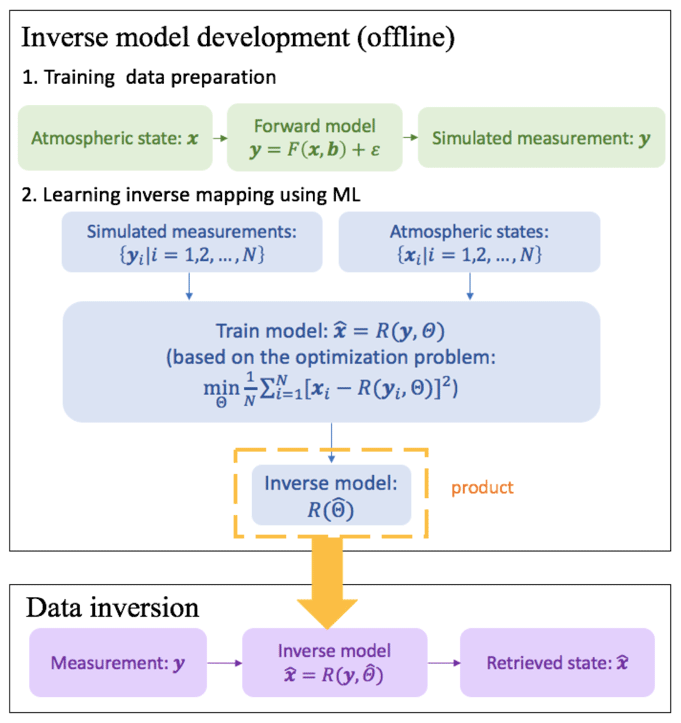
First, a training set containing simulated measurements $\mathit{\{}{\mathit{y}}_i\mathrm{|}i=\mathrm{1},\mathrm{2},\mathrm{\dots },M\mathit{\}}$ is generated by a forward model (VLIDORT v2.7) given atmospheric states $\mathit{\{}{\mathit{x}}_i\mathrm{|}i=\mathrm{1},\mathrm{2},\mathrm{\dots },N\mathit{\}}$. The model describes atmospheric radiative transfer processes connecting the atmospheric states and the measurements. Second, both the atmospheric states and the simulated measurements are fed into the ML model for learning the inverse mapping from the measurement space to the state space. This is based on solving an optimization problem that minimizes the mean squared error (MSE) between the retrieved values ($\mathit{\{}{\widehat{x}}_i\mathrm{|}i=\mathrm{1},\mathrm{2},\mathrm{\dots },N\mathit{\}}$) and the true values ($\mathit{\{}{\mathit{x}}_i\mathrm{|}i=\mathrm{1},\mathrm{2},\mathrm{\dots },N\mathit{\}}$). We specifically chose artificial neural network (ANN) models to learn the inverse mapping from y to x. By iteratively adjusting the parameters of the ANN model using gradient descent (backpropagation) algorithms (Johansson et al., 1991), we are able to arrive at ANN model parameters $\widehat{\mathrm{\Theta }}$ that provide a local optimum performance in terms of MSE on the training data. The result of the training stage is an inverse model $R(\widehat{\mathrm{\Theta }}$) whose architecture and parameters are saved in an HDF5 file (1.3 MB). The trained model $R\left(\widehat{\mathrm{\Theta }}\right)$ is an inversion operator that transforms measurements vector y into the state vector $\widehat{x}$ through a set of simple linear and nonlinear operations. The inverse model provides a convenient and fast way for retrieval of aerosol properties from ΔSCD(O₂O₂) measurements during the inversion stage. It takes ∼ 0.15 ms for the retrieval of the studied aerosol properties from a single MAX-DOAS sky scan ΔSCD(O₂O₂) on a single CPU core.

4 Training data preparation

The success of any ML model depends on the quality of the training data. Since there is no reliable dataset that combines simultaneous MAX-DOAS measurements and observations of aerosol macrophysical properties and vertical extinction coefficient profiles at 360 nm, we use a radiative transfer model to simulate MAX-DOAS measurements. In this study, we train our ML model on air mass factors (AMF) calculated from the simulated solar radiances at the bottom of the atmosphere.

AMF represents a ratio between the true average path that photons take through a gas layer before detection by a MAX-DOAS instrument and the vertical path. Since O₂O₂ absorption in the reference (zenith scattered) spectrum is not precisely known, a differential AMF at a specific wavelength λ and observations geometry μ (relative azimuth angle, solar zenith angle and viewing zenith angle) is determined as follows:

$$\begin{array}{}\text{(4)}& \begin{array}{rl}\mathrm{\Delta }\mathrm{AMF}\left({\mathrm{O}}_{\mathrm{2}}{\mathrm{O}}_{\mathrm{2}},\mathit{\lambda },\mathit{\mu }\right)& ={\displaystyle \frac{\mathrm{\Delta }{\mathrm{SCD}}_{\mathrm{measured}}\left({\mathrm{O}}_{\mathrm{2}}{\mathrm{O}}_{\mathrm{2}},\mathit{\lambda },\mathit{\mu }\right)}{\mathrm{VCD}({\mathrm{O}}_{\mathrm{2}}{\mathrm{O}}_{\mathrm{2}}{)}_{\mathrm{calculated}}}}\\ & ={\displaystyle \frac{\ln \left(I_{\mathrm{reference}}\left(\mathit{\lambda },{\mathit{\mu }}_o\right)\right)-\ln \left(I\left(\mathit{\lambda },\mathit{\mu }\right)\right)}{\mathrm{VCD}({\mathrm{O}}_{\mathrm{2}}{\mathrm{O}}_{\mathrm{2}}{)}_{\mathrm{calculated}}\cdot \mathit{\sigma }\left({\mathrm{O}}_{\mathrm{2}}{\mathrm{O}}_{\mathrm{2}},\mathit{\lambda }\right)}},\end{array}\end{array}$$

where vertical column density of O₂O₂ (VCD) is estimated as the squared oxygen number density integrated from the surface to the top of the atmosphere; and σ(λ) is the molecular absorption cross section of O₂O₂.

Table 1 Radiative transfer model settings.

In the absence of aerosols and clouds, only air molecules (mainly oxygen and nitrogen) scatter solar photons in the Earth's atmosphere. This molecular-only (Rayleigh) scattering process is considered to be well understood (Bodhaine et al., 1999), and ΔAMF^Rayleigh can be calculated from the simulated intensities. In the presence of aerosols, dust and clouds, not only air molecules but also particles and cloud droplets scatter solar photons. This type of scattering can be generally described by the T-matrix theory. In this study we consider only spherical aerosols (Lorenz–Mie theory), whose scattering phase function is approximated according to the Henyey–Greenstein approach using the asymmetry factor g. ΔAMF^{aerosol+Rayleigh} are determined from simulated downwelling radiances for atmosphere with different aerosol types and their extinction coefficient profiles. The change in AMF due to aerosol presence can be described by ΔAMF^aerosol:

$$\begin{array}{}\text{(5)}& \mathrm{\Delta }{\mathrm{AMF}}^{\mathrm{aerosol}}=\mathrm{\Delta }{\mathrm{AMF}}^{\mathrm{Rayleigh}}-\mathrm{\Delta }{\mathrm{AMF}}^{\mathrm{aerosol}+\mathrm{Rayleigh}}.\end{array}$$

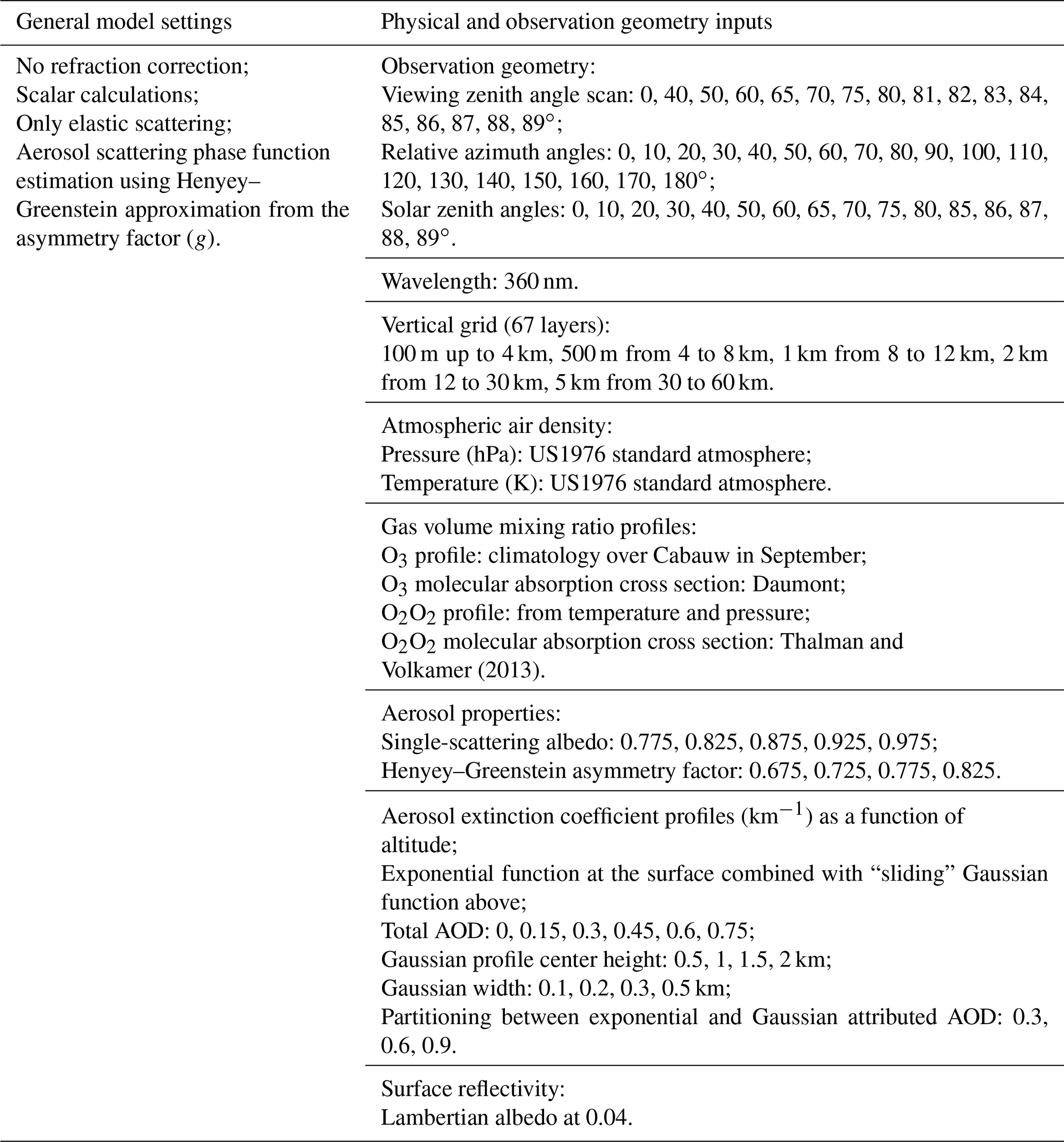
ΔAMF^aerosol for O₂O₂ at 360 nm for different observation geometries and scattering conditions is used for ML training in this feasibility study. A single MAX-DOAS measurement considered here is ΔAMF^aerosol set from the full sky scan at a single solar zenith angle, single relative azimuth angles, and 19 viewing zenith angles between 0 and 89^∘ (see Table 1). To ensure that the training dataset contains all observation geometries feasible for MAX-DOAS sky scans we have included 19 relative azimuth angles (0 to 180^∘, 10^∘ step) and 12 solar zenith angles (0 to 85^∘ – see Table 1). Solar radiances at the bottom of the atmosphere were simulated using VLIDORT v.2.7 (Spurr, 2008). VLIDORT is a discrete-ordinate radiative transfer model that has been successfully applied to simulate radiances and weighting functions for forward models in optimal estimation inversion (e.g., Clémer et al., 2010) and machine learning algorithms (Efremenko et al., 2017; Hedelt et al., 2019). VLIDORT code applies pseudo-spherical approximation to direct solar beam attenuation in a curved atmosphere. All scattering processes are estimated using the plane-parallel approximation in a stratified atmosphere. Precise single-scattering computation is performed using Nakajima–Tanaka ansatz and delta-M scaling. VLIDORT v.2.7 calculates analytically derived Jacobians (radiance weighting functions) with respect to any profile/column/surface variables. VLIDORT computes elastic scattering by molecules to all orders (Spurr, 2008).

VLIDORT models radiative transfer processes at a specific wavelength in a stratified atmosphere. It requires geometrical and “optical” information about the atmospheric layers and the underlying ground surface. These include layer heights, pressure and temperature at layer boundaries for refractive geometry calculations, solar zenith, viewing zenith direction, and relative azimuth angles between the viewing direction and solar position. Each atmospheric layer is described by total optical thickness, total single-scattering albedo and the set of Greek matrices specifying the total scattering law.

VLIDORT simulations were performed for the US 1976 standard atmosphere divided into 67 layers (same as in Frieß et al., 2019) with 0.1 km layers from the surface to 4 km; 0.5 km layers from 4 to 8 km and varying width up to 60 km. Since surface reflectivity has a small effect on ground-based MAX-DOAS measurements we performed simulations only for a single Lambertian albedo of 0.04. Absorption only by two gases was considered in this study: ozone and O₂O₂. Light polarization, direct beam refraction and inelastic scattering were not included in this study. Table 1 summarizes VLIDORT inputs and general settings.

Aerosol types in this study are described by a single-scattering albedo and asymmetry factor combination with a total of 20 “types”: (1) single-scattering albedo: 0.775, 0.825, 0.875, 0.925, 0.975; (2) Henyey–Greenstein asymmetry factor: 0.675, 0.725, 0.775, 0.825. Aerosol extinction coefficient profiles were generated by combining an exponential function at the surface with a “sliding” Gaussian function above. The aerosol total optical depth was partitioned between the exponential and Gaussian functions. Total AOD cases included 0.15, 0.3, 0.45, 0.6 and 0.75 with exponential-to-Gaussian partitioning fractions of 0.3, 0.6 and 0.9. The Gaussian function peak center height was varied from 0.5 to 2 km in steps of 0.5 km. The Gaussian function peak width was varied too, at 0.1, 0.2, 0.3 and 0.5 km. This results in 4800 aerosol cases and a total of 1 459 200 measurement simulations (sky scan). Figure 14 demonstrates the aerosol profile samples, where the near-surface aerosol partial optical depth profiles are described by the exponential function, and the layers aloft are described by the Gaussian function with various widths and heights added to the exponential function profile. While VLIDORT simulations were performed for an atmosphere divided into 67 layers, ML training was done by resampling only onto 23 layers. The new layer depths are 100 m from the surface to 1 km, 200 m from 1 to 3 km, 500 m from 3 to 4 km, and 56 km (height of the last layer). The new layer partial AODs were generated by adding the neighboring layer partial aerosol optical depths. The ML algorithm was trained on 75 % randomly selected measurement simulations (1 094 400 samples), and model performance was tested on the remaining 25 %. Note that no validation data were held off from the 75 % training set for tuning hyperparameters of our ML model, as all ML hyperparameters were kept constant across all experimental settings in this paper.

5 Learning inverse mapping using ML

We employ a supervised ML formulation for our problem of aerosol profile retrieval, where the goal is to learn the mapping from input variables to output variables given a training set of paired data instances. In our formulation, every data instance corresponds to a single MAX-DOAS sky scan at a fixed relative azimuth angle (RAA) and solar zenith angle (SZA), where the inputs of the data instance comprise the following: (a) RAA scalar value, (b) SZA scalar value and (c) a sequence of ΔAMF^aerosol values at 16 VZAs. The output variables at a data instance correspond to the aerosol properties we are interested in predicting given the inputs, which are as follows: (a) single-scattering albedo (SSA) scalar value; (b) asymmetry factor (ASY) scalar value; and (c) a sequence of partial aerosol optical depth (AOD) values at 23 vertical layers of the atmosphere, termed as the aerosol extinction profile.

Note that in our supervised ML formulation, there are sequences in both the input signals and output signals, namely ΔAMF^aerosol sequence and partial AOD sequence, respectively. Further note that the input and output signals used in our problem setting are of very different types and thus have different dimensionalities (e.g., ΔAMF^aerosol takes 16 values at varying VZAs, while partial AOD takes 23 values at varying atmospheric layers). We thus first apply a 1D CNN to extract features from the sequence part of the input signals. Note that our input signals are not image based, which is one of the common types of input data for which CNNs are used. Instead, our input data are structured as a 1D sequence, and the convolution operations of CNN help in extracting sequence-based features from the input signals that are then fed into subsequent ANN components. We also use an LSTM to model the sequence part of the output signals. Note that our data contain no time dimension as we are only working with single-scan data, assuming the atmosphere does not change during the scan time. However, it is the sequence-based nature of the output signals that motivated us to use LSTM models for sequence-based output prediction. Furthermore, the dataset we use for training is produced by a physical model (VLIDORT), where the relationship between the inputs and outputs are known.

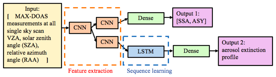
Figure 6 Schematics of the multi-output sequence-to-sequence model for deriving aerosol optical properties from MAX-DOAS measurements.

Figure 6 illustrates the novel multi-output sequence-to-sequence model for learning the inverse mapping from MAX-DOAS measurements to aerosol optical properties. To extract sequence-based features from MAX-DOAS inputs, a 1D convolutional neural network (CNN; Fukushima, 1980; LeCun et al., 1999) is first applied to the sequence of inputs (we concatenate ΔAMF^aerosol sequence with SZA and RAA to obtain an input sequence of length 18), which results in a sequence of preliminary hidden features. These preliminary hidden features are then sent to two different branches of 1D CNN layers that perform further compositions of convolution operators to produce nonlinear hidden features for predicting two different types of outputs: (a) scalar outputs: SSA and ASY; and (b) sequence-based outputs: aerosol extinction profile. For the branch corresponding to scalar outputs, the features extracted from 1D CNN layers are simply passed on to a fully connected dense layer to produce a 2D output of SSA and ASY. For the branch corresponding to sequence-based outputs, the features extracted from 1D CNN layers are fed to a long short-term memory network (LSTM; Hochreiter and Schmidhuber, 1997) to produce a sequence of partial AOD values at varying atmospheric layers.

Figure S1 in the Supplement shows the detailed architecture of the multi-output sequence-to-sequence model. The CNNs consist of eight 1D convolutional layers (c₁ to c₈) and four max-pooling layers (p₁ to p₄). For convolutional layers c₁ to c₆, the activation function is the rectified linear unit (ReLU) function. For layers c₇ and c₈, it is a hyperbolic tangent function (tanh). We set the kernel size of the convolution operation to be the typical value of 5 and use the same padding for all $c_k\forall k\in \mathit{\{}\mathrm{1},\mathrm{2},\mathrm{\dots },\mathrm{8}\mathit{\}}$. ReLU and max pooling layers help to reduce overfitting through model sparsity and parameter reduction. The convolution kernel weights are initialized using a “Glorot uniform” method (Glorot  and Bengio, 2010).

Extracted feature vector from the p₁ layer is sent into two different branches. In the branch for profile prediction, we take a one-to-many LSTM with 23 layer steps and a hidden size of 128 to capture the correlation between the partial AODs at different layers. We simply duplicate the feature vector learned from CNNs 23 times to generate the inputs for the LSTM model. The sequential output $\mathit{\{}{y}_{\mathrm{1}},y_{\mathrm{2}},\mathrm{\dots },y_{\mathrm{23}}\mathit{\}}$ of the LSTM (after passing through a flattened layer and an ReLU layer) is interpreted as the 23-layer aerosol extinction profile. For the SSA–ASY branch, 1D convolutional layers and dense layers are combined for the prediction. The reason for taking a two-output architecture is that SSA and ASY are independent scalar outputs that cannot be treated as a sequence, in contrast to the aerosol extinction profile.

We implemented our ML model in the Jupyter notebook using the Keras library, which is a commonly used deep learning library for Python. RMSprop was chosen as the optimizer, and the mean squared error was used as the loss function (Hinton, 2012). We trained the model on 75 % of the dataset for 124 epochs with a batch size of 640. The following choice of hyperparameters was used: choice of optimizer is RMSprop, with a learning rate of 0.001, a decay factor of 0.9, a learning rate decay of 0 and a fuzz factor – none. We did not perform any hyperparameter tuning on a separately held validation set inside the training set, and the values of all hyperparameters in our ML model were kept constant throughout all experiments in the paper on the test set. In order to ensure that there was no overlap between the training and testing steps, we did not make use of the test data either directly or indirectly during the training phase, either for learning parameter weights or selecting hyperparameters.

6 Results

Evaluation of the accuracy of ML mapping rules derived during the training stage for MAX-DOAS data inversion was done by comparing the true atmospheric aerosol properties to the ML inverted properties. The evaluation dataset consists of 364 800 MAX-DOAS simulated sky scans that are outside of the training set. The number of simulations in the evaluation dataset as a function of solar zenith angle (SZA) and relative azimuth angle (RAA) are shown in Fig. 7. Between 1100 and 1300 aerosol scenarios are present in each SZA-RAA bin.

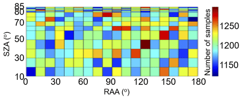
Figure 7 Number of simulations in the evaluation dataset as a function of solar zenith (SZA) angle and relative azimuth angle (RAA).

The following ML-predicted aerosol properties were evaluated: (1) asymmetry factor, (2) single-scattering albedo, (3) total aerosol optical thickness and (4) partial aerosol optical thickness for each layer from 0 to 4 km. A relative error ϵ of the retrieved by ML parameter $\widehat{x}$ relative to the true value x is calculated according to Eq. (6):

$$\begin{array}{}\text{(6)}& \mathit{ϵ}\equiv {\displaystyle \frac{\widehat{x}-x}{x}}\cdot \mathrm{100}\mathit{\%}.\end{array}$$

The relative error evaluation presented in the subsequent sections was performed on the retrievals from a single ML training. Since ML itself introduces randomness during the training stage, we retrained the model 20 times with the same hyperparameters for evaluating the uncertainty in the ML training.

6.1 Asymmetry factor at 360 nm

The ML-based approach shows an ability to invert aerosol asymmetry factor with a mean error of −0.14 % and 2 standard deviations of 2.04 % and nearly normal error distribution (Fig. 8a). To evaluate if any dependence of the asymmetry factor retrieval exists on SZA and RAA, the mean error and the 2 standard deviations are shown in Fig. 8b, c. These distributions suggest that dependence of the asymmetry factor retrieval on SZAs and RAAs is relatively small. However, systematically higher relative errors are observed around SZA of 65^∘ and RAA of 30–40^∘. The cause of these elevated errors is not clear at this point.

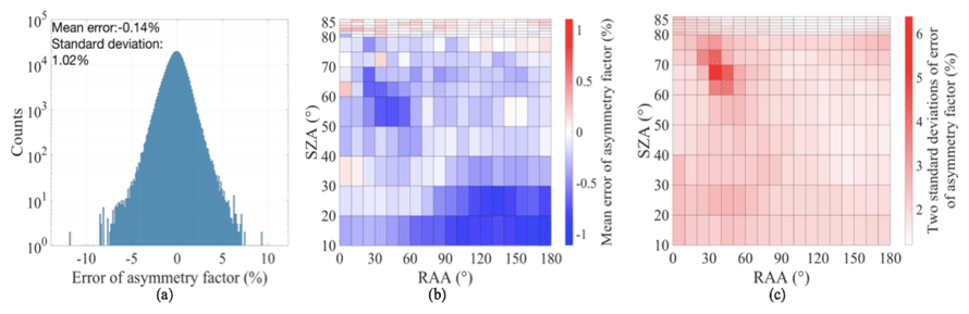
Figure 8 Asymmetry factor retrieval errors: (a) error histogram; (b) mean error as a function of SZA and RAA; (c) 2 standard deviations as a function of SZA and RAA.

Figure 9 Single-scattering albedo retrieval errors: (a) error histogram, (b) mean error as a function of SZA and RAA, and (c) 2 standard deviations as a function of SZA and RAA.

6.2 Single-scattering albedo at 360 nm

Similar high accuracy is achieved for ML retrieval of the single-scattering albedo with a mean error of 0.19 % and 2 standard deviations of 3.46 % and nearly normal error distribution, somewhat positively skewed (Fig. 9). Slightly higher errors are observed at RAA smaller than 60^∘ and most SZA.

Mean errors are also larger at small RAA and SZA >85^∘. Traditional optimal estimation techniques also struggle with the MAX-DOAS data inversion at small RAA due to uncertainty in aerosol forward and backward scattering.

6.3 Total aerosol optical depth at 360 nm

Total AOD retrieval is more challenging for the ML model than the single-scattering albedo or asymmetry factor, especially at lower total AOD levels. Boxplots of the total AOD error for different true total AOD values are given in Fig. 10. In general, the ML algorithm tends to underestimate total AOD from the mean error ±2 standard deviations of $-\mathrm{8.39}\pm \mathrm{8.81}$ % (total AOD 0.15) to $-\mathrm{1.52}\pm \mathrm{3.10}$ % (total AOD of 0.75). Total AOD retrieval error distribution over all cases is close to a Gaussian distribution but with two peaks (Fig. 11). The mean error (±2 standard deviations) is $-\mathrm{3.58}\mathit{\%}\pm \mathrm{7.68}$ %. The bias of the model does not have much dependence on SZAs and RAAs (Fig. 11b). Still, larger errors and uncertainties can be observed at higher SZAs and lower RAAs (Fig. 11c).

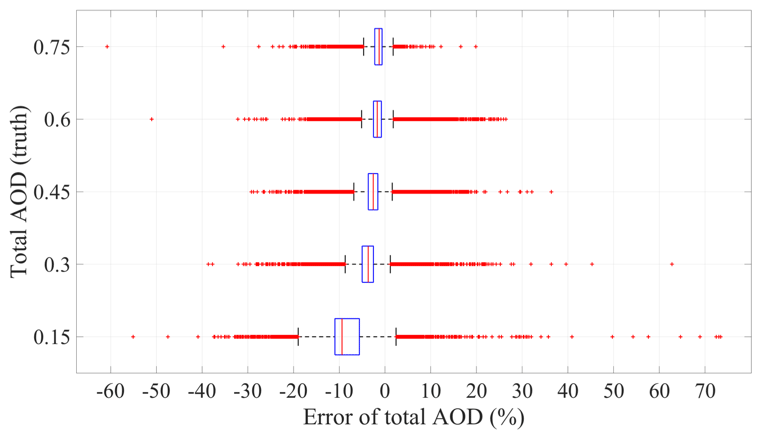
Figure 10 Boxplots of total AOD prediction errors for each true total AOD value. The box central mark indicates the median, and the bottom and top edges of the box indicate the 25th and 75th percentiles, respectively. The whiskers extend to the most extreme data points not considered outliers, and the outliers are plotted individually using the “+” symbol.

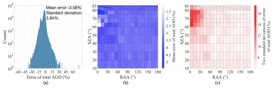
Figure 11 Total AOD retrieval errors: (a) error histogram, (b) mean error as a function of SZA and RAA, and (c) 2 standard deviations as a function of SZA and RAA.

6.4 Partial aerosol optical depth profile from 0 to 4 km

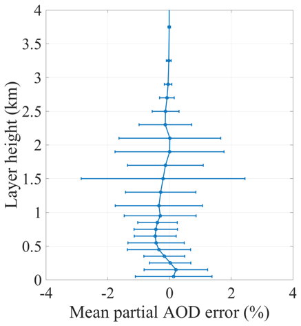
The contribution of partial AOD retrieval error at each atmospheric layer from 0 to 4 km to the total AOD is shown in Fig. 12. Layer partial AOD retrieval error relative to the total AOD depends on the absolute amount of aerosols and its altitude and on average is less than 1 % per layer. Just like OEM methods, the ML method has lower accuracy of retrieving elevated aerosol layers especially corresponding to smaller total AOD. The larger distribution of relative errors in partial AOD at 1.5 and 2 km is mainly due to the presence of elevated layers in the training data that peaked at those heights. If the aerosol were also present in meaningful amounts above those altitudes, the error distribution would have been larger above 2 km.

Figure 12 Mean partial layer AOD error ± 1 standard deviation.

A linear regression analysis of the true versus the retrieved partial AOD was performed using the least-squares fitting for each layer from 0 to 2.2 km (Fig. 13). Intercepts of linear regression analysis for all layers were zero with RMS≤0.01. High R² values (0.93–0.99) and slopes (m) close to one suggest that the ML method relatively accurately estimates partial AOD at the layers between 0 and 2.2 km. As was noted earlier lower retrieval accuracy is observed at the higher altitudes.

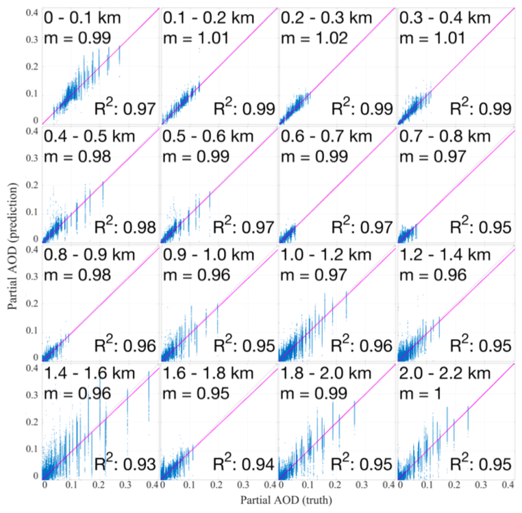
Figure 13 Correlation between the retrieved partial AOD and the true partial AOD for each layer from 0 to 2.2 km ($\text{retrieved partial AOD}=m\cdot \text{true partial AOD}+\text{intercept}$). The intercept of all linear regression analyses is 0 with RMS <0.01.

Figure 14 shows some examples of the partial AOD profiles retrieved by the ML inversion model. Panels (a)–(h) in Fig. 14 contain randomly selected profiles out of the tested pool. While panels (i)–(l) contain some of the worst predictions. These examples show that the ML model is able to predict the elevated aerosol layers and even in those cases having large discrepancies, the model is still capturing the correct shape.

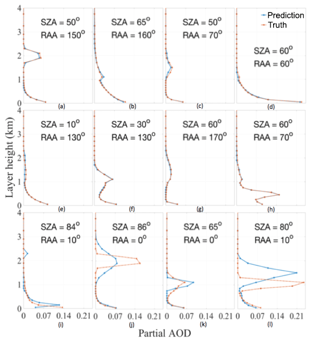
Figure 14 Examples of predicted partial layer AOD profiles: (a–h) randomly selected examples and (i–l) bad predictions.

6.5 Effect of random noise in ML training on the retrievals

To estimate retrieval uncertainties due to random noise in ML training on the aerosol properties we reran the ML training stage 20 times. Mean errors and standard deviations for total AOD, single-scattering albedo and asymmetry factor for each trained model are shown in Fig. 15.

Figure 15 Effect of random noise in model training on the retrieved aerosol properties.

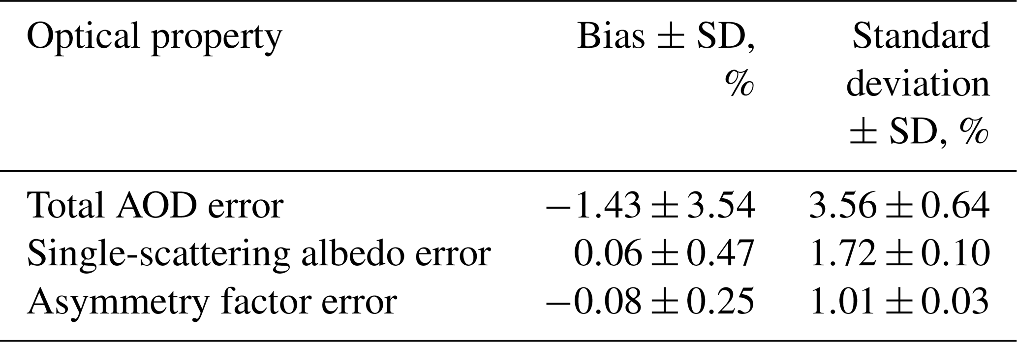
Table 2 summarizes the effect of random model training noise on the retrieved properties. In general, most ML models result in a normal distribution of errors with an additional bias in the mean. Since the individual model training has a very small effect on error distribution (small changes in standard deviation between the different training runs) we add the variation in bias with standard deviation in quadrature to estimate the total error of the ML model including the random error of the training as follows:

1. Total AOD error ±2 standard deviations $=-\mathrm{1.4}\pm \mathrm{10.1}$ %;

2. Single-scattering albedo error ±2 standard deviations $=\mathrm{0.1}\pm \mathrm{3.6}$ %;

3. Asymmetry factor error ±2 standard deviations $=-\mathrm{0.1}\pm \mathrm{2.1}$ %.

Table 2 Statistics of aerosol property error analysis from 20 ML models (20 different training runs).

7 Conclusions and future work

This paper presents a fast ML-based algorithm for the inversion of ΔSCD(O₂O₂) from a single MAX-DOAS sky scan into aerosol partial optical depth profile, single-scattering albedo and asymmetry factor at 360 nm. Training and evaluation of the ML algorithm are performed using VLIDORT simulations of ΔAMF(O₂O₂) for about 1.45 million scenarios with 75 % randomly selected cases for training and 25 % (∼ 365 000 cases) for evaluation.

Evaluation of four retrieved aerosol properties (asymmetry factor, single-scattering albedo, total AOD and partial AOD for each layer from 0 to 4 km) shows good performance of the ML algorithm with small biases and a normal distribution of the errors. Overall, 95.4 % of the retrieved optical properties have errors within the following ranges: ($-\mathrm{1.4}\pm \mathrm{10.1}$) % for total AOD, (0.1±3.6) % for single-scattering albedo and ($-\mathrm{0.1}\pm \mathrm{2.1}$) % for asymmetry factor. Linear regression analysis using the least-squares fitting method between the true and retrieved layer partial AODs resulted in high correlation coefficients (R²=0.93–0.99), slopes near unity (0.95–1.02) and zero intercepts with RMS≤0.01 for each layer from 0 to 2.2 km. The ML algorithm, in general, has less accuracy retrieving low total AOD scenarios and their corresponding profiles. Even in those scenarios with less accuracy, the ML model is still capable of capturing the correct profile shape.

Application of ML-based algorithm to real data inversion has the following advantages:

1. Fast real-time data inversion of the aerosol optical properties;

2. Simple implementation by using an HDF file with the model coefficients in open-source codes such as Python;

3. Ability to retrieve single-scattering albedo and asymmetry factor;

4. Use of the ML algorithm-retrieved aerosol extinction coefficient profiles; single-scattering albedo and asymmetry factor as initial guess inputs in more formal inversion algorithms (with radiative transfer simulations).

To verify that the ML retrievals are representative of the physical processes, we suggest simulating ΔSCD(O₂O₂) using a radiative transfer model (e.g., VLIDORT) with the ML-retrieved properties as inputs (aerosol extinction coefficient profile, single-scattering albedo, and asymmetry). Deviations from the measured and simulated ΔSCD(O₂O₂) should be included in error analysis.

To make the ML model more robust, the training data should include more realistic aerosol inputs and radiative transfer simulations including (1) rotational Raman scattering simulations to add ring measurements from MAX-DOAS, (2) different surface albedos, (3) more realistic aerosol profiles (e.g., from a 3D multiwavelength aerosol/cloud database based on CALIPSO and EARLINET aerosol profiles, LIVAS; Amiridis et al., 2015) and (4) multiple wavelengths.