the Creative Commons Attribution 4.0 License.
the Creative Commons Attribution 4.0 License.
 | 30 Oct 2020
Commercial microwave links as a tool for operational rainfall monitoring in Northern Italy
Giacomo Roversi
Pier Paolo Alberoni
Anna Fornasiero
There is a growing interest in emerging opportunistic sensors for precipitation, motivated by the need to improve its quantitative estimates at the ground. The scope of this work is to present a preliminary assessment of the accuracy of commercial microwave link (CML) retrieved rainfall rates in Northern Italy. The CML product, obtained by the open-source RAINLINK software package, is evaluated on different scales (single link, 5 km×5 km grid, river basin) against the precipitation products operationally used at Arpae-SIMC, the regional weather service of Emilia-Romagna, in Northern Italy. The results of the 15 min single-link validation with nearby rain gauges show high variability, which can be caused by the complex physiography and precipitation patterns. Known sources of errors (e.g. the attenuation caused by the wetting of the antennas or random fluctuations in the baseline) are particularly hard to mitigate in these conditions without a specific calibration, which has not been implemented. However, hourly cumulated spatially interpolated CML rainfall maps, validated with respect to the established regional gauge-based reference, show similar performance (R2 of 0.46 and coefficient of variation, CV, of 0.78) to adjusted radar-based precipitation gridded products and better performance than satellite-based ones. Performance improves when basin-scale total precipitation amounts are considered (R2 of 0.83 and CV of 0.48). Avoiding regional-specific calibration therefore does not preclude the algorithm from working but has some limitations in probability of detection (POD) and accuracy. A widespread underestimation is evident at both the grid box scale (mean error of −0.26) and the basin scale (multiplicative bias of 0.7), while the number of false alarms is generally low and becomes even lower as link coverage increases. Also taking into account delays in the availability of the data (latency of 0.33 h for CML against 1 h for the adjusted radar and 24 h for the quality-controlled rain gauges), CML appears as a valuable data source in particular from a local operational framework perspective. Finally, results show complementary strengths for CMLs and radars, encouraging joint exploitation.
- Article
(3448 KB) - Full-text XML
-
Supplement
(1040 KB) - BibTeX
- EndNote


High spatial and temporal variability make precipitation one of the most difficult geophysical observables to measure and monitor. Its accurate measurement would benefit a wide range of applications in meteorology, hydrology, climatology, and agriculture, just to name the most directly related fields where rainfall plays a key role. The precipitation rate can be measured or estimated directly at the ground or using different remote sensing approaches. Rain gauge networks provide point-like measurements of the amount of rain that has fallen within the instrument's sampling area, cumulated over time intervals which usually range from 1 min to 1 d, with well-known instrumental constraints (Lanza and Stagi, 2012) and representativeness limitations (Porcù et al., 2014). Ground-based weather radars, often deployed in large-scale networks (Serafin and Wilson, 2000; Huuskonen et al., 2014; Saltikoff et al., 2019), are widely used by hydrometeorological services to quantitatively monitor precipitation fields, being an effective trade-off between spatial temporal coverage and accuracy in the measurements. However, radar estimates are affected by several errors, which the last generation of polarimetric systems have only partially mitigated (Figueras i Ventura et al., 2012; Gou et al., 2019). Satellite estimates have received a renewed boost in the last decade from the full exploitation of the Global Precipitation Measurement (GPM) mission (Skofronick-Jackson et al., 2017) that has operationally released a new suite of precipitation products with a high temporal and spatial resolution (Mugnai et al., 2013; Grecu et al., 2016). Despite the undoubted potential of satellite products to provide estimates over open oceans and regions not equipped with ground instruments, their accuracy is difficult to assess at high spatial and temporal scales (Tang et al., 2020), and their latency hinders a real-time use.
A relatively new and independent approach to the estimate of precipitation at the ground has become available in the last few decades thanks to the growing number of microwave links (or commercial microwave links, CMLs) employed for the backhauling of cellular communication networks, growth which only recently and only in some densely populated areas seems to have come to a halt. Integrated precipitation content along a straight path between two antennas can be estimated by measuring the attenuation of the microwave signal travelling down the same path (Turner and Turner, 1970; Harden et al., 1978). Accurate experiments with dedicated hardware and numerical simulation were used to assess the capability of microwave links to measure average rainfall rates (Rahimi et al., 2003), drop size distribution (Rincon and Lang, 2002; van Leth et al., 2020), and water content (Jameson, 1993). The possibility of having a spatially continuous rainfall field depends on the density and distribution of the links, making the CML approach of particular interest for urban areas (Upton et al., 2005; Overeem et al., 2011; Fenicia et al., 2012; Fencl et al., 2013; Rios Gaona et al., 2018; de Vos et al., 2018) also with direct hydrological use in combination with conventional instruments (Grum et al., 2005; Fencl et al., 2013). A further application of the CML approach could be in regions where other instruments are lacking or entirely absent (Mulangu and Afullo, 2009; Abdulrahman et al., 2011; Doumounia et al., 2014). However, as happens for conventional precipitation instruments, the quality of the retrieval is sensitive to several factors, which are often difficult to control (Leijnse et al., 2008), and to the precipitation's microphysical structure (Berne and Uijlenhoet, 2007; Leijnse et al., 2010). Given these limitations intrinsic to the measurement geometry and to the nature of precipitation, possible synergistic approaches are considered to minimize the uncertainties of the different instruments, suggesting the potential of blending CML measurements with conventional precipitation estimates, such as rain gauges (Fencl et al., 2017; Haese et al., 2017), radar (Cummings et al., 2009; de Vos et al., 2019), or both (Grum et al., 2005; Bianchi et al., 2013).
Even if the general relationship between signal attenuation and rain rate is already well established, the successful use of CML data to quantitatively monitor precipitation still depends on the quality and technical characteristics of the transmitted power data and on the fine-tuning of the algorithms. The somewhat standardized policies of acquisition and storage of the different companies in different countries make the use of CMLs feasible all around the world, but there is as yet no standard way to access them as scientific data. As they consist mostly of confidential maintenance data, major obstacles to face are the widespread unwillingness of releasing them cost-free and inadequate data-quality standards (Chwala and Kunstmann, 2019).
The first objective of the present work is to make a validation of the precipitation amounts and distributions estimated only from CML attenuation data, using a well-established, freely available algorithm (i.e. RAINLINK; Overeem et al., 2016a), over two areas of interest in the Po Valley (provinces of Bologna and Parma), where CML data have been obtained from Vodafone (by direct purchase). Both areas contain river basins of considerable local interest, which will be explicitly addressed. Moreover, we consider for intercomparison only precipitation products routinely available at the Meteorological Service of the Regional Agency for Environmental Protection and Energy (Arpae-SIMC); this, on the one hand, prevents us from performing a solid calibration of the algorithm (see Sect. 3.2), but, on the other hand, allows us to understand how CML product behaves with respect to other operational products. The further aim of the validation study is thus to test the potential of the technology even at its most basic implementation, indicating where to direct the tuning efforts and setting the background for possible inclusion of CML data in the operational routine procedures for precipitation monitoring.
In Sect. 2 we will describe the area of interest and the different rainfall datasets (CML, radar, and rain gauges), including data quality and coverage. In Sect. 3 we will describe the RAINLINK algorithm and discuss its application to the Emilia-Romagna area. The comparison – at single-link and gridded-map scales – between the rainfall estimates from the different data sources is presented in Sect. 4 and discussed in Sect. 5, while conclusions are provided in Sect. 6.
We have considered 57 d from 5 May to 30 June 2016. The two target areas for which we have available CML data are the provinces of Bologna (BO, 3702 km2) and Parma (PR, 3447 km2), both in the Po Valley in Emilia-Romagna, Northern Italy (coloured areas in Fig. 1). The physiography of the two regions is similar: the highest peaks (about 1500 m a.s.l.) are located on the southern border, in the Apennine chain, while the central and northern parts of the two areas are flat land. The two river basins (thick lines in Fig. 1) are both located in the hilly region and have their closing sections located near the cities, in densely populated and asset-rich areas.
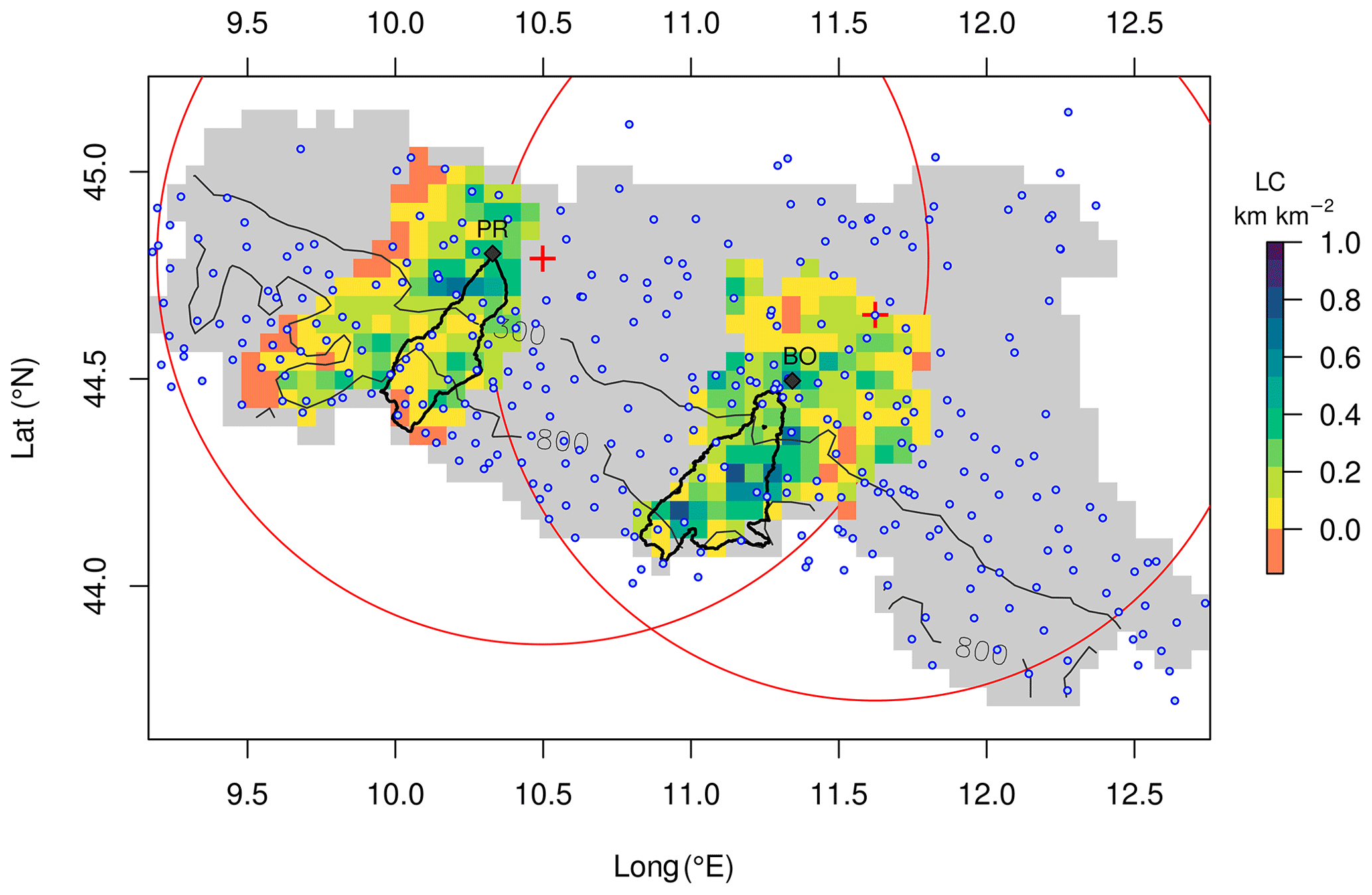
Figure 1Map of the Emilia-Romagna region in Northern Italy (grey area). The coloured areas are the two provinces where the CML estimates are computed (the colour scale represents the link coverage, LC, where orange is not a negative value but exactly zero), and thick black lines delimit the two river basins (Parma, to the east, and Reno). Blue circles and red crosses indicate operational rain gauge and weather radar locations, respectively, while red circles are the 100 km radar coverage. Thin black lines show two elevation contours (300 and 800 m a.s.l.). The capital cities of the two areas (Bologna – BO – and Parma – PR) are indicated with the black diamonds.
Precipitation climatology in the Po Valley during the late spring season is characterized by both stratified structures and small-scale convection, with the maxima of the rainfall amounts located on the Apennines ridge (see Supplement). We divided the whole area into square boxes of 5 km×5 km (see also Sect. 2.2.2), and this grid will be used to carry out rainfall interpolation and product intercomparison.
The validation has been carried out comparing, at different spatial and temporal scales, the rain amount obtained by CMLs, through the RAINLINK algorithm (Overeem et al., 2016a), with other rainfall estimates operationally available over the target domain. In particular, the CML product has been compared with radar surface rain rates, both raw and gauge-corrected; rain gauges measurements; and the operational precipitation analysis (ERG5) made available by Arpae-SIMC.
2.1 CMLs
Microwave attenuation data and metadata were purchased as a single dataset of 2 months, from Vodafone Italia S.p.A. within the EU Life project called RainBO LIFE15 CCA/IT/000035 (Alberoni et al., 2018). Received powers are measured by the provider with the resolution of 1 dB at a frequency of 10 times per second for maintenance purposes, but only maximum (Pmax) and minimum (Pmin) readings in a time window of 15 min are stored for backup. Therefore, data are in the format of 15 min [Pmin,Pmax] pairs. All the available 357 CMLs are “duplex” links so that two sublinks (back and forth) are present for the same link (although not always simultaneously active). Signal polarization is vertical for 259 CMLs and horizontal for the remaining 98, while carrier-signal frequencies span 6 to 42.6 GHz, with an average frequency () of 22.1 GHz. Sublinks of the same CML always share the same polarization and differ only in frequency by a small gap of around 1 GHz. Path lengths of the links vary from 162 m to 30 km; the interquartile range extends between 2.4 and 8 km; and the average length is 6 km. As expected, the carrier frequency is anti-correlated with path length since high frequencies, while allowing a wider transmission band, are more prone to attenuation compared to the lower frequencies (Leijnse et al., 2008).
2.1.1 Coverage and data quality
The number of working CMLs varies slightly over the months: it grows from 348 at the beginning of May to a maximum of 357 in June. The number of valid CMLs for rain retrieval is lower because of the quality and sensitivity filtering performed by the preprocessor of the algorithm (see Sect. 3.1), resulting in a median number of 308 valid CMLs with very small fluctuations. Most of the rejected data are empty or incomplete (Pmin or Pmax missing), probably due to failures in reading or storing raw data. More details on the rejected data are presented in the Supplement.
Four parameters are utilized to summarize the topological structure of the CML network: the link density LD (defined as the total number of link paths divided by the whole area, in total number per square kilometre), the average link length LL (in kilometres), the bulk link coverage BC (defined as the sum of the link path lengths divided by the total area, in kilometres per square kilometre), and the local link coverage LC (calculated as BC but for each grid box, in kilometres per square kilometre). Due to Vodafone confidentiality restrictions, we are not allowed to show the exact location of the available links, so instead we show, in Fig. 1, the spatial distribution of LC. The regions with the greatest coverage are located where the anthropic presence is highest, i.e. around the two capital cities and along the main communication routes. The hilly region of the province of Parma and the rural plains of the province of Bologna have in contrast the less covered grid boxes.
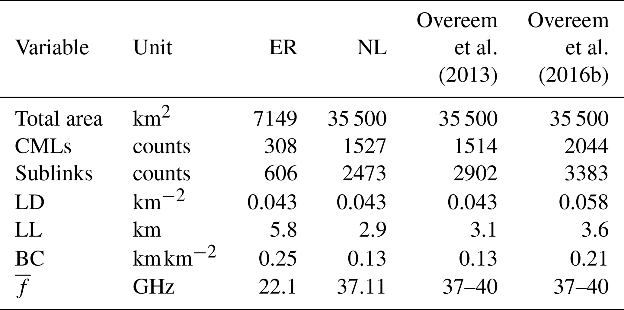
Since the RAINLINK original settings depend on the network characteristics, we compared the Emilia-Romagna network (ER) with one from the Netherlands (NL), which is included in the RAINLINK software package as a test sample (Overeem et al., 2016a), and with other datasets for which the algorithm was employed (Overeem et al., 2013, 2016b). The datasets' properties are summarized and compared in Table 1. ER has a comparable link density and higher average link length, resulting in a higher bulk coverage with respect to the NL network. The province of Bologna hosts more than half of the links (195 against 113) and thus has a higher LD.
2.1.2 Transmitting power levels
CMLs are usually equipped with automatic transmit power control (ATPC) devices which modulate the transmit power to guarantee a constant power level at the receiving end of the link, cancelling minor fluctuations in the total attenuation along the path. ATPC works at a higher frequency than 15 min and in a power window spanning 0 to +6 dB. With ATPC active, attenuation measurements should, therefore, be performed, subtracting receiving from transmitting powers, and are not possible from receiving powers only (Overeem et al., 2016a). The CMLs analysed in this work are equipped with ATPC, but unfortunately we do not have access to the transmitting powers, due to confidentiality restrictions. Luckily, provider engineers gave us instead some ATPC data – specifically, the maximum modulation offsets (in dB) that were applied during each time interval – through which we are able to correct the receiving power levels, compensating for the power modulation effects and simulating CML data with constant transmitting powers, allowing RAINLINK to estimate attenuations from receiving powers only. The correction intervenes only on minimum received powers (Pmin), which are no doubt affected by the ATPC: they are manually lowered by the maximum ATPC modulation applied within the respective 15 min time window. Maximum receiving powers (Pmax) are in contrast left untouched as the ATPC working frequency and the 15 min sampling frequency do not coincide and there was no way to infer a reasonable compensation. This could result in a broader gap between Pmin and Pmax.
2.2 Reference rain rate fields
2.2.1 Rain gauges
Rain gauge hourly and 15 min data are provided by Arpae RIRER (regional hydrometeorological network), established in 2001 by bringing together existing hydrological and meteorological station networks and managed at the time by various public bodies and local authorities. The network of the whole region is composed of 285 stations, equipped with tipping-bucket rain gauges: 110 of them are divided between the Bologna (54) and Parma (56) provinces. Rain gauges have different sampling intervals (from 10 to 60 min); they undergo a process of homogenization and quality control and are released as an hourly point-like product.
2.2.2 ERG5 rainfall analysis
The ERG5 gridded meteorological dataset has been developed by Arpae-SIMC, to support agricultural activities in the region of Emilia-Romagna. ERG5 data have been operationally produced since 2001, interpolating the hourly station measurements of the main meteorological variables (air temperature, relative humidity, precipitation, wind, solar irradiance) onto a 5 km×5 km grid covering the Emilia-Romagna region. The interpolation method used for hourly precipitation consists of a Shepard (1968) modified scheme using topographic distances instead of Cartesian distances. This allows the interpolation to take into account the influence of topography on precipitation, by making locations separated by orographic obstacles more distant than they would be if Cartesian distances were used (Antolini et al., 2016). Data are stored and distributed freely in the form of GRIB2 files, which were imported in an R environment thanks to the rNOMADS package (Bowman and Lees, 2015). Among all the variables included in ERG5, we consider here only the hourly accumulated precipitation. Its input is based on the same RIRER network described in the previous section, no longer limited to the two areas of study but extended to the whole region. Some discrepancies are therefore expected between the two products, mainly near the borders and in areas where the distribution of the instruments is less uniform.
2.2.3 Radars
The radar dataset is based on hourly precipitation estimates obtained from the composite of the regional radar network managed by Arpae-SIMC. The regional network is composed of two C-band systems, located in San Pietro Capofiume and in Gattatico (easternmost and westernmost red crosses in Fig. 1, respectively). For each instrument the equivalent radar reflectivity factor close to the ground is extracted and interpolated from polar coordinates to a 256×256 Cartesian grid of 1 km×1 km resolution and then merged to obtain a composite of both radars.
Raw radar images are affected by various non-meteorological echoes that are removed before computing the quantitative precipitation estimation (QPE). The current scheme used at Arpae-SIMC during operational service includes many steps: the ground clutter is removed at first statically through the map of signal-free elevations recorded in dry conditions and then dynamically by combining a beam trajectory simulation at the current atmospheric state (as measured by radio soundings) with a digital elevation model (Fornasiero et al., 2006). The beam-blocking reduction and correction is performed based on a geometric optic approach (Bech et al., 2003), while anomalous propagation is detected after the analysis of the echo coherence in the vertical direction (Alberoni et al., 2001). The final conversion between reflectivity and rainfall rate is performed on the corrected dataset using the classic relationship Z=aRb, with a=200 and b=1.6.
Rain rates are obtained every 5 min, and hourly total rain amount is computed by an advection algorithm which takes into account the movement of the precipitating systems. The algorithm is based on the computation of maximum cross-correlation between consecutive maps, leading to the estimate of the displacement vector for each precipitating system. The rainfall field is then reconstructed every minute between the observations and cumulated over each hour. Finally, radar QPE is adjusted with rain gauge data, via the spatial analysis of the ratio G∕R between rain gauge rainfall rates (G) and radar rainfall rates (R) over the station locations. The spatial analysis is obtained as the weighted mean of the G∕R values, where the weight is a function of both the distance of the grid point from the station and the mean spacing between five observations (Koistinen and Puhakka, 1981; Amorati et al., 2012). In this work we will compare the CML product with both adjusted and unadjusted radar QPEs.
The process chain which takes CML signals and returns rainfall maps is governed by the open-source RAINLINK algorithm (Overeem et al., 2016a) published on GitHub (https://github.com/overeem11/RAINLINK, last access: 25 October 2020) as an R package. We used the 1.14 version of the RAINLINK algorithm, available online from July 2019, and we added some minor modifications and optimizations (forked version available at https://github.com/giacom0rovers1/RAINLINK, last access: 25 October 2020).
3.1 CML rain retrieval algorithm
The algorithm works for both instantaneous power measurements and [Pmin,Pmax] pairs; for the present work we use the latter, at 15 min intervals. The algorithm treats Pmin and Pmax separately (we will then use Pi to refer to both alternatively). Two separate rain estimates Rmin and Rmax will thus be obtained. The retrieval process is summarized below, while we show more details of the data filtering in the Supplement.
-
Preprocessing. The raw input goes through three consistency checks concerning data formatting and labelling. Any multiple observations for the same “LinkID” and “DateTime” are discarded; each LinkID is verified to maintain the same metadata throughout the whole dataset (“Frequency”, “PathLength”, and antenna coordinates), and rows with “NA” (not available) values in any of the columns except for “Polarization” (which is assumed to be vertical if not indicated) are discarded as well.
-
Wet–dry classification. The samples are classified into wet and dry periods by assuming that rainfall is correlated in space, through the so-called nearby links approach (NLA), which works as follows. For each link, a time interval with a decrease in the received power is labelled as wet if at least half of the links in the vicinity (within a 15 km radius) experience a comparable reduction, i.e. if the medians of the attenuation and the specific attenuation of the nearby links are below −1.4 dB and −0.7 dB km−1, respectively. This is the second most computationally time-consuming step of the algorithm.
-
Baseline determination. A 24 h moving-window median of the quantity over the dry time intervals defines a reference level Pref (baseline). This is the computationally time-consuming operation of the algorithm.
-
Outlier filter and power correction. Outliers due to malfunctioning links can be removed again by assuming that rainfall is correlated in space. The filter discards a time interval of a link for which the cumulative difference between its specific attenuation and that of the surrounding links over the previous 24 h (including the current time interval) becomes lower than the outlier filter threshold, which is fixed at −32.5 dB km−1 h. After removing the outliers, the classification information is used to clean the receiving powers of the noise over the dry periods. The corrected powers will be equal to Pref in dry periods and Pi in wet ones.
-
Rain rate retrieval. Attenuation Ai is computed as . A fixed quantity Aa=2.3 dB is subtracted from the attenuation Ai in order to take into account the wet-antenna effect, which is independent of path length and is also assumed independent of frequency and rain intensity. If , then the specific attenuation ki (dB km−1) is calculated as ; otherwise 0 is returned. Path-averaged mean rain intensity Ri (mm h−1) is finally calculated using the k–R relationship Ri=a(ki)b, where the coefficients a and b are from Leinse (2007) and Leijnse et al. (2010) for vertical and horizontal polarization, respectively.
-
Path-averaged rainfall depth. To obtain a single-path- averaged rain depth, Ri is combined through a weighted mean: . The factor transforms rain rates into 15 min rain depths. The weight α varies between 0 (estimate derived from Pmax only) and 1 (estimate derived from Pmin only); we adopted the default value (α=0.33). We specify that, unlike Overeem et al. (2016a), we chose to keep the subscripts related to the original receiving powers; thus in our notation the rain rate Rmin is higher than Rmax because it is obtained from the most attenuated signal Pmin.
-
Interpolation. CML-path-averaged precipitation estimates are assigned to the midpoints of the links like point measurements (“virtual rain gauges”). Interpolation of the point-like measurements is performed at an hourly scale with ordinary kriging on a spherical semivariogram on the ERG5 grid. Sill and range parameters are estimated from the available rain gauge stations of 3 consecutive years. The nugget parameter is set as 1∕10 of the sill, as in Overeem et al. (2016a). The interpolated field is truncated if it becomes smaller than 0.05 mm, which is half of the minimum detectable rain from a rain gauge.
3.2 Preliminary discussion about the RAINLINK set-up for Northern Italy
The implementation of RAINLINK in Emilia-Romagna required some technical and conceptual considerations, based on the differences and similarities between the local and Dutch climatology, orography, and CML network features. We will describe them below:
-
The CMLs' operational frequency in our dataset spans 5.0 to 45.0 GHz. The default frequency allowance window of the RAINLINK algorithm is 12.5–40.5 GHz instead. We decided to extend it to 10.0–45.0 GHz but no further, so five CMLs belonging to the 5 to 10 GHz interval were left out. We then removed 10 other links, which had higher frequencies but whose sensitivities were below 0.1 dB mm−1 (see Supplement for more details). This was done to avoid contamination from coarse, low-sensitivity signals.
-
The average link density (0.043 km km−2) is the same as the one of the network used for the original set-up of the algorithm (see Table 1).
-
Spherical variogram parameters (see Sect. 3.1, point 7, “Interpolation”) were calculated for 3 years from a pool of validated rain gauges from the entire region. The range and sill are 36.12 km and 1.12 mm2, respectively. These values very much resemble the median for May and June of the outputs of the “ClimVarParam” subfunction of Overeem et al. (2016a), which approximates 30 years of Dutch climate (van de Beek et al., 2012). Accordingly, it is expected that both the network structure and the rainfall spatial patterns are similar between the Italian and Dutch sites. This assumption drives the choice for the correct value of the NLA radius of the wet–dry classification algorithm.
-
The differences to the Netherlands regarding orography are more relevant (see Sect. 2). We expect that rainfall patterns could deviate from the average behaviours described by the variograms when interacting with the complex orography of the hilly part of the region. However, we do not have enough data to calibrate the NLA radius at a small scale or considering geographical subsamples. Moreover, a shorter NLA radius could theoretically improve the consistency with the expected decorrelation length, but, given the network in the hilly region mostly consists of medium to long links, candidates which would fall inside the NLA radius could be too few to ensure a statistical significance of the samples. Thus, we left its value unaltered at 15 km, but we expect that some issues could possibly arise in the areas characterized by the most heterogeneous terrain.
-
The default k–R relationship from Overeem et al. (2016a) is also maintained as is, since Northern Italy and the Netherlands share a similar climate: the average drop size distribution (DSD) differences between the two countries are expected to be negligible (Caracciolo et al., 2006) and certainly lower than the expected variations in DSD along the link paths and during the 15 min time intervals (Tokay et al., 2017).
All the other algorithm's parameters were not specifically calibrated. The reasons behind this out-of-the-box approach are numerous:
-
As suggested by its authors (Overeem et al., 2016a), a solid calibration of the RAINLINK retrieval algorithm should be implemented exploiting numerous instruments along the link paths and organizing dedicated measurement campaigns, which was not feasible for us.
-
The overall temporal span should also allow the dataset to be split into two non-overlapping datasets for calibration and validation, but the total wet hours available to us was not enough to grant statistical significance to both subsets.
-
The gauge-adjusted radar product (which is commonly exploited in most CML studies) is not the one currently selected by the regional weather agency Arpae-SIMC as their quantitative reference, a choice that went in favour of the interpolated rain gauge product ERG5 (see Sect. 2.2.2). The spatial and temporal resolution of ERG5, however, is too low to perform an effective calibration.
Therefore we analysed some CML–rain gauge pairs only where the gauges were already in the vicinity of the links (Sect. 4.1), while we validated the rest of the dataset against the reference only through its interpolated product (Sect. 4.2.1 and 4.2.3).
We consider RAINLINK's ability to function as a stand-alone system – while other approaches rely on gauges or radars for wet–dry classification – as one of its key features. However, since RAINLINK does not include any standardized algorithm or procedure for calibration, performing it would lead to a huge increase in the set-up efforts, which would make other algorithms (where adaptation to local characteristics is naturally present, e.g. neural networks) much more competitive.
3.3 Error metrics
In the present work, we selected two sets of classical skill indicators, broadly used in the validation community (Nurmi, 2003): the first one is to assess the capability of the product to detect rainfall occurrence (categorical indicators) and the second one is to evaluate the skill in correctly estimating the quantitative precipitation rate (continuous indicators). The first set is computed after a definition of a confusion matrix by counting the number of samples where both the estimate and the observation agree on classifying wet (hit, H), or dry (correct negative, CN) samples, and where there are misses (M, observed wet and estimated dry) or false alarms (F, observed dry and estimated wet). Namely, the probability of detection (POD), false alarm ratio (FAR), multiplicative bias (MB), and equitable threat score (ETS) are defined, respectively, as
where Hrnd represents the number of hits obtained by chance.
Given ei and oi as estimated and observed values, respectively, continuous indicators are the normalized mean error (ME) and the normalized mean absolute error (MAE), defined as
plus the coefficient of variation (CV), defined as the root mean square error divided by the mean of the observed values , and Pearson's correlation coefficient (CC), defined as the covariance of observed oi and estimated values ei divided by the product of the two standard deviations (Nurmi, 2003; Overeem et al., 2016b).
Both the interpolated CMLs and the reference field have a large number of very low positive values (below 0.1 mm h−1) that do not have any physical relevance but which are potentially very influential in normalized error metrics. Thus we have set a wet–dry threshold equal to the minimum rain quantity detected by the tipping-bucket rain gauge, i.e. 0.1 mm h−1, for both estimate and reference. Categorical indicators are calculated with respect to this threshold for the whole dataset, while all the continuous indicators are computed only for the product–reference pairs where both values exceed the threshold (i.e. wet–wet). ME, MAE, and CV are normalized with the averaged reference rain depth.
We carried out the validation of the CML product at three different levels. First, we compared single-link estimates with the measurements of a nearby rain gauge, at the shortest temporal scale available (15 min), to discuss success and failure cases, trying to understand the latter. Secondly, we compared the interpolated 5 km×5 km CML hourly rainfall maps vs. the ERG5 product at a grid box scale, also analysing three case studies. In the third step, the map comparison is carried out at a basin scale including even the other precipitation products available at Arpae-SIMC.
4.1 Single-link verification
We have selected links in rural areas and different terrains with an active rain gauge close to the link: the distance between link and rain gauge, reported in Fig. 2, is always below 3 km (significantly lower than the correlation distance of precipitation in Italy; Puca et al., 2014) and always lower than the length of the link itself. In general, no dependence of the link performance on the distance from the rain gauge is found. Selected links had to be active for the whole analysed period. In many cases more than one link was selected for one rain gauge. Temporal sampling is kept at the highest frequency, which is a measurement every 15 min for both the CML and the rain gauges. A total of 12 rain gauges and 26 CMLs were chosen, 14 of which are in the northern part of the domain and the other 12 on the hilly region at elevations between 193 and 960 m a.s.l.
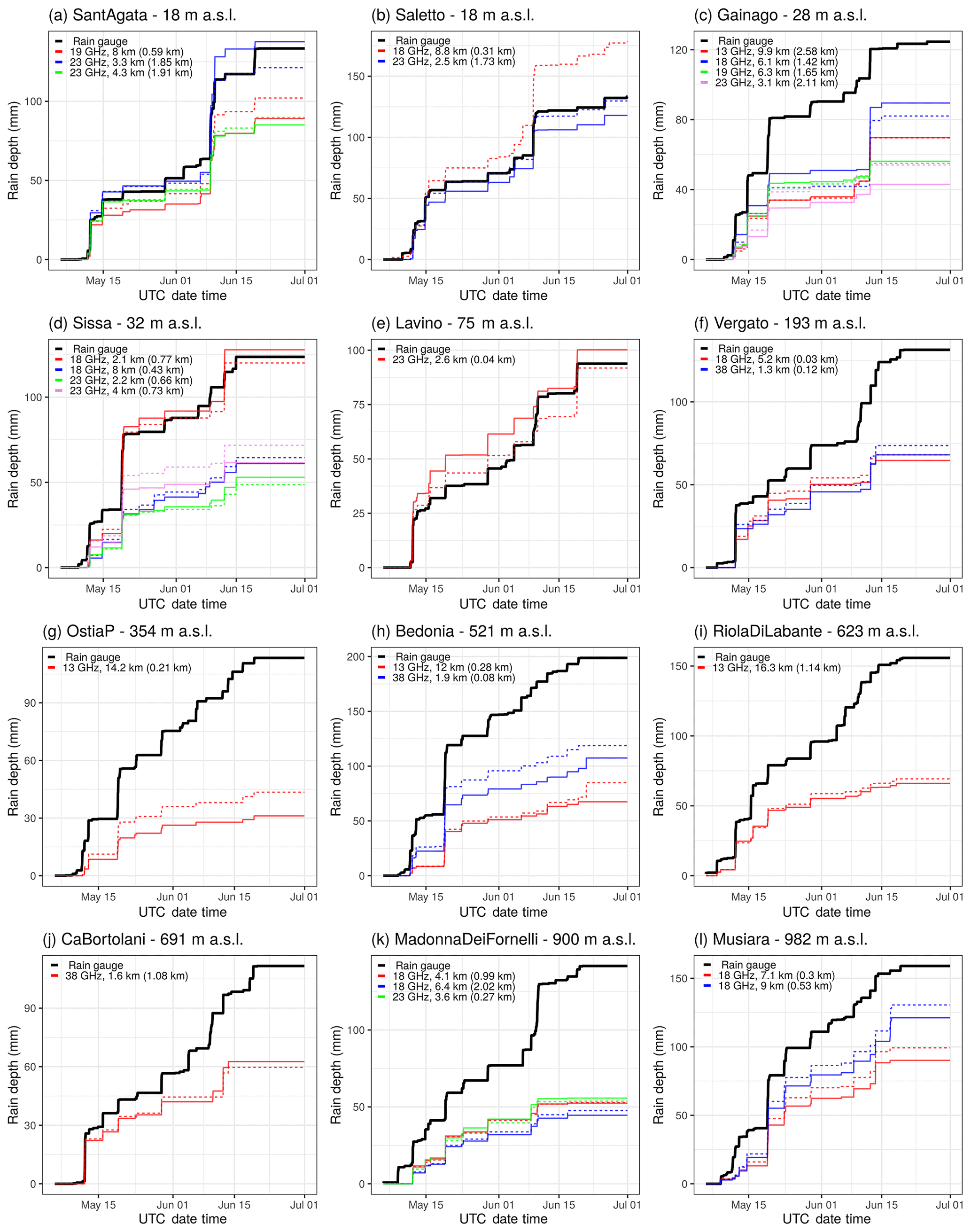
Figure 2Accumulated rain depths over the entire period for the 26 CMLs selected for the single-link analysis. Each panel is named with the corresponding rain gauge, whose accumulated rain depth is shown by the thick black line. Solid and dashed lines represent the two directions (if both active) for every CML (distinguished by colour). Link length and link–rain gauge distance, in brackets, are also reported.
The rain depths of the 26 CMLs are reported in Fig. 2 for the whole study period, grouped according to the closest rain gauge and ranked by its altitude. A large variability is found (ranging from near-perfect agreement to discrepancy of a factor of 2 or 3 in the worst cases). Of the 26 links' CCs, 75 % are between 0.5 and 0.88, with an overall median value of 0.68, proving an acceptable overall skill. We relate this variability to the heterogeneity of CML sensitivity, the small scale of the meteorological events (see Supplement), and different site exposures and elevations. In most cases, CMLs underestimate the rain gauge values: the links located in the lowlands (Fig. 2a, b, d, and e) show a better correspondence than those in the hilly regions, where underestimation is more significant.
In some cases (Fig. 2f, k, and l) the discrepancies between CMLs close to the same rain gauge (but different in location, frequency, and length) are much lower than the CML–rain gauge differences: all these CMLs are in good mutual agreement and share the same classification issues, resulting in a systematic underestimation which therefore seems to be caused by the algorithm set-up. In other cases (Fig. 2b, d, and g) some links clearly outperform other members of the same group. This second kind of discrepancy is more likely related to real differences, like inhomogeneous rainy structures which crossed the link paths or different hardware set-ups, while there is no evidence of a correlation with frequency or path length. The difference between the two directions of the same link is generally below 10 %, except for the Ostia Parmense site (see Fig. 2g).
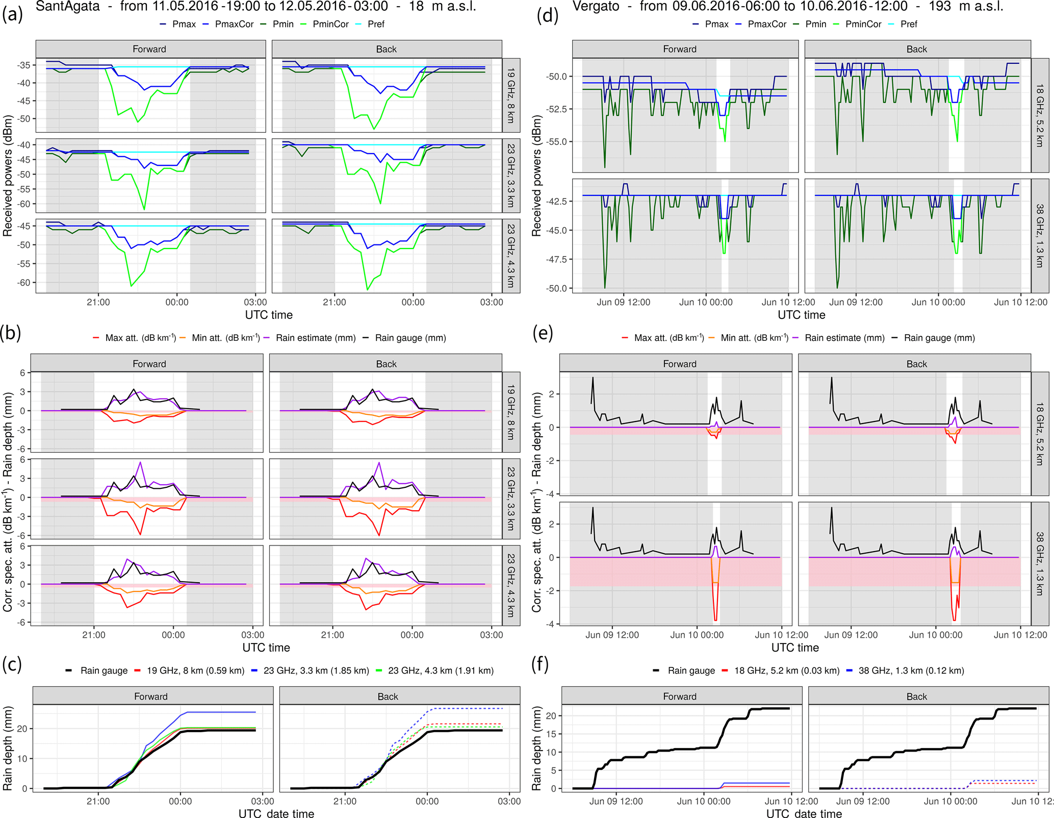
Figure 3Single-link analysis for Sant'Agata (from 11 May 19:00 UTC to 12 May 03:00 UTC) and Vergato (from 9 June 06:00 UTC to 10 June 12:00 UTC): (a) and (d) show the received signals (Pmax, dark blue; , light blue; Pmin, dark green; , light green; Pref, cyan); (b) and (e) show maximum attenuation (red), minimum attenuation (orange), estimated rain rate (purple), and gauge measurements (black); in (c) and (f) the cumulated rain gauge rain rate (black) is plotted with the link estimates. Grey vertical bands correspond to intervals labelled as dry by the NLA classification; pink horizontal bands correspond to the threshold in decibels per kilometre of the wet-antenna correction of 2.3 dB. The y-axis ranges are specific for each CML as received powers differ between different path lengths.
To gain a deeper understanding of better and worse performance of the single links, we performed a more detailed analysis of case studies at the rain-event scale (Fig. 3). We show a case when the link retrievals accurately match the measurements of the nearby rain gauge and a case with markedly low performance. In Fig. 3, graph panels are organized in columns by CML and in rows by sublink. In panels a and d are shown all the signals managed by the algorithm: the reference power Pref, the raw received powers Pmin and Pmax, and the filtered received powers and . In panels b and e rain gauge measurements are compared with CML estimates, and the minimum and maximum attenuation signals are also plotted (Amax and Amin, respectively). The grey background indicates when the classification detects a dry period. The pink background indicates the band inside which attenuation is considered to be caused by a wet antenna (Aa parameter) and is discarded for rain retrieval. Panels c and f show the cumulated rainfall depths in the same time frame.
4.1.1 Best-case example
Between 11 and 12 May 2016 an extensive convective system covered the Bologna Province area almost entirely, with a maximum rain rate of 23 mm h−1 and widespread precipitation. For this case, the NLA classification on the three links near Sant'Agata (Bologna Province, 18 m a.s.l.) works properly: in Fig. 3b most of the measured rain is on the white background. In Fig. 3a, after the attenuation event, the noisy signal is correctly filtered, and a very small amount of rain (just above the gauge threshold) is neglected. The agreement is qualitatively very high between each pair of sublinks and good among the different links, in terms of specific attenuations and retrieved quantities (see Fig. 3b). Quantitative retrievals give some overestimation for one of the CMLs, whose effect is evident on the accumulation plot (Fig. 3c) where the total rain depths are compared. During the 2 months, the Sant'Agata links are generally in good agreement with the nearby rain gauge, with CC values ranging between 0.66 and 0.88 and CV values between 0.47 and 0.96.
4.1.2 Worst-case example
Between 8 and 10 June 2016 an event hit the Vergato site (Bologna Province, 193 m a.s.l.). It was characterized by intense rainfall peaks (rain rate up to 14.6 mm h−1) and iterated moderate scattered precipitation. Many wet intervals are missed due to wet–dry misclassification (Fig. 3e), leading to a 20 mm loss in the rain accumulation (Fig. 3f). The POD over the entire period for these two links is between 0.22 and 0.29.
In the case when the NLA classification correctly identifies some rain occurrence, there is still a general quantitative underestimation. It could be seen that half of the signal is hidden from the wet-antenna attenuation threshold. The continuous scores for the wet–wet sample over the entire period show a good correlation with gauges but are poor in statistical relevance because of the high number of misses. They nevertheless confirm the tendency to underestimate, by around 40 % ().
4.2 Gridded product verification
The verification of the RAINLINK gridded product (1 h cumulated on the 5 km×5 km grid) with respect to the ERG5 product is first performed at the highest available resolution (grid box by grid box), since the two products intentionally share the same interpolation grid (see Fig. 4). Secondly, the comparison is carried out at the basin scale by matching spatially averaged time series over areas of different size, in parallel with other operational precipitation products available at Arpae-SIMC.
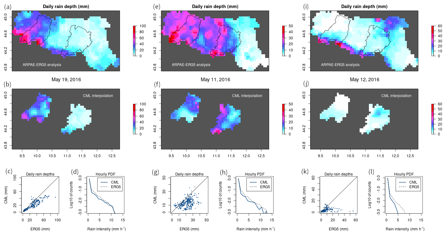
Figure 4Analysis of three 1 d case studies (19 May, a–d; 11 May, e–h; 12 May, i–l): (a, e, and i) daily cumulated ERG5 precipitation; (b, f, and j) daily cumulated RAINLINK precipitation; (c, g, and k) scatter plot between the two daily precipitation values; (d, h, and l) PDF of hourly rain rates.
4.2.1 Highest-resolution matching
Figure 5 shows a density scatter plot for the whole dataset over the entire period. CML estimates from RAINLINK in Northern Italy over uneven ground have an overall underestimating performance of −26 % on the accumulated rain over the 2 months. The CV is 0.78 and R2 (the square of Pearson's correlation coefficient CC) is 0.46, based on a sample of 10 672 total wet hours. To make the comparison with past works easier, we computed continuous indicators with the filter set as reference >0.1 mm and with no filtering at all. Results with the first setting yield worse indicators, increasing the ME to −0.41 and the CV to 0.95, with a second digit increase for R2, around 0.5. The no-filter run shows values of and R2=0.53, which are aligned with our most filtered results, while CV=4.6 is greatly affected by very small rain rates. These results are in agreement with similar studies (Overeem et al., 2013, 2016b) despite the differences in the products involved; comparisons between our results, with both filters, and the ones presented in the mentioned works are shown in Table 2.
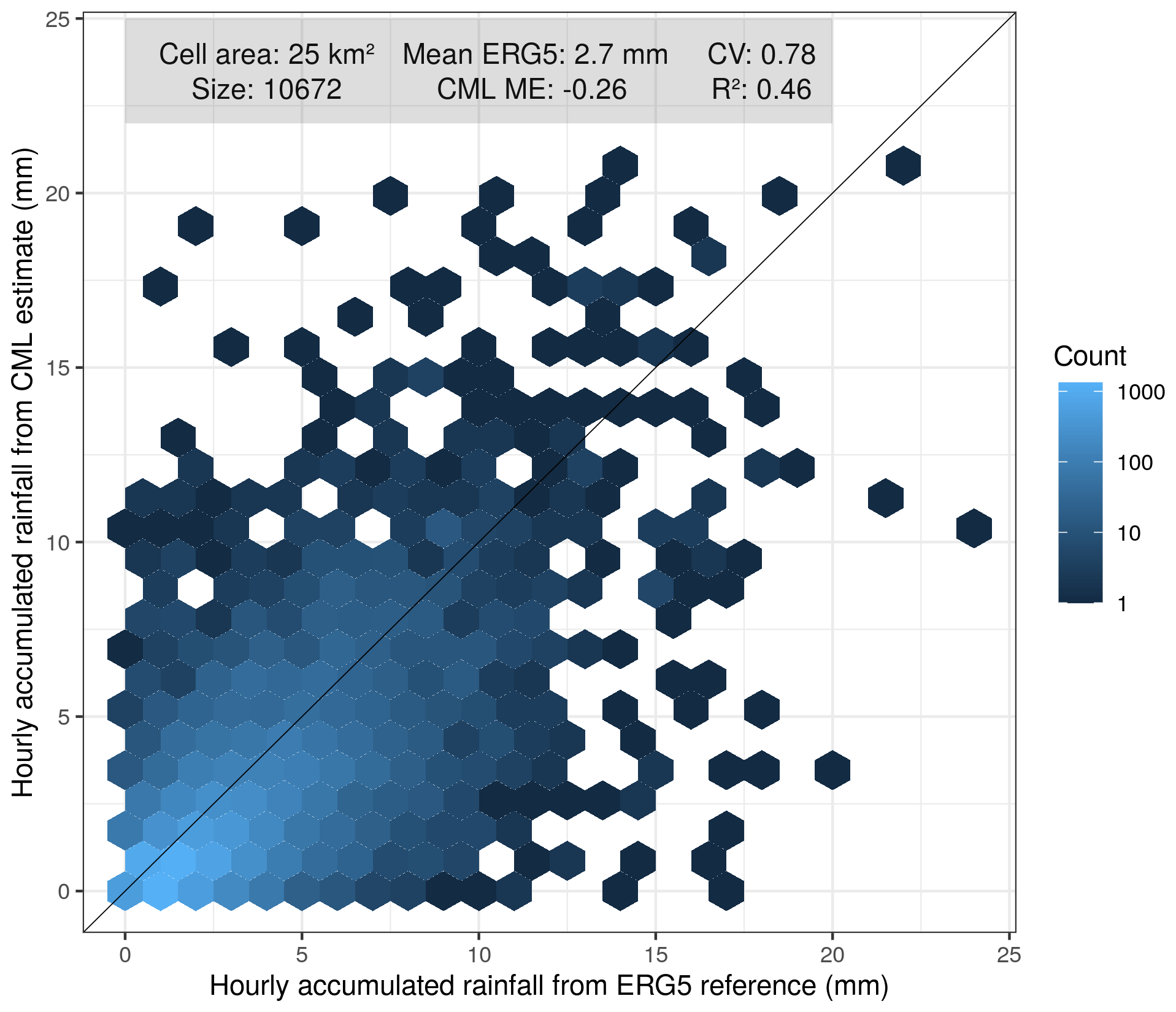
Figure 5Hourly validation of link rainfall maps against ERG5 rainfall maps at the grid box scale (highest resolution). Only the rainfall depths in which both CMLs and ERG5 measured >0.1 mm were used. The black line is the y=x line.
Table 2Comparison with previous studies. Ref is the reference rain rate; Pr is the product.

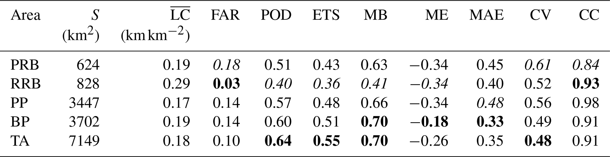
Table 3Statistical indicators for each considered area, considering the highest-resolution information (grid box scale), shown in ascending order of . Continuous indicators are normalized and fractional. Values in bold (italics) are the best (worst) values in the column.
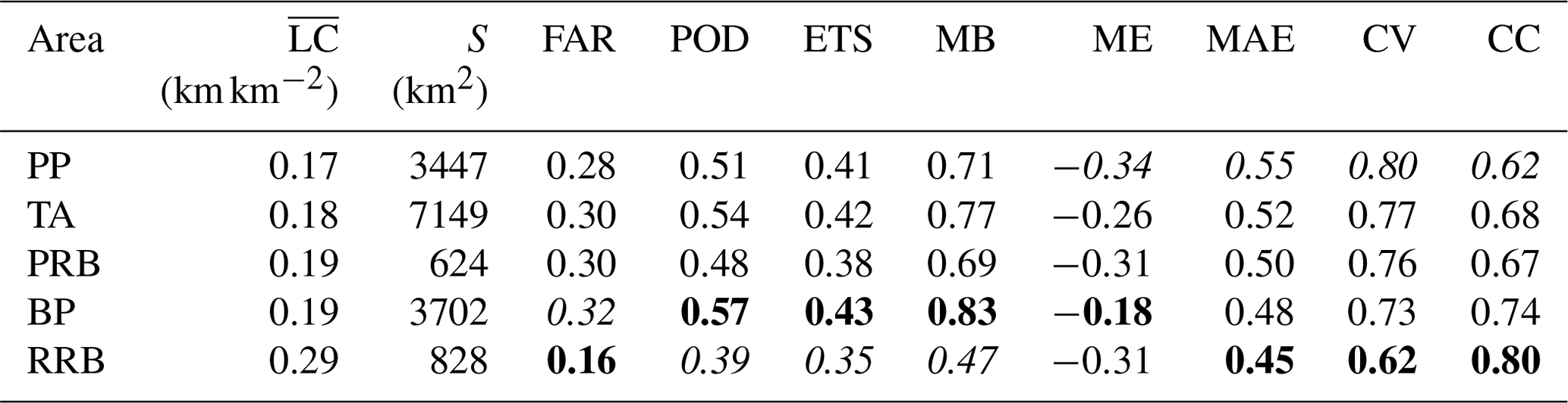
The performance of the rain detection capabilities with respect to the 0.1 mm threshold is evaluated by the set of categorical scores defined in Sect. 3.3. Quantitative continuous indicators from now on are computed only for the grid boxes where both CML and ERG5 reported more than 0.1 mm at the same time. Categorical and continuous indicators are evaluated for five areas, with a different extension (S) and average link coverage (). They are reported in Table 3, ranked according to the value: Parma Province (PP), total area (TA), Parma Basin (PRB), Bologna Province (BP), and Reno Basin (RRB). The total area and the two provinces do not have any specific hydrological meaning but may resemble larger river basins with heterogeneous terrain (see Fig. 1). All normalized indicators are relative to the average reference (ERG5) rain rate. Numbers in bold (italics) are the best (worst) value in the column.
We found ETS values ranging from 0.38 to 0.43, which are comparable with the ones obtained from satellite observations (Puca et al., 2014; Feidas et al., 2018) in similar regions. For four out of five areas (excluding RRB for now) the RAINLINK product underestimates the rain occurrence (MB<1), with a relatively low value of POD (0.48 to 0.57). The FAR is also rather small, (0.28 to 0.32), resulting in low ETS values (0.38 to 0.43). The mean error confirms the underestimation of rain amount (ME between −0.18 and −0.34); the CV ranges between 0.73 and 0.80 and CC between 0.62 and 0.74. For comparison, Petracca et al. (2018) analysed over Italy the instantaneous estimate of the Global Precipitation Measurement Dual-frequency Precipitation Radar (GPM DPR), considered the most reliable and accurate instrument to measure precipitation from space. Over a footprint of a size comparable to the one used in this paper, the best value of CC is 0.57, while the CV was between 1 and 2. Other validation studies of GPM DPR products in the alpine region (Speirs et al., 2017) obtained a relatively good POD (up to 0.78), FAR (below 0.08), and CC (up to 0.63) over flat terrain, with a dramatic drop of the skill indicators when areas with complex topography were considered.
The averages over the Reno Basin stand out for all the indicators, either positively or negatively; therefore they need a separate description. As highlighted in Table 3 in bold and italics fonts, RRB has half the FAR of the other samples (0.16), a CV almost 10 points lower (0.62), and a CC nearly 15 points better (0.8, which is unexpectedly high), with the mean errors aligned to the other samples. The higher accuracy in the estimates is reached at the expense of POD, ETS, and MB: around 50 % of the rainfall duration is lost in this area. The main peculiarity of the RRB area is the high , which is 50 % higher than in the rest of the regions.
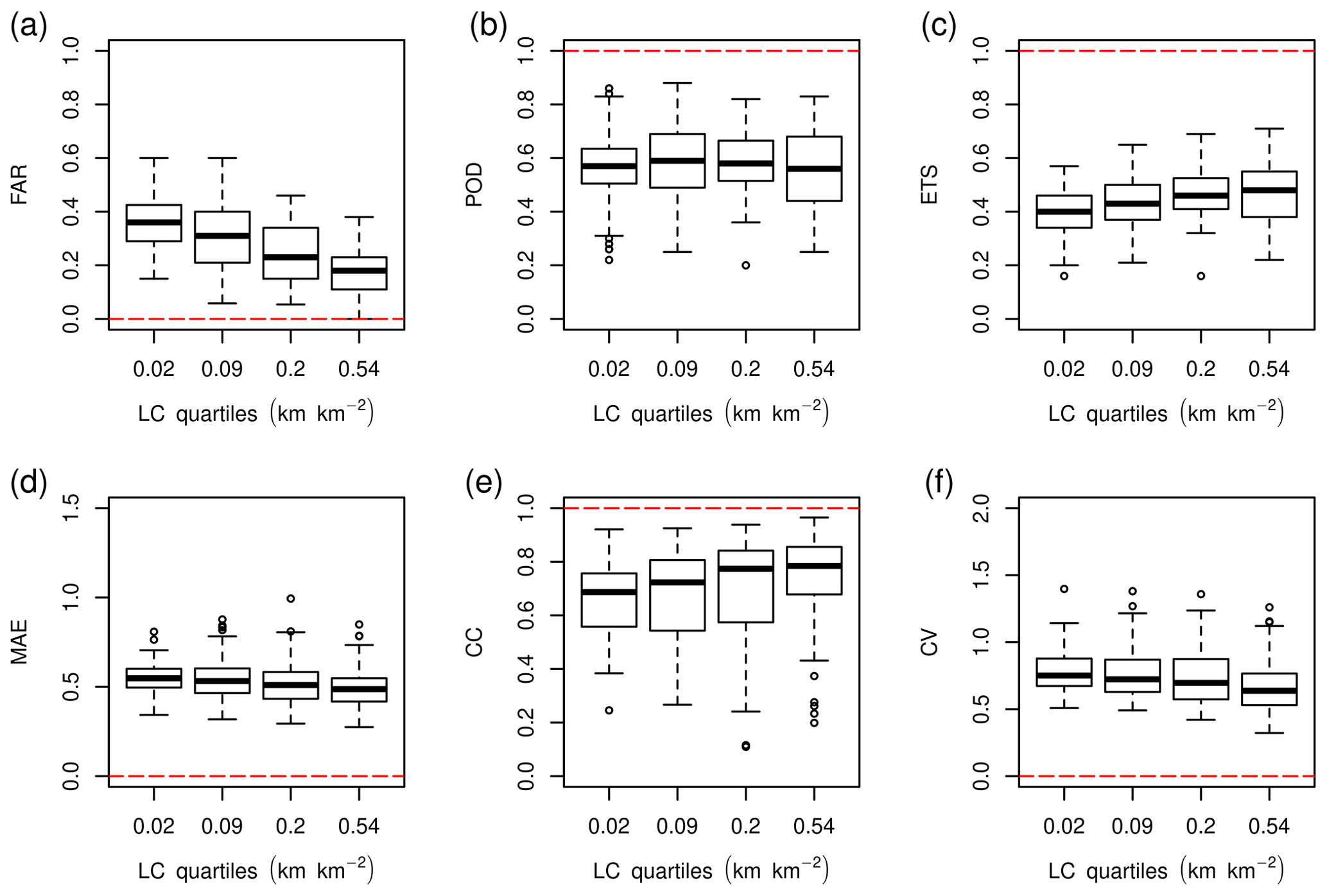
Figure 6Distributions of four statistical indicators computed for every grid box and grouped in box plots by quartiles of the link coverage LC (labelled by the quartiles' centres). Dashed red lines are the optimal values for each score.
The marked improvement of continuous indicators for RRB suggests that the quantitative matching between the estimate and reference could be positively related to . Thus, we further investigate its effect on scores by grouping each grid box by LC quartiles, regardless of the actual geographical location, and we reported the results in Fig. 6. Five out of six indicators improve as LC increases (FAR, MAE, ETS, CC, and CV), among which the most striking is the FAR, while POD remains mostly unchanged, allowing the ETS improvement.
4.2.2 Case studies
To assess the performance of RAINLINK with respect to the structure of rainfall fields we focused the analysis on three 1 d long events with different characteristics, for which RAINLINK provided results of varying quality.
Table 4Rainfall characteristics and performance indicators for the three 1 d case studies.
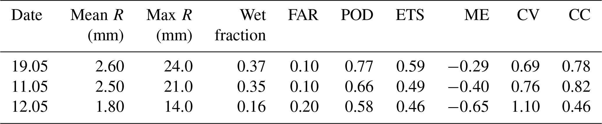
The best performance was achieved on 19 May (see Fig. 4a–d), when an intense event was characterized by a few convective episodes on the Apennines, in the Parma Province. Precipitation peaks were around 90 mm d−1 (see Fig. 4c); maximum and mean hourly rain rates were about 24 and 2.6 mm h−1, respectively (see Table 4). A large area of widespread moderate precipitation over the Bologna Province (Fig. 4a) is also present. RAINLINK is able to localize precipitation local maxima (Fig. 4b), even if the precipitation occurred in areas where link coverage is relatively poor (see Fig. 1), also providing accuracy in the peaks' intensity. Estimated PDF closely matches the ERG5 curve, indicating that all rain rates are represented in the estimates (see Fig. 4d). However, underestimation is present at all ranges and more markedly at the highest rain rates. Numerical indicators confirm the goodness of the estimate, in terms of wet-area detection (ETS = 0.59) and relative error (CV = 0.69), while the fractional amount of rain lost by the estimate is low ().
The second case (11 May) shows a more patchy rainfall field (Fig. 4e), which resulted from a series of storms that occurred in the area during the day. Maximum and mean rates are lower with respect to the first case (Fig. 4g and h), as well as the wet fraction of overall samples (see Table 4). Some local peaks are correctly located (especially inside the Bologna Province), as shown in Fig. 4f, and some others, in Parma Province and particularly on the Apennines, are missing. In this case the underestimation is marked for all rain rates, resulting in a higher ME (−0.40) and lower POD (0.66).
A completely different scenario is represented by case three (12 May), when ERG5 measured light to moderate precipitation (see Fig. 4i), with maxima on the Apennines and a much lower fraction of wet samples. RAINLINK (Fig. 4j) is not able to estimate the highest rain rates or to locate the area with the highest intensity. Moreover, it finds a spurious peak in the northern area of the Bologna Province, which is not detected by ERG5. Here the fractional amount of rain loss is −65 %, the POD is low, and an increase in FAR is also to be remarked upon, indicating that underestimation again dominates throughout the whole range of rain rates (see Fig. 4k and l), but in the case of light rain, overestimation can also take place.
4.2.3 Areal averages matching
In this section, the matching between estimate and reference field is performed at basin (and province) scales, comparing hourly rain amounts averaged over areas of different sizes. The areas selected for this evaluation are the ones introduced in the previous section: two of them are chosen because of direct hydrological interest (RRB and PRB), while the other three (BP, PP, and TA) are selected to assess the impact of the increasing target area.
Table 5Values of the statistical indicators for the mean rain amounts over each considered area, shown in ascending order of surface area S. Values in bold (italics) are the best (worst) values in the column.
In Table 5 we present the categorical indicators calculated around the 0.1 mm h−1 threshold and the continuous indicators calculated on wet–wet occurrences only, for the five mentioned areas listed this time in order of increasing area size. In general, the best performance is found for the largest areas (BP and TA), while the smallest ones (PRB and RRB) show the worst values. The CML product underestimates precipitation occurrence (MB between 0.41 and 0.70) and amount (ME between −0.18 and −0.34) at all scales. Due to the areal averaging, the CC is markedly higher than the high-resolution values reported in Table 3. The characteristic behaviour of RRB (lowest FAR and POD, highest CC) also applies in this case.

Figure 7Scores of the areal-averaged rainfall amounts grouped per sensor and plotted against basin area. Linear fits are highlighted with dashed lines. The CML scores are also indicated numerically in Table 5.
The same areal-averaged statistical indicators have also been computed for all the operational products available at Arpae-SIMC for routine use and described in Sect. 2.2, reported on an hourly scale and compared with the ERG5 product. We show in Fig. 7 the values of the statistical indicators as a function of the target area.
The rain gauge product, obtained by averaging the measurements of the rain gauges in the area, performs similarly to its interpolated version ERG5, as expected, and diverges only for small areas, where the impact of a single sensor in disagreement with neighbours is the highest.
The radar product shows, in this metric, almost the same performance both with and without the gauge adjustment1. Both have very good detection capabilities (POD is almost 1) but high rates of false alarms (FAR around 0.5) and marked quantitative discrepancies (MAE around 0.9; CV between 0.75 and 2).
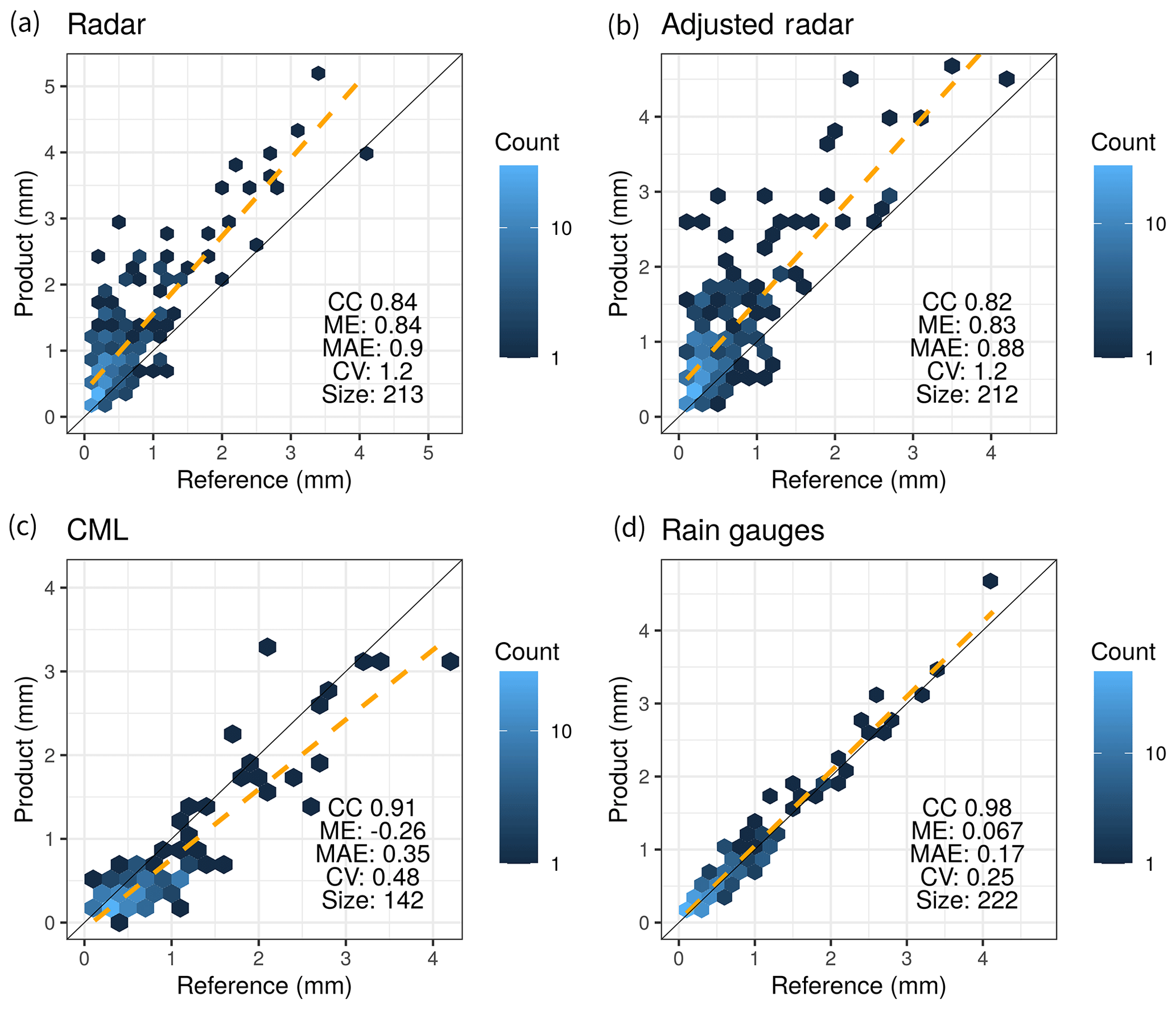
Figure 8Comparison of hourly areal-averaged rainfall depths from the four products against the ERG5 reference. The total area (TA) wet–wet hours are considered.
The CML product outperforms both radar products in terms of CC, CV, MAE, and FAR, while it lacks in detection capability (CML POD between 0.4 and 0.6). Figure 8 shows that the overestimating and underestimating behaviours of radar and CML products, respectively, can be seen as complementary. For radars, the spread is more relevant than for CML, but it has to be remarked that the latter has a smaller sample size due to the already-mentioned low POD issues. It also has to be said that part of the radar's high FAR and overestimation could represent real rain from small precipitating structures, often observed between meteorological spring and summer in Italy (see Supplement), that are randomly missed by the rain gauges (and therefore by the ERG5 reference product as well).
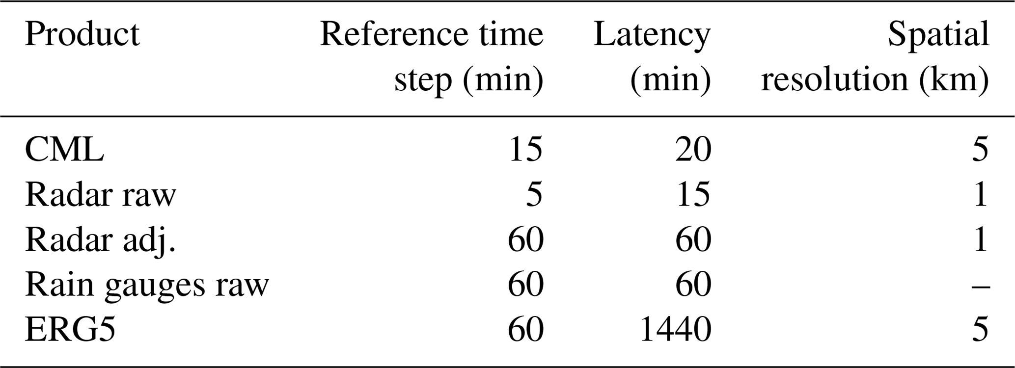
In Table 6 the latency and sampling characteristics of the four precipitation products we took for comparison are reported, along with the CML product. CML operational specifications refer to an implementation of the RAINLINK algorithm as part of a real-time service, tested in 2019 by MEEO S.r.l. within the RainBO project (LIFE15 CCA/IT/000035).
Table 6Latency and spatial and temporal sampling of the considered precipitation products.
The underestimating behaviour that emerged in the single-link-versus-gauge analysis (Sect. 4.1) seems to be largely imputable to a wrong wet–dry classification. Though we do not have a dataset large enough to support general statements, looking at Fig. 3d we could gain some insights about what goes wrong in two of the most problematic CMLs of our population, the Vergato ones.
Most of the rain which is sensed by the gauge falls in intervals that the NLA reports as “dry” (grey background). Pmin in fact clearly experiences some decrease, which is coupled to the missed rainfall, but Pmax does not. This behaviour of Pmax is not an issue in itself, as the NLA classification relies on Pmin only. It indicates, however, that there are power fluctuations which happen faster than 15 min; otherwise Pmax would have decreased too. Rapid fluctuations, in turn, suggest irregular, rapidly varying, or scattered precipitation patterns. These are actually elements that could affect the correct classification, since NLA relies on the spatial correlation of the rainfall field in a range of 15 km (see Sect. 3.2). Therefore, a Pmax signal which remains always near the baseline could be a precursor of local NLA issues. Classification errors are likely the best explanation for the low POD scores.
Given how we filtered the data (product >0.1 and reference >0.1), we need a source of error other than the misclassification to be responsible for the quantitative underestimation measured by the set of continuous indicators (see Sect. 3.3 for reference). We saw that half of the signal in the correctly classified interval (Fig. 3e, white background) remains under the wet-antenna attenuation threshold (pink horizontal band). We can presume that the antenna is actually dry, so the Aa threshold in this case is reasonably too high (as also noted by de Vos et al., 2019). However, a simple sensitivity test, carried out to assess the impact of a decrement in the Aa threshold on the single-link-versus-gauge scores, did not lead to any substantial improvement, especially if the new value was used to process the whole dataset. More information is provided in the Supplement.
Comparing the average performance of the interpolated product (Sect. 4.2) above the different subareas, particularly with respect to the RRB one, we can infer that higher mean coverage () leads to a more selective NLA classification, which reduces the FAR and POD. When grouping the single grid boxes based on their coverage (see Fig. 6), it seems however that the sensitivity to LC could explain only the improvement in FAR and not the sharp decline in POD, suggesting that LC was probably not the only variable at play in the Reno Basin. These results integrate the findings of Overeem et al. (2016b) that highlighted the positive impact of higher on the CV and CC at a lower spatial resolution. Other studies will be conducted in the future to gain more insights into these topics.
Looking at a daily scale (Sect. 4.2.2), the interpolated output of RAINLINK is undoubtedly able to resolve small-size, short-lived events and even provide quantitatively accurate estimates. In the case of widespread, moderate precipitation the overall rain pattern is still effectively represented, but some underestimation of the numerical values appears. When in the presence of light and intermittent rainfall, instead, we see the consequences of the issues emerged during the single-link analysis. The rainfall maps in the panels i and j of Fig. 4 reveal that the discontinuity of the link distribution across the borders of the considered areas could be another possible source of discrepancies. We give more insight about this issue examining the maps of the total rainfall accumulation in the Supplement.
Even knowing that the limitations we have just discussed are not negligible, we can still compare the interpolated CML product's performance with that of the traditional ones, to see whether some overall sensing skill is present or not. We used the areal-averaged hourly rainfall accumulations (see Sect. 4.2.3) to compare products with different spatial resolutions. The comparison between radar and CML is particularly interesting as they appear to be rather complementary data sources. The CML product in this set-up clearly lacks the detection capability (POD) of the radar. The CML retrieval process however, being based on electromagnetic attenuation instead of backscattering, does not share the radar's high sensitivity to the drop size distribution (Leijnse et al., 2008). This could make the CML a more robust sensor, in the sense that the same coefficients can be applied regardless the different types of rain (convective, stratiform, mixed), and the values of the continuous indicators seem to endorse that.
Alongside the considerations of the sensing skills, the time which will elapse from the acquisition of primary data (ideally, the occurrence of the event) to the actual delivery of the product ready for use is also valuable to a forecaster in an operational context. We referred to this as “latency”. It can be seen from Table 6 that the combination of short latency and high resolution provided by CMLs is unmatched by all the other products except the raw radar, which however lacks the required quantitative accuracy. It is left to the operators' preference, based on products' error structures, current meteorological conditions, and customer requirements, to make use of the most suitable product or of a combination of them. CMLs are valuably able to widen the range of available options.
An assessment of the rainfall retrieval capability of CML opportunistic sensors over complex terrain in Northern Italy is conducted at different spatial and temporal scales for 2 months of data. We implemented the open-source RAINLINK algorithm in a new area and context, where no regional CML studies had previously been performed. We evaluated its performance through a complete validation scheme which utilizes operational precipitation products as reference, at the same time also gauging the implementation efforts and identifying major strengths and weaknesses to facilitate the profitable use of CML products.
First, 26 CMLs are compared with the closest rain gauges at a 15 min scale. Overestimation and underestimation of rain amount are both present, though the latter appears dominant. A marked variability among different links does not prevent the achievement of a generally acceptable skill (CC from 0.50 to 0.88). The wet–dry classification approach (NLA, based on the spatial correlation of the rain) and the value of the wet-antenna correction (Aa) may produce some misses in both rainfall occurrence and amount, particularly in the case of small-scale or intermittent episodes. Finally, CMLs located at higher elevations generally show worse performance.
Interpolated products obtained from 308 links not only confirm that a non-negligible quantity of rain is missed (normalized mean error is −0.26; overall CC is 0.68; and overall CV is 0.78) but also show that the rain retrieval capability is suitable for operational application, especially if the product is integrated over large areas (CC rises to 0.92). Higher link densities increase the quality of the CML estimates at both grid box and basin scales, mostly in terms of a decreased FAR.
Performance at the daily scale shows enhanced skill in the case of heavy precipitation, even in the case of localized episodes. Problems arise instead during light to moderate rainfall, when the limitations that emerged during the single-link analysis become evident. Negative impact on the overall results comes from areas with poor sensor coverage, especially near the borders of the studied areas, but it should be considered that reference rainfall fields can also be affected by shortcomings of the same nature.
Furthermore, when compared to other products currently available for real-time operational exploitation, the RAINLINK output shows similar or better abilities, especially if a low FAR is valued more than a high POD and if latency is also taken into account. The integration of a CML-based product into an operational weather service appears worthwhile, even in a plug-in implementation that omits specific local calibration.
CML data were provided by Vodafone Italia S.p.A.. via direct purchase from MEEO S.r.l. and are not publicly available. Gauge data from Emilia-Romagna are freely available at https://simc.arpae.it/dext3r/ (SI@SIMC@ARPAE, 2020). Radar reflectivities in near real time are freely available at https://dati.arpae.it/dataset/radar-meteo (SIMC, 2020), while derived rain products and ERG5 analyses are available upon request at Arpae-SIMC (https://dati.arpae.it/dataset/erg5-interpolazione-su-griglia-di-dati-meteo, Osservatorio Clima, 2020). The core algorithm is available open source at https://github.com/giacom0rovers1/RAINLINK; it was forked from Aart Overeem's original RAINLINK (Overeem et al, 2016a; https://doi.org/10.5281/zenodo.4153473, Roversi, 2020) on 26 August 2019 (version 1.14).
The supplement related to this article is available online at: https://doi.org/10.5194/amt-13-5779-2020-supplement.
GR adapted the RAINLINK code to Italian data, ran the analysis, plotted the data, and contributed to the interpretation of the results and to the writing of the manuscript. PPA and AF performed the reference data preprocessing and contributed to data analysis. FP contributed to the design of the validation strategy, to the interpretation of the results, and to the writing of the paper.
The authors declare that they have no conflict of interest.
The authors thank Stefania Pasetti and Marco Folegani of MEEO S.r.l. (http://www.meeo.it, last access: 25 October 2020) for their support and are grateful to Davide Vecchiato and Antonio Viaro of Vodafone Italia S.p.A. for their technical assistance with the data. We also thank Aart Overeem for having developed and released the open-source RAINLINK algorithm and for the kind feedback and support he provided for this research.
This research has been partially supported by the LIFE financial instrument of the European Commission (grant no. LIFE15 CCA/IT/000035).
This paper was edited by Gianfranco Vulpiani and reviewed by two anonymous referees.
Abdulrahman, A., Bin Abdulrahman, T., Bin Abdulrahim, S., and Kesavan, U.: Comparison of measured rain attenuation and ITU-R predictions on experimental microwave links in Malaysia, Int. J. Microw. Wirel. T., 3, 477–483, https://doi.org/10.1017/S1759078711000171, 2011. a
Alberoni, P. P., Andersson, T., Mezzasalma, P., Michelson, D. B., and Nanni, S.: Use of the vertical reflectivity profile for identification of anomalous propagation, Meteorol. Appl., 8, 257–266, https://doi.org/10.1017/S1350482701003012, 2001. a
Alberoni, P. P., Fornasiero, A., Roversi, G., Pasetti, S., Folegani, M., and Porcù, F.: Comparison between different QPE based on: Microwave Links, Radar adjusted and Gauges, in: 10th European Conference on Radar in Meteorology and Hydrology, KNMI, 1–6 July 2018, Ede, the Netherlands, 851–860, https://doi.org/10.18174/454537, 2018. a
Amorati, R., Alberoni, P., and Fornasiero, A.: Operational Bias Correction of Hourly Radar Precipitation Estimate using Rain Gauges, in: Proceedings of the Seventh Eropean Conference on Radar in meteorology and Hydrology, 24–29 June 2012, Toulouse, France, available at: http://www.meteo.fr/cic/meetings/2012/ERAD/extended_abs/QPE_007_ext_abs.pdf (last access: 22 October 2020), 2012. a
Antolini, G., Auteri, L., Pavan, V., Tomei, F., Tomozeiu, R., and Marletto, V.: A daily high-resolution gridded climatic data set for Emilia Romagna, Italy, during 1961-2010, Int. J. Climatol., 36, 1970–1986, 2016. a
Bech, J., Codina, B., Lorente, J., and Bebbington, D.: The Sensitivity of Single Polarization Weather Radar Beam Blockage Correction to Variability in the Vertical Refractivity Gradient, J. Atmos. Ocean. Tech., 20, 845–855, https://doi.org/10.1175/1520-0426(2003)020{<}0845:TSOSPW{>}2.0.CO;2, 2003. a
Berne, A. and Uijlenhoet, R.: Path-averaged rainfall estimation using microwave links: Uncertainty due to spatial rainfall variability, Geophys. Res. Lett., 34, L07403, https://doi.org/10.1029/2007GL029409, 2007. a
Bianchi, B., Jan van Leeuwen, P., Hogan, R. J., and Berne, A.: A Variational Approach to Retrieve Rain Rate by Combining Information from Rain Gauges, Radars, and Microwave Links, J. Hydrometeorol., 14, 1897–1909, https://doi.org/10.1175/JHM-D-12-094.1, 2013. a
Bowman, D. and Lees, J.: Near real time weather and ocean model data access with rNOMADS, Comput. Geosci., 78, 88–95, https://doi.org/10.1016/j.cageo.2015.02.013, 2015. a
Caracciolo, C., Prodi, F., and Uijlenhoet, R.: Comparison between Pludix and impact/optical disdrometers during rainfall measurement campaigns, 14th International Conference on Clouds and Precipitation, Atmos. Res., 82, 137–163, https://doi.org/10.1016/j.atmosres.2005.09.007, 2006. a
Chwala, C. and Kunstmann, H.: Commercial microwave link networks for rainfall observation: Assessment of the current status and future challenges, WIREs Water, 6, e1337, https://doi.org/10.1002/wat2.1337, 2019. a
Cummings, R., Upton, G., Holt, A., and Kitchen, M.: Using microwave links to adjust the radar rainfall field, Adv. Water Resour., 32, 1003–1010, https://doi.org/10.1016/j.advwatres.2008.08.010, 2009. a
de Vos, L., Raupach, T., Leijnse, H., Overeem, A., Berne, A., and Uijlenhoet, R.: High-Resolution Simulation Study Exploring the Potential of Radars, Crowdsourced Personal Weather Stations, and Commercial Microwave Links to Monitor Small-Scale Urban Rainfall, Water Resour. Res., 54, 10293–10312, https://doi.org/10.1029/2018WR023393, 2018. a
de Vos, L. W., Overeem, A., Leijnse, H., and Uijlenhoet, R.: Rainfall Estimation Accuracy of a Nationwide Instantaneously Sampling Commercial Microwave Link Network: Error Dependency on Known Characteristics, J. Atmos. Ocean. Tech., 36, 1267–1283, https://doi.org/10.1175/JTECH-D-18-0197.1, 2019. a, b
Doumounia, A., Gosset, M., Cazenave, F., Kacou, M., and Zougmore, F.: Rainfall monitoring based on microwave links from cellular telecommunication networks: First results from a West African test bed, Geophys. Res. Lett., 41, 6015–6021, https://doi.org/10.1002/2014GL060724, 2014. a
Feidas, H., Porcu, F., Puca, S., Rinollo, A., Lagouvardos, C., and Kotroni, V.: Validation of the H-SAF precipitation product H03 over Greece using rain gauge data, Theor. Appl. Climatol., 131, 377–398, https://doi.org/10.1007/s00704-016-1981-9, 2018. a
Fencl, M., Rieckermann, J., Schleiss, M., Stránský, D., and Bareš, V.: Assessing the potential of using telecommunication microwave links in urban drainage modelling, Water Sci. Technol., 68, 1810–8, https://doi.org/10.2166/wst.2013.429, 2013. a, b
Fencl, M., Dohnal, M., Rieckermann, J., and Bareš, V.: Gauge-adjusted rainfall estimates from commercial microwave links, Hydrol. Earth Syst. Sci., 21, 617–634, https://doi.org/10.5194/hess-21-617-2017, 2017. a
Fenicia, F., Pfister, L., Kavetski, D., Matgen, P., Iffly, J.-F., Hoffmann, L., and Uijlenhoet, R.: Microwave links for rainfall estimation in an urban environment: Insights from an experimental setup in Luxembourg-City, J. Hydrol., 464–465, 69–78, https://doi.org/10.1016/j.jhydrol.2012.06.047, 2012. a
Figueras i Ventura, J., Boumahmoud, A., Fradon, B., Dupuy, P., and Tabary, P.: Long-term monitoring of French polarimetric radar data quality and evaluation of several polarimetric quantitative precipitation estimators in ideal conditions for operational implementation at C-band, Q. J. Roy. Meteor. Soc., 138, 2212–2228, https://doi.org/10.1002/qj.1934, 2012. a
Fornasiero, A., Bech, J., and Alberoni, P. P.: Enhanced radar precipitation estimates using a combined clutter and beam blockage correction technique, Nat. Hazards Earth Syst. Sci., 6, 697–710, https://doi.org/10.5194/nhess-6-697-2006, 2006. a
Gou, Y., Chen, H., and Zheng, J.: Polarimetric Radar Signatures and Performance of Various Radar Rainfall Estimators during an Extreme Precipitation Event over the Thousand-Island Lake Area in Eastern China, Remote Sens.-Basel, 11, 2335, https://doi.org/10.3390/rs11202335, 2019. a
Grecu, M., Olson, W., Munchak, s., Ringerud, S., Liao, L., Haddad, Z., Kelley, B., and McLaughlin, S.: The GPM combined algorithm, J. Atmos. Ocean. Tech., 33, 2225–2245, https://doi.org/10.1175/JTECH-D-16-0019.1, 2016. a
Grum, M., Kraemer, S., Verworn, H.-R., and Redder, A.: Combined use of point rain gauges, radar, microwave link and level measurements in urban hydrological modelling, Atmos. Res., 77, 313–321, https://doi.org/10.1016/j.atmosres.2004.10.013, 2005. a, b
Haese, B., Hörning, S., Chwala, C., Bardossy, A., Schalge, B., , and Kunstmann, H.: Stochastic Reconstruction and Interpolation of Precipitation Fields Using Combined Information of Commercial Microwave Links and Rain Gauges, Water Resour. Res., 53, 10740–10756, https://doi.org/10.1002/2017WR021015, 2017. a
Harden, B., Norbury, J., and White, W.: Attenuation/rain-rate relationships on terrestrial microwave links in the frequency range 10–40 GHz, Electron. Lett., 14, 154–155, https://doi.org/10.1049/el:19780103, 1978. a
Huuskonen, A., Saltikoff, E., and Holleman, I.: The Operational Weather Radar Network in Europe, B. Am. Meteorol. Soc., 95, 897–907, https://doi.org/10.1175/BAMS-D-12-00216.1, 2014. a
Jameson, A. R.: Estimating the Path-Average Rainwater Content and Updraft Speed along a Microwave Link, J. Atmos. Ocean. Tech., 10, 478–485, https://doi.org/10.1175/1520-0426(1993)010<0478:ETPARC>2.0.CO;2, 1993. a
Koistinen, J. and Puhakka, T.: An improved spatial gauge-radar adjustment technique, in: Preprints of the 20th Conference on Radar Meteorology, 30 November–3 December 1981, Boston, MA, USA, Am. Meteorol. Soc., 179–186, 1981. a
Lanza, L. and Stagi, L.: Non-parametric error distribution analysis from the laboratory calibration of various rainfall intensity gauges, Water Sci. Technol., 65, 1745–52, https://doi.org/10.2166/wst.2012.075, 2012. a
Leijnse, H., Uijlenhoet, R., and Stricker, J.: Microwave link rainfall estimation: Effects of link length and frequency, temporal sampling, power resolution, and wet antenna attenuation, Adv. Water Resour., 31, 1481–1493, https://doi.org/10.1016/j.advwatres.2008.03.004, 2008. a, b, c
Leijnse, H., Uijlenhoet, R., and Berne, A.: Errors and Uncertainties in Microwave Link Rainfall Estimation Explored Using Drop Size Measurements and High-Resolution Radar Data, J. Hydrometeorol., 11, 1330–1344, https://doi.org/10.1175/2010JHM1243.1, 2010. a, b
Leinse, H.: Hydro-meteorological application of microwave links – Measurement of evaporation and precipitation, PhD thesis, Wageningen University, Wageningen, the Netherlands, 2007. a
Mugnai, A., Casella, D., Cattani, E., Dietrich, S., Laviola, S., Levizzani, V., Panegrossi, G., Petracca, M., Sanò, P., Di Paola, F., Biron, D., De Leonibus, L., Melfi, D., Rosci, P., Vocino, A., Zauli, F., Pagliara, P., Puca, S., Rinollo, A., Milani, L., Porcù, F., and Gattari, F.: Precipitation products from the hydrology SAF, Nat. Hazards Earth Syst. Sci., 13, 1959–1981, https://doi.org/10.5194/nhess-13-1959-2013, 2013. a
Mulangu, C. and Afullo, T.: Variability of the propagation coefficients due to rain for microwave links in southern Africa, Radio Sci., 44, RS3006, https://doi.org/10.1029/2008RS003912, 2009. a
Nurmi, P.: Recommendations on the verification of local weather forecasts, ECMWF Technical Memorandum, ECMWF, Reading, UK, 430, 2003. a, b
Osservatorio Clima: ERG5 – Dataset meteo orario e giornaliero dal 2001, available at: https://dati.arpae.it/dataset/erg5-interpolazione-su-griglia-di-dati-meteo, last access: 20 October 2020. a
Overeem, A., Leijnse, H., and Uijlenhoet, R.: Measuring urban rainfall using microwave links from commercial cellular communication networks, Water Resour. Res., 47, W12505, https://doi.org/10.1029/2010WR010350, 2011. a
Overeem, A., Leijnse, H., and Uijlenhoet, R.: Country-wide rainfall maps from cellular communication networks, P. Natl. Acad. Sci. USA, 110, 2741–2745, https://doi.org/10.1073/pnas.1217961110, 2013. a, b
Overeem, A., Leijnse, H., and Uijlenhoet, R.: Retrieval algorithm for rainfall mapping from microwave links in a cellular communication network, Atmos. Meas. Tech., 9, 2425–2444, https://doi.org/10.5194/amt-9-2425-2016, 2016a. a, b, c, d, e, f, g, h, i, j
Overeem, A., Leijnse, H., and Uijlenhoet, R.: Two and a half years of country-wide rainfall maps using radio links from commercial cellular telecommunication networks, Water Resour. Res., 52, 8039–8065, 2016b. a, b, c, d
Petracca, M., D'Adderio, L., Porcu, F., Vulpiani, G., Stefano, S., and Puca, S.: Validation of GPM Dual-Frequency Precipitation Radar (DPR) Rainfall Products over Italy, J. Hydrometeorol., 19, 907–925, https://doi.org/10.1175/JHM-D-17-0144.1, 2018. a
Porcù, F., Milani, L., and Petracca, M.: On the uncertainties in validating satellite instantaneous rainfall estimates with raingauge operational network, Atmos. Res., 144, 73–81, https://doi.org/10.1016/j.atmosres.2013.12.007, 2014. a
Puca, S., Porcu, F., Rinollo, A., Vulpiani, G., Baguis, P., Balabanova, S., Campione, E., Ertürk, A., Gabellani, S., Iwanski, R., Jurašek, M., Kaňák, J., Kerényi, J., Koshinchanov, G., Kozinarova, G., Krahe, P., Lapeta, B., Lábó, E., Milani, L., Okon, L'., Öztopal, A., Pagliara, P., Pignone, F., Rachimow, C., Rebora, N., Roulin, E., Sönmez, I., Toniazzo, A., Biron, D., Casella, D., Cattani, E., Dietrich, S., Di Paola, F., Laviola, S., Levizzani, V., Melfi, D., Mugnai, A., Panegrossi, G., Petracca, M., Sanò, P., Zauli, F., Rosci, P., De Leonibus, L., Agosta, E., and Gattari, F.: The validation service of the hydrological SAF geostationary and polar satellite precipitation products, Nat. Hazards Earth Syst. Sci., 14, 871–889, https://doi.org/10.5194/nhess-14-871-2014, 2014. a, b
Rahimi, A. R., Holt, A. R., Upton, G. J. G., and Cummings, R. J.: Use of dual-frequency microwave links for measuring path-averaged rainfall, J. Geophys. Res.-Atmos., 108, 4467, https://doi.org/10.1029/2002JD003202, 2003. a
Rincon, R. and Lang, R.: Microwave link dual-wavelength measurements of path-average attenuation for the estimation of drop size distributions and rainfall, IEEE T. Geosci. Remote, 40, 760–770, https://doi.org/10.1109/TGRS.2002.1006324, 2002. a
Rios Gaona, M. F., Overeem, A., Raupach, T. H., Leijnse, H., and Uijlenhoet, R.: Rainfall retrieval with commercial microwave links in São Paulo, Brazil, Atmos. Meas. Tech., 11, 4465–4476, https://doi.org/10.5194/amt-11-4465-2018, 2018. a
Roversi, G.: RAINLINK 1.14 – forked version for Emilia Romagna (Italy), Zenodo, https://doi.org/10.5281/zenodo.4153473, 2020.
Saltikoff, E., Haase, G., Delobbe, L., Gaussiat, N., Martet, M., Idziorek, D., Leijnse, H., Novák, P., Lukach, M., and Stephan, K.: OPERA the Radar Project, Atmosphere, 10, 320, https://doi.org/10.3390/atmos10060320, 2019. a
Serafin, R. J. and Wilson, J. W.: Operational Weather Radar in the United States: Progress and Opportunity, B. Am. Meteorol. Soc., 81, 501–518, https://doi.org/10.1175/1520-0477(2000)081<0501:OWRITU>2.3.CO;2, 2000. a
Shepard, D.: A Two-Dimensional Interpolation Function for Irregularly-Spaced Data, in: Proceedings of the 1968 23rd ACM National Conference, ACM '68, Association for Computing Machinery, 27–29 August 1968, New York, NY, USA, 517–524, https://doi.org/10.1145/800186.810616, 1968. a
SI@SIMC@ARPAE: Dext3r beta, available at: https://simc.arpae.it/dext3r/, last access: 22 October 2020. a
SIMC – Unità Radarmeteorologia Radarpluviometria Nowcasting e Reti Non Convenzionali: Radar meteo, available at: https://dati.arpae.it/dataset/radar-meteo, last access: 22 October 2020. a
Skofronick-Jackson, G., Petersen, W. A., Berg, W., Kidd, C., Stocker, E. F., Kirschbaum, D. B., Kakar, R., Braun, S. A., Huffman, G. J., Iguchi, T., Kirstetter, P. E., Kummerow, C., Meneghini, R., Oki, R., Olson, W. S., Takayabu, Y. N., Furukawa, K., and Wilheit, T.: The Global Precipitation Measurement (GPM) Mission for Science and Society, B. Am. Meteorol. Soc., 98, 1679–1695, https://doi.org/10.1175/BAMS-D-15-00306.1, 2017. a
Speirs, P., Gabella, M., and Berne, A.: A comparison between the GPM dual-frequency precipitation radar and ground-based radar precipitation rate estimates in the Swiss Alps and Plateau, J. Hydrometeorol., 18, 1247–1269, https://doi.org/10.1175/JHM-D-16-0085.1, 2017. a
Tang, G., Clark, M. P., Papalexiou, S. M., Ma, Z., and Hong, Y.: Hydro-Meteorological Assessment of Three GPM Satellite Precipitation Products in the Kelantan River Basin, Malaysia, Remote Sens. Environ., 240, 11697, https://doi.org/10.1016/j.rse.2020.111697, 2020. a
Tokay, A., D'Adderio, L. P., Porcù, F., Wolff, D. B., and Petersen, W. A.: A Field Study of Footprint-Scale Variability of Raindrop Size Distribution, J. Hydrometeorol., 18, 3165–3179, https://doi.org/10.1175/JHM-D-17-0003.1, 2017. a
Turner, D. J. W. and Turner, D.: Attenuation due to rainfall on a 24 km microwave link working at 11, 18 and 36 GHz, Electron. Lett., 6, 297–298, https://doi.org/10.1049/el:19700208, 1970. a
Upton, G., Holt, A., Cummings, R., Rahimi, A., and Goddard, J.: Microwave links: The future for urban rainfall measurement?, Atmos. Res., 77, 300–312, https://doi.org/10.1016/j.atmosres.2004.10.009, 2005. a
van de Beek, C., Leijnse, H., Torfs, P., and Uijlenhoet, R.: Seasonal semi-variance of Dutch rainfall at hourly to daily scales, Adv. Water Resour., 45, 76–85, https://doi.org/10.1016/j.advwatres.2012.03.023, 2012. a
van Leth, T. C., Leijnse, H., Overeem, A., and Uijlenhoet, R.: Estimating raindrop size distributions using microwave link measurements: potential and limitations, Atmos. Meas. Tech., 13, 1797–1815, https://doi.org/10.5194/amt-13-1797-2020, 2020. a
This is to be expected since the radar adjustment acts only at the rain gauges' locations and does not guarantee the consistency of the areal average of the entire rain field. Furthermore, the adjustment mainly affects rainfall rates higher than our threshold of 0.1 mm and has lower performance as spatial variance increases, e.g. in the case of small-scale convection.