the Creative Commons Attribution 4.0 License.
the Creative Commons Attribution 4.0 License.
 | 07 Dec 2020
Design and field campaign validation of a multi-rotor unmanned aerial vehicle and optical particle counter
Helen Smith
Warren Stanley
Zbigniew Ulanowski
Chris Stopford
Charles Chemel
Konstantinos-Matthaios Doulgeris
David Brus
David Campbell
Robert Mackenzie
Small unmanned aircraft (SUA) have the potential to be used as platforms for the measurement of atmospheric particulates. The use of an SUA platform for these measurements provides benefits such as high manoeuvrability, reusability, and low cost when compared with traditional techniques. However, the complex aerodynamics of an SUA – particularly for multi-rotor airframes – pose difficulties for accurate and representative sampling of particulates. The use of a miniaturised, lightweight optical particle instrument also presents reliability problems since most optical components in a lightweight system (for example laser diodes, plastic optics, and photodiodes) are less stable than their larger, heavier, and more expensive equivalents (temperature-regulated lasers, glass optics, and photomultiplier tubes). The work presented here relies on computational fluid dynamics with Lagrangian particle tracking (CFD–LPT) simulations to influence the design of a bespoke meteorological sampling system: the UH-AeroSAM. This consists of a custom-built airframe, designed to reduce sampling artefacts due to the propellers, and a purpose-built open-path optical particle counter (OPC) – the Ruggedised Cloud and Aerosol Sounding System (RCASS). OPC size distribution measurements from the UH-AeroSAM are compared with the cloud, aerosol, and precipitation spectrometer (CAPS) for measurements of stratus clouds during the Pallas Cloud Experiment (PaCE) in 2019. Good agreement is demonstrated between the two instruments. The integrated dN∕dlog (Dp) is shown to have a coefficient of determination of 0.8 and a regression slope of 0.9 when plotted 1:1.
- Article
(3083 KB) - Full-text XML
- BibTeX
- EndNote


Aerosols and their interactions with clouds and radiation have been consistently highlighted by the Intergovernmental Panel on Climate Change (IPCC) as the largest uncertainty in predicting climate change today (IPCC, 2013). This is, in part, due to the difficulty of measuring such phenomena and their high spatial heterogeneity. To reduce this uncertainty, regular measurements of aerosols and droplets (and radiation) would need to be performed with the aim of quantifying the aerosol–radiation and cloud–aerosol interactions that affect our climate. Currently, aerosol measurements are conducted using remote-sensing techniques (e.g. sun photometers and lidars) on ground-based (Bokoye et al., 2002; Che et al., 2009; Baars et al., 2016) and satellite instruments. While these methods require the least personnel and can sample a continuous vertical column, they directly measure the column-integrated optical parameters of the atmosphere and require complex algorithms (e.g. LIRIC and GARRLiC, Tsekeri et al., 2017) and various assumptions about the atmosphere to retrieve aerosol properties. Hence remote sensing requires validation from coincident, height-resolved, in situ meteorological measurements. Additionally, most remote-sensing techniques have limited vertical resolution and are unable to measure the lower parts of the planetary boundary layer (PBL). This makes in situ measurements the only suitable sampling method for the first 100 m of the atmosphere.
In situ aerosol and droplet data are conventionally collected using manned aircraft (Hara et al., 2006; Drury et al., 2010) and, to a lesser extent, meteorological soundings (both on tethered and non-tethered balloons) with instruments like the LOAC (Light Optical Aerosol Counter) (Renard et al., 2016, 2018), the UCASS (Universal Cloud and Aerosol Sounding System; Smith et al., 2019), and the POPS (Printed Optical Aerosol Spectrometer) (Gao et al., 2013, 2016). Manned aircraft in particular are extremely expensive to operate, maintain, and crew. Also, vertical profiling is often a valued measurement not only for remote-sensing validation but also because important atmospheric phenomena – such as moist convection – are governed by processes occurring in the vertical direction. A direct vertical profile cannot be accomplished by a fixed-wing manned aircraft due to restrictions with mobility, often meaning “staircases” or spiral ascents with large lateral dimensions have to be employed instead. Thus, such measurements can be problematic for comparisons with remote sensing in atmospheres with high spatio-temporal variability. Furthermore, the aircraft-based instruments used to measure aerosol and droplets – for example the Forward Scattering Spectrometer Probe (FSSP; evaluated by Dye and Baumgardner, 1984; Baumgardner et al., 1985; Baumgardner and Spowart, 1990), the Cloud Droplet Probe (CDP; described by Lance et al., 2010), and the Backscatter Cloud Probe (BCP; Beswick et al., 2014) – incur huge costs, and availability is often a concern. Meteorological soundings can – to an extent – negate these issues since a vertical profile can be accomplished, and some airspace restrictions – for example runway availability – do not apply. However, the payload from a non-tethered balloon is not often retrievable, making regular soundings with aerosol instruments to examine spatio-temporal variations impractical.
Unmanned aerial vehicles (UAVs), referred to here as small unmanned aircraft (SUA) according to the UK Civil Aviation Authority (CAA) definition, are becoming increasingly popular for PBL research. Fixed-wing SUA designed for meteorological sampling (e.g. the designs described in Buschmann et al., 2004; Reuder et al., 2009; Wildmann et al., 2014a; Altstädter et al., 2015) have been used in numerous studies already, including but not limited to new particle formation (Altstädter et al., 2018), the sampling of standard met-sonde parameters (Martin et al., 2011), measuring the wind vector using a five-hole pitot probe (van den Kroonenberg et al., 2008), the sampling of black carbon aerosol (Ramanathan et al., 2007; Corrigan et al., 2008), Saharan dust aerosol (Mamali et al., 2018), Arctic boundary layer aerosol (Bates et al., 2013), and turbulent flux measurements (Wildmann et al., 2013, 2014b, c). Rotary-wing platforms (e.g. multi-rotors) on the other hand have been used much less extensively in atmospheric physics, likely due to problems with the validation of measurements – because of stronger aerodynamic distortions – and limitations to their endurance. However, if these issues can be overcome, multi-rotor platforms present many advantages over fixed-wing-based platforms since they can fly directly upwards for a vertical profile; they integrate very well with autopilot systems, allowing precise flights with minimal human interference; they require less pilot experience to operate effectively; and measurements can be repeated easily in the same location, thus providing superior spatio-temporal sampling abilities.
An SUA equipped with particle-measuring instrumentation would be of particular use in the lower 120 m of the atmosphere since beyond this limit, engineering – and often legislative – challenges have to be overcome, potentially making other platforms more suitable. SUA-based cloud droplet measurements in this part of the atmosphere, however, are of particular use to characterise fog and low-level stratus clouds. Egli et al. (2015) used a cloud droplet probe (CDP) attached to a tethered balloon to characterise fog droplet vertical distribution. While the results presented here were in good agreement with theoretical calculations in fully developed fog, it was found that the platform had insufficient temporal sampling capabilities to characterise formation and dispersion.
However, the scientific validity of quantitative measurements conducted using any platform can be questioned if a proper validation process has not been implemented. This is especially true when sampling atmospheric aerosol and droplets using a multi-rotor SUA due to artefacts resulting from the aerodynamic disturbances created by the propellers. Quantifying this distortion and its effect on particles can be difficult due to the complexity of flow measurements (especially when considering turbulence). Alvarado et al. (2017), for example, presented an approach to validation involving anemometer-based measurements of the air velocity (in the vertical direction) in a grid pattern around a multi-rotor SUA at full throttle. This approach, however, will not provide enough spatio-temporal resolution for turbulence measurements and only involves flow measurements vertically. Also, this method does not account for any crosswind or the motion of the SUA itself with respect to the surrounding air. Another method that is commonly applied to the validation of particle instruments but could also be applied to SUA is wind tunnel testing. Clarke et al. (2002) used a wind tunnel to post-evaluate a miniaturised optical particle counter (OPC) and derive a correction factor for sub-isokinetic sampling flow, which can cause an under-prediction in particle concentration measurements. This technique, however, is generally only used to simulate the effects of the flow speed and angle of attack without the SUA (or manned aircraft) airframe. This is because wind tunnels are normally not large enough to accommodate the SUA, and a model with a dimensionally similar scale cannot be used (a technique common in the aerospace industry) since the particle instrument would have to be full size.
The purpose of this paper is to present a novel design and validation technique for sampling aerosols on a multi-rotor SUA. The main justification behind this approach is that the validation is simpler – and the data products more reliable – when artefacts of measurement and experimental design are considered throughout the physical engineering design process. We utilise computational fluid dynamics with Lagrangian particle tracking (CFD–LPT) as a tool to influence design decisions for the SUA – thus identifying the main sources of measurement error – which were then field-tested with reference instrumentation for validation. The aircraft used in this experiment is the aerosol-sampling SUA UH-AeroSAM, which is a bespoke SUA developed at the University of Hertfordshire and equipped with an open-path OPC to sample atmospheric aerosol and droplets. An overview of some existing studies using SUA to measure atmospheric particulates is presented in Sect. 2, and a description of the UH-AeroSAM configuration and instrumentation is presented in Sect. 3. The CFD–LPT simulations are presented in Sect. 4, and the field validation is presented in Sect. 5. The field validation took place during the Pallas Cloud Experiment (PaCE; campaign year 2019) – a biennial experiment at the Pallas atmosphere–ecosystem supersite (Lohila et al., 2015) with the aim of characterising sub-Arctic clouds and validating instruments.
While there exists a limited number of aerosol and droplet measurements on SUA, previous SUA studies have attempted to measure the physical properties of atmospheric particles and droplets. One such study was Bates et al. (2013), which used the MANTA SUA as a platform for a three-wavelength absorption photometer, a condensation particle counter (CPC), and a chemical filter sampler (all connected to the same artificially aspirated inlet) to measure vertical black-carbon (BC) concentrations in the Arctic. This study represents an effort to obtain a greater understanding of (potentially anthropogenic) BC transport into Arctic regions and concluded that regular SUA measurements could provide the in situ BC (and other aerosol) data needed to validate climate models and remote-sensing retrievals. However, in situ methods (particularly using SUA) still require validation and testing before the data can be trusted for these purposes.
Another step towards the reliable, regular use of SUA data in climate models was presented in Mamali et al. (2018). This study compared vertical profiles of Saharan dust mass concentration measured using an artificially aspirated OPC mounted on a fixed-wing SUA to remote-sensing retrievals (POLIPHON, polarisation lidar–photometer networking) over Cyprus in 2016. While the coefficient of determination between the POLIPHON-retrieved and OPC-derived aerosol mass concentration was found to be 0.8 in the first case study and 0.72 in the second, there are elements of the vertical dust structure (for example sharp changes in the spatial mass concentration profile) that were measured by the SUA but not by the remote sensing. This could be caused by such phenomena as a highly heterogeneous dust layers causing a spatial variation in mass concentration between measurements, some measurement artefact resulting from the SUA airframe or OPC, or an underlying problem with the POLIPHON retrieval.
Multi-rotor airframes have better spatio-temporal sampling abilities for the validation of lidar since they possess the ability to fly along a co-located profile. Additionally, proper validation of the airframe and in situ instrumentation can minimise any artefacts in the SUA data, and a comparison of different retrievals (for instance in Tsekeri et al., 2017) can help discover problems with remote sensing. For these reasons, more work is still to be done on the proper integration of SUA data into model data sets and remote-sensing validation.
SUA enable regular measurements of atmospheric properties that cannot be accomplished by any other platform. This was fully exploited by Altstädter et al. (2018), where the fixed-wing ALADINA (Application of Light-weight Aircraft for Detecting IN situ Aerosol) The SUA initially proposed by Altstädter et al. (2015), using a new set-up described by Bärfuss et al. (2018), was utilised for observations of new particle formation (NPF). This study was a strong example of SUA utilisation where manned-aircraft measurements would be impractical. Due to the temporally variable nature of the NPF process, regular measurements would be necessary, which would incur large costs in manned aircraft. Additionally, the NPF events observed here and during a previous study by Platis et al. (2016) occur at low altitudes, where manned aircraft often cannot fly. In the UK for example, manned aircraft are often prohibited from flying below 500 ft, where many of these NPF events occur. This study represents a promising step towards the regular measurements of ultra-fine atmospheric-aerosol properties. However, these particles tend to be subject to higher aspiration and transportation losses, especially in turbulent flow. A series of commonly used empirical formulae initially derived from wind tunnel testing is reviewed in Von Der Weiden et al. (2009). These formulae are used to predict the losses due to the aerosol instrument transportation and aspiration mechanism but not airframe effects, which, while not as predominant on a fixed-wing SUA like ALADINA, would produce artefacts in multi-rotor measurements. For that reason, a CFD or experimental technique must be used to characterise airframe related artefacts.
Multi-rotor SUA have been used previously for atmospheric aerosol and droplet sampling. Alvarado et al. (2017), for example, aim to characterise an OPC–SUA combination using anemometer measurements, wind tunnel tests on the instrument only, and a flight test with an artificial particle source. A long transport tube was used to sample aerosol at a point relatively free from propeller airflow disturbance. However, significant particle loss was caused by this sampling probe, leading to a large correction factor – particularly for larger particle sizes. A naturally aspirated instrument – for example the UCASS (Smith et al., 2019) – would completely eliminate the need for this transport tubing and thus the correction factor.
3.1 Airframe and auxiliary instrumentation
UH-AeroSAM is a custom-built octocopter SUA with opposing motors separated by approximately 1 m. Figure 1 shows an image of UH-AeroSAM with its full instrumentation package installed. The open-geometry frame allows for a highly configurable payload. Consequently, the SUA can accommodate additional or different instruments in future studies. The maximum take-off mass (MTOM) is 3.2 kg, and the endurance with this MTOM is approximately 13 min, depending on local wind speed and temperature. Lower take-off masses will allow the SUA to achieve longer endurance and hence a higher altitude if a vertical profile is desired; the take-off mass used for these experiments was 2 kg, which provided an endurance of approximately 18 min. UH-AeroSAM is controlled using a Pixhawk flight controller (3DRobotics, 2013) with an external GPS module, which is tuned for stability in wind gusts up to 15 m s−1. The positioning of the particle sensor on the airframe is discussed in Sect. 4.2.

Figure 1The University of Hertfordshire aerosol-sampling SUA (UH-AeroSAM). This is a bespoke SUA specifically designed to sample aerosol particles and droplets using a custom-built OPC.
UH-AeroSAM is equipped with an adaptation of the Universal Cloud and Aerosol Sounding System (UCASS; original design: Smith et al., 2019); the modified design – the Ruggedised Cloud and Aerosol Sounding System (RCASS) – is presented in Sect. 3.2. This OPC is a ruggedised version of the original UCASS (a single-use instrument), which withstands multiple flights with high levels of vibration. The RCASS is a naturally aspirated – also known as “open-path” – OPC, which relies on the movement of the platform itself to provide a flow of particles through a sensing area as opposed to a fan or pump. The motion of the SUA platform must be taken into account during the CFD–LPT simulations.
For atmospheric research, there exist several benefits and caveats when considering building versus purchasing an airframe. In a changing world with regards to legislation on SUA, purchasing an airframe from an officially recognised distributor appears to be the most legislatively stable option. This, however, restricts the operator regarding payload configuration and weight – an essential consideration for atmospheric measurement in general since the positioning of scientific instrumentation on an airframe influences the quality of meteorological data. For this application in particular, an airframe with an open-geometry configuration and propellers positioned far away from the centre was not, to the authors knowledge, previously commercially available because the centre is normally reserved for the flight controller and battery pack. The other option for positioning the OPC away from the propeller effects is to mount a boom extending outwards from the SUA and attach the OPC on the end. This, however, would result in a disruption to the stability of any standard airframe, thus causing it to be categorised as a “homebuilt” airframe, which infers more strict legislation by governing bodies in some countries.
Data from the OPC are available through a serial peripheral interface (SPI). This is connected to a data logger, which is based on a Raspberry Pi zero (RaspberryPi-Foundation, 2015). This records data from 16 configurable size bins with a frequency of 2 Hz, where each particle size distribution is integrated over this interval. This was found to be the greatest temporal resolution the data logger could handle, although at an ascent rate of 5 m s−1 (a typical balloon ascent rate) it gives a better (vertical) spatial resolution than a balloon-based sonde, which often record at 1 Hz while using an x-data interface (for example the Graw DFM-09). The GPS data are corrected using an inertial measurement unit (IMU) located on board the Pixhawk and transferred to the data logger using the “MAVLINK” protocol. Pressure and time data are also transferred to the data logger from the Pixhawk using this protocol. The time data are synchronised with a real-time clock every 0.5 s.
Temperature and humidity are also measured on the SUA. A fast-tip glass bead thermistor (FP07 “Fastip” probe) and a HIH-4000 capacitive humidity sensor are mounted in a cylindrical radiation shield. The enclosure is positioned underneath the propeller for enhanced aspiration, one-fourth the length of the propeller from the tip as recommended by Greene et al. (2018). It was found that the increased pressure in the enclosure due to the propellers had a negligible effect on temperature and humidity measurements. The radiation shield is constructed from P2T (recyclable carbon fibre) with a gold coating around the exterior to reflect solar radiation and avoid radiative heating of the sensor. Since the HIH-4000 sensor contains an exposed silicon element, it has a tendency to act as a photodiode when exposed to large amounts of stray light and give saturated humidity measurements. To avoid this, the interior of the tube was coated with a broad-band absorbing paint (Stuart Semple – Black 2.0) so stray light reflected onto the sensor element is minimised.
3.2 Aerosol instrumentation
The OPC used on the SUA is optically and electronically similar to the UCASS. However, since an SUA platform presents entirely different design criteria to the original dropsonde design, a mechanical redesign was necessary. The first principle of design was endurance since the original UCASS is a single-use instrument, and an SUA platform is likely to subject the payload to vibrations not considered in the UCASS. The RCASS therefore features an aluminium chassis and a more robust optical alignment system to ensure the optical components do not move. A computer-aided design (CAD) model of the RCASS is shown in Fig. 2. Since the original design was influenced with constraints associated with other combined systems, a mirror placed at a 45∘ angle directs the laser beam into the sampling tube, which is intended to reduce the package size of the instrument. The same design constraint is not present here. Therefore, in order to simplify construction and reduce maintenance costs (e.g. optics cleaning), the optical carrier is mounted orthogonally to the sampling tube with no mirror redirecting the beam.
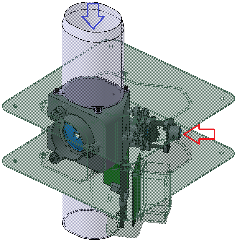
Figure 2The RCASS – a mechanical redesign of the UCASS (Smith et al., 2019). The red and blue arrows are the laser beam and airflow directions, respectively.
The mechanical redesign of the instrument also allowed an improvement of the internal aerodynamics. Smith et al. (2019) show CFD results used to determine operational limits for the instrument based on platform-velocity-derived mass concentration. However, the CFD simulations of the UCASS show an area of high stagnation pressure at the inlet on which a leading-edge vortex forms, directing particles around the sampling volume and thus altering the mass flux through the detector region. This effect can be seen in Fig. 3, which shows the flow profile through the UCASS for an input angle of attack of −20∘; this effect is demonstrable for all angles of attack (and in axial flow), but −20∘ is shown for the sake of brevity. This is amplified for negative angles of attack and high airspeeds (>10 m s−1), suggesting that the blunt geometry of the leading-edge face is causing this high gauge pressure and therefore the leading-edge vortex. Hence the RCASS inlet features a sharp tip similar to the “Korolev” cloud probe tips presented and simulated in Korolev et al. (2013). Although the Korolev tips are designed to prevent shattered ice particles from being sampled, the underlying process directing the ice particles into the sample volume is similar, with a high-pressure region forming on blunt tips, forcing ice shards into the sample volume. As shown by Jackson et al. (2014), the anti-shattering tips can impact historical data, demonstrating the need to assess artefacts of measurement retroactively. Another limitation with the UCASS is the positioning of the detector region in the boundary layer of the instrument, therefore causing particles to be sampled in a region with lowered airflow velocity and an increased likelihood of turbulent deposition. This is also shown in Fig. 3. The new design, therefore, features a sample area positioned farther away from the wall of the airflow tube. Following these results, the UCASS was also modified to include a collar around the inlet, which prevented the high pressure region from forming.
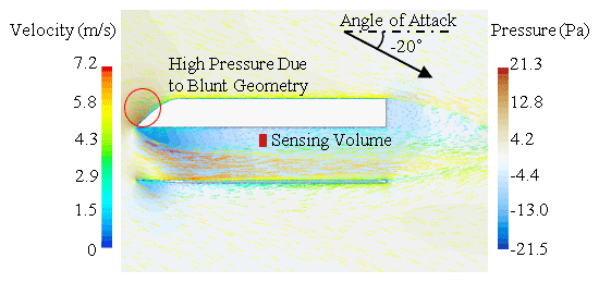
Figure 3A vector plot of CFD simulation results for the original UCASS with an airflow angle of attack of 20∘. The arrow represents angle of attack; the red circle is the high-pressure region, which directs particles around the sensing volume, labelled as a red square. The scale on the right is gauge pressure, corresponding to the colour of the background; the scale on the left is airflow velocity magnitude, corresponding to the colour of the glyphs.
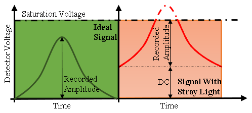
Figure 4An illustration of the effect of stray light on the signal output of the detector electronics (the transimpedance amplifier). Excess stray light will cause the Gaussian pulse from a particle to stray beyond the saturation point, represented in the red area of the figure.
Since the package had been changed, the stray-light issue (common among all OPCs, especially open-path) needed to be readdressed. The RCASS electronics can endure a certain amount of stray light using a direct current (DC) restoration circuit. This is an inverted peak detector circuit which will hold the value of the DC signal (a result of the stray light on the detector) minus any peaks from detected particles and noise. The DC signal is then subtracted from the total signal in a comparator. However, if the DC component is sufficiently large, the detector can start to saturate, exhibiting – in an ideal circuit – a Gaussian distribution with a flat top. Once the DC signal has been subtracted from this, the peaks appear smaller in amplitude, leading to the appearance of smaller particles – and eventually nothing – to be recorded. This effect is illustrated in Fig. 4. A stray-light test was devised on a prototype RCASS design, which was improved and verified following the tests. These tests are described in detail in Appendix B.
The original UCASS is available in two different gain modes: low gain to capture larger droplets (3 to 40 µm) and high gain to capture smaller droplets (0.4 to 20 µm). On the RCASS, a mechanical switch was installed to allow the operator to change the gain mode before a flight, depending on meteorological conditions.
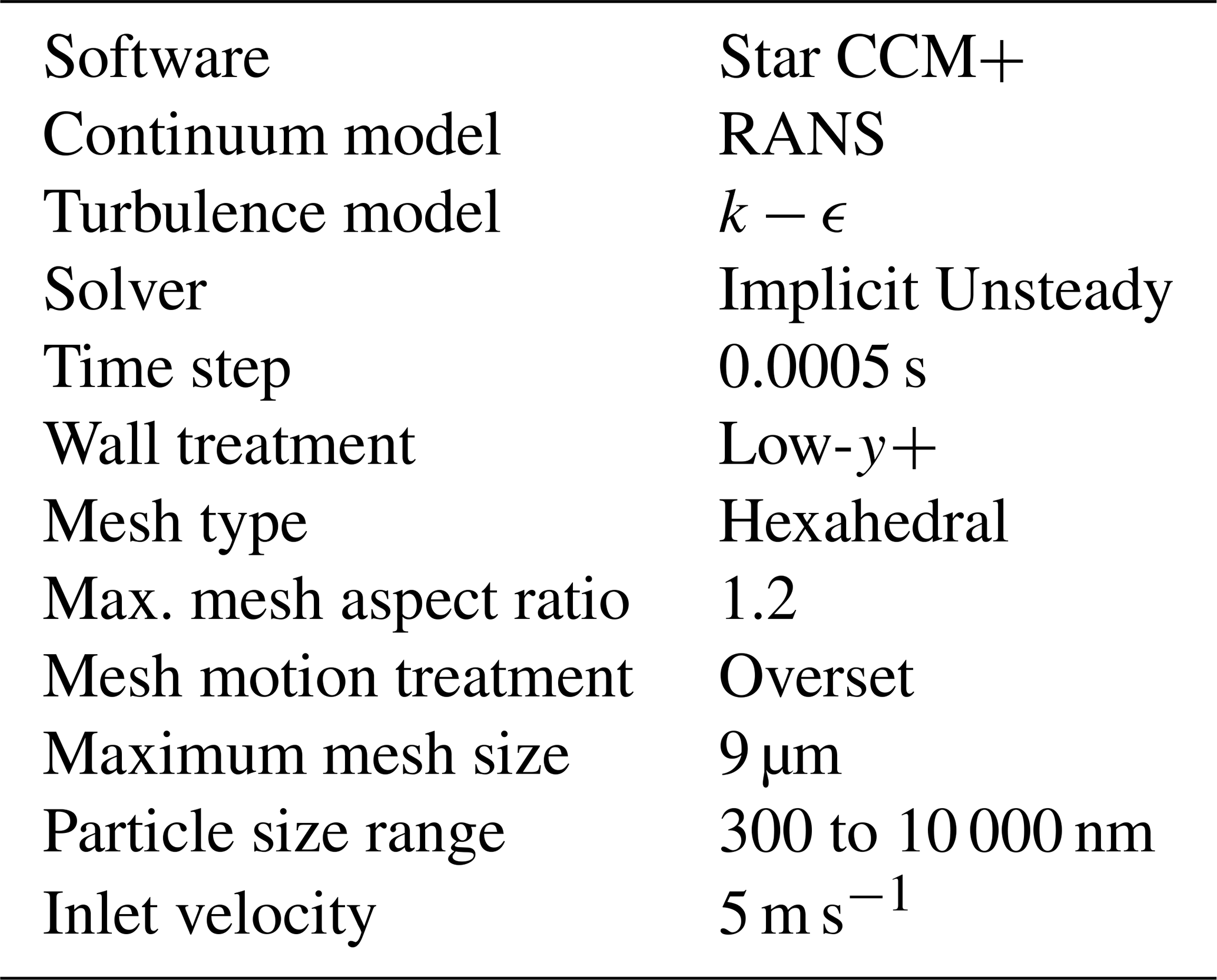
4.1 CFD–LPT methods
Simulations were performed to determine the best place on the SUA to position the RCASS. It was hypothesised that the minimal distortion of OPC measurement would be in the centre of the SUA; however a design compromise existed between the centralisation of the OPC or the Pixhawk flight controller. A centralised flight controller makes dynamic-stability tuning easier, but this may compromise OPC measurements. Previous works have used CFD as a design tool (for example Mckinney et al., 2019; Roldán et al., 2015); however the simulations used in this study are unique due to the Lagrangian particle tracking element.
Since the particle inlet is above the airframe, the aerodynamic effects of the airframe itself are negligible and therefore have been ignored. This also allows lower computation and meshing time. The simulation domain was a virtual wind tunnel consisting of a 4 m tall cylinder with a radius of 1.5 m; the eight propellers were positioned in this cylinder on a plane 2.5 m from the base. The centre of each propeller was located on the vertices of an octagon with an “across-flats” dimension of 0.97 m – the same geometry as the real SUA. The walls of the cylinder are assumed to generate no shear stress and hence no boundary layer. This was to simulate a quasi-free stream while simultaneously reducing computation time. Figure 5 shows a schematic of the CFD–LPT domain and propellers.
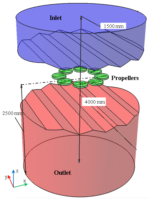
Figure 5This figure shows the CFD–LPT domain. Air and particles enter the domain at the top of the blue section labelled “Inlet” and flow downwards past the propellers. Each of the propellers is in a small green cylinder representing the overset mesh region; a section of the cylinder is cut away here for illustration purposes. Air and particles leave the domain through the bottom face of the cylinder in the red region.
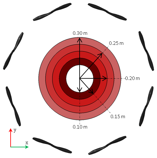
Figure 6This figure shows the particle sampling regions and their radii across one of the parallel sampling planes. The planes had z coordinates – relative to the propeller plane – between 0 and 0.3 m with an equal spacing of 0.05 m and were all identical. The propellers are shown here as a reference. The axis labelling system is consistent with Fig. 5.
The motion of the propellers was simulated using an overset mesh (also known as a “Chimera” mesh), which was chosen for its compatibility with the time-unsteady solver (required for LPT) and its flexibility with different mesh types. The transport equations used in the simulations were the Reynolds-averaged Navier Stokes (RANS) equations with a k−ϵ turbulence model. This is a two-equation eddy viscosity model, which is commonly used for its stability and accuracy in the free stream. The k−ϵ model tends to under-predict the anisotropy of turbulence near walls and in wakes; however the points of interest on the airframe were in the far field, away from walls. Tian and Ahmadi (2007) found that a Reynolds stress model (RSM) would more accurately predict near-wall turbulence conditions. However, in complex flows such as this, an RSM would be highly unstable and require minute time steps, which would vastly increase computation cost. While near-wall turbulence strongly influences turbulent deposition of particles, this effect was not expected to be important in this case since all areas of interest are far away from any boundary layers. Therefore, a k−ϵ turbulence model was sufficient.
These transport equations were solved numerically by an implicit unsteady solver, which was available in the “Star CCM+” commercial code used. This solver converges a simulation for each time step with multiple inner iterations (sub-steps). The quasi-time step for these inner iterations was calculated from a user-defined Courant number, which was set to 50; other internal Courant numbers were experimented with, but this was the best compromise between stability and computation time. The time step for all simulations was 0.0005 s, which was chosen to satisfy both the Courant–Friedrichs–Lewy (CFL) condition for the mesh size chosen and the Nyquist–Shannon sampling criterion for the motion of the propellers. Each simulation was run until it had converged, and the first particles injected into the simulation had left the domain. A sensitivity study was conducted to ensure the precision and reliability of the simulation results. This is presented in Appendix A.
The LPT component of the simulations used two models: a simple drag model to study the viscous and inertial forces exerted on the particles by the fluid and a turbulent dispersion model to study the effects of turbulence. Models that effect the particle size distribution – for example droplet break-up and coagulation – are not studied in these simulations due to their complexity and lack of validation. Instead, the droplet Weber number and fluid Reynolds number were calculated to ensure this did not happen (see Sect. 4.2). Particles in the simulation were “sampled” when their trajectory during one time step bisected a plane parallel with the x and y axes of the domain (parallel with the propeller plane shown in Fig. 5). These planes had z coordinates – relative to the propeller plane – between 0 and 0.3 m, with an equal spacing of 0.05 m, in addition to a control plane at the inlet to which the results were normalised. The planes were then split into five sampling regions, which were annular in shape with inner radii between 0 and 0.25 m (and a maximum outer radius of 0.3 m). These regions are shown in Fig. 6. Using the area of these regions and the number of particles passing through them per second, mass flux was derived as a convenient parameter to relate to OPC measurements. Mass flux was chosen over mass concentration so as to separate the artefacts generated by distortions in the trajectory of the particles, from the artefacts generated by deriving mass concentration from the velocity of the SUA.
Table 1Details of the model set-up for the CFD–LPT simulations.
If solid atmospheric particles – for example aerosolised Saharan dust – were to be modelled, electrostatic forces from a charged airframe would need to be considered to both scavenge and deflect these particles. In principle CFD–LPT could be combined with electrostatic modelling to characterise particle trajectories. However, the electrostatic portion of the model will be strongly dependant on the charge of an individual particle. This can significantly vary depending on aerosol type – and quantitative analysis of dust turbulent triboelectric charging, for example, is awaiting conclusions of ongoing research (Daskalopoulou et al., 2020). Also, the RCASS is mostly constructed from conductive materials, and all plastic parts were coated with RS Components 514-486 conductive anti-static spray; the RCASS chassis and inlet are grounded with respect to the main flight battery. This was done in order to reduce electrostatic-charging artefacts within the instrument itself.
The LPT simulations were run for a variety of particle sizes ranging from 300 to 10 000 nm (spaced quasi-logarithmically). This size range was chosen because it was predicted that smaller particles would be most affected by erroneous airflow due to their lower inertia. The results of these simulations are presented in Sect. 4.2.
4.2 CFD–LPT results and discussion
The simulated mass flux through the annular regions on a series of planes described in Sect. 4.1 is shown in Fig. 7. The plot shows the variation in mass flux with the z coordinate of the plane the regions are coincident to (or the elevation above the propellers). The mass flux ratio is the ratio of the mass flux through a region at the top of the domain (therefore unaffected by the propellers) to the mass flux in the same region at a different elevation. The purpose of this simulation was to determine the best location on the airframe for the OPC instrument. Since the OPC directly measures mass flux, Fig. 7 visualises the distortion in measurements due to the SUA propellers.
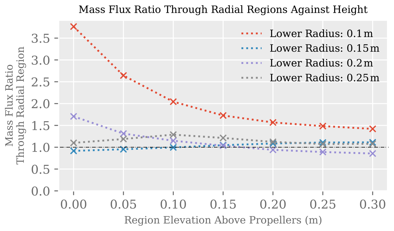
Figure 7CFD–LPT results for the ratio of particle mass flux at the top of the domain to particle mass flux through planes with varying z coordinates. Each line represents the mass flux through an annular region with a lower radius described in the key. The size of particle for this simulation is 300 nm.
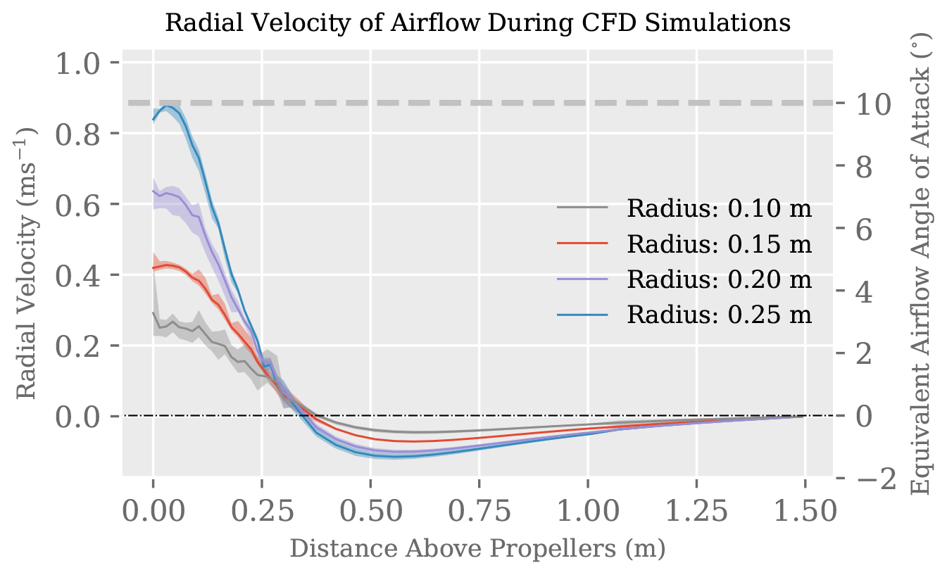
Figure 8CFD results for the (circumferentially averaged) radial velocity of the airflow as a function of distance above the propellers. The shaded regions around the lines show the variation in the air velocity around the circumference of the domain, while the bold lines show the mean. The dashed line represents the angle-of-attack limit specified in Smith et al. (2019).
Figure 7 shows a consistently higher mass flux ratio for the annular region in the centre of the domain, meaning fewer particles are passing through this area. This is because the propellers create a pressure gradient in the continuous phase, and the resulting drag force on the particles pushes them out from the centre. While this drag force is lowest at the centre region (since it is farthest from the propellers), it still shows consistently lower mass flux than the outer regions because the pressure gradient is forcing particles outward towards the propellers and is essentially “draining” the inner region. This is visualised in Fig. 8, which shows the circumferential average of the radial velocity (implying a radial pressure gradient since the radial velocity should be 0 if no other forces are acting on the continuum). Positive radial velocities in this figure mean airflow moving outwards from the centre towards the propellers, and positive radial velocities for all annular regions are shown with z coordinates lower than 0.3 m. Figure 8 also shows the angle of attack of the airflow with respect to the centre (z) axis of the domain. The purpose of this is to determine if the direction of the airflow is beyond the angle-of-attack limit of the UCASS sensor described in Smith et al. (2019) (10∘). While the airflow angle of attack at all points on this graph was acceptable, a lower “nominal” angle of attack will make the SUA more robust in crosswinds, which will further alter this variable. Additionally, the acceleration of the airflow close to the propellers and the high levels of turbulence in the continuous phase here mean the droplets are more likely to experience break-up effects. If a larger droplet was broken up into multiple smaller droplets – which were then sampled – the data products would show a shifted size distribution and a larger number concentration. According to Reitz (1987), the break-up conditions are given by
and
representing “bag” and “stripping” break-up, respectively. The Weber number of the droplets and Reynolds number of the flow are given by
and
respectively. The subscript 1 denotes the continuous phase and 2 the discrete phase. We is Weber number, Re is Reynolds number, ρ is density, v is velocity, dp is particle diameter, μ is dynamic viscosity, and σ is surface tension.
In both cases, the likelihood of the actual droplet sizes being altered is proportional to the square of the continuum velocity, which is likely to be higher closer to the propellers. Nevertheless, at all points in the analysed regions, neither the limit specified in Eq. (1) nor the limit in Eq. (2) was reached.
The induced change in continuous-phase temperature changing particle size was considered during the simulation analysis. However, the maximum change in temperature throughout all points considered for sampling – including parts along the full trajectory of a droplet – was 0.012 K. Since the vertical extent of this temperature field above the propeller plane is 0.8 m, a droplet would be exposed to this temperature field for 0.16 s, which is certainly not enough of a perturbation to cause any significant change in droplet size.
Figure 9 is intended to demonstrate the effect the propellers have on the particle size distribution. It was hypothesised that droplets with higher sizes (and hence larger inertia) would be less effected by the propellers. While Fig. 9 shows this is true, with the 10 000 nm size showing a mass flux ratio consistently closer to unity, the difference between the sizes is extremely small, with a mean standard deviation of 0.00097. This means that the propellers will have a small effect on the shape of the particle size distribution (PSD) when compared to its peak height. Not only does this make it easier to apply correction factors to measurements, but atmospheric phenomena, which only require measurements of a normalised PSD (e.g. Zeng, 2018), will be distorted by a negligible amount. Therefore, a correction factor to the particle size distribution is not required.
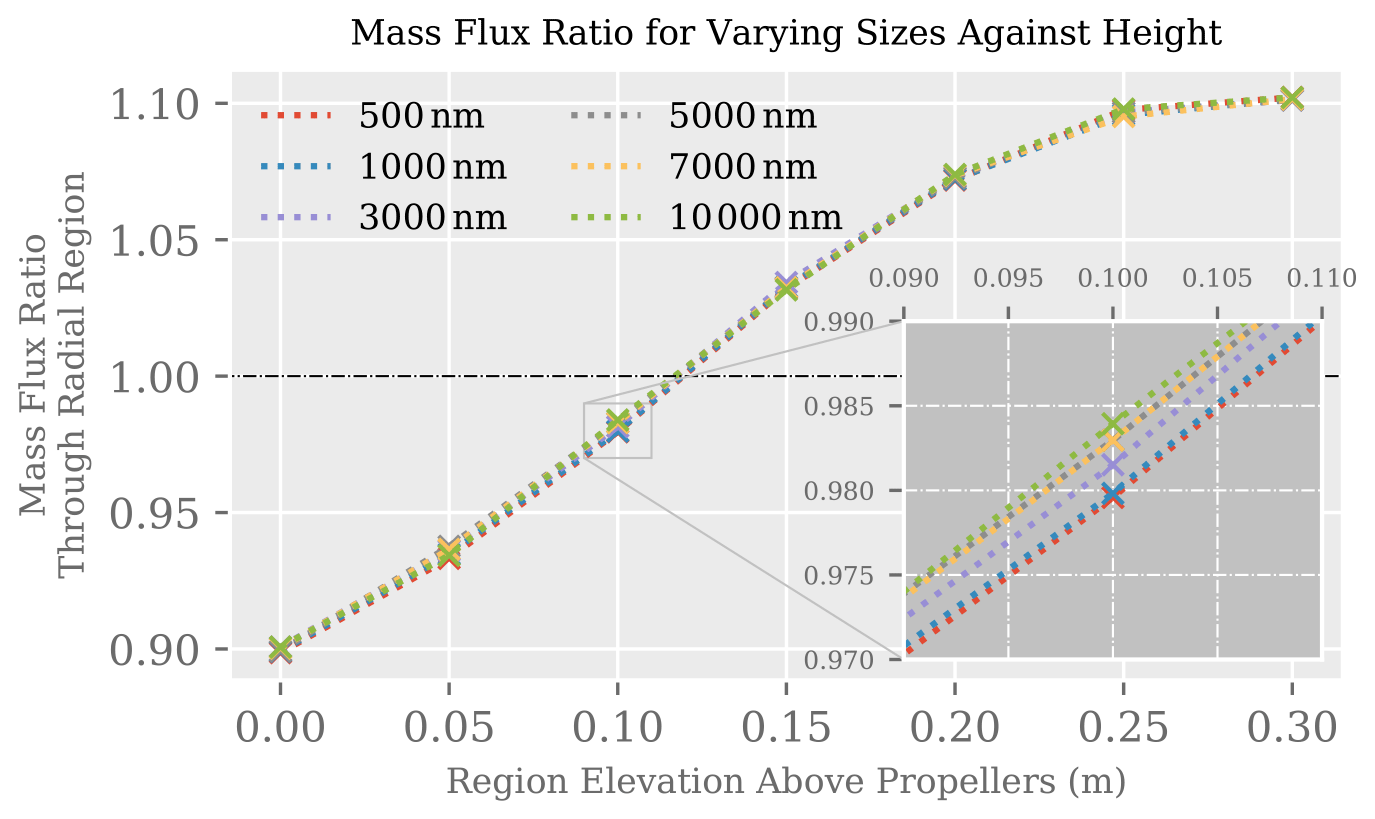
Figure 9CFD–LPT results for the ratio of particle mass flux at the top of the domain to particle mass flux through planes with varying z coordinates. Each line represents the mass flux for a different size particle described in the key. The annular region for this plot has a lower radius of 0.15 m and an upper radius of 0.2 m.
In contrast to most aerosol-sampling methods, the smaller aerosols with less inertia are more problematic in this situation due to the airflow acting to pull particles away from the OPC. However, when a crosswind is introduced, the larger particles would become more problematic with their greater inertia, causing them to impact against the walls of the RCASS. To reduce this artefact, the SUA can be allowed to drift with the wind when taking a vertical sampling profile with a crosswind. Smith et al. (2019) shows that the maximum angle of attack the UCASS can adapt to is 10∘; therefore the SUA will be drifting with the wind whenever a crosswind greater than approximately 1 m s−1 is expected, assuming an ascent rate of 5 m s−1. This, however, is not necessary for measurements of radiation fog since this phenomenon is typically associated with wind speeds less than 1 m s−1.
Figure 7 shows, for regional elevations greater than 0.15 m above the propellers, that lower regional radii between 0.15 m and 0.25 m (corresponding to an annulus with a lower radius of 0.15 m and an upper radius of 0.3 m) are acceptable. However, Fig. 8 shows larger radial velocities closer to the propellers. While these radial velocities are within the acceptable range for the UCASS, the addition of a crosswind would add to the maximum radial velocity. Therefore, the RCASS was positioned on the SUA on an annulus with a lower radius of 0.15 m and an upper radius of 0.2 m since this region exhibits the lowest average radial velocity.
5.1 Field test method
In order to evaluate the quality of the data collected by the UH-AeroSAM, a practical test was devised involving the comparison of SUA data with a calibrated in situ cloud probe. While conventionally the validation of simulation data is achieved using a wind tunnel and measurements of a scalar quantity (for example pressure), the size of UH-AeroSAM makes it difficult to find an appropriate tunnel, accounting for a mandated blockage ratio and wall distance. Also, a spatially homogeneous particle stream with a known size distribution in the tunnel is difficult to achieve, and various environmental factors (for example turbulence) are hard to simulate in a tunnel.
Since RCASS is an OPC, and thus accurate sizing of particles relies on a known refractive index and assumes a spherical shape, the material chosen for the validation was water droplets in low-level stratus (and fog). This minimised any uncertainty originating from an unknown particle refractive index, particles with unknown shape or non-homogeneous structures, or unknown artefacts resulting from surface roughness. Since both the RCASS and the reference instrumentation are OPCs, it may initially appear that these uncertainties would apply equally to both. However, different optical designs will capture different parts of a particle's phase function (most OPC cloud probes, including the cloud, aerosol, and precipitation spectrometer – CAPS – use forward scattering), which will not vary proportionally to each other with particle size.
The validation experiments were undertaken during the Pallas Cloud Experiment (PaCE) at the Pallas atmosphere–ecosystem supersite. This is located 170 km north of the Arctic Circle (67.973∘ N, 24.116∘ E), partly in the area of Pallas-Yllästunturi National Park (Lohila et al., 2015). A combination of a temporarily restricted airspace (D527 – Pallas), a common occurrence of low-level layered clouds (with a base of 300 to 500 m a.s.l., or 0 to 100 m above the SUA operations site), and the Sammaltunturi station made PaCE an ideal setting for the validation of UH-AeroSAM. For the duration of PaCE, a CAPS (Baumgardner et al., 2001) from Droplet Measurement Technologies (DMT) was positioned at the Sammaltunturi station at the peak of a hill. The CAPS, by default, is a naturally aspirated instrument which is unsuitable for static measurement, so a pump-and-inlet system was used to draw a sampling flow and turn it into an artificially aspirated instrument. The inlet to the CAPS was oriented into the wind for the duration of all flights. Details of this, along with evaluation, can be found in Doulgeris et al. (2020).
Between 20 and 28 September 2019, 24 sampling flights were conducted. However, due to a predominantly northerly wind, the Sammaltunturi station was only in the clouds on the 28th, when four flights were conducted, after which all flight batteries were depleted. The first flight was performed in “high-gain” mode (measuring smaller sizes). However, following on-site analysis of the data, it was found that a large proportion of the data appeared in the largest size bin, indicating that some particles were being undersized due to saturation of the detector. For this reason, the gain was reduced to “low-gain” mode for the remaining three flights, increasing the lower threshold to 1 µm and the higher threshold to 40 µm. The wind speed and direction on 28 September 2019 were 6 m s−1 and 240∘, respectively. The temperature at the station level on this date was 3.6 ∘C, so neither ice nor super-cooled water was expected.
In order to ensure quasi-Lagrangian measurements, the UH-AeroSAM was allowed to drift with the wind for all flights. The profiles were, therefore, slanted towards the station due to the 240∘ wind. The SUA operations site was approximately 450 m away from Sammaltunturi station – meaning the SUA was approximately 350 m away when its altitude corresponded to that of the station. The RCASS data for comparison were within the altitude range of 545 to 585 m a.s.l., which corresponds to the station altitude ±20 m.
5.2 Field test results and discussion
A comparison of normalised number concentration (dN∕dlog (Dp)) can be used to assess the performance of a particle instrument since it provides a size-resolved counting efficiency, and some particle loss mechanisms tend to be size-dependent. A comparative plot of normalised concentration for the SUA and CAPS is shown in Fig. 10. To reduce the significance of random artefacts, a 20 s arithmetic mean of the CAPS data and a 40 m arithmetic mean of the RCASS data were taken, centred on coinciding times and altitudes. This averaging period was chosen to cover the same temporal extent. The error margin in concentration for these data is taken to be 1 standard deviation over the averaged range; this is represented in Fig. 10 by error bars.
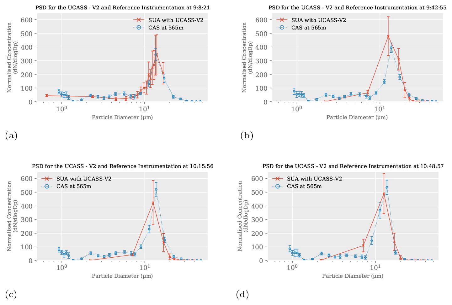
Figure 10Normalised concentration plots for the SUA flights on 28 September 2019. The first flight in (a) was conducted in high-gain mode, where it was observed that the largest particle size was beyond the transimpedance amplifier saturation point. The remaining three flights, therefore, were conducted in low-gain mode to ensure larger droplets were measured.
As a general statement, Fig. 10 shows that the RCASS in both gain modes and CAPS agree remarkably well. As outlined in Sect. 1, one aim of this paper is to outline an operational envelope where the SUA–OPC observations can be considered reliable. Therefore the discrepancies that do exist must be, at the very least, explained. The metric used here to compare the two instruments is the re-binned dN∕dlog (Dp), using the bin boundaries for the RCASS (since it has the lower resolution). This metric is indicative of both size and concentration discrepancies. Figure 11 shows the comparative plots for the re-binned data, the regression line, and the corresponding droplet diameter – using the geometric mean diameter of the bins – represented by the colour of the points. Reduced major axis regression (RMAR), as described in Harper (2016), was used since this technique correctly assumes that neither sampling method is perfect. Figure 11b is plotted on a log–log scale for clarity, leading to the appearance of a curved regression line. For Fig. 11b, sizes greater than 30 µm were neglected because, in all cases, both the CAPS and RCASS recorded zero concentration, which would give falsely strong correlation.
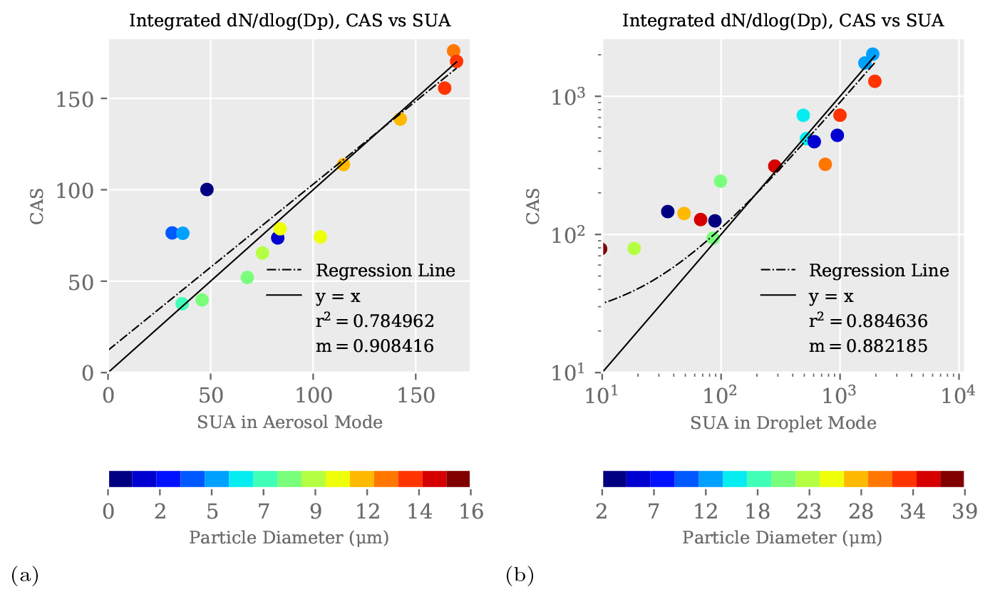
Figure 11Re-binned dN∕dlog (Dp) 1:1 plots. The solid line represents perfect agreement; the dotted line is the regression line using RMAR. The coefficient of determination is represented by r2, and m is the gradient of the regression line. In (b), a log–log scale was used since most values were close to 0; the appearance of a curved regression line in (b) is simply due to the log–log scale. The colour of the points corresponds to the bin geometric mean diameter, which is shown on the colour bar beneath the graph.
Figure 10a shows the only data collected in high-gain mode. This mode showed the best agreement with the CAPS, especially for sizes larger than 7 µm. Figure 11a shows a regression line gradient of 0.908 and an r2 of 0.785 for the re-binned dN∕dlog (Dp). However, these data show disagreement in two distinct places. The first is a dip in the CAPS data between 1 and 2 µm, which is undetected by RCASS. This is almost certainly due to the lower size resolution in this region since it is impossible for the two bins (centred around 0.6 and 2 µm) to capture this feature. The second is a peak in the CAPS data around 5 µm; similarly the CAPS data coincident to the other three flights on this day also detected this peak. The RCASS has sufficient resolution to capture this peak only in high-gain mode, but the only flight in high-gain mode did not capture this peak. Within the CAPS user community, the legitimacy of this peak tends to be questioned since it is often not detected by any other instrument. Certainly this could be an artificial double peak due to the highly non-monotonic nature of the Mie curve for a forward-scattering instrument; thus RCASS would not detect the peak with the more monotonic 60∘-centred (with a half angle of 44∘) scattering angle response curve (Smith et al., 2019). This could also be an artificial peak due to droplet shattering, although the small error margin compared to RCASS would indicate otherwise. Since this is not the topic for this paper, and this peak does not significantly affect the plots in Fig. 10, this part of the graph is not discussed further here.
Figure 10b, c, and d show all the data collected in low-gain mode. This instrument mode has a sufficient range to capture the entire major peak detected by the CAPS, and for the most part the two data sets agree well, although there are a few important points of discussion. The first is a lower resolution for smaller sizes, which causes the instrument to appear as though it disagrees. The worst case of this is presented in Fig. 10b. Since the high-gain mode agrees remarkably well with a higher resolution, and the only change between the two modes is a transimpedance amplifier gain, the issue can be resolved by adjusting the bin boundaries to give more resolution in this area during future measurements.
The second point is a concentration measured close to 0 in the first bin. This is likely due to the instrument's lower sensitivity to smaller sizes, characteristic of a typical OPC, where the sample volume is defined optically. Since the useful data products that would be calculated from the RCASS low-gain mode, for example liquid water content (LWC), would mostly rely on larger sizes, this error is insignificant for the most part. Nevertheless, the authors note that one would need to consider this effect when using data from sizes approaching the spectral limits of any OPC. It was considered that this effect could be due to smaller particles being pulled away from the propellers, as demonstrated in Sect. 4.2. However, this possibility was dismissed since the RCASS in high-gain mode did not suffer from this artefact, and this airflow effect would also affect all particle sizes equally.
The third, and most important, artefact is the drop-off in the concentration commonly observed by RCASS for sizes greater than 25 µm, which are particularly prominent in Fig. 10b. This is of utmost importance for parameters which rely on particle volume (for example LWC) since larger particles contribute more significantly to the total particle volume of a distribution than smaller ones. The suspected reason for this was that, while the SUA was allowed to drift with the wind, it is expected that a slip velocity exists between the airframe and the airflow. This slip velocity would become smaller in magnitude as the SUA ascends, assuming no wind shear. However, since the station is only 100 m above ground level, the slip velocity would likely not have been smaller than the 1 m s−1 limit calculated in Sect. 4.2. In future measurements, to compensate for this effect, the SUA could be preprogrammed to fly to a GPS waypoint, calculated so the horizontal speed of the airframe will match the wind speed. Flying upwards at faster speeds would also have the effect of increasing the aspiration efficiency of the instrument, although this might be detrimental to temperature and humidity measurements due to the slow response time of lightweight sensors introducing a lag in measurement. On the other hand, since this (size drop-off) discrepancy is mostly minute in these data, it could also easily be a co-location error. Larger droplets tend to accumulate near surface level in fog (as would be expected due to gravitational settling), which would explain the larger sizes measured by any instruments at the station. However, a more extensive data set would be needed to confirm this. Despite the minor artefacts, these data were remarkably accurate and precise, given the low instrument and platform cost.
In this paper, a novel design and validation technique for sampling aerosols on a multi-rotor SUA was presented. This research involved development and production of a bespoke SUA instrumented platform (UH-AeroSAM). The developmental work using both modelling and lab results found that placement of the particle instrument had a significant influence on the particle flux travelling through its sample volume. Along with the airframe, a bespoke OPC (RCASS) was developed with a naturally aspirated inlet, specifically for use on SUA. This OPC was based on the single-use UCASS (Smith et al., 2019) and incorporated several improvements to the sample airflow, electrical design, and mechanical robustness. The SUA is intended to fly vertically with the OPC inlet pointed upwards to achieve a vertical profile of atmospheric aerosol or droplets. RCASS can function in two gain modes: high-gain to measure smaller sizes with high resolution and low-gain to measure larger sizes with lower resolution.
The primary tool used in the design process was computational fluid dynamics with Lagrangian particle tracking (CFD–LPT); this revealed the physical processes affecting the flow of particles through the system. When the airflow is axial with respect to the SUA, the propellers create a lower pressure above the propellers and draw particles towards them. This was shown to effect all sizes measured by the RCASS equally. The CFD–LPT simulations revealed a significantly changing particle flux across the airframe due to the propellers; these simulations influenced the positioning of the particle counter on the airframe. An adequately compromised position was found using this method, and the SUA was constructed according to these specifications.
UH-AeroSAM was evaluated in a realistic field campaign setting using the cloud, aerosol, and precipitation spectrometer from Droplet Measurement Technologies as a reference. Across the whole measurement range, the two instruments showed excellent agreement in both RCASS gain modes.
This research delivers hitherto the next step in regular, reliable, and accurate SUA-based measurements of particulate and droplet spectra. This is a quantity regularly desired in many fields of atmospheric research but notoriously difficult to measure on SUA due to the large number of uncharacterised artefacts. However, with the measurement technique presented in this paper, the UH-AeroSAM is capable of accurately measuring the vertically resolved droplet spectra of fog and low-level clouds. This could also be extended to measure particulate matter (PM) concentration and low-level dust loading.
Future research will include adapting the RCASS for fixed-wing platforms and characterising the artefacts encountered. While multi-rotor SUA have better spatio-temporal sampling capabilities, a fixed-wing SUA with a similar maximum take-off mass (MTOM) would have a larger payload mass and longer endurance. Therefore, it is necessary to explore both applications for different uses.
To ensure the precision and reliability of simulation results, a mesh sensitivity study was conducted. The CFD domain described in Sect. 4.1 was used without the LPT models since these are not affected by the mesh. The mesh size was varied between 5 and 13 µm and run for the minimum convergence time, which was found during trials to be 30 time steps. All simulations were run on the University of Hertfordshire High-Power Cluster (UHHPC) on 64 processors in parallel.
The quantity chosen here to compare the different mesh sizes was the velocity magnitude – spatially averaged across the circumference of circles (concentric with the domain cylinder) with varying radii and distance above the propellers. The chosen radii (r) were 0.1, 0.2, and 0.3 metres on a plane parallel with the propellers. The distance (z) above the propellers was varied up to the top of the domain in intervals of 0.05 m. This positioning was chosen because it is the region of interest for the real simulations. This quantity () was normalised to the co-located in the simulation with the finest mesh size – 5 µm – to obtain velocity deviation (). The subscript 0 denotes the simulation with the finest mesh size, and i denotes the simulation with mesh size “i”. The purpose of the spatial (circumferential) average was to avoid differences in velocity magnitude between time steps due to the position of the propellers, which would exist naturally and give misleading results. The spacing of the circles give 93 values of per simulation. These data, along with CPU time for each simulation, are presented in Fig. A1. The CPU time for the simulation with an 8 µm mesh – the red circle in Fig. A1 – was dismissed as anomalous due to high UHHPC usage at the time this simulation was conducted.
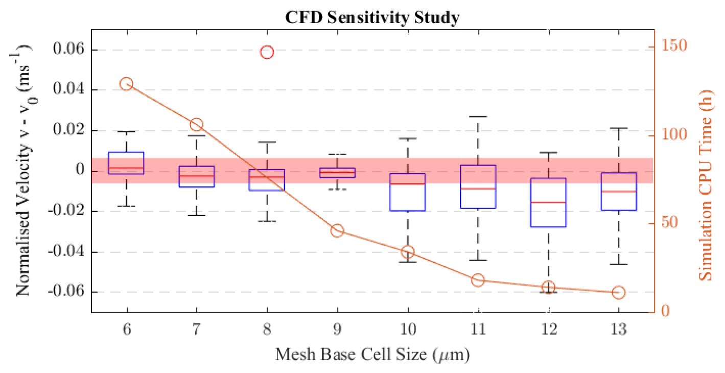
Figure A1A box-and-whisker plot representation of the CFD sensitivity study results. The whiskers represent the range of the data, the boxes represent the interquartile range, and the lines represent the mean. On the left vertical axis is the velocity magnitude normalised to the co-located point in the simulation with the finest mesh size (5 µm). The horizontal is the base mesh size. The right vertical axis is the simulation CPU time in hours. The shaded red region represents the valid region for the mean normalised velocity magnitude.
To determine which simulation to use, a limit for the mean velocity deviation had to be established. Here, this limit was defined as the velocity which produces a dynamic pressure capable of moving a particle across 1∕10th of a sampling region (0.01 m) when applied constantly from the inlet to the propeller plane (for 0.3 s when travelling 1.5 m at 5 m s−1). This problem can be reduced to one dimension if the pressure is applied constantly as the particle travels in the vertical direction. Therefore the particle must not travel 0.01 m in 0.3 s laterally. The largest mean velocity deviation calculated for a simulation was ±0.0063 m s−1, using Newtonian equations of motion and assuming Stokes flow. This limit is shown in Fig. A1 as a red-shaded valid region.
The coarsest mesh that lies within this limit had a base size of 9 µm and was therefore used for the main CFD–LPT simulations.
As an analogue to the sun, a 12 V halogen bulb with a parabolic directional reflector was used as the stray-light source due to its similar spectrum. From previous tests on both the UCASS and RCASS, it was found that stray light had the largest effect with an unobstructed path to the detector. Therefore the RCASS was rigidly mounted with a halogen bulb pointing directly at the detector, corresponding to a solar zenith angle of 25∘ when mounted in the SUA. To measure the equivalent solar power, a laser power meter (calibrated to 500 nm, in the middle of the solar spectrum) was used to measure the radiant flux of the halogen light. This was done to make the measurements comparable to true solar irradiance in order to define a suitable operating envelope for sampling with the SUA. From initial testing, it was found that the RCASS was unaffected by stray light resulting from a halogen bulb voltage of less then 3.1 V and completely saturated by bulb voltages more than 4 V. The voltage was therefore varied between 3 and 4 V in steps of 0.1 V, and the irradiance was measured at each data point.
For this experiment, polydisperse water droplets were used as the measurand because of their quasi-spherical shape – so they can be modelled using Mie theory – and ease of generation. A compressed-air-droplet generator was rigidly mounted for consistency between experiments. A fan was positioned behind the droplet source, causing a 1.8 m s−1 airflow through the RCASS. For each iteration of the experiment, the water droplets were sprayed into the instrument for 9 s. The bin boundaries for the test are spaced logarithmically between 0 and 4095 (for the 12-bit analogue-to-digital converter, ADC).
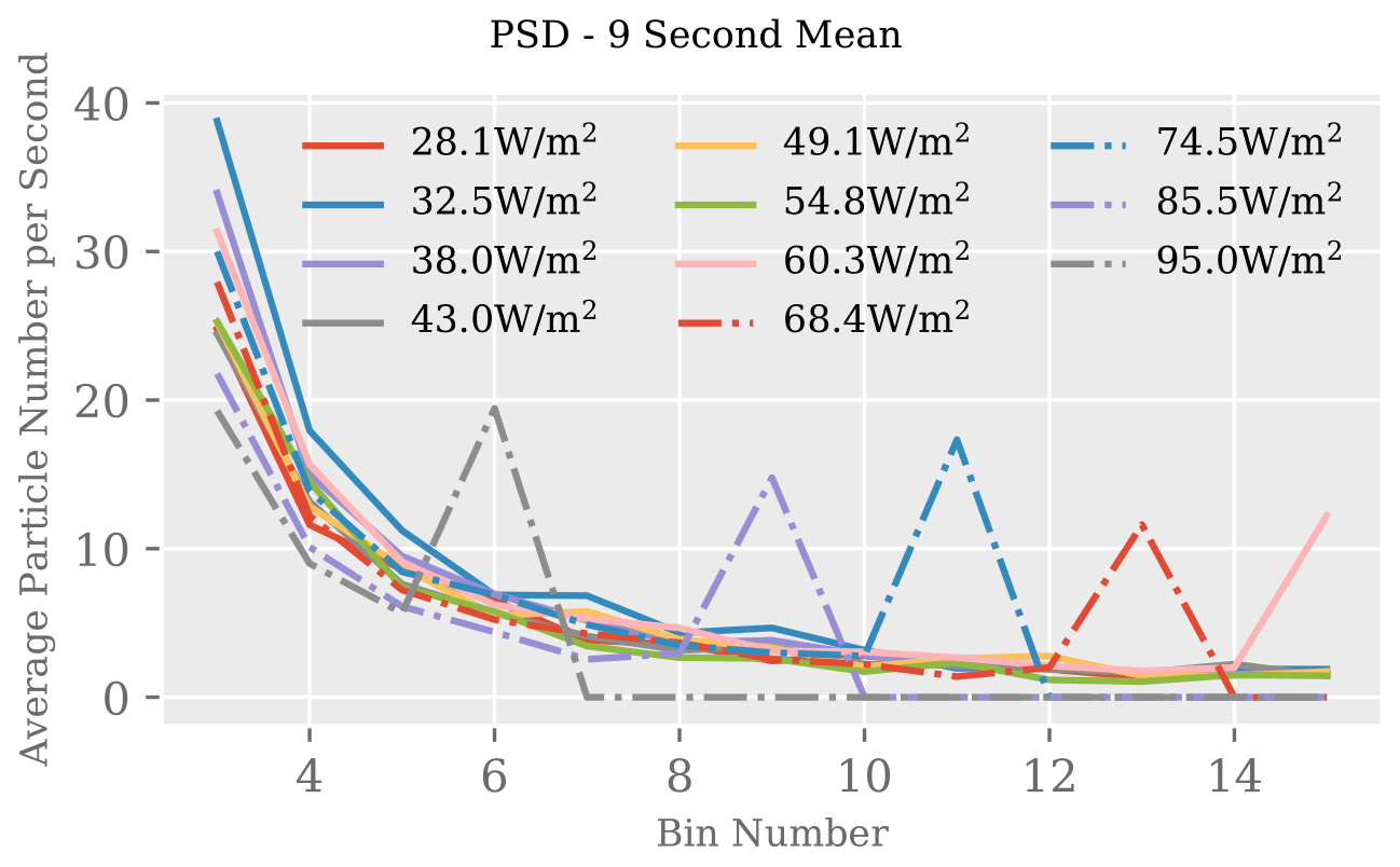
Figure B1The results from the RCASS stray-light test. Each line on this graph represents a different irradiance from the halogen bulb used as an analogue to the sun. Irradiances larger than this were found to completely saturate the photodiode and cause no counts to be registered.
Figure B1 shows the results from the stray-light test. The vertical axis represents the particle counts per second averaged over the 9 s period the droplets were being sprayed, and the horizontal axis is the bin number of the OPC. The different lines on the plot represent the changing solar-equivalent irradiance. This plot clearly demonstrates the saturation of the photodiode for irradiances larger than 60 W m−2. For example, with the halogen bulb at 95 W m−2, there is a peak at bin 6, followed by no counts at all for the higher bins. This is because, for the DC signal at 95 W m−2, the largest peak possible is “binned” at a 12-bit ADC value corresponding to bin 6 (578 in this case), and all other particles which would normally – with no stray light – generate larger peaks, are “binned” here.
Although the effective zenith angular range is small, it was decided post-test that the inlet should be extended so no direct path was available for stray light to reach the detector. This test also revealed that the plastic used for some of the bodywork transmitted infrared radiation, to which the RCASS detector is highly sensitive, so gold foil was used to surround the inlet exterior and reflect infrared.
The data for the CFD–LPT simulations are available here: https://doi.org/10.17632/7by3d28hxf.1 (Girdwood, 2020b). The CAPS and SUA data for the 28 September 2019 (during the PaCE 2019 campaign) are publicly available here: https://doi.org/10.17632/htbxftpc9h.1 (Girdwood, 2020a). The code used for the PaCE campaign data analysis is available here: https://github.com/JGirdwood/AeroSAM-Analysis (last access: 27 November 2020, JGirdwood, 2019).
The original draft manuscript was prepared by JG and reviewed and edited by all co-authors. Funding was acquired by JG (Aerosol Society travel award). The project was conceptualised by HS, ZU, WS, CS, DC, and JG. Data curation was conducted by JG, DB, and KMD. Formal analysis was conducted by JG. Project supervision was the responsibility of HS, WS, ZU, CS, and CC. Methodology was developed by JG, ZU, DB, and RM. Validation was conducted by JG. Software was created by JG and WS.
The authors declare that they have no conflict of interest.
We thank the Finnish Meteorological Institute for providing accommodation and logistics throughout the Pallas Cloud Experiment. Travel and shipping were subsidised by a travel award from the Aerosol Society. We also thank the UK Met Office Meteorological Research Unit at Cardington for providing support in temperature and humidity instrumentation calibration and flight testing.
This paper was edited by Troy Thornberry and reviewed by two anonymous referees.
3DRobotics: Pixhawk 1.2, available at: https://pixhawk.org/ (last access: 12 January 2020), 2013. a
Altstädter, B., Platis, A., Wehner, B., Scholtz, A., Wildmann, N., Hermann, M., Käthner, R., Baars, H., Bange, J., and Lampert, A.: ALADINA – an unmanned research aircraft for observing vertical and horizontal distributions of ultrafine particles within the atmospheric boundary layer, Atmos. Meas. Tech., 8, 1627–1639, https://doi.org/10.5194/amt-8-1627-2015, 2015. a, b
Altstädter, B., Platis, A., Jähn, M., Baars, H., Lückerath, J., Held, A., Lampert, A., Bange, J., Hermann, M., and Wehner, B.: Airborne observations of newly formed boundary layer aerosol particles under cloudy conditions, Atmos. Chem. Phys., 18, 8249–8264, https://doi.org/10.5194/acp-18-8249-2018, 2018. a, b
Alvarado, M., Gonzalez, F., Erskine, P., Cliff, D., and Heuff, D.: A Methodology to Monitor Airborne PM10 Dust Particles Using a Small Unmanned Aerial Vehicle, Sensors, 17, 343, https://doi.org/10.3390/s17020343, 2017. a, b
Baars, H., Kanitz, T., Engelmann, R., Althausen, D., Heese, B., Komppula, M., Preißler, J., Tesche, M., Ansmann, A., Wandinger, U., Lim, J.-H., Ahn, J. Y., Stachlewska, I. S., Amiridis, V., Marinou, E., Seifert, P., Hofer, J., Skupin, A., Schneider, F., Bohlmann, S., Foth, A., Bley, S., Pfüller, A., Giannakaki, E., Lihavainen, H., Viisanen, Y., Hooda, R. K., Pereira, S. N., Bortoli, D., Wagner, F., Mattis, I., Janicka, L., Markowicz, K. M., Achtert, P., Artaxo, P., Pauliquevis, T., Souza, R. A. F., Sharma, V. P., van Zyl, P. G., Beukes, J. P., Sun, J., Rohwer, E. G., Deng, R., Mamouri, R.-E., and Zamorano, F.: An overview of the first decade of PollyNET: an emerging network of automated Raman-polarization lidars for continuous aerosol profiling, Atmos. Chem. Phys., 16, 5111–5137, https://doi.org/10.5194/acp-16-5111-2016, 2016. a
Bärfuss, K., Pätzold, F., Altstädter, B., Kathe, E., and Nowak, S.: New Setup of the UAS ALADINA for Measuring Boundary Layer Properties, Atmospheric Particles and Solar Radiation, Atmosphere, 9, 28, https://doi.org/10.3390/atmos9010028, 2018. a
Bates, T. S., Quinn, P. K., Johnson, J. E., Corless, A., Brechtel, F. J., Stalin, S. E., Meinig, C., and Burkhart, J. F.: Measurements of atmospheric aerosol vertical distributions above Svalbard, Norway, using unmanned aerial systems (UAS), Atmos. Meas. Tech., 6, 2115–2120, https://doi.org/10.5194/amt-6-2115-2013, 2013. a, b
Baumgardner, D. and Spowart, M.: Evaluation of the Forward Scattering Spectrometer Probe. Part III: Time Response and Laser Inhomogeneity Limitations, J. Atmos. Ocean. Tech., 7, 666–672, https://doi.org/10.1175/1520-0426(1990)007<0666:EOTFSS>2.0.CO;2, 1990. a
Baumgardner, D., Strapp, W., and Dye, J. E.: Evaluation of the Forward Scattering Spectrometer Probe. Part II: Corrections for Coincidence and Dead-Time Losses, J. Atmos. Ocean. Tech., 2, 626–632, https://doi.org/10.1175/1520-0426(1985)002<0626:EOTFSS>2.0.CO;2, 1985. a
Baumgardner, D., Jonsson, H., Dawson, W., O'Connor, D., and Newton, R.: The cloud, aerosol and precipitation spectrometer: A new instrument for cloud investigations, Atmos. Res., 59–60, 251–264, https://doi.org/10.1016/S0169-8095(01)00119-3, 2001. a
Beswick, K., Baumgardner, D., Gallagher, M., Volz-Thomas, A., Nedelec, P., Wang, K.-Y., and Lance, S.: The backscatter cloud probe – a compact low-profile autonomous optical spectrometer, Atmos. Meas. Tech., 7, 1443–1457, https://doi.org/10.5194/amt-7-1443-2014, 2014. a
Bokoye, A. I., Royer, A., O'Neill, N. T., and Bruce McArthur, L. J.: A North American Arctic aerosol climatology using ground-based sunphotometry, Arctic, 55, 215–228, 2002. a
Buschmann, M., Bange, J., and Vörsmann, P.: MMAV-a miniature unmanned aerial vehicle (Mini-UAV) for meteorological purposes, in: Proceedings of the 16th Symposium on Boundary Layers and Turbulence, Rhode Island, 10 August 2004. a
Che, H., Zhang, X., Chen, H., Damiri, B., Goloub, P., Li, Z., Zhang, X., Wei, Y., Zhou, H., Dong, F., Li, D., and Zhou, T.: Instrument calibration and aerosol optical depth validation of the China aerosol remote sensing network, J. Geophys. Res., 114, D03206, https://doi.org/10.1029/2008JD011030, 2009. a
Clarke, A. D., Ahlquist, N. C., Howell, S., and Moore, K.: A miniature optical particle counter for in situ aircraft aerosol research, J. Atmos. Ocean. Tech., 19, 1557–1566, https://doi.org/10.1175/1520-0426(2002)019<1557:AMOPCF>2.0.CO;2, 2002. a
Corrigan, C. E., Roberts, G. C., Ramana, M. V., Kim, D., and Ramanathan, V.: Capturing vertical profiles of aerosols and black carbon over the Indian Ocean using autonomous unmanned aerial vehicles, Atmos. Chem. Phys., 8, 737–747, https://doi.org/10.5194/acp-8-737-2008, 2008. a
Daskalopoulou, V., Mallios, S. A., Ulanowski, Z., Hloupis, G., Gialitaki, A., Tassis, K., and Amiridis, V.: The Electrical Activity of Saharan Dust as perceived from Surface Electric Field Observations in Greece, Atmos. Chem. Phys. Discuss., https://doi.org/10.5194/acp-2020-668, in review, 2020. a
Doulgeris, K.-M., Komppula, M., Romakkaniemi, S., Hyvärinen, A.-P., Kerminen, V.-M., and Brus, D.: In situ cloud ground-based measurements in the Finnish sub-Arctic: intercomparison of three cloud spectrometer setups, Atmos. Meas. Tech., 13, 5129–5147, https://doi.org/10.5194/amt-13-5129-2020, 2020. a
Drury, E., Jacob, D. J., Spurr, R. J., Wang, J., Shinozuka, Y., Anderson, B. E., Clarke, A. D., Dibb, J., McNaughton, C., and Weber, R.: Synthesis of satellite (MODIS), aircraft (ICARTT), and surface (IMPROVE, EPA-AQS, AERONET) aerosol observations over eastern North America to improve MODIS aerosol retrievals and constrain surface aerosol concentrations and sources, J. Geophys. Res., 115, D14204, https://doi.org/10.1029/2009JD012629, 2010. a
Dye, J. E. and Baumgardner, D.: Evaluation of the Forward Scattering Spectrometer Probe. Part I: Electronic and Optical Studies, J. Atmos. Ocean. Tech., 1, 329–344, https://doi.org/10.1175/1520-0426(1984)001<0329:EOTFSS>2.0.CO;2, 1984. a
Egli, S., Maier, F., Bendix, J., and Thies, B.: Vertical distribution of microphysical properties in radiation fogs – A case study, Atmos. Res., 151, 130–145, https://doi.org/10.1016/j.atmosres.2014.05.027, 2015. a
Gao, R. S., Perring, A. E., Thornberry, T. D., Rollins, A. W., Schwarz, J. P., Ciciora, S. J., and Fahey, D. W.: A high-sensitivity low-cost optical particle counter design, Aerosol Sci. Tech., 47, 137–145, https://doi.org/10.1080/02786826.2012.733039, 2013. a
Gao, R. S., Telg, H., McLaughlin, R. J., Ciciora, S. J., Watts, L. A., Richardson, M. S., Schwarz, J. P., Perring, A. E., Thornberry, T. D., Rollins, A. W., Markovic, M. Z., Bates, T. S., Johnson, J. E., and Fahey, D. W.: A light-weight, high-sensitivity particle spectrometer for PM2.5 aerosol measurements, Aerosol Sci. Tech., 50, 88–99, https://doi.org/10.1080/02786826.2015.1131809, 2016. a
Girdwood, J.: PaCE-2019-UHAeroSAM-CAPS, Mendeley Data, V1, https://doi.org/10.17632/htbxftpc9h.1, 2020a. a
Girdwood, J.: UHAeroSAM-CFTLPT, Mendeley Data, V1, https://doi.org/10.17632/7by3d28hxf.1, 2020b. a
Greene, B. R., Segales, A. R., Waugh, S., Duthoit, S., and Chilson, P. B.: Considerations for temperature sensor placement on rotary-wing unmanned aircraft systems, Atmos. Meas. Tech., 11, 5519–5530, https://doi.org/10.5194/amt-11-5519-2018, 2018. a
Hara, K., Iwasaka, Y., Wada, M., Ihara, T., Shiba, H., Osada, K., and Yamanouchi, T.: Aerosol constituents and their spatial distribution in the free troposphere of coastal Antarctic regions, J. Geophys. Res., 111, D15216, https://doi.org/10.1029/2005JD006591, 2006. a
Harper, W. V.: Reduced Major Axis Regression, in: Wiley StatsRef: Statistics Reference Online, edited by: Balakrishnan, N., Colton, T., Everitt, B., Piegorsch, W., Ruggeri, F., and Teugels, J. L., John Wiley & Sons, Ltd, Chichester, UK, 9, 1–6, https://doi.org/10.1002/9781118445112.stat07912, 2016. a
IPCC: The Physical Science Basis: Contribution of Working Group 1 to the Fifth Assessment Report of the IPCC, Cambridge University Press, Cambridge, 2013. a
Jackson, R. C., Mcfarquhar, G. M., Stith, J., Beals, M., Shaw, R. A., Jensen, J., Fugal, J., and Korolev, A.: An assessment of the impact of antishattering tips and artifact removal techniques on cloud ice size distributions measured by the 2D cloud probe, J. Atmos. Ocean. Tech., 31, 2567–2590, https://doi.org/10.1175/JTECH-D-13-00239.1, 2014. a
JGirdwood: AeroSAM-Analysis, GitHub, available at: https://github.com/JGirdwood/AeroSAM-Analysis (last access: 27 November 2020), 2019. a
Korolev, A., Emery, E., and Creelman, K.: Modification and tests of particle probe tips to mitigate effects of ice shattering, J. Atmos. Ocean. Tech., 30, 690–708, https://doi.org/10.1175/JTECH-D-12-00063.1, 2013. a
Lance, S., Brock, C. A., Rogers, D., and Gordon, J. A.: Water droplet calibration of the Cloud Droplet Probe (CDP) and in-flight performance in liquid, ice and mixed-phase clouds during ARCPAC, Atmos. Meas. Tech., 3, 1683–1706, https://doi.org/10.5194/amt-3-1683-2010, 2010. a
Lohila, A., Penttilä, T., Jortikka, S., Aalto, T., Anttila, P., Asmi, E., Aurela, M., Hatakka, J., Hellén, H., Henttonen, H., Hänninen, P., Kilkki, J., Kyllönen, K., Laurila, T., Lepistö, A., Lihavainen, H., Makkonen, U., Paatero, J., Rask, M., Sutinen, R., Tuovinen, J. P., Vuorenmaa, J., and Viisanen, Y.: Preface to the special issue on integrated research of atmosphere, ecosystems and environment at Pallas, Boreal Environ. Res., 20, 431–454, 2015. a, b
Mamali, D., Marinou, E., Sciare, J., Pikridas, M., Kokkalis, P., Kottas, M., Binietoglou, I., Tsekeri, A., Keleshis, C., Engelmann, R., Baars, H., Ansmann, A., Amiridis, V., Russchenberg, H., and Biskos, G.: Vertical profiles of aerosol mass concentration derived by unmanned airborne in situ and remote sensing instruments during dust events, Atmos. Meas. Tech., 11, 2897–2910, https://doi.org/10.5194/amt-11-2897-2018, 2018. a, b
Martin, S., Bange, J., and Beyrich, F.: Meteorological profiling of the lower troposphere using the research UAV “M2AV Carolo”, Atmos. Meas. Tech., 4, 705–716, https://doi.org/10.5194/amt-4-705-2011, 2011. a
McKinney, K. A., Wang, D., Ye, J., de Fouchier, J.-B., Guimarães, P. C., Batista, C. E., Souza, R. A. F., Alves, E. G., Gu, D., Guenther, A. B., and Martin, S. T.: A sampler for atmospheric volatile organic compounds by copter unmanned aerial vehicles, Atmos. Meas. Tech., 12, 3123–3135, https://doi.org/10.5194/amt-12-3123-2019, 2019. a
Platis, A., Altstädter, B., Wehner, B., Wildmann, N., Lampert, A., Hermann, M., Birmili, W., and Bange, J.: An Observational Case Study on the Influence of Atmospheric Boundary-Layer Dynamics on New Particle Formation, Bound.-Lay. Meteorol., 158, 67–92, https://doi.org/10.1007/s10546-015-0084-y, 2016. a
Ramanathan, V., Ramana, M. V., Roberts, G., Kim, D., Corrigan, C., Chung, C., and Winker, D.: Warming trends in Asia amplified by brown cloud solar absorption, Nature, 448, 575–578, https://doi.org/10.1038/nature06019, 2007. a
RaspberryPi-Foundation: Raspberry Pi Zero, available at: https://www.raspberrypi.org/products/raspberry-pi-zero/ (last access: 12 January 2020), 2015. a
Reitz, D.: Modeling Atomization Processes in High-Pressure Vaporizing Sprays, Atomisation and Spray Technology, 3, 309–337, 1987. a
Renard, J.-B., Dulac, F., Berthet, G., Lurton, T., Vignelles, D., Jégou, F., Tonnelier, T., Jeannot, M., Couté, B., Akiki, R., Verdier, N., Mallet, M., Gensdarmes, F., Charpentier, P., Mesmin, S., Duverger, V., Dupont, J.-C., Elias, T., Crenn, V., Sciare, J., Zieger, P., Salter, M., Roberts, T., Giacomoni, J., Gobbi, M., Hamonou, E., Olafsson, H., Dagsson-Waldhauserova, P., Camy-Peyret, C., Mazel, C., Décamps, T., Piringer, M., Surcin, J., and Daugeron, D.: LOAC: a small aerosol optical counter/sizer for ground-based and balloon measurements of the size distribution and nature of atmospheric particles – Part 2: First results from balloon and unmanned aerial vehicle flights, Atmos. Meas. Tech., 9, 3673–3686, https://doi.org/10.5194/amt-9-3673-2016, 2016. a
Renard, J.-B., Dulac, F., Durand, P., Bourgeois, Q., Denjean, C., Vignelles, D., Couté, B., Jeannot, M., Verdier, N., and Mallet, M.: In situ measurements of desert dust particles above the western Mediterranean Sea with the balloon-borne Light Optical Aerosol Counter/sizer (LOAC) during the ChArMEx campaign of summer 2013, Atmos. Chem. Phys., 18, 3677–3699, https://doi.org/10.5194/acp-18-3677-2018, 2018. a
Reuder, J., Brisset, P., Jonassen, M., Müller, M., and Mayer, S.: The Small Unmanned Meteorological Observer SUMO: A new tool for atmospheric boundary layer research, Meteorol. Z., 18, 141–147, https://doi.org/10.1127/0941-2948/2009/0363, 2009. a
Roldán, J. J., Joossen, G., Sanz, D., del Cerro, J., and Barrientos, A.: Mini-UAV based sensory system for measuring environmental variables in greenhouses, Sensors, 15, 3334–3350, https://doi.org/10.3390/s150203334, 2015. a
Smith, H. R., Ulanowski, Z., Kaye, P. H., Hirst, E., Stanley, W., Kaye, R., Wieser, A., Stopford, C., Kezoudi, M., Girdwood, J., Greenaway, R., and Mackenzie, R.: The Universal Cloud and Aerosol Sounding System (UCASS): a low-cost miniature optical particle counter for use in dropsonde or balloon-borne sounding systems, Atmos. Meas. Tech., 12, 6579–6599, https://doi.org/10.5194/amt-12-6579-2019, 2019. a, b, c, d, e, f, g, h, i, j
Tian, L. and Ahmadi, G.: Particle deposition in turbulent duct flows–comparisons of different model predictions, J. Aerosol Sci., 38, 377–397, https://doi.org/10.1016/j.jaerosci.2006.12.003, 2007. a
Tsekeri, A., Lopatin, A., Amiridis, V., Marinou, E., Igloffstein, J., Siomos, N., Solomos, S., Kokkalis, P., Engelmann, R., Baars, H., Gratsea, M., Raptis, P. I., Binietoglou, I., Mihalopoulos, N., Kalivitis, N., Kouvarakis, G., Bartsotas, N., Kallos, G., Basart, S., Schuettemeyer, D., Wandinger, U., Ansmann, A., Chaikovsky, A. P., and Dubovik, O.: GARRLiC and LIRIC: strengths and limitations for the characterization of dust and marine particles along with their mixtures, Atmos. Meas. Tech., 10, 4995–5016, https://doi.org/10.5194/amt-10-4995-2017, 2017. a, b
van den Kroonenberg, A., Martin, T., Buschmann, M., Bange, J., and Vörsmann, P.: Measuring the wind vector using the autonomous mini aerial vehicle M2AV, J. Atmos. Ocean. Tech., 25, 1969–1982, https://doi.org/10.1175/2008JTECHA1114.1, 2008. a
von der Weiden, S.-L., Drewnick, F., and Borrmann, S.: Particle Loss Calculator – a new software tool for the assessment of the performance of aerosol inlet systems, Atmos. Meas. Tech., 2, 479–494, https://doi.org/10.5194/amt-2-479-2009, 2009. a
Wildmann, N., Mauz, M., and Bange, J.: Two fast temperature sensors for probing of the atmospheric boundary layer using small remotely piloted aircraft (RPA), Atmos. Meas. Tech., 6, 2101–2113, https://doi.org/10.5194/amt-6-2101-2013, 2013. a
Wildmann, N., Hofsäß, M., Weimer, F., Joos, A., and Bange, J.: MASC – a small Remotely Piloted Aircraft (RPA) for wind energy research, Adv. Sci. Res., 11, 55–61, https://doi.org/10.5194/asr-11-55-2014, 2014a. a
Wildmann, N., Kaufmann, F., and Bange, J.: An inverse-modelling approach for frequency response correction of capacitive humidity sensors in ABL research with small remotely piloted aircraft (RPA), Atmos. Meas. Tech., 7, 3059–3069, https://doi.org/10.5194/amt-7-3059-2014, 2014b. a
Wildmann, N., Ravi, S., and Bange, J.: Towards higher accuracy and better frequency response with standard multi-hole probes in turbulence measurement with remotely piloted aircraft (RPA), Atmos. Meas. Tech., 7, 1027–1041, https://doi.org/10.5194/amt-7-1027-2014, 2014c. a
Zeng, X.: Modeling the Effect of Radiation on Warm Rain Initiation, J. Geophys. Res.-Atmos., 123, 6896–6906, https://doi.org/10.1029/2018JD028354, 2018. a
- Abstract
- Introduction
- Overview of existing SUA particle measurements
- Description of UH-AeroSAM
- Computational fluid dynamics with Lagrangian particle tracking
- Field validation experiment
- Conclusions
- Appendix A: CFD sensitivity study
- Appendix B: Stray-light test on the RCASS
- Data availability
- Author contributions
- Competing interests
- Acknowledgements
- Review statement
- References