Detecting the melting layer with a micro rain radar using a neural network approach

A new method to determine the melting layer height using a micro rain radar (MRR) is presented. The MRR is a small vertically pointing frequency-modulated continuous-wave radar that measures Doppler spectra of precipitation. From these Doppler spectra, various variables such as Doppler velocity or spectral width can be derived. The melting layer is visible due to higher reflectivity and an acceleration of the falling particles, among others. These characteristics are fed to a neural network to determine the melting layer height. To train the neural network, the melting layer height is determined manually. The neural network is trained and tested using data from two sites that cover all seasons. For most cases, the neural network is able to detect the correct melting layer height well. Sensitivity studies show that the neural network is able to handle different MRR settings. Comparisons to radiosonde data and cloud radar data show a good agreement with respect to the melting layer heights.

1 Introduction

The bright band in radar meteorology shows the location of the layer where solid precipitation melts into rain via a complex process. Near the freezing level, aggregation leads to larger ice particles. When melting begins, the particles begin to contain liquid water, appearing as very large raindrops, until all ice is melted and the particles collapse into raindrops. The reflectivity maximum is partly due to the different dielectric factors of ice and water. At the bottom of the melting layer (ML), the number of particles per unit volume decreases due to acceleration and smaller particle sizes, resulting in a decreasing reflectivity (e.g., Austin and Bemis, 1950; Battan, 1959).

Although the bright band has been detected since the beginning of radar meteorology in the 1940s (e.g., Byers and Coons, 1947), it is not yet fully understood. The detection of this layer is important for various applications, including the correction of precipitation estimation or the prediction of the kind of precipitation at the surface. Knowledge of the ML is also important for aviation, and it is particularly useful to know if icing might occur near airports. A typical rain event with rain at the surface and snow above is not a concern for airplanes. If, however, it is raining and the temperature is below 0 ^∘C, the supercooled falling rain can turn to ice once it hits a surface such as an airplane. The accumulating ice causes the shape of the plane to change, thereby disturbing the aerodynamic properties of the wing. Thus, the detection of the ML at airports can help assess the real-time and near-future risk of icing by providing information on where melting is currently taking place and where it has taken place in the near past, which can complement other measurements such as ground temperature.

Many previous studies have used various radars to detect the ML. Some researchers have used radars scanning a volume (e.g., Gourley and Calvert, 2003) or vertically pointing radars (e.g., Fabry and Zawadzki, 1995; White et al., 2002; Johnston et al., 2017) with different wavelengths, utilizing reflectivity data or a combination of reflectivity and velocity data, others have used polarimetric radars, utilizing the properties of the echoes to distinguish between snow and rain (e.g., Giangrande et al., 2008). In contrast, this study uses a smaller and less expensive remote-sensing instrument, the micro rain radar (MRR) from METEK GmbH, which has been widely used to measure vertical profiles of precipitation in studies such as Löffler-Mang et al. (1999), Peters et al. (2005), Yuter et al. (2008), Kneifel et al. (2011), and Maahn and Kollias (2012). The MRR is a vertically pointing frequency-modulated continuous-wave radar, which is operated at 24 GHz. Due to its compact size, it can easily be installed virtually independent of site conditions, and it measures Doppler spectra at high resolutions (METEK GmbH, 2018). From the spectra, it calculates two classes of variables. While the first class, which consists of the attenuated equivalent reflectivity factor (ZEA), the Doppler velocity (VEL), and the spectral width (WIDTH), is just a condensed description of the spectral properties, the second class, which consists of the drop size distribution, the path-integrated attenuation, the Rayleigh radar reflectivity factor, the liquid water content, and the rain rate (RR), represents a retrieval of physical target properties under the assumption that the backscattered signal is caused solely by rain drops. Although variables from the latter class have no physical meaning in the case of frozen or mixed precipitation, they may act as indicators of the presence and height of an ML.

The MRR has previously been used to detect the ML height. Perry et al. (2017) used the gradients of ZEA and VEL to detect the top and bottom of the ML, respectively. Cha et al. (2009) detected an ML where the largest positive and negative vertical gradient of the rain rate embrace the maximum rain rate. They also used a large dataset, excluding the winter months with surface temperatures below 0 ^∘C. Pfaff et al. (2014) compared this algorithm to two other algorithms by fitting an analytical function to the reflectivity profile and by combining reflectivity and falling velocity to derive the ML height. They concluded that the combination of reflectivity and falling velocity gives the best results. However, their data consisted of two case studies. For operational use, a much larger dataset should be used for testing.

This paper presents a new method to extract the ML height from the MRR data that can be used operationally under all weather conditions. The abovementioned method uses a neural network approach, which is well suited to nonlinear and complex problems and does not rely on certain assumptions regarding the data distribution. A neural network (NN) learns from examples, and there is no need to impose fixed thresholds or to give the shape of reflectivity and/or velocity profiles, in contrast to previous studies (e.g., Fabry and Zawadzki, 1995; White et al., 2002; Giangrande et al., 2008; Cha et al., 2009; Perry et al., 2017). Hence, given the right training, this approach is more flexible and is able to generalize; thus, it is able to detect unusual MLs such as MLs on the ground or two concurrent MLs. It is also possible to design an NN in different ways so that it is, for example, able to either detect a specific height, such as the height where melting starts, or detect the whole vertical extent over which the melting occurs. Our NN was designed to detect the whole ML, and it was trained and tested using data with a high temporal resolution that included all seasons and different precipitation types, such as rain, snow, and sleet.

Section 2 presents the NN approach and describes how the training data are generated as well as the setup of the NN. In Sect. 3, the performance of the NN is described; it also demonstrates how the performance of the NN is assessed, the kinds of situations that it handles well, and the limits of this approach. Section 4 presents the discussion and a conclusion.

2 Method

The NN approach is well suited to complex nonlinear problems, which meteorological phenomena often are. Although the NN lacks a physical basis, it can yield accurate results (e.g., Marzban and Stumpf, 1996; Liu et al., 2001). A difficulty with NNs is the need for training data. During training, an NN is given the input data as well as the desired output; through this process it learns patterns and can subsequently be applied to previously unknown data. In the following, the measurement data used are described, the method used to generate the training data is presented, and a description of the NN, the training process, and the post-processing is given.

2.1 Measurement data used

For this study, most data were measured by two MRR-PRO instruments (METEK GmbH; the MRR-PRO is the successor of the MRR-2) that were deployed by the German Weather Service at Hamburg airport, which is located on the North German Plain, and at Hohenpeißenberg, which is a topographically isolated mountain that is almost 1 km high, in Germany. The measurements from Hamburg were taken from November 2017 to April 2018 with an interruption in the first half of January due to technical issues. The measurements at Hohenpeißenberg range from August 2017 to December 2018 with interruptions from December 2017 to April 2018 and in May 2018. The measurements were taken at 128 range gates with a vertical resolution of 15 m in Hamburg and 25 m at Hohenpeißenberg and with a 10 s time resolution at both sites. Only days with precipitation were used, resulting in 166 d from Hohenpeißenberg and 90 d from Hamburg. Within the course of a day, precipitation can change substantially. Therefore, the days were subdivided into four 6 h intervals. This made the selection of training data more flexible and avoided the inclusion of long time spans with no precipitation (short periods of rain were desired for use) as well as avoiding the data being split into too many very small intervals, which are impractical to process.

Additional data were measured by METEK in Elmshorn in order to test the sensitivity of the NN to other height resolutions: 1 d (“d” refers to day) with a resolution of 50 m, and 4 d with a resolution of 100 m.

The dataset covers many different situations, including cases without precipitation, cases of light drizzle and snow without MLs, high and low MLs, MLs on the ground with sleet at the surface, and even rare situations with hail or two concurrent MLs.

2.2 Generating training data

Training an NN requires training data with knowledge of the desired output. This means that reference data containing the true location of the ML are needed. One option for determining the ML is to consider the height of 0 ^∘C in a temperature profile. Temperature could be measured by a mast, which can only provide data up to limited heights, or by radiosondes, which are restricted to a few sample points on the time axis. Airplanes flying through the ML could provide very detailed data, but they would be completely impractical for generating a large set of training data. Data from models are available at a high spatial and temporal resolution; however, due to inherent uncertainties, they cannot be relied upon to provide the correct ML height at the exact location of the radar with a resolution in the order of seconds, as the ML height can be very variable in time and space. Therefore, a different method for finding the true ML height must be used.

Figure 1 Determining the “true” melting layer (ML) for Hamburg on 8 March 2018 from 15:00 to 18:00 UTC. Shown are the WIDTH, RR, ZEA^′, VEL^′, ZEA^′′, and the “true” ML. The manually determined ML heights from each variable are shown using colored lines: blue lines represent WIDTH, orange lines represent RR, purple lines represent ZEA^′, red lines represent VEL^′, and green lines represent ZEA^′′. The resulting “true” ML is shown in panel (f) using gray shading (see text).

Looking at time–height series of ZEA, VEL, and other output from the MRR, the human eye is easily able to detect the ML height in many situations (e.g., by the increase in VEL or the maximum in RR or ZEA). Therefore, a tool was build to draw the upper and lower boundaries of the ML into plots of different MRR output variables by moving the mouse over the plot by hand (see Fig. 1). This has the advantage that the “true” ML is determined with the appropriate time resolution at the location of the MRR. Different variables show different properties of the ML. Some variables show a stronger gradient at the upper boundary, whereas the gradients of other variables are stronger at the lower boundary of the ML. For example, the reflectivity shows the strongest gradient at the upper boundary of the ML, as it has a maximum where the particles are already coated with water but are still large because the ice has not melted completely yet. The velocity grows toward the lower boundary of the ML when the air resistance decreases and the density of the particle increases. Therefore, the upper and lower boundary of the ML were determined using different variables.

Figure 1 shows the five variables that were used to draw the ML height. For each variable, two lines were drawn (upper and lower boundary) using the same color. For WIDTH and RR, the strongest gradients define the boundaries of the ML. For VEL^′, the area of negative gradients encompasses the ML. For ZEA^′, the area where the gradient is either clearly positive (lower part of ML) or negative (upper part of ML) defines the ML, whereas the middle of the positive values defines the upper and lower boundary of the ML for ZEA^′′. These five variables were used to determine the ML because the ML is generally visible to the human eye in these cases. The ML could also have been detected using only VEL and ZEA, but using more variables reduces the uncertainty involved in the process. For the upper boundary, the RR and the gradient and curvature ZEA^′ and ZEA^′′ (first and second derivative of ZEA) were used, whereas the lower boundary was determined by WIDTH and the gradients VEL^′ and ZEA^′. The plot shows that the lines that are drawn can deviate considerably for the five variables, which is why not all variables were used to determine both the upper and lower boundaries of the ML. The lines from the variables chosen for physical reasons lie fairly close together, giving confidence in the choice of variables. In the optimal case, this choice results in two triplets of lines for the upper and lower boundary of the ML. The drawing of the lines has an inherent uncertainty, stemming from the ability of the human eye to detect the pattern of the ML and from the imperfect movements of the mouse. Therefore, the standard deviation of both triplets was calculated. The transitions in the upper and lower boundary of the ML, describing the uncertainty, are determined by ± 1 standard deviation centered around the triplet averages. Within the transition, the uncertainty of the procedure is expressed as a linear function between zero (no ML) and one (certain ML). If there are less than three lines available, the uncertainty is not determined by the standard deviation but by fixed values that grow with the decreasing number of available lines. Figure 1f shows the resulting “true” ML in gray, overlain with the lines drawn from the five variables. The dark gray area depicts the region where there is definitely an ML, and the light gray area depicts the transition region. Thus, the training data for the NN consist of one profile for each measuring time, with values ranging between zero and one.

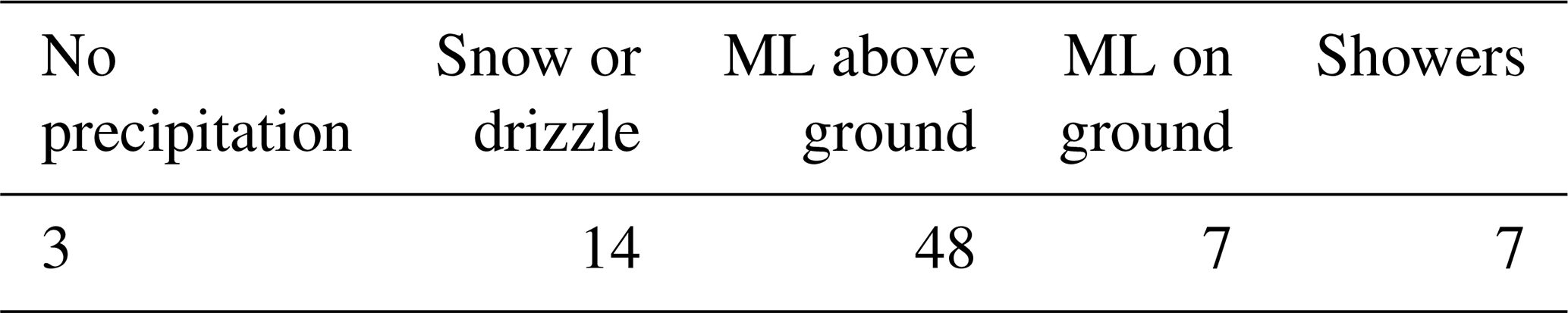
The ML can only be determined by eye for cases where the ML is fairly continuous in time; therefore, only events such as these were chosen to generate the “true” data. Many cases consist of fairly continuous rain at the surface and a well-developed ML above, but the training data also include MLs at the surface, cases with no ML due to snow or drizzle, and cases without any precipitation. Moreover, some cases with showers were included, where no ML was detected by eye and the desired output is “no ML”. In total, 79 intervals of 6 h were drawn, giving a total time of 474 h. An overview of the cases is given in Table 1. Within one interval, there can be more than one situation. In many cases, precipitation starts or stops; thus, the cases were classified on the basis of the most significant characteristic (e.g., “ML above ground” even if there was no precipitation for half the time).

Table 1 Overview of the training cases of 6 h intervals.

2.3 Neural network (NN)

NNs are modeled on the human brain. The idea is to connect individual artificial neurons and train them for a specific task. A neuron receives input data, combines the weighted input, and gives an output according to an activation function. The weights determine the importance of the input data, and the activation function determines the level of activity of the neuron. The output value is only transmitted if a threshold is exceeded. In a simple NN, such as the one used here, the neurons are arranged into an input and an output layer, with optional hidden layers in between, and the data only move forward through the NN. Each neuron is connected to all neurons in the previous and following layer. The connections between the neurons have a weight, which is random at the beginning and is adjusted during the training process to give the desired output. The training process is performed by providing the NN with data multiple times. Each time, the output of the NN is compared to the desired output, an error is calculated, and the weights are slightly adjusted to minimize the error. Once the NN is trained, it is evaluated using previously unseen data.

As input data, profiles of both ZEA and VEL proved to be the best choice. The combination of these two variables also produced the best results in Pfaff et al. (2014). Before using these profiles within the NN in this study, they needed to be prepared. First, the data were interpolated to a vertical resolution of 25 m, and aliasing of VEL was corrected. Moreover, where ZEA values fell below a threshold of −5 dBZ, ZEA and VEL were considered to be invalid. Because the NN is not able to process missing values, they were set to 0 for VEL and to −10 for ZEA. As the NN needs the values of the input to roughly range between zero and one, ZEA and VEL were scaled accordingly. To use the fact that the height of the ML shows some persistence in time, profiles of ZEA and VEL from four previous time steps were also used as input. Those four profiles were not taken from the time steps directly before but were spaced apart by six time steps in order to be able to “see” farther into the past without having to use all 24 profiles. To account for the fact that most MLs in the training dataset are located roughly in the middle of the profiles and to increase the volume of training data, the profiles were then subdivided. From each profile, the bottom 64 heights were taken as one sub-profile. The interval of 64 heights was then shifted by one height, and these 64 heights were taken as another sub-profile. This procedure was continued to the top 64 heights, resulting in 65 sub-profiles. This improved the prediction of MLs at the very bottom and top of the profiles. This whole preprocessing of the data resulted in an input array consisting of sub-profiles of multiple time steps of both ZEA and VEL, yielding $\mathrm{2}\times \mathrm{65}\times \mathrm{64}\times \mathrm{4}=\mathrm{33}\mathrm{280}$ values for each measurement time step of the MRR.

The NN used here is a feed-forward NN with two hidden layers. Each hidden layer has 64 neurons, and the learning rate at the beginning is 0.002. The “scikit-learn” Python library (Pedregosa et al., 2011) was used to develop the NN. Due to the large amount of training data, it was impractical to load all of the data into memory at once; thus, the order of the data and how often the individual datasets were used in training was determined manually. To be able to determine the performance of the NN during training, validation data were used. The training procedure of the NN began with iterating through all 6 h intervals of the training dataset once, successively in a random order. After each 6 h interval, the performance of the NN was determined with the validation data, and the mean square error (MSE) between the prediction and the “true” ML was calculated. For the calculation of the MSE, the prediction was slightly tweaked for false positive values to nudge the NN toward a conservative prediction. After one epoch, the mean MSE was calculated, and all 6 h intervals with an MSE larger than the mean MSE were not used for training in the following epochs. This means that the amount of training data decreases for each epoch until there are no more data left, denoting the end of the training. After each epoch, the learning rate was divided by 2, and the remaining data were again shuffled. If the mean MSE of one epoch was worse than that of the epoch before, that epoch was not used for training.

The validation data consisted of seven 6 h intervals, chosen to represent different situations such as an ML above the ground, an ML on the ground, a case with showers, and a case with snow. The common method of splitting all data randomly into training and validation data seemed impractical here, because it was important to cover many different meteorological situations within the validation set to ensure that the NN can handle them all well. Picking the validation data randomly would either result in not covering different situations or the random picking would have to be applied to individual profiles instead of 6 h intervals. However, this was impractical due to memory constraints and turned out to be unnecessary.

To ensure that the NN was not overfitted to the validation data, the rest of the measurement data, for which no “truth” was created, were used as test data. As the NN should handle all possible situations, the performance of the NN was assessed visually for the test data. The NN was adjusted, and the training process was repeated until the visual inspection showed a satisfactory result (see also Sect. 3).

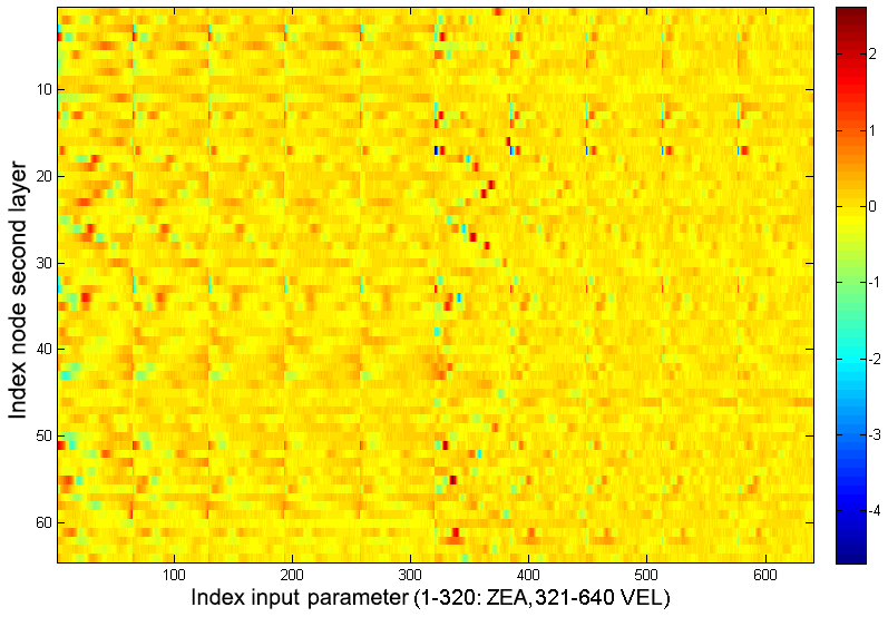
The trained NN consists of a number of weights. Figure 2 visualizes these weights for the input layer. The x axis shows the index of the input parameters, with indices 1–320 corresponding to the five sets of 64 heights of attenuated equivalent reflectivity and indices 321–640 corresponding to the fall velocity inputs; the y axis represents the index of the nodes of the second layer; and the colors denote the value of the weight. Figure 3 highlights the weights used to calculate the input for second-layer node 22 which are applied to the fall velocity. The sine-wave-like structure functions similarly to a gradient approximation, showing that the NN extracted the importance of the fall velocity gradient from the training data. The maximum and minimum of this structure correspond to heights 175 m apart, which aligns well with the expected width of the ML. The amplitude of the weights decreases with time, showing that the NN assigns higher importance to more recent velocity values and lesser importance to values that are farther in the past. Similar structures can be found for different second-layer nodes but at different heights, demonstrating that the NN searches for gradients in the fall velocity.

Figure 2 Neural network input layer weights.

Figure 3 Fall velocity weights for node 22 of the input layer.

After the training was complete, situations occurred in which an ML was incorrectly detected. Many of these situations had similar characteristics: they were situations with a high ML and an incorrectly detected second ML near the surface. Furthermore, sometimes the upper edge of valid MRR data was wrongly taken as an ML. Therefore, a post-processing step was included to remove the incorrect detections in these specific cases, based on fixed thresholds of the RR and signal-to-noise ratio. In addition, MLs that lasted less than six time steps were removed to avoid short-term clutter, and MLs with a confidence of less than 0.2 were set to 0.

3 Results

This section describes the performance of the fully trained NN, starting with a straightforward case of a well-developed continuous ML. Then, more complex cases are shown to give an overview of the range of possible situations and to show how the NN is able to handle these situations. Sensitivity studies of vertical and temporal resolutions and comparisons with an ML detected by weather radars, with radiosonde data, and with a cloud radar are also shown.

3.1 Performance of the NN

An example of the performance of the NN is given in Fig. 4 for a well-developed ML. In the time period shown, there is a continuous ML at about 1900 m and rain below this level. The output of the NN is shown in the range between zero and one, indicating the uncertainty with which the NN detects the ML. Values close to one indicate a high confidence in the existence of an ML. The ML detected by the NN is fairly broad. This is due to the training data, in which the ML starts at the top with completely frozen particles and ends only when all particles are liquid. This means that the NN will also give broad MLs. The NN could also have been trained with one ML height, such as the middle of the ML height; this is a design choice. The thickness of the ML is influenced by the precipitation intensity in the training data, and the ML thickness detected by the NN in the test data is also influenced by the precipitation intensity. This behavior has previously been observed in studies such as Klaassen (1988).

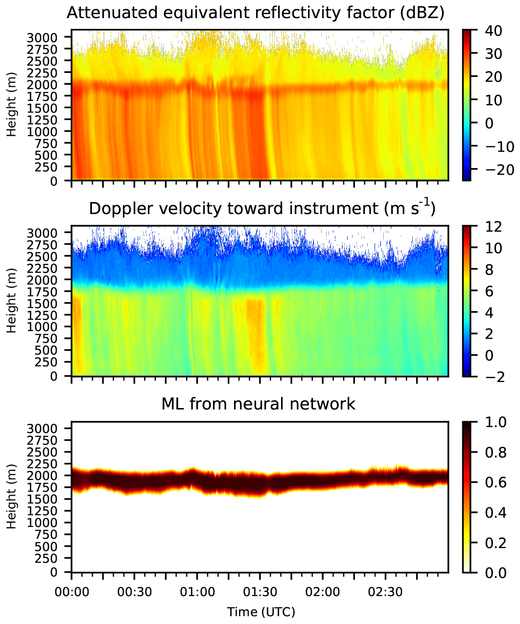
Figure 4 ZEA, VEL, and ML detected by the NN for Hohenpeißenberg on 13 June 2018 from 00:00 to 03:00 UTC.

Although the performance of the NN in the situation shown in Fig. 4 is obviously good, the NN needs to be validated for many different situations if it is to be used operationally. However, calculating a metric to quantify the error is difficult, as common metrics such as the mean square error or probability of detection all need to know the expected outcome. Section 2.2 describes the procedure with which “true” data were generated, which were needed for training the NN. We wanted to use as much data as possible for the training process, because the performance of the NN depends on the amount of training data. Therefore, most of the data for which a “truth” was generated were used to train the NN, and the rest of the “true” data were used for validation. During training of the NN, it was constantly tested against a validation dataset and the mean square error was calculated (see Sect. 2.3), which determined when the training was complete. For testing the NN, no “true” data were used, as the creation of “true” data is time-consuming and only possible for situations where the eye can easily identify an ML. Moreover, we wanted the NN to be conservative, meaning that a false negative is considered less severe than a false positive. Therefore, during the development of the NN, its performance was visually inspected and a low MSE was not automatically considered to be a good result. The final evaluation of the NN was conducted by plotting the output of the NN as well as the time series of the profiles of ZEA, VEL, and other variables. All of the available 261 d of data were then visually inspected and evaluated. In the following, a few cases are shown that are exemplary of the performance of the NN under different weather conditions.

Figure 5 shows a case without an ML. The temperature on the ground is below 0 ^∘C, and the precipitation is snow throughout the measurement range. ZEA has no maximum, and VEL shows no acceleration. The NN correctly detects the absence of an ML.

Figure 5 Same as Fig. 4 but for Hohenpeißenberg on 18 November 2018 from 18:00 to 21:00 UTC.

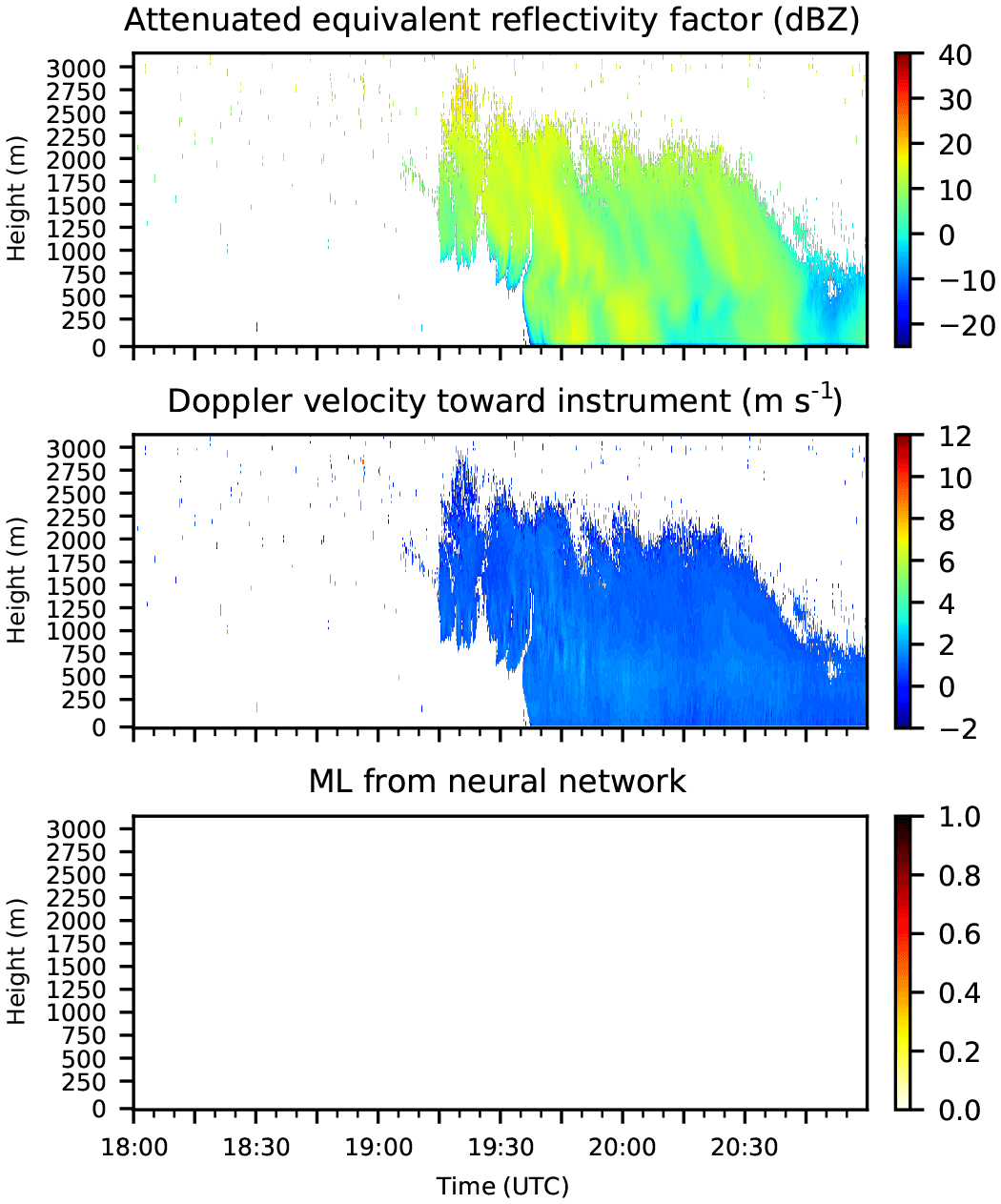
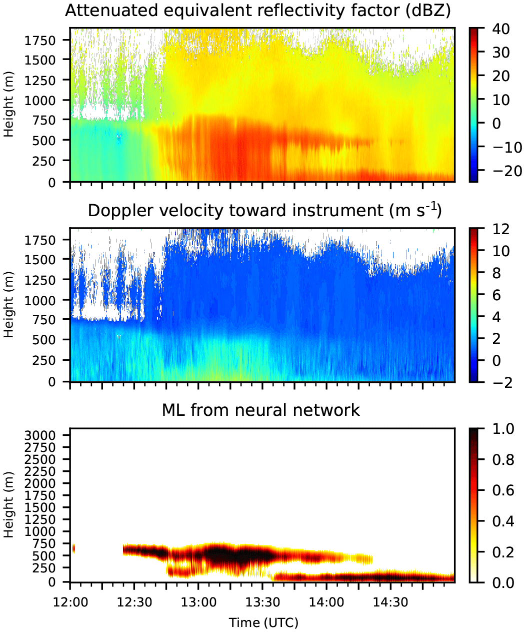
Figure 6 shows a case where the ML lifts from the ground. Surface observations measured a temperature (at a height of 2 m) of around 1.5 ^∘C at 00:00 UTC, increasing to about 3.5 ^∘C at 03:00 UTC, and the precipitation at the surface turned from sleet to rain. In the beginning, the snow had started to melt, but the melting process had not finished above ground. With increasing temperature, the melting began higher up and was complete before the precipitation hit the ground.

Figure 6 Same as Fig. 4 but for Hamburg on 14 December 2017 from 00:00 to 03:00 UTC.

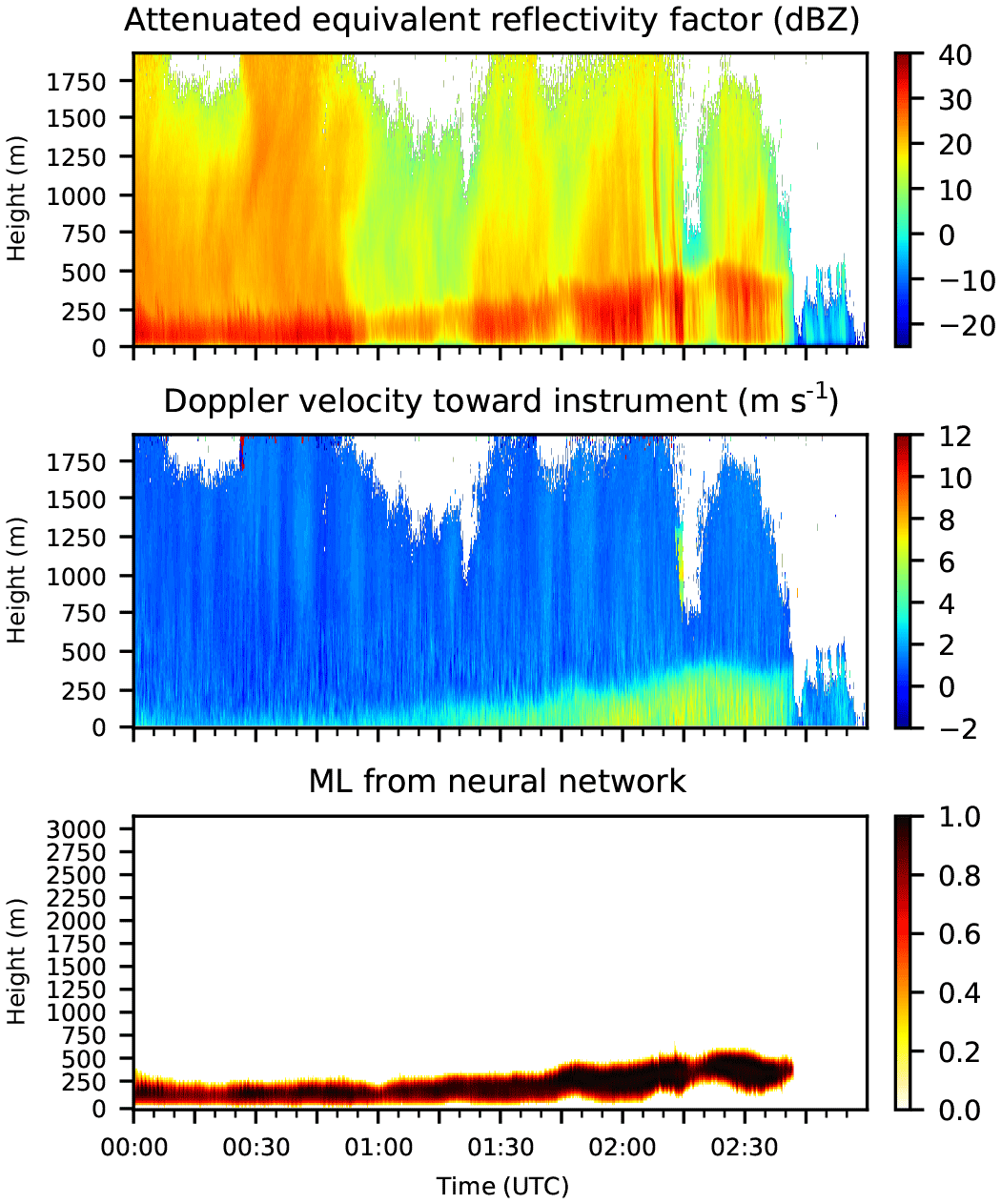
Figure 7 shows a convective case with showers. In these situations, the ML is not continuous in space and time as it is in a case with a homogeneous cloud layer and stratiform rain. During these short rain events, the measured profiles of vertical velocity and reflectivity are distorted because the falling rain is skewed; thus, the NN is not given profiles in which the melting is fully contained. The detection of an ML by eye is consequently difficult or even impossible in such cases; accordingly, the NN has difficulties dealing with these situations. During the training process, the NN was tuned to detect as little as possible in the abovementioned situations, but it was not possible to train the NN not to detect anything without impeding its abilities in other cases. Therefore, the NN has the most problems with convective cases.

Figure 7 Same as Fig. 4 but for Hohenpeißenberg on 31 August 2017 from 12:00 to 15:00 UTC.

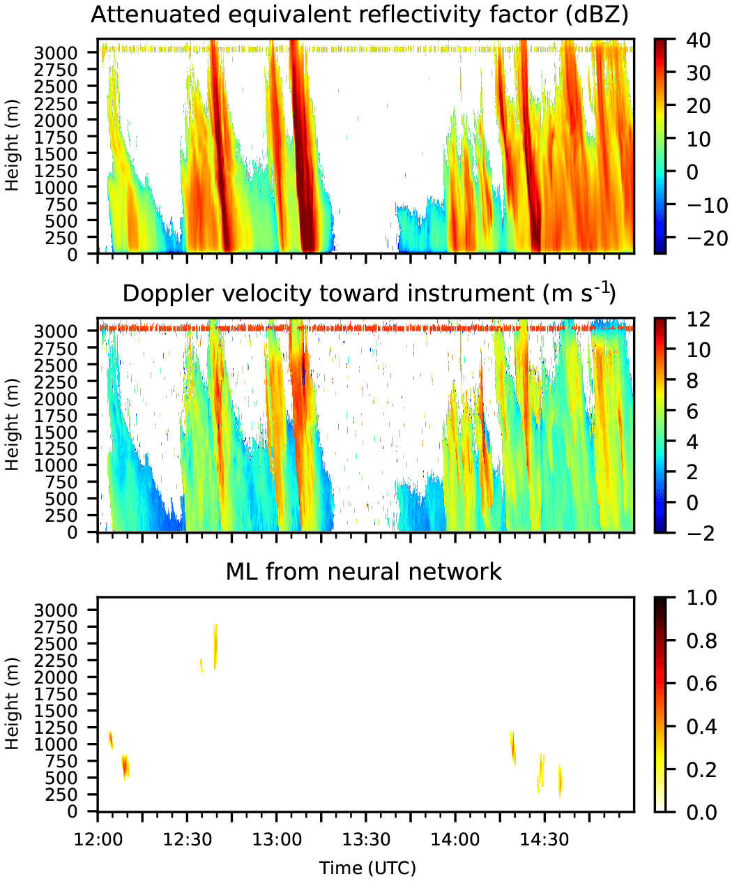
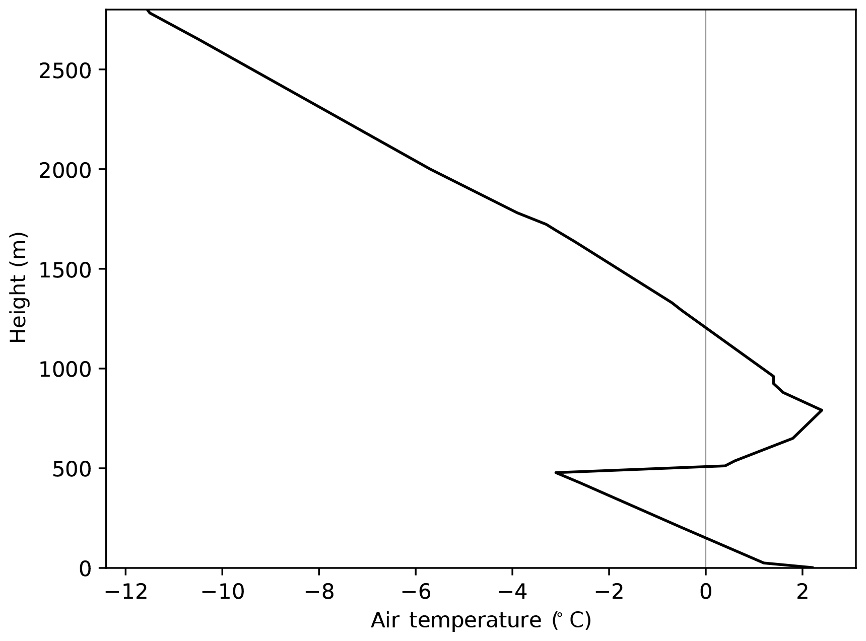
In our dataset we found two cases where two concurrent MLs were clearly visible, one of which is shown in Fig. 8. At Greifswald at 12:00 UTC, the radiosonde measured two layers with temperatures above freezing, one freezing layer in between, and freezing temperatures above (Fig. 9). The two MLs in the radar data are visible to the eye, especially in the reflectivity data. The time difference in the occurrence of the two ML in the radiosonde and radar data can be sourced to the different locations, which are about 100 km apart. The NN also observes the two MLs, despite the fact that there were no such cases in the training dataset. This is a sign that the NN is able to generalize.

Figure 8 Same as Fig. 4 but for Hamburg on 31 March 2018 from 12:00 to 15:00 UTC.

Figure 9 Radiosonde from Greifswald on 31 March 2018 at 12:00 UTC.

3.2 Sensitivity studies

For the NN to work operationally, it must be ensured that it can handle various MRR operation parameter settings. Therefore, four 6 h intervals with precipitation from an MRR located in Elmshorn with a vertical resolution of 50 m and ten 6 h intervals with a resolution of 100 m were tested. As all data are first interpolated to a resolution of 25 m and the NN expects 128 height levels, no ML can be detected above 3200 m. Because the ML heights in the data from Elmshorn are below this height, the NN was able to detect the ML well, proving that it can handle data with various vertical resolutions up to 100 m. For even coarser vertical resolutions, the NN might have trouble detecting an ML, as the resolution might then be of the same order as or even larger than the vertical extent of the ML.

The sensitivity of the NN to the temporal resolution of the data was also tested. The NN was trained with a temporal resolution of 10 s and with profiles of five different times that were each 1 min apart from the next profile. As the NN should work for different MRR operational settings, it should also give good results when an MRR is operated with a larger averaging interval. Therefore, part of the test dataset (20 d) was averaged over 30 s and 1 min, respectively, and the NN was again given five profiles that were each 1 min apart from the next. The output of the NN was then visually inspected. Only averages up to 1 min were tested because MRRs are seldom operated with longer averaging intervals. The difference between the various averaging intervals are small (not shown). In general, for a longer temporal average, the detected ML gets smoother. In some cases, the NN with a larger averaging interval incorrectly detects an ML with a low probability for short periods of time (“clutter”). Moreover, the edges of the ML are less clearly defined, which is manifested by slightly larger tails with a low probability of an ML being detected. However, in some cases there are small gaps in the detected ML for the short averaging interval of 10 s where the ML is detected in some time steps but not in others. This results in small fragments of a correctly detected ML which might, in addition, be filtered out by the criterion that MLs lasting less than six time steps are removed. For larger averaging intervals, these gaps are sometimes filled due to the smoothing of the data. The described differences only appear in cases where the detection of an ML is somewhat difficult due to factors such as showers, whereas differences between the different temporal averages are hardly discernible for most cases. Therefore, we conclude that the NN is able to handle different temporal resolutions of MRR data up to a resolution of 1 min.

3.3 Comparison to C-band radar

The ML height detected by the NN was compared to the ML height detected by C-band radars deployed by the German Weather Service (DWD). The DWD is in the process of developing an ML detection algorithm for the operational weather radars in Germany, which is supported by the COSMO-D2 numerical model. For the two MRR instrument locations where most of the data used in this study were collected, the ML was compared to the ML detected by the surrounding C-band radars. For the MRR at Hamburg airport, the surrounding weather radars are located at Boostedt, Rostock, and Hannover. For Hohenpeißenberg, they are located at Türkheim, Isen, and Memmingen. Data are available until June 2018. For 35 (18) of the 90 (84) d during which the MRR detected precipitation in Hamburg (Hohenpeißenberg), at least one weather radar in the vicinity of the MRR detected an ML at the location of an MRR. Many cases were detected by the MRR but not by the weather radars. This is primarily due to the fact that the weather radars are too far away from the MRR.

Figure 10 shows an example of the MRR data with the ML detected by the algorithm using weather radars and model data overlain as dots on the output of the NN. The C-band radars do a volumetric scan every 5 min; therefore, the temporal resolution of the detected ML is much coarser than that of the MRR. In the case shown, the different weather radars disagree on the exact height of the ML, possibly because the weather radars measure with a low elevation angle and are located between 40 and 90 km away from the MRR; therefore, the vertical resolution of the C-band radar over the MRR is around 700 m for the closest radar and around 1500 m for the farthest radar. Furthermore, the coarser spatial resolution could explain the differences from the MRR, as the scanned volume might be different. The MRR seems to be much better suited to detecting the ML height at one location; thus, the information from the MRR might aid the detection algorithm of the weather radars.

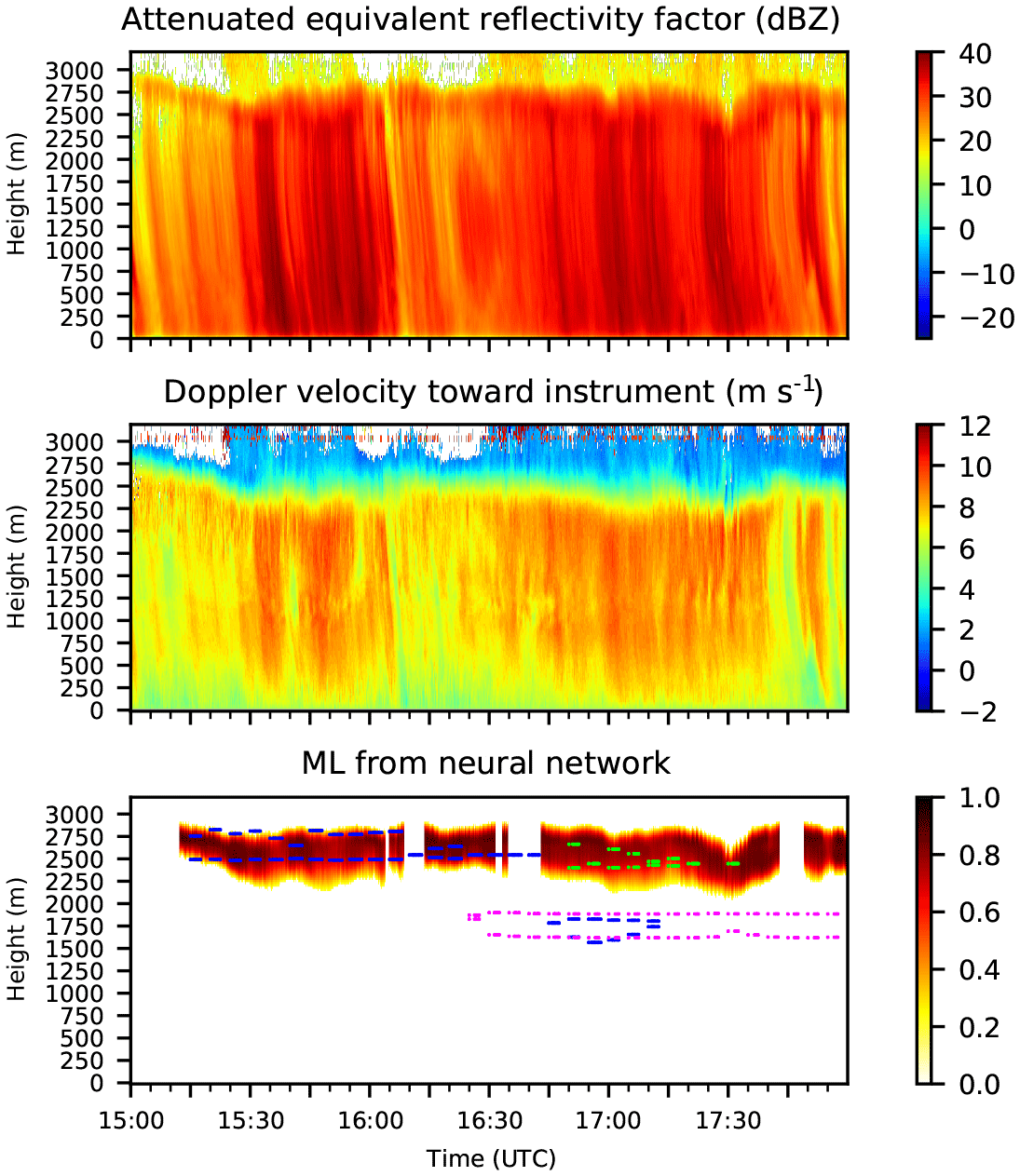
Figure 10 ZEA, VEL, and ML detected by the NN for Hohenpeißenberg on 10 August 2017 from 15:00 to 18:00 UTC. The dashed lines indicate the top and bottom of the ML heights detected by three weather radars: green represents Isen, blue represents Memmingen, and pink represents Türkheim.

3.4 Comparison of the ML height to radiosondes

The ability of the NN to determine the ML height has mostly been assessed by visual comparison with the other data measured by the MRR (see Sect. 3.1). As explained in Sect. 2.2, it is difficult to find other sources of the ML height with which a meaningful comparison can be made. At Hohenpeißenberg, radiosondes are launched about twice a week to measure ozone. These radiosondes also measure temperature; thus, a comparison can be made between the height of the freezing level of the radiosonde and the top height of the ML detected by the NN, as the frozen particles should start to melt at the 0 ^∘C temperature level. Such a comparison has limitations, because precipitation must be detected by the MRR within a short time period of the radiosonde launch time. Moreover, the weather conditions must be fairly constant so that a sudden change in ML height is unlikely and it can be assumed that the ML height detected by the MRR can be compared to the 0 ^∘C height of the radiosonde. When sorting through the available radiosonde data, cases were rejected when it was clear from MRR data that the precipitation and, therefore, the ML height might be changing too quickly or the duration of the precipitation was less than 2 min. From all available data from Hohenpeißenberg, 18 cases were found for which a fairly reasonable comparison can be made. Figure 11 shows a comparison between the freezing level of the radiosonde and the top height of the ML determined by the NN. As the time difference between the detected ML by the NN and the measurement of the radiosonde is up to about 5 h and the radiosonde drifts horizontally as it rises, the value of this comparison is limited. Nevertheless, there is a good overall agreement between the radiosondes and the NN almost independent of the time difference between the ML measured by the NN and the radiosonde. The largest difference between the ML top and freezing level is about 320 m for a case where the time difference between both measurements is about 3.5 h. In four cases, the radiosonde measured negative temperatures at the surface and the NN correctly detected no ML (blue circles at height 0 m in Fig. 11).

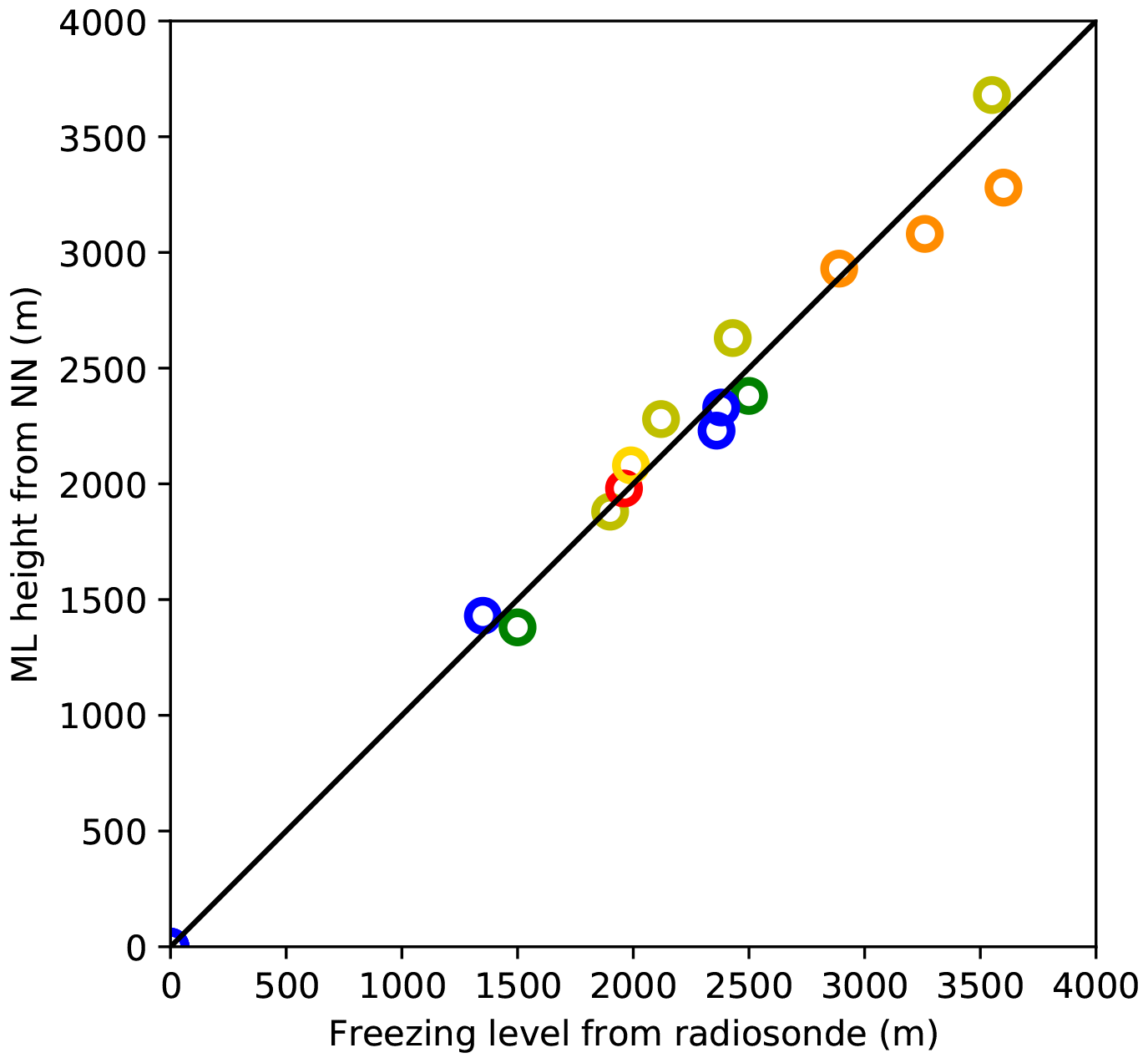
Figure 11 Comparison between the ML height determined by the NN and the freezing level from the radiosonde for Hohenpeißenberg. The colors denote the time difference between the two heights: no difference (blue), 0–1 h (green), 1–2 h (olive green), 2–3 h (yellow), 3–4 h (orange), and 4–5 h (red).

3.5 Comparison of the ML height to the cloud radar

For 4 additional days in December 2018 and January 2019, a comparison between the ML detected by the NN and a cloud radar (MIRA-35 by METEK, 30 m vertical resolution) was made. The cloud radar determines an ML height to identify plankton. The ML is determined from the linear depolarization ratio (LDR) in the vicinity of the ML taken from a database (METAR-data, radio soundings, or model data). Figure 12 shows an example of this comparison. The background shows ZEA measured by the MRR for reference. The gray area denotes the ML detected by the NN, and the blue line is the ML detected by the cloud radar. The ML from the NN is fairly broad and encompasses the maximum of the reflectivity, as described in the previous sections. The ML from the cloud radar mostly follows the bottom boundary of the ML detected by the NN. This is caused by the way that the ML is determined by the cloud radar. The LDR is sensitive where the particles are already mostly melted, whereas the NN considers the whole process of melting. Considering these differences in the purpose and determination of the ML, the agreement between both instruments is very good.

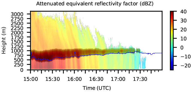
Figure 12 Comparison between the ML height determined by the NN and by a cloud radar for Elmshorn on 22 December 2018 from 15:00 to 18:00 UTC. The colors in the background show the ZEA from the MRR, the gray shading denotes the area where the NN detected an ML, and the blue line is the ML detected by a cloud radar.

4 Discussion and conclusion

We have developed an NN to detect the ML from MRR data operationally. The available data encompass measurements from all seasons and from two MRRs at two locations in Germany: an isolated mountain in the very south of Germany and a location on the North German Plain. Using this dataset, the NN was tested extensively.

Overall, the NN was able to detect the correct ML height well. Some weather conditions were more difficult for the NN to handle than other situations. Cases where an ML was located well above the ground and was fairly continuous in time and space were the easiest situations, and the NN handled them best. The most frequent situations in which the NN was not able to capture the ML height well were those with discontinuous precipitation associated with convection. In these cases, the human eye could also hardly detect the ML height in the measurement data. These situations are more frequent in summer due to stronger and more frequent convection in this season. Moreover, in some situations with snowfall, the NN detected clutter near the ground (incorrectly detected MLs with a low probability and a small vertical and temporal extent), which is not covered by the suppression of clutter in the post-processing. More uncommon situations where the NN was sometimes unable to correctly detect an ML were situations when (i) there was strong horizontal wind, (ii) the signal directly below the ML was weak, (iii) there were disturbances in the signal, or (iv) the dealiasing of the fall velocity failed. Horizontal wind leads to slanted structures of precipitation, which violates the assumption of the NN that an ML can be derived from characteristics within one vertical profile. Although aliasing of the fall velocity is corrected, this algorithm is not able to handle rare situations where the fall velocity is shifted by large amounts due to strong convection.

To ensure that the NN is able to handle different averaging intervals of the input data and different settings of the vertical resolution of the MRR, sensitivity studies were carried out. These tests showed that the NN is able to handle temporal averaging up to 1 min and different vertical resolutions of up to 100 m. Furthermore, a comparison to radiosonde data was made at Hohenpeißenberg where one MRR was located and radiosondes were launched. Although there were only a few simultaneous ML observations, the agreement with respect to the ML height was very good. In addition, the detected ML is consistent with measurements from a cloud radar.

The NN presented here was designed to be used operationally and to handle different weather conditions and MRR settings. Some decisions were made during development concerning the design of the NN and the desired output. One such choice was the broad width of the detected ML, encompassing the whole process of melting. While tuning the NN, a balance was sought between too many false positive detections and too many false negative detections. For some applications, few false positives might be more beneficial, whereas few false negatives might be more important for other applications. The decisions made for this NN were aimed to ensure validity over a broad range of applications.

This study showed that an NN approach is well suited for detecting the pattern of the ML from radar data. Although we used the MRR, in principle this approach can be used by other types of radars as well. In contrast to deterministic methods (e.g., Fabry and Zawadzki, 1995; White et al., 2002; Cha et al., 2009; Perry et al., 2017), the NN is able to detect uncommon MLs such as MLs on the ground or two MLs at once, and it does not need to be given thresholds or the shape of a profile with an ML in advance. A disadvantage of this method is that an NN lacks a physical basis and is, thus, not suited to study the physics within the ML. In principle, the time resolution of our approach can be as high as the time resolution of the measuring radar, allowing the possibility to detect fast changes in the ML height, which can be important for applications such as those at airports. Post-processing can include time-averaging and filtering of short ML occurrences if a false positive detection is deemed worse than a false negative detection.

Future work could include using data from other climatic regions. Also, the preparation of the data, such as the dealiasing of the fall velocity, or the post-processing of the NN could be improved. The chosen algorithms for data preparation and post-processing are designed to be fast enough for real-time use within an MRR; therefore, their complexity was limited. Extending these algorithms might improve the performance of the NN.

Possible applications for the NN presented are, for example, airports, where reliable ML data could add important information to help detect the danger of icing. Local data can also be used as supporting information to improve the quality of spatial ML data as provided by weather radars or numerical models.