the Creative Commons Attribution 4.0 License.
the Creative Commons Attribution 4.0 License.
 | 16 Mar 2021
LiSBOA (LiDAR Statistical Barnes Objective Analysis) for optimal design of lidar scans and retrieval of wind statistics – Part 1: Theoretical framework
Stefano Letizia
Lu Zhan
Giacomo Valerio Iungo
A LiDAR Statistical Barnes Objective Analysis (LiSBOA) for the optimal design of lidar scans and retrieval of the velocity statistical moments is proposed. LiSBOA represents an adaptation of the classical Barnes scheme for the statistical analysis of unstructured experimental data in N-dimensional space, and it is a suitable technique for the evaluation over a structured Cartesian grid of the statistics of scalar fields sampled through scanning lidars. LiSBOA is validated and characterized via a Monte Carlo approach applied to a synthetic velocity field. This revisited theoretical framework for the Barnes objective analysis enables the formulation of guidelines for the optimal design of lidar experiments and efficient application of LiSBOA for the postprocessing of lidar measurements. The optimal design of lidar scans is formulated as a two-cost-function optimization problem, including the minimization of the percentage of the measurement volume not sampled with adequate spatial resolution and the minimization of the error on the mean of the velocity field. The optimal design of the lidar scans also guides the selection of the smoothing parameter and the total number of iterations to use for the Barnes scheme. LiSBOA is assessed against a numerical data set generated using the virtual lidar technique applied to the data obtained from a large eddy simulation (LES). The optimal sampling parameters for a scanning Doppler pulsed wind lidar are retrieved through LiSBOA, and then the estimated statistics are compared with those of the original LES data set, showing a maximum error of about 4 % for both mean velocity and turbulence intensity.
- Article
(10930 KB) - Full-text XML
- Companion paper
- BibTeX
- EndNote


Reliable measurements of the wind velocity vector field are essential for understanding the complex nature of atmospheric turbulence and providing valuable data sets for the validation of theoretical and numerical models. However, field measurements of wind speed are typically characterized by large uncertainties due to the generally unknown and uncontrollable boundary conditions (Braham, 1979), the broad range of timescales and length scales (Cushman-Roisin and Beckers, 1990a), and the complexity of the physics involved (Stull, 1988). Furthermore, the large measurement volume, which typically extends throughout the height of the atmospheric boundary layer, imposes on the experimentalists the selection of the sampling parameters as a trade-off between spatial and temporal resolutions.
Wind speed has been traditionally measured through local sensors, such as mechanical, sonic, and hot-wire anemometers (Liu et al., 2019; Kunkel and Marusic, 2006). Besides their simplicity, mechanical anemometers are affected by errors due to the flow distortion of the supporting structures, drawbacks under harsh weather conditions (Mortensen, 1994), and overspeeding (Busch and Kristensen, 1976). Furthermore, their relatively slow response results in a limited range of the measurable time–length scales, which makes them unsuitable, for instance, for measuring the turbulent flow around urban areas (Pardyjak and Stoll, 2017). Sonic anemometers can measure the three velocity components, with frequencies up to 100 Hz (Cuerva and Sanz-Andrés, 2000), in a probing volume of the order of 10−4 m3, yet measurements might be still affected by the wakes generated by the supporting structures, such as met towers and struts, and they are sensitive to temperature variations (Mortensen, 1994). Hot-wire anemometers, although they provide a full characterization of the energy spectrum, require a complicated calibration (Kunkel and Marusic, 2006) and are extremely fragile (Wheeler and Ganji, 2010a). Furthermore, traditional, single-point sensors are unable to provide an adequate characterization of the spatial gradients of the wind velocity vector, which is particularly significant in the vertical direction (Cushman-Roisin and Beckers, 1990b). To overcome this issue, several anemometers arranged in arrays, and supported by meteorological masts, have been deployed in several field campaigns (Haugen et al., 1971; Bradley, 1983; Taylor and Teunissen, 1987; Emeis et al., 1995; Pahlow et al., 2001; Berg et al., 2011; Kunkel and Marusic, 2006).
In the last few decades, remote sensing instruments have been increasingly utilized to probe the atmospheric boundary layer (Debnath et al., 2017a, b), and nowadays they represent a more cost-effective and flexible alternative to meteorological towers (Newsom et al., 2017). In particular, in the realm of remote sensing anemometry, Doppler wind light detection and ranging (lidar) systems underwent a rapid development due to the significant advancement in eye-safe laser technology (Emeis, 2010). Wind lidars have been heavily employed in wind energy (Bingöl et al., 2010; Aitken and Lundquist, 2014; Trujillo et al., 2011; Iungo et al., 2013b; Machefaux et al., 2016; Garcia et al., 2017; El-Asha et al., 2017; Bromm et al., 2018; Zhan et al., 2019, 2020), airport monitoring (Köpp et al., 2005; Tang et al., 2011; Holzäpfel et al., 2016; Thobois et al., 2019), micro-meteorology (Gal-Chen et al., 1992; Banakh et al., 1999; Banta et al., 2006; Mann et al., 2010; Muñoz-Esparza et al., 2012; Rajewski et al., 2013; Schween et al., 2014), urban wind research (Davies et al., 2007; Newsom et al., 2008; Xia et al., 2008; Kongara et al., 2012; Huang et al., 2017; Halios and Barlow, 2018), and studies of terrain-induced effects (Bingöl, 2009; Krishnamurthy et al., 2013; Kim et al., 2016; Pauscher et al., 2016; Risan et al., 2018; Fernando et al., 2019; Bell et al., 2020).
Besides the mentioned capabilities, lidars present some important limitations, such as reduced range in adverse weather conditions (precipitation, heavy rain, fog, low clouds, or low aerosol concentration; Liu et al., 2019; Mann et al., 2018) and a limited spatiotemporal resolution of this instrument, namely about 20 m in the radial direction and about 10 Hz in sampling frequency. These technical specifications, associated with the nonstationary wind conditions typically encountered for field experiments, pose major challenges in the application of wind lidars for the statistical analysis of turbulent atmospheric flows.
In the realm of wind energy, early lidar measurements were limited to the qualitative analysis of snapshots of the line-of-sight (LOS) velocity, i.e., the velocity component parallel to the laser beam (Käsler et al., 2010; Clive et al., 2011). Fitting of the wake velocity deficit was also successfully exploited for the extraction of quantitative information about wake evolution from lidar measurements (Aitken and Lundquist, 2014; Wang and Barthelmie, 2015; Kumer et al., 2015; Trujillo et al., 2016; Bodini et al., 2017). To characterize velocity fields with higher statistical significance, the time averages of several lidar scans were calculated for periods with reasonably steady inflow conditions (Iungo and Porté-Agel, 2014; Machefaux et al., 2015; Van Dooren et al., 2016). In the case of data collected under different wind and atmospheric conditions, clustering and bin-averaging of lidar data were carried out (Machefaux et al., 2016; Garcia et al., 2017; Bromm et al., 2018; Zhan et al., 2019, 2020). Finally, more advanced techniques for first-order statistical analysis, such as variational methods (Xia et al., 2008; Newsom and Banta, 2004), optimal interpolation (Xu and Gong, 2002; Kongara et al., 2012), least squares methods (Newsom et al., 2008), and Navier–Stokes solvers (Astrup et al., 2017; Sekar et al., 2018), were applied for the reconstruction of the velocity vector field from dual Doppler measurements.
Besides the mean field, the calculation of higher-order statistics from lidar data to investigate atmospheric turbulence is still an open problem. In this regard, Eberhard et al. (1989) re-adapted the postprocessing of the velocity azimuth display (VAD) scans (Lhermitte, 1969; Wilson, 1970; Kropfli, 1986) to estimate all the components of the Reynolds stress tensor by assuming horizontal homogeneity of the mean flow within the scanning volume, which can be a limiting constraint for measurements in complex terrains (Frisch, 1991; Bingöl, 2009). Range height indicator (RHI) scans were used to detect second-order statistics (Bonin et al., 2017), spectra, skewness, dissipation rate of the velocity field, and even heat flux (Gal-Chen et al., 1992). Recently, in the context of wind radar technology, but readily applicable to lidars as well, a promising method for the estimation of the instantaneous turbulence intensity (i.e., the ratio between standard deviation and mean of streamwise velocity), based on the Taylor hypothesis of frozen turbulence, was proposed by Duncan et al. (2019). More advanced techniques exploit additional information of turbulence carried by the spectrum of the backscattered lidar signal (Smalikho, 1995). However, this approach requires the availability of lidar raw data, which is not generally available for commercial lidars. For a review on turbulence statistical analyses through lidar measurements, the reader can refer to Sathe and Mann (2013). Another typical scanning strategy to obtain high-frequency lidar data consists of performing scans with fixed elevation and azimuthal angles of the laser beam while maximizing the sampling frequency (Mayor et al., 1997; O'Connor et al., 2010; Vakkari et al., 2015; Frehlich and Cornman, 2002; Debnath et al., 2017b; Choukulkar et al., 2017; Lundquist et al., 2017).
For remote sensing instruments, data are typically collected based on a spherical coordinate system, and then interpolated over a Cartesian reference frame oriented with the x axis in the mean wind direction. This interpolation can be a source of error (Fuertes Carbajo and Porté-Agel, 2018), especially if a linear interpolation method is used (Garcia et al., 2017; Carbajo Fuertes et al., 2018; Beck and Kühn, 2017; Astrup et al., 2017). Delaunay triangulation has also been widely adopted for coordinate transformation (Clive et al., 2011; Trujillo et al., 2011, 2016; Iungo and Porté-Agel, 2014; Machefaux et al., 2015), yet the accuracy has not been quantified in the case of nonuniformly distributed data. It is reasonable to weight the influence of the experimental points on their statistics according to the distance from the respective grid centroid, such as using uniform (Newsom et al., 2008), hyperbolic (Van Dooren et al., 2016), or Gaussian weights (Newsom et al., 2014; Wang and Barthelmie, 2015; Zhan et al., 2019). The use of distance-based Gaussian weights for the interpolation of scattered data over a Cartesian grid is at the base of the Barnes objective analysis (or Barnes scheme; Barnes, 1964), which has been systematically used in meteorology but only sporadically used for lidar data. It represents an iterative statistical ensemble procedure to reconstruct a scalar field arbitrarily sampled in space and is low-pass filtered with a cut-off wavelength that is a function of the parameters of the scheme.
The scope of this work is to define a methodology to postprocess scattered data of a turbulent velocity field measured through a scanning Doppler wind lidar (or eventually other remote sensing instruments) to calculate mean, standard deviation and even higher-order statistical moments on a Cartesian grid. The proposed methodology, referred to as the LiDAR Statistical Barnes Objective Analysis (LiSBOA), represents an adaptation of the classic Barnes scheme to N-dimensional domains, enabling applications for nonisotropic scalar fields through a coordinate transformation. A major point of novelty of LiSBOA is the estimation of wind velocity variance (and, eventually, higher-order statistics) from the residual field of the mean, which also provides adequate filtering of dispersive stresses due to data variability not connected with the turbulent motion. A criterion for the rejection of statistical data affected by aliasing, due to the undersampling of the spatial wavelengths under investigation, is formulated. LiSBOA is assessed against a synthetic scalar field to validate its theoretical response and the formulated error metric. Detailed guidelines for the optimal design of a lidar experiment and the effective reconstruction of the wind statistics are provided. The effectiveness of the proposed scheme in the identification of the optimal scanning parameters and retrieval of turbulence statistics is quantified using virtual lidar data.
It will be shown in the following that the revisited Barnes scheme offers several advantages compared to the above-cited techniques for lidar data analysis: (i) it allows one to explicitly select the cut-off wavenumber to filter out small-scale variability, while retaining relevant modes in the flow field; (ii) the distance-based weighting function provides smoother fields than linear interpolation or window average, while still being simpler and computationally inexpensive compared to more sophisticated techniques (e.g., optimal interpolation and variational methods); and (iii) it provides guidance for the optimal design of lidar scans to investigate specific wavelengths in the flow. On the other hand, the procedure requires estimates of input parameters for the flow under investigation and the lidar system used. In case these parameters cannot be obtained from existing literature or preliminary tests, a sensitivity study on the variability in the LiSBOA results to the input parameters can be carried out.
The remainder of the paper is organized as follows: in Sect. 2, the extension of the Barnes scheme theory to N-dimensional domains and higher-order statistical moments is presented. In Sect. 3, the theoretical response function of LiSBOA is validated against a synthetic case, while guidelines for proper use of the proposed algorithm and optimal scan design are provided in Sect. 4. In Sect. 5, the accuracy of LiSBOA is tested, using the virtual lidar technique. Challenges in the application of the methodology to field experimental data are then discussed in Sect. 6. Finally, concluding remarks are provided in Sect. 7.
The Barnes scheme was originally conceived as an iterative algorithm aiming to interpolate a set of sparse data over a Cartesian grid (Barnes, 1964), and it was inspired by the successive correction scheme by Cressman (1959). The first iteration of the algorithm calculates a weighted space-averaged field, g0, over a Cartesian grid from the sampled scalar field, f. The mean field is iteratively modified by adding contributions to recover features characterized by shorter wavelengths, which are inevitably damped by the initial averaging process. In this work, we adopt the most classical form of the Barnes scheme as follows:
where is the average field at the ith grid node with coordinates ri (bold symbols indicate vectorial quantities) for the mth iteration, fj is the scalar field sampled at the location rj, and ϕ represents the linear interpolation operator from the Cartesian grid to the sample location. The weights for the sample acquired at the location rj and for the calculation of the statistics of f at the grid node, with coordinates ri, wij, are defined as follows:
where σ is referred to as the smoothing parameter, and indicates Euclidean norm. For practical reasons, the summations over j are performed over the neighboring points included in a ball with a finite radius Rmax (also called the radius of influence) and centered at the ith grid point. In this work, following Barnes (1964), we select Rmax=3σ, which encompasses 99.7 % and 97 % of the volume of the weighting function in 2D and 3D, respectively.
In the literature, there is a lack of consensus regarding the selection of the total number of iterations (Barnes, 1964; Achtemeier, 1989; Smith and Leslie, 1984; Seaman, 1989) and the smoothing parameter (Barnes, 1994a; Caracena, 1987; Pauley and Wu, 1990). A reduction of the smoothing parameter, σ, as a function of the iteration, m, was originally proposed by Barnes (1973); however, this approach turned out to be detrimental in terms of noise suppression (Barnes, 1994c).
In the frequency domain, the Barnes objective analysis is tractable as a low-pass filter applied to a scalar field, f, with a response as a function of the spatial wavelength, depending on the smoothing parameter, σ, and the number of iterations, m. This feature has been exploited in meteorology to separate small-scale from mesoscale motions (Doswell, 1977; Maddox, 1980; Gomis and Alonso, 1990). The spectral behavior of the Barnes scheme has been traditionally characterized by calculating the so-called continuous response at the mth iteration, Dm(k), with k being the wavenumber vector. Dm(k) is defined as the ratio between the amplitude of the Fourier mode eik⋅x (with ) for the reconstructed field, gm, to its amplitude in the input field, f, in the limit of a continuous distribution of samples and an infinite domain. The analytical expression for the continuous response was provided by Barnes (1964) and Pauley and Wu (1990) for 1D and 2D domains, respectively, while, in the context of LiSBOA, it is extended to N dimensions to enhance its applicability. Furthermore, besides the spatial variability of f, the temporal coordinate, t, is introduced to determine the response of the statistical moments of f.
We consider a continuous scalar field, f(x,t), which is defined over an N-dimensional domain, x. It is further assumed that the field f is ergodic in time. In practice, ergodic data can be obtained by selecting samples collected for a temporal window exhibiting stationary boundary conditions or, more generally, through a cluster analysis of discontinuous data (Machefaux et al., 2016; Bromm et al., 2018; Iungo et al., 2018; Zhan et al., 2019, 2020). By adopting the approach proposed by Pauley and Wu (1990), and by taking advantage of the isotropy of the Gaussian weights (Eq. 2), we can define the LiSBOA operator at the 0th iteration as follows:
where t1 and t2 are initial and final time. The term within the square brackets represents the mean of f over the considered sampling interval [t1,t2], which is indicated as . Moreover, to reconstruct a generic qth central statistical moment of the scalar field, f, it is sufficient to apply the LiSBOA operator of Eq. (3) to the fluctuations over to the qth power as follows:
For practical applications, the mean field is generally not known, but it can be approximated by the LiSBOA output, gm, interpolated at the sample location through the operator ϕ. By comparing Eq. (4) with Eq. (3), it is understandable that the response function of any central moment with an order higher than one is equal to that of the 0th iteration response of the mean, g0. Indeed, Eq. (3) can be interpreted as the 0th iteration of the LiSBOA spatial operator (see Eq. 3) applied to the fluctuation field to the qth power.
By leveraging the convolution theorem, it is possible to calculate the response function of the mean of the 0th iteration of LiSBOA in the frequency domain (see Appendix A for more details). This result, combined with the recursive formula of Barnes (1964) for the response at the generic iteration, m, provides the spectral response of LiSBOA for the mean as follows:
where Δn is the half-wavelength vector associated with k. Equation (5) states that, for a given wavenumber (i.e., half wavelength), the respective amplitude of the interpolated scalar field, gm, is equal to that of the original scalar field damped with a function of the smoothing parameter, σ, and the number of iterations, m. This implies that the parameters σ and m should be selected properly to avoid significant damping for wavelengths of interest or dominating the spatial variability of the scalar field under investigation.
For real applications, the actual LiSBOA response function can depart from the abovementioned theoretical response (Eq. 5) for the following reasons:
-
the convolution integral in Eq. (3) is calculated over a ball of finite radius Rmax;
-
f is sampled over a discrete domain and, thus, introduces related limitations, such as the risk of aliasing (Pauley and Wu, 1990);
-
the distribution of the sampling points is usually irregular and nonuniform, leading to larger errors where a lower sample density is present (Smith et al., 1986; Smith and Leslie, 1984; Buzzi et al., 1991; Barnes, 1994a) or in proximity to the domain boundaries (Achtemeier, 1986);
-
an error is introduced by the back-interpolation function, ϕ, from the Cartesian grid, ri, to the location of the samples, rj (Eq. 1) (Pauley and Wu, 1990).
Before proceeding with further analysis, it is necessary to address the applicability of LiSBOA to anisotropic and multi-chromatic scalar fields. Generally, the application of LiSBOA with an isotropic weighting function is not recommended in the case of severe anisotropy of the field and/or the data distribution. At the early stages of objective analysis techniques, the use of an anisotropic weighting function was proved to be beneficial for increasing accuracy while highlighting patterns elongated along a specific direction, based on empirical (Endlich and Mancuso, 1968) and theoretical arguments (Sasaki, 1971). Furthermore, the adoption of a directional smoothing parameter, σp, where p is a generic direction, allows maximizing the utilization of the data retrieved through inherently anisotropic measurements, such as the line-of-sight fields detected by remote sensing instruments (Askelson et al., 2000; Trapp and Doswell, 2000). With this in mind, we propose a linear scaling of the physical coordinates before the application of LiSBOA to recover a pseudo-isotropic velocity field. The scaling reads as follows:
where x* is the origin of the scaled reference frame, and Δn0,p is the scaling factor for the pth direction. Hereinafter, refers to the scaled frame of reference. From a physical standpoint, the scaling is equivalent to the adoption of an anisotropic weighting function, while the rescaling approach is preferred to ensure generality with respect to the mathematical formulation outlined in this section.
The scaling factor, Δn0, is an important parameter in the present framework and is referred to as the fundamental half wavelength, while the associated Fourier mode is denoted as the fundamental mode. The selection of the fundamental half wavelength should be guided by a priori knowledge of the dominant length scales of the flow in various directions. Modes exhibiting degrees of anisotropy different to that of the selected fundamental mode will not be isotropic in the scaled mapping, which leads to the following two consequences: first, their response will not be optimal, in the sense that the shortest directional wavelength can produce excessive damping of the specific mode (Askelson et al., 2000); second, the shape preservation of such nonspherical features in the field reconstructed through LiSBOA is not ensured (Trapp and Doswell, 2000).
Regarding the reconstruction of the flow statistics through LiSBOA, two categories of error can be identified. The first is the statistical error due to the finite number of samples of the scalar field, f, available in time. This error is strictly connected with the local turbulence statistics, the sampling rate, and the duration of the experiment. The second error category is the spatial sampling error, which is due to the discrete sampling of f in the spatial domain x. The Petersen–Middleton theorem (Petersen and Middleton, 1962) states that the reconstruction of a continuous and band-limited signal from its samples is possible if, and only if, the spacing of the sampling points is small enough to ensure nonoverlapping of the spectrum of the signal with the replicas distributed over the so-called reciprocal lattice (or grid). The latter is defined as the Fourier transform of the specific sampling lattice. The 1D version of this theorem is the well-known Shannon–Nyquist theorem (Shannon, 1984). An application of this theorem to nonuniform distributed samples, like those measured by remote sensing instruments, is unfeasible due to the lack of periodicity of the sampling points. To circumvent this issue, we adopted the approach suggested by Koch et al. (1983), who defined the random data spacing, Δd, as the equivalent distance that a certain number of samples enclosed in a certain region, Nexp, would have if they were uniformly distributed over a structured Cartesian grid. The generalized form of the random data spacing reads as follows:
where V is the volume of the hyper sphere, with radius Rmax=3σ centered at the specific grid point, and Nexp represents the number of not colocated sample locations included within the hyper sphere. Then, the Petersen–Middleton theorem for the reconstruction of the generic Fourier mode of half-wavelength Δn can be translated as the following constraint:
Violation of the inequality (Eq. 8) will lead to local aliasing, with the energy content of the undersampled wavelengths being added to the low-frequency part of the spectrum.
The spectral response of LiSBOA is studied through the Monte Carlo method. The goal of the present section is twofold, namely validating the analytical response of mean and variance (Eq. 5) and characterizing the sampling error of LiSBOA as a function of the random data spacing. For these aims, a synthetic 3D scalar field is generated, while its temporal variability is reproduced locally by randomly sampling a normal probability density function. Specifically, the synthetic scalar field is as follows:
where ℵ is a generator of random numbers with a normal probability density function with mean value of zero and standard deviation equal to one. The constant of one in the two terms on the right-hand side (RHS) of Eq. (9) does not affect LiSBOA response and is introduced to obtain both mean and variance of f equal to the following function:
It is noteworthy that is a monochromatic isotropic function.
An experimental sampling process is mimicked by evaluating the scalar field f through randomly and uniformly distributed samples collected at the locations rj. The latter are distributed within a cube spanning the range ±10σ in the three Cartesian directions. The total number of sampling points considered for each realization, Ns, is varied from 500 up to 20 000 to explore the effects of the sample density on the error. The sampling process is repeated L times for each given distribution of Ns points to capture the variability in the field introduced by the operator ℵ. The whole procedure can be considered as an idealized lidar experiment, where a scan including Ns sampling points is performed L times to probe an ergodic turbulent velocity field.

Figure 1Visualization of LiSBOA applied to a Monte Carlo simulation of the synthetic field in Eq. (9) for the case with Ns=20 000, L=200, , and m=5. (a) Samples, (b) 3D reconstructed mean field, gm, and (c) 3D reconstructed variance, vm.
Since the response is only a function of and m (Eq. 5), for the spectral characterization of LiSBOA, the parameter is varied among the following values: . An implementation of LiSBOA algorithm for discrete samples is then applied to reconstruct the mean, gm, and variance, vm, of the scalar field, f, over a Cartesian structured grid, ri, with a resolution of 0.25. Figure 1 depicts an example of the reconstruction of the mean scalar field, gm, and its variance, vm, from the Monte Carlo synthetic data set.
For the error quantification, the 95th percentile of the absolute error calculated at each grid point ri (AE95 hereinafter) is adopted as follows:
The AE95 quantifies the discrepancy between the outcome of LiSBOA and the analytical input damped by the theoretical response evaluated over the Cartesian grid. As highlighted in Eq. (11), the expected value of AE95 is a function of the half wavelength over the smoothing parameter, , the number of iterations, m, the number of samples, Ns, and the number of realizations, L. To investigate the link between AE95 and the abovementioned parameters, the Pearson correlation coefficients are analyzed (Table 1). The number of samples Ns, which is inversely proportional to the data spacing Δd (Eq. 7), is the variable exhibiting the strongest correlation with the error for both mean and variance. This indicates, as expected, that a larger number of samples for each measurement realization is always beneficial for the estimates of the statistics of the scalar field, f. Furthermore, the negative sign of correlations ρ(AE95,Ns), and , corroborate the hypothesis that the ratio , i.e., the number of samples per half wavelength, is the main driving factor for the sampling error (Koch et al., 1983; Barnes, 1994a; Caracena et al., 1984).
Table 1Pearson correlation coefficient between the AE95 of the mean and variance and the parameters , m, Ns, and L. The values in parenthesis represent the 95 % confidence bounds.

The small positive correlation ρ(AE95,m) detected for the mean is due to an amplification of the error occurring during the iterative process (Barnes, 1964). The issue will be discussed in more detail in Sect. 4. For the variance, ρ(AE95,m) is practically negligible, confirming that the response of the higher-order statistics is insensitive to the number of iterations, m. Finally, the negative correlations with L show that the statistical error is inversely proportional to the number of realizations collected. The dependence ρ(AE95,L) is mainly due to the statistical error connected with the temporal sampling, and thus, the number of realizations, L, is progressively increased until convergence of the AE95 is achieved. Figure 2 displays the behavior of the error as a function of Ns and L. The values displayed represent the median for all the wavelengths and iterations, with the AE95 just mildly dependent on these parameters. As Fig. 2 shows, increasing the number of realizations, L, beyond 100 has a negligible effect on the error; thus, a final value of L=200 is selected for the remainder of this analysis.
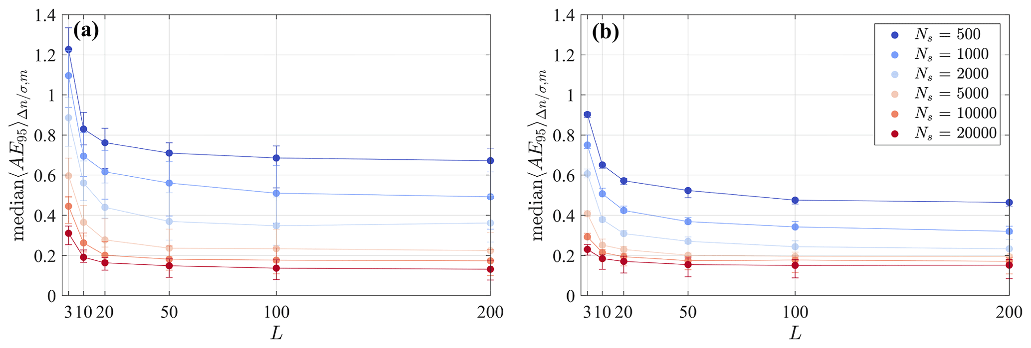
Figure 2Median of the AE95 for all the tested half wavelengths, , and the number of iterations, m. (a) AE95 of the mean field, gm, and (b) AE95 of the variance field, vm. The error bars span the interquartile range.
To verify the analytical response of the mean and variance of the scalar field, f, a numerical estimator of the response is defined as the median in the space of the ratio between the field reconstructed via LiSBOA and the expected value of the synthetic input, as follows:
In the calculation of the numerical response through Eq. (12), the influence of the edges is removed by rejecting points closer than Rmax to the boundaries of the numerical domain. Furthermore, the zero crossings of the synthetic sine function () are excluded to avoid singularities. A comparison between the actual and the theoretical response (Eq. 5) for several wavelengths of the input function is reported in Fig. 3 for the case with the highest number of samples Ns=20 000. An excellent agreement is observed between the theoretical prediction and the Monte Carlo outcome, which indicates that, in the limit of negligible statistical error (large L) and adequate sampling (large Ns and near-uniform distributed samples), the response approaches the predictions obtained from the developed theoretical framework.
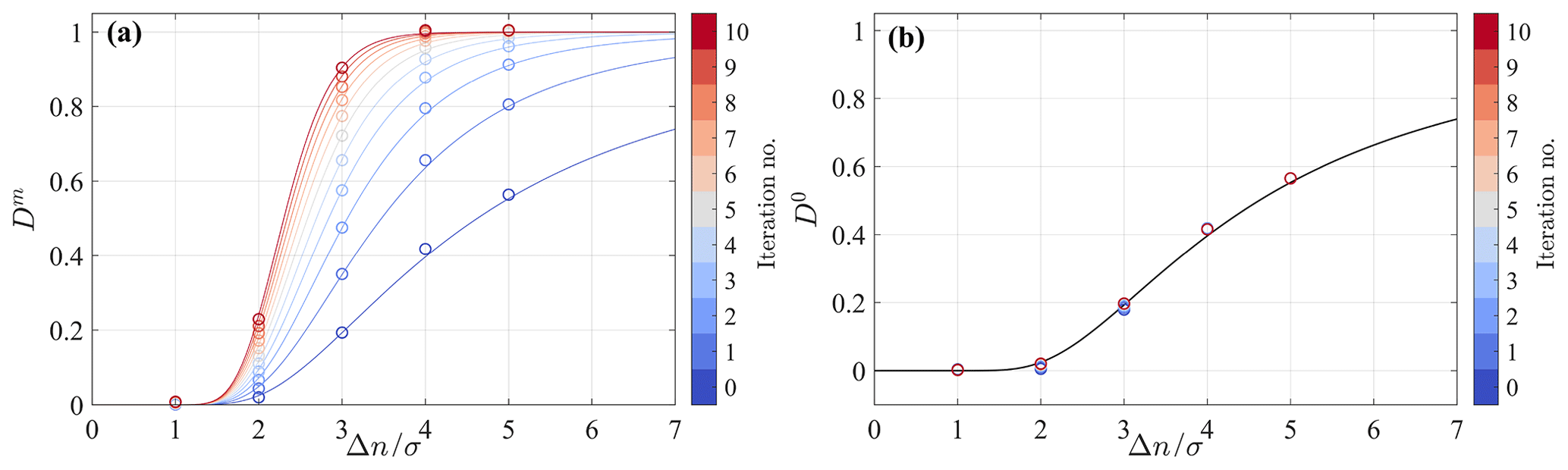
The trend of the response of the mean (Fig. 3a) suggests that, for a given wavelength, the same response can be achieved for an infinite number of combinations σ−m, and specifically, a larger σ requires a larger number of iterations, m, to achieve a certain response, Dm. It is noteworthy that, for a smaller number of iterations, m, the slope of the response function is lower. This feature can be beneficial for practical applications for which the LiSBOA response will have small changes for small variations of Δn. However, a lower slope of the response function can be disadvantageous for short wavelength noise suppression. Figure 3b confirms that the response of the variance and, similarly for higher-order statistics, is not a function of the total number of iterations, m, and is equal to the response of the mean for the 0th iteration, D0.
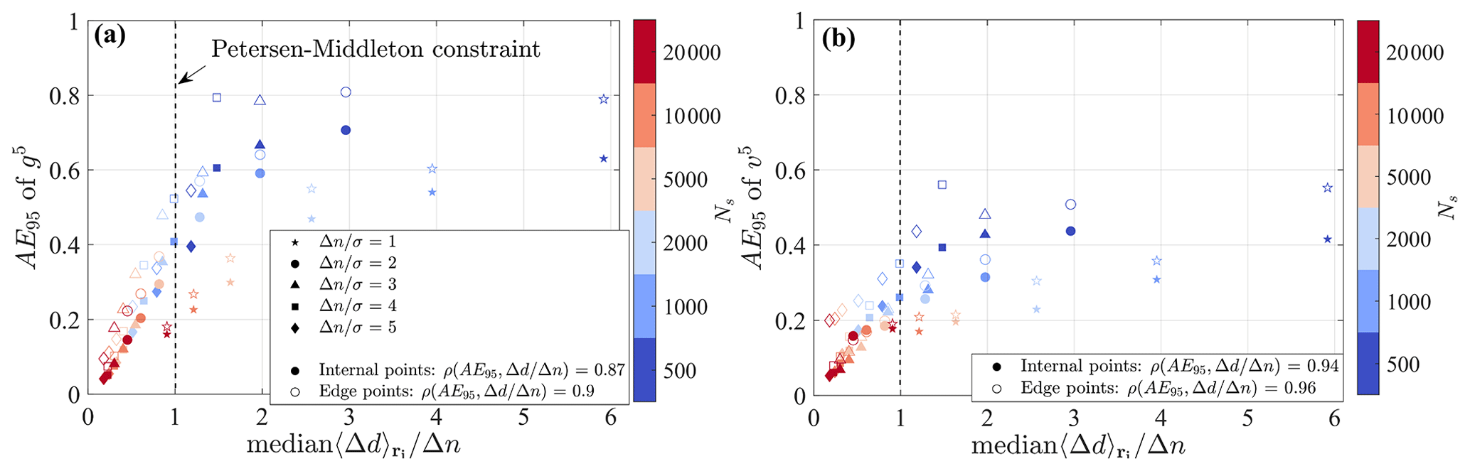
Figure 4AE95 as a function of the random data spacing (Eq. 7) for the case with m=5, N=20 000, and L=200. (a) Error on the mean and (b) error on the variance. The full symbols refer to points not affected by the presence of the finite boundaries of the domain, while the empty symbols are taken within a distance of less than Rmax from the boundaries.
Finally, the link between error and the random data spacing, Δd, is investigated. In Fig. 4, the discrepancy with respect to theory quantified by the AE95 is plotted versus the random data spacing normalized by the half wavelength for a fixed total number of iterations m=5. The values displayed on the x axis represent the median over all grid points, ri. This analysis reveals a strong correlation between the normalized random data spacing and the error. This analysis corroborates that, in the limit of negligible statistical error (i.e., a high number of realizations, L), uncertainty is mainly driven by the local data density normalized by the wavelength, which is related to the Petersen–Middleton criterion. Indeed, the cases satisfying the Petersen–Middleton constraint (Eq. 8) are those exhibiting an AE95 smaller than ∼40 % of the amplitude of the harmonic function for both the mean and variance. However, if a smaller error is needed, it will be necessary to reduce the maximum threshold value for .
An efficient application of LiSBOA to lidar data relies on the appropriate selection of the parameters of the algorithm, namely the fundamental half wavelengths, Δn0, the smoothing parameter, σ, the number of iterations, m, and the spatial discretization of the Cartesian grid, dx. Furthermore, the data collection strategy must be designed to ensure adequate sampling of the spatial wavelengths of interest so that the Petersen–Middleton constraint (Eq. 8) is satisfied. In this section, we show that the underpinning theory of LiSBOA, along with an estimate of the properties of the flow under investigation, can guide the optimal design of a lidar experiment and evaluation of the statistics for a turbulent ergodic flow. The whole procedure can be divided into three phases, namely characterization of the flow, design of the experiment, and reconstruction of the statistics from the collected data set.
First, the integral quantities of the flow under investigation required for the application of LiSBOA need to be estimated, such as extension of the spatial domain of interest, characteristic length scales, integral timescale, τ, characteristic temporal variance of the velocity, , and expected total sampling time, T, which depends on the typical duration of stationary boundary conditions over the domain. These estimates can be based on previous studies available in the literature, numerical simulations, or preliminary measurements.
Then, it is necessary to define the fundamental half wavelengths, Δn0, which are required for the coordinate scaling (Eq. 6). Imposing the fundamental half wavelengths equal to (or even smaller than) the estimated characteristic length scales of the smallest spatial features of interest in the flow is advisable. This ensures isotropy of the mode associated with the fundamental half wavelength (and all the modes characterized by the same degree of anisotropy) and guides the selection of the main input parameters of the LiSBOA algorithm, i.e., smoothing parameter, σ, and number of iterations, m. Indeed, Δn0 can be considered as the cut-off half wavelength of the spatial low-pass filter represented by the LiSBOA operator. To this end, it is necessary to select σ and m to obtain a response of the mean associated with the fundamental mode, , as close as possible to one. After the coordinate scaling (Eq. 6), the response of the fundamental mode is universal, and it is reported in Fig. 5. For instance, if we select a response equal to 0.95, then all the points lying on the isocontour defined by the equality give, in theory, the same response for the mean of the scalar field f. This implies that an infinite number of combinations σ−m allow us to obtain a response of the mean equal to the selected value. However, with increasing σ, the response at the 0th iteration, , reduces, which indicates a lower response for higher-order statistics. For the LiSBOA application, the following aspects should be also considered:
-
the smaller σ, the smaller the radius of influence of LiSBOA, Rmax, and, thus, the lower the number of samples averaged per grid node, Nexp, and the greater the statistical uncertainty;
-
an excessively large m can lead to overfitting of the experimental data and noise amplification (Barnes, 1964);
-
the higher m, the higher the slope of the response function (see Fig. 3), which improves the damping of high-frequency noise, but it produces a larger variation in the response of the mean with different spatial wavelengths; and
-
the radius of influence Rmax (and therefore σ) can affect the data spacing Δd in case of nonuniform data distribution.
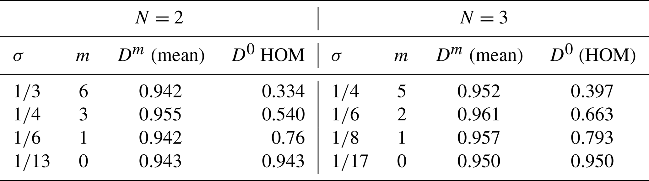
A few handy combinations of smoothing parameters and total iterations for are provided in Table 2. As mentioned above, all these σ−m pairs allow us to achieve roughly the same response for the mean, while the response for the higher-order statistics reduces with an increasing number of iterations, m.
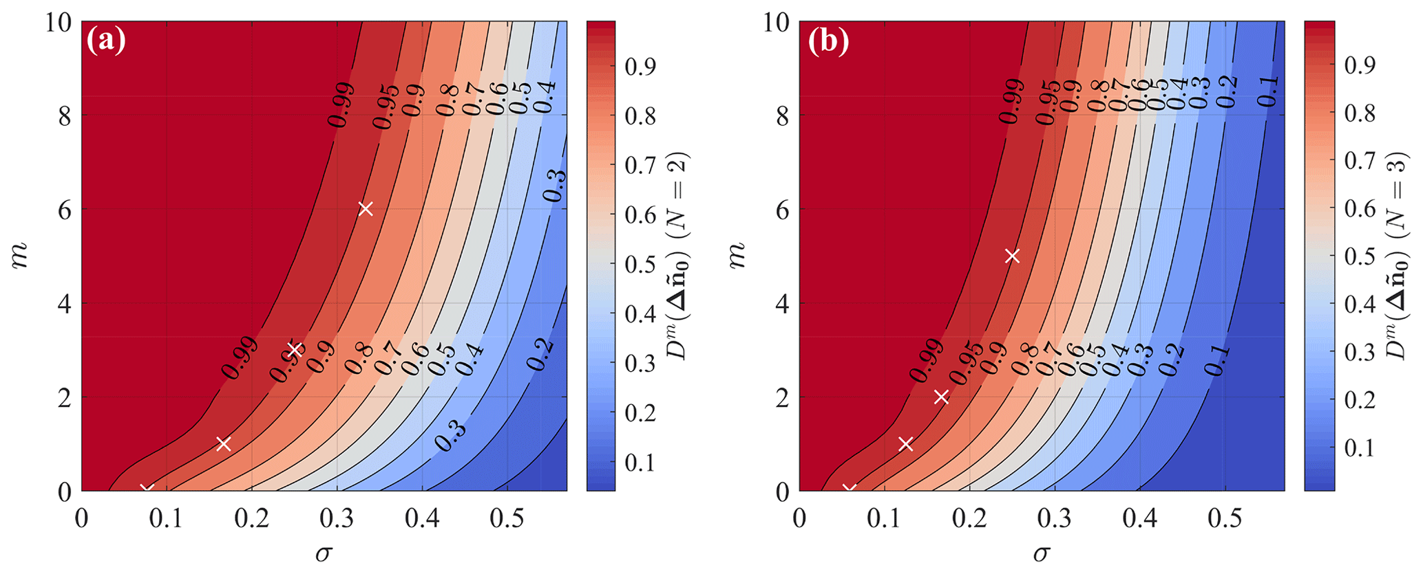
Figure 5Response of the fundamental mode in the scaled coordinates as a function of the number of iterations and the smoothing parameter. (a) 2D LiSBOA and (b) 3D LiSBOA. The white crosses indicate the pairs σ−m provided in Table 2.
Table 2Selected combinations of σ and m for achieving a ∼95 % recovery of the mean of the selected fundamental half wavelength and associated response of the higher-order moments (HOM).
As a final remark about the selection of Δn0, we should consider that, if the fundamental half wavelength is too large compared to the dominant modes in the flow, small-scale spatial oscillations of f will be smoothed out during the calculation of the mean, with the consequence of underestimated gradients and incorrect estimates of the high-order statistics due to the dispersive stresses (Arenas et al., 2019). On the other hand, the selection of an overly small Δn0 would require an excessively fine data spacing to satisfy the Petersen–Middleton constraint (Eq. 8), which may lead to an overly long sampling time, or it may even exceed the sampling capabilities of the lidar.
The optimal lidar scanning strategy aimed to characterize atmospheric turbulent flows implies finding a trade-off between a sufficiently fine data spacing, which is quantified through Δd in the present work (Eq. 7), and an adequate number of time realizations, L, to reduce the temporal statistical uncertainty. Considering a total sampling period, T, for which statistical stationarity can be assumed, and a pulsed lidar that scans Nr points evenly spaced along the lidar laser beam, with a range gate Δr and accumulation time τa, the total number of collected velocity samples is then equal to . The angular resolution of the lidar scanning head in azimuth (Δθ for plan position indicators, PPIs), elevation (Δβ, for RHIs), or both axes (for volumetric scans) can be selected to modify the angular spacing between consecutive lines of sight (i.e., the data spacing) and the total sampling period for a single scan, τs (i.e., the number of realizations, L).
The design of a lidar scan aiming to reconstruct turbulent statistics of an ergodic flow through LiSBOA can be formalized as a two-objective (or Pareto front) optimization problem. The first cost function of the Pareto front, which is referred to as ϵI, is the percentage of grid nodes for which the Petersen–Middleton constraint, applied to the smallest half wavelength of interest (i.e., Δn0), is not satisfied. With respect to the scaled reference frame, this can be expressed as follows:
where the square brackets are Iverson brackets, and Ni is the total number of nodes in the Cartesian grid, ri. For a more conservative formulation, rejecting all the points with a distance smaller than Rmax from an undersampled grid node, i.e., with , is recommended. This condition will ensure that the statistics are based solely on regions that are adequately sampled. The cost function ϵI depends not only on the angular resolution but also on Rmax, which is equal to 3σ in this work. In general, increasing σ results in a larger number of samples considered for the calculation of the statistics at each grid point ri and, thus, in a reduction in ϵI. Therefore, a larger σ entails a larger percentage of the spatial domain fulfilling the Petersen–Middleton constraint. The smoothing parameter, σ, also plays a fundamental role in the response of higher-order statistical moments. Specifically, if the reconstruction of the variance or higher-order statistics is important, the response should be included in the Pareto front analysis as an additional constraint.
The second cost function for the optimal design of lidar scans, ϵII, is equal to the standard deviation of the sample mean, which, for an autocorrelated signal, is (Bayley and Hammersley, 1946) as follows:
where ρp is the autocorrelation function at lag p, τ is the integral timescale, and the approximation is based on George et al. (1978). The velocity variance, , and the autocorrelation, ρp, are functions of space; however, to a good degree of approximation, they can be replaced by a representative value and be considered as being uniform in space. Figure 6 shows the standard deviation of the sample mean normalized by the standard deviation of the velocity as a function of the number of realizations, L, and for different integral timescales, τ. It is noteworthy that the standard deviation of the sample mean represents the uncertainty of the time average of each measurement point, rj, while the final uncertainty of the mean field at the grid nodes ri is generally reduced due to the spatial averaging process intrinsic to LiSBOA. It is noteworthy that the estimates of the statistical error obtained through LiSBOA do not consider other sources of error, such as accuracy of the instruments and spatial averaging due to the lidar measuring process (Rye and Hardesty, 1993; O'Connor et al., 2010; Puccioni and Iungo, 2020). Eventually, other error estimates can be coupled with the sampling error estimated through LiSBOA for a more comprehensive error analysis (Wheeler and Ganji, 2010b). Furthermore, LiSBOA allows the calculation of velocity statistics, including contributions of eddies with different sizes, which span from the largest eddy advected within the total sampling time to the smallest eddy detectable for a given accumulation time (Puccioni and Iungo, 2020). Therefore, a careful preprocessing of the lidar data should eventually be performed to remove contributions due to nonturbulent mesoscale eddies (Högström et al., 2002; Metzger et al., 2007; O'Connor et al., 2010).

Figure 6Standard deviation of the sample mean normalized by the standard deviation of velocity as a function of the number of realizations, L, and for different values of the ratio between the integral timescale and the sampling time, .
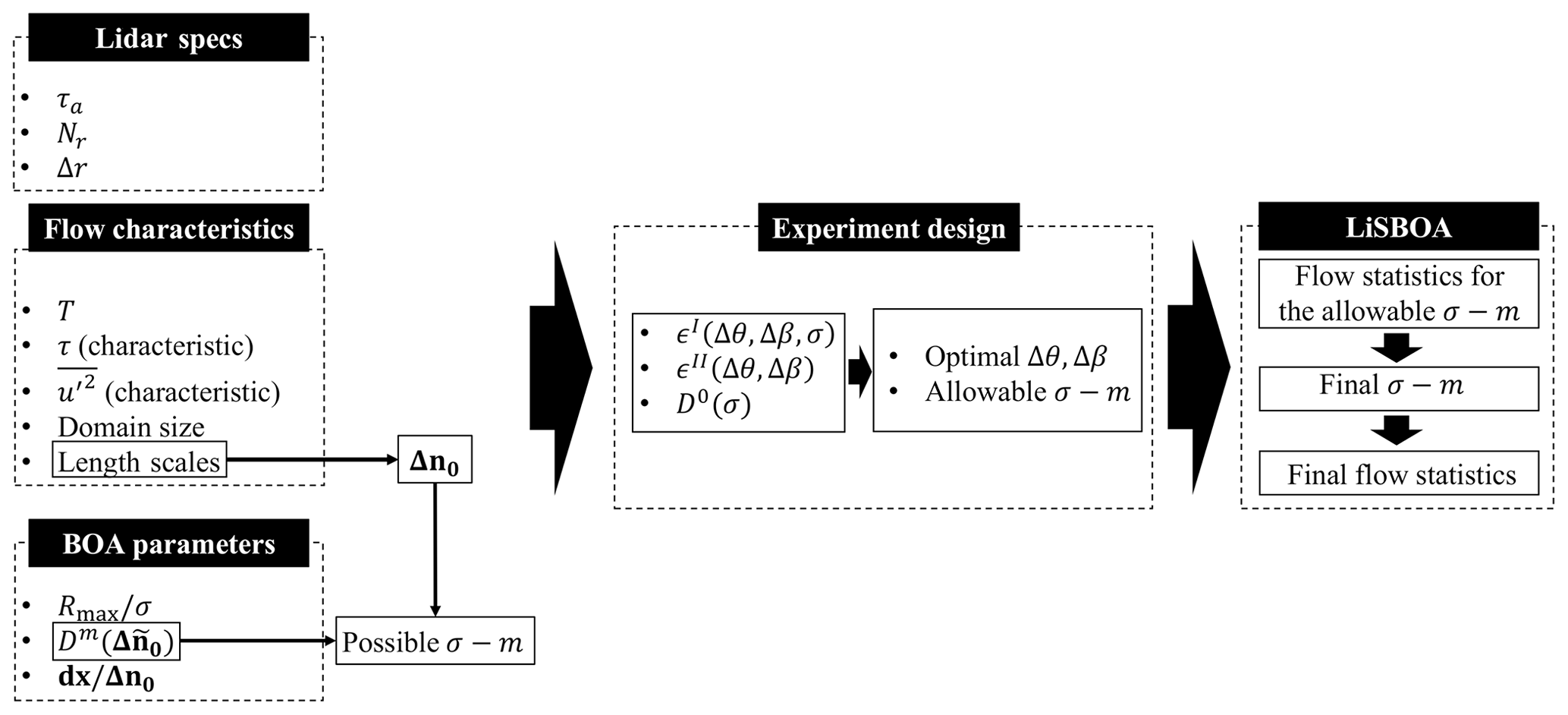
Figure 7Schematic of the LiSBOA procedure for the optimal design of lidar scans and reconstruction of the statistics for a turbulent ergodic flow.
The whole procedure for the design of a lidar scan and retrieval of the statistics is reported in the flow chart of Fig. 7. Summarizing, from a preliminary analysis of the velocity field under investigation, we estimate the maximum total sampling time, T, the characteristic integral timescale, τ, the characteristic velocity variance, , and the fundamental half wavelengths, Δn0. This information, together with the settings of the lidar (namely the accumulation time, τa, the number of points per beam, Nr, and the gate length, Δr), allow the generation of the Pareto front as a function of Δθ and/or Δβ and for different values of σ. Based on the specific goals of the lidar campaign in terms of the coverage of the selected domain (i.e., ϵI), the statistical significance of the data (i.e., ϵII) and, eventually, the response of the higher-order statistical moments (i.e., ), the LiSBOA user should select the optimal angular resolution, Δθ and/or Δβ, and the set of allowable σ values. Due to the abovementioned nonideal effects on LiSBOA, the selection of σ is finalized during the postprocessing phase when the lidar data set is available and the statistics can be calculated for different pairs of σ−m values. For the resolution of the Cartesian grid, Koch et al. (1983) suggested that it should be chosen as a fraction of the data spacing, which, in turn, is linked to the fundamental half wavelength. The same author suggested a grid spacing included in the range . In this work, we have used , which ensures a good grid resolution with acceptable computational costs.
By following the steps outlined in the present section, the mean, variance, or even higher-order statistical moments of the velocity field can be accurately reconstructed for the wavelengths of interest. It is worth mentioning that the LiSBOA of wind lidar data should always be combined with a robust quality control process of the raw measurements. Indeed, the space–time averaging operated by LiSBOA makes the data analysis sensitive to the presence of data outliers, which need to be identified and rejected beforehand to prevent contamination of the final statistics. The interested reader is referred to Manninen et al. (2016), Beck and Kühn (2017), and Vakkari et al. (2019) for more information on quality control of lidar data. On a final note, for applications of LiSBOA, the uncontrollable environmental conditions and the uncertainty in the flow characteristics needed, as the input of LiSBOA may pose some challenges, will be discussed more in detail in Sect. 6.
The LiSBOA algorithm is applied to a synthetic data set generated through the virtual lidar technique to assess accuracy in the calculation of statistics for a wind turbine wake probed through a scanning lidar installed on the turbine nacelle. For this purpose, a simulator of a scanning Doppler pulsed wind lidar is implemented to extract the line-of-sight velocity from a numerical velocity field produced through high-fidelity large eddy simulations (LES). Due to their simplicity and low computational costs, lidar simulators have been widely used for the assessment of postprocessing algorithms of lidar data and scan design procedures (Mann et al., 2010; Stawiarski et al., 2015; Lundquist et al., 2015; Mirocha et al., 2015).
As a case study, we use the LES data set of the flow past of a single turbine with the same characteristics of the 5-MW NREL (National Renewable Energy Laboratory) reference wind turbine (Jonkman et al., 2009). The rotor is three bladed and has a diameter D=126 m. The tip-to-speed ratio of the turbine is set to its optimal value of 7.5. A uniform incoming wind with a free stream velocity of U∞=10 m s−1 and turbulence intensity of 3.6 % is considered. The rotor is simulated through an actuator disk with rotation, while the drag of the nacelle is taken into account using an immersed boundary method (Ciri et al., 2017). More details on the LES solver can be found in Santoni et al. (2015). The computational domain has dimensions () in the streamwise, spanwise, and vertical directions, respectively, and it is discretized with uniformly spaced grid points, respectively, resulting in a spacing of dx=0.0125D, dy=0.025D and dz=0.0202D. A radiative condition is imposed at the outlet (Orlanski, 1976), while periodicity is applied in the spanwise direction. For the sake of generality, a uniform incoming wind is generated by imposing free-slip conditions at the top and bottom of the numerical domain. Ergodic velocity vector fields are available for a total time of T=750 s.
For the estimation of the flow characteristics necessary for the scan design, the azimuthally averaged mean and standard deviation of streamwise velocity, as well as the integral timescale are considered (Fig. 8). The use of cylindrical coordinates is justified by the axisymmetry of the statistics of the wake velocity field generated by a turbine operating in a uniform velocity field (Iungo et al., 2013a; Viola et al., 2014; Ashton et al., 2016).
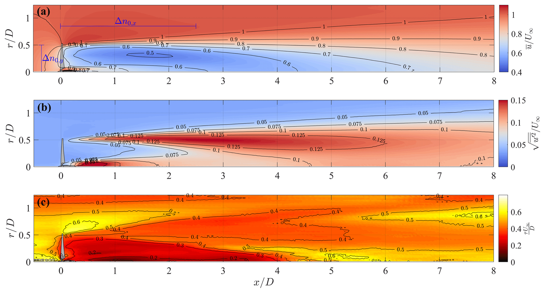
Figure 8Azimuthally averaged statistics of the LES streamwise velocity field. (a) Mean value, (b) standard deviation, and (c) integral timescale.
The streamwise LES velocity field shows the presence of a higher-velocity jet surrounding the nacelle, while exhibits a clear minimum placed at (Fig. 8a). These flow features are consistent with the double Gaussian velocity profile typically observed in the near-wake region (Aitken and Lundquist, 2014). In Fig. 8b, the standard deviation of the streamwise velocity has high values in the very near wake () in the proximity of the rotor axis, which is most probably connected with the vorticity structures generated in proximity of the rotor hub and their dynamics (Iungo et al., 2013a; Viola et al., 2014; Ashton et al., 2016). Similarly, enhanced values of the velocity standard deviation occur at the wake boundary (), which are connected with the formation and dynamics of the helicoidal tip vortices (Ivanell et al., 2010; Debnath et al., 2017c). A peak of is observed around (), which can be considered as being the formation length of the tip vortices. The integral timescale is evaluated by integrating the sample biased autocorrelation function of the time series of u up to the first zero crossing (Zieba and Ramza, 2011). The integral timescale is generally smaller within the wake than for the typical values observed in the free stream, which is consistent with the smaller dimensions of the wake vorticity structures compared to the larger energy-containing structures present in the incoming turbulent wind.
To reconstruct the mentioned flow features, the fundamental half wavelengths in the spanwise and vertical directions selected for this application of LiSBOA are , which allows the retrieval of spatial features of the velocity field as small as the rotor blade in the cross-stream direction, which are typically observed in the near wake (Aitken and Lundquist, 2014; Santoni et al., 2017). Furthermore, considering the streamwise elongation of the isocontours of the flow statistics shown in Fig. 8a, a conservative value of the fundamental half wavelength in the x direction is selected. This information could also have been inferred from previous studies (e.g., Chamorro and Porté-Agel, 2010; Abkar and Porté-Agel, 2013; Zhan et al., 2019).

Figure 9Azimuthally averaged energy spectra of the LES velocity fields. (a) Mean streamwise velocity on the physical domain, (b) variance of streamwise velocity on the physical domain, (c) mean streamwise velocity on the scaled domain, and (d) variance of streamwise velocity on the scaled domain. The blue dashed line indicates wavenumbers reconstructed with response equal to .
The availability of the LES data set allows the testing of the relevance of the selected Δn0 by evaluating the 3D energy spectrum of and in the physical and scaled reference frames (Eq. 6). The spectra are azimuthally averaged by exploiting the axisymmetry of the wake. The spectra in the physical reference frame (Fig. 9a and b) reveal the clear signature of a streamwise elongation of the energy-containing scales for both velocity mean and variance, with the energy being spread over a larger range of frequencies in the radial direction compared to the streamwise direction. After the scaling (Fig. 9c and d), the spectra become more isotropic in the spectral domain, namely the energy is distributed equally along the and axes. In Fig. 9c, the blue dashed line represents the intersection with the – plane of the spherical isosurface that, in the wavenumber space, is characterized by . All the modes contained within that sphere are reconstructed with a response Dm>0.95, while higher-frequency features lying outside will be damped. Numerical integration of the 3D energy spectrum shows that 94 % of the total spatial variance of the mean is contained within that sphere, which ensures that the energy-containing modes in the mean flow are adequately reconstructed with the selected parameters.
The analysis of the flow statistics reported in Fig. 8 enables estimates of flow parameters needed as input for LiSBOA. For instance, the wake region is characterized by and 0.4 (τ≈5 s).
A main limitation of lidars is represented by the spatiotemporal averaging of the velocity field, which is connected with the acquisition process. Three different types of smoothing mechanisms can occur during the lidar sampling. The first is the averaging along the laser beam direction within each range gate, which has commonly been modeled through the convolution of the actual velocity field with a weighting function within the measurement volume (Smalikho, 1995; Frehlich, 1997; Sathe et al., 2011). The second process is the time averaging associated with the sampling period required to achieve a backscattered signal with adequate intensity (O'Connor et al., 2010; Sathe et al., 2011), while the last one is the transverse averaging (azimuth-wise or elevation-wise averaging) occurring in case of a scanning lidar operating in continuous mode (Stawiarski et al., 2013). These filtering processes lead to a significant underestimation of the turbulence intensity (Sathe et al., 2011), an overestimation of integral length scales (Stawiarski et al., 2015), and a damping of energy spectra for increasing wavenumbers (Risan et al., 2018; Puccioni and Iungo, 2020).
A total of three versions of a lidar simulator are implemented for this work. The simplest one is referred to as ideal lidar, which samples the LES velocity field at the experimental points through a nearest-neighbor interpolation. This method minimizes the turbulence damping while retaining the geometry of the scan and the projection of the wind velocity vector onto the laser beam direction. The second version of the lidar simulator reproduces a step-stare lidar, i.e., the lidar scans for the entire duration of the accumulation time at a fixed direction of the lidar laser beam. A total of two filtering processes take place for this configuration, namely beam-wise convolution and time averaging. To model the beam-wise average, the retrieval process of the Doppler lidar is reproduced using a spatial convolution (Mann et al., 2010) as follows:
where n is the lidar laser beam direction, u is the instantaneous velocity vector, and the dot indicates scalar product. A triangular weighting function ϕ(s) was proposed by Mann et al. (2010) as follows:
where Δr is the gate length. The former expression is valid, assuming matching time windowing, i.e., gate length equal to the pulse width, and the velocity value is retrieved based on the first momentum of the backscattering spectrum. Despite its simplicity, Eq. (16) has shown to estimate realistic turbulence attenuation due to the beam-wise averaging process of a pulsed Doppler wind lidar (Mann et al., 2009). Furthermore, time averaging occurs due to the accumulation time necessary for the lidar to acquire a velocity signal with sufficient intensity and, thus, signal-to-noise-ratio. This process is modeled through a window average within the acquisition interval of each beam. For the sampling of the LES velocity field in space and time, a nearest-neighbor interpolation method is used.
The third version of the lidar simulator mimics a pulsed lidar operating in continuous mode and performing PPI scans, where, in addition to the beam-wise convolution and time averaging, azimuth-wise averaging occurs due to the variation in the lidar azimuth angle of the scanning head during the scan. The latter is taken into account by adding an azimuthal averaging to the time average, among all data points included within the following angular sector:
where r is the radial distance from the emitter, while θ and β are the associated azimuth and elevation angles, respectively. The subscript p refers to the pth lidar data point. Following the suggestions by Stawiarski et al. (2013), the out-of-plane thickness, Δz, is considered equal to the length of the diagonal of a cell of the computational grid.
It is noteworthy that the accuracy estimated through the present analysis only includes error due to the sampling in time and space and data retrieval. Other error sources, such as the accuracy of the instrument (Rye and Hardesty, 1993; O'Connor et al., 2010), are not included and should be coupled to the LiSBOA estimates for a more general error quantification (Wheeler and Ganji, 2010b).
Figure 10a shows a snapshot of the streamwise velocity field over the horizontal plane at hub height obtained from the LES. The respective data of the radial velocity obtained from the three versions of the lidar simulator, by considering a scanning pulsed wind lidar deployed at the turbine location and at hub height, highlight the increased spatial smoothing of the radial velocity field by adding the various averaging processes connected with the lidar measuring process, namely beam-wise, temporal, and azimuthal averaging (Fig. 10).
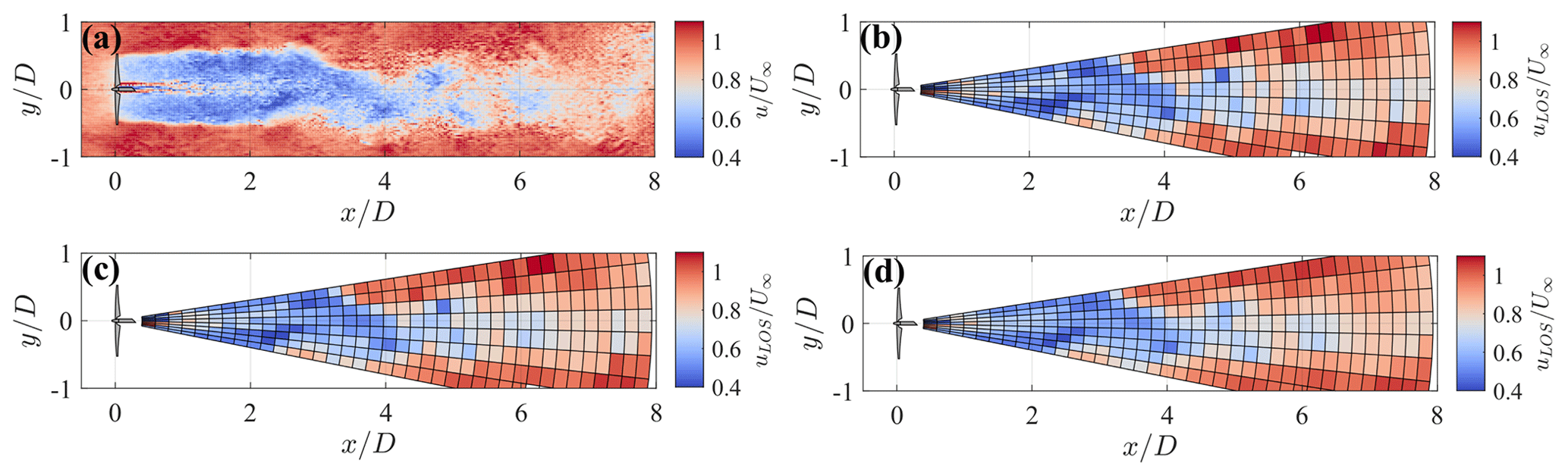
Figure 10Snapshot at the hub height horizontal plane of the wake generated by the 5-MW NREL reference wind turbine. (a) LES streamwise velocity. (b) Ideal virtual lidar with angular resolution , zero elevation, accumulation time τa=0.5 s, and gate length Δr=25 m. (c) Step-stare virtual lidar (same settings). (d) Continuous mode virtual lidar (same settings).
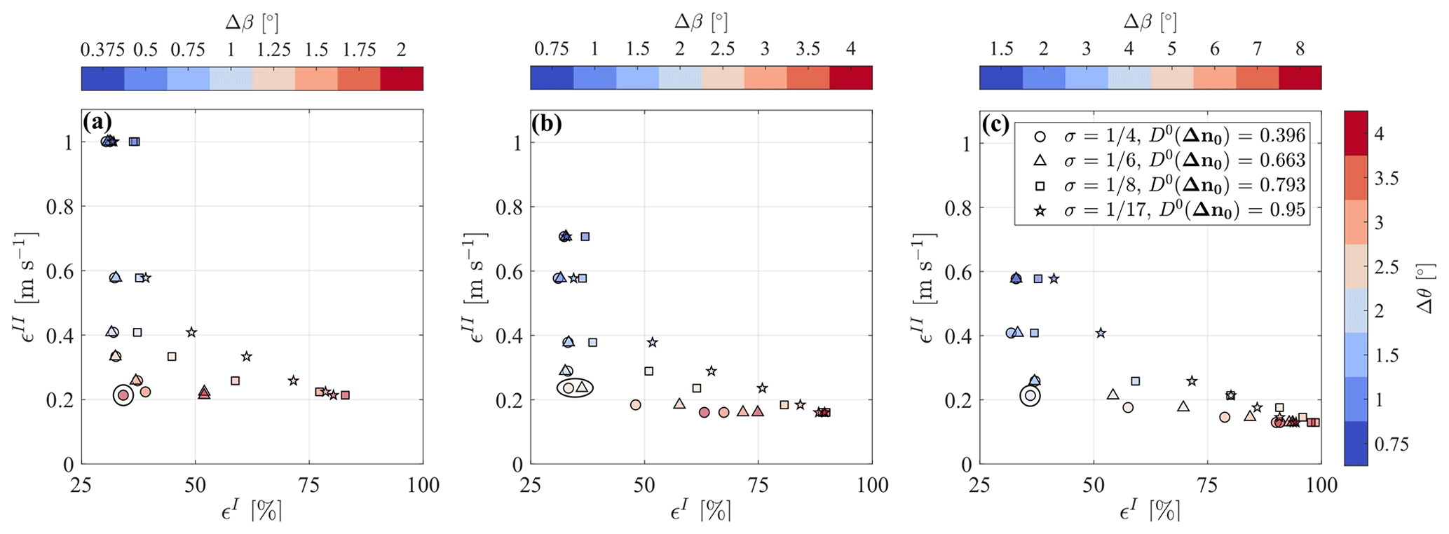
Figure 11Pareto front for the design of the optimal lidar scan for the LES data set for different combinations. (a) . (b) . (c) . The circle indicates the selected optimal configurations.
The application of LiSBOA requires the provision of technical specifications of the lidar, specifically accumulation time, τa, number of gates, Nr, and gate length, Δr. For this work, these parameters are selected based on the typical settings of the WindCube 200S and StreamLine XR lidars (El-Asha et al., 2017; Zhan et al., 2019, 2020), namely τa=0.5 s, Nr=39, and Δr=25 m. Furthermore, to probe the wake region, a volumetric scan, including several PPI scans, with azimuth and elevation angles uniformly spanning the range , with a constant angular resolution in both azimuth and elevation being selected, is conducted, while the virtual lidar is placed at the turbine hub.
With the information provided about the flow under investigation and the lidar system, it is possible to draw the Pareto front for the optimization of the lidar scan as a function of different combinations of angular resolutions of the lidar scanning head, Δθ and Δβ, and the smoothing parameter of LiSBOA, σ, as shown in Fig. 11 for the case under investigation.
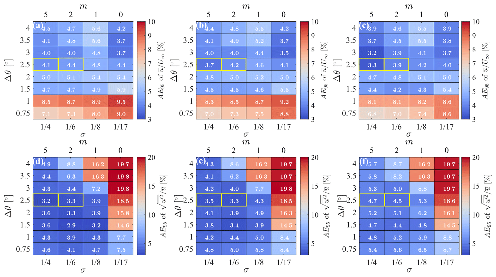
Figure 12Error analysis of LiSBOA applied to virtual radial velocity fields: (a, d) ideal lidar; (b, e) step-stare lidar; (c, f) continuous lidar; (a, b, c) mean streamwise velocity; (d, e, f) streamwise turbulence intensity. The optimal configurations are highlighted in yellow.
For the optimization of the lidar scan, the lidar angular resolution, Δθ, is evenly varied for a total number of seven cases, from 0.75 to 4∘, whereas three values of the ratio , namely 0.5, 1, and 2, are tested separately. The four values of σ recommended in Table 2, to achieve a response of the mean , are considered here. In Fig. 11, markers indicate the different σ and, thus, the response of high-order statistical moments, . Changing the ratio affects the optimal Δθ (circled in black in Fig. 11); however, it has a negligible effect on the magnitude of the optimal ϵI and ϵII. For the rest of the discussion, we select the setup , as suggested by Fuertes Carbajo and Porté-Agel (2018). The Pareto front for (Fig. 11b) shows that increasing Δθ from 0.75 up to 2.5∘ drastically reduces the uncertainty on the mean (ϵII) by roughly 70 % but does not significantly affect data loss consequent to the enforcement of the Petersen–Middleton constraint (ϵI). For larger angular resolutions, the statistical significance improves just marginally but at the cost of a relevant data loss. For , in particular, ϵI becomes extremely sensitive to σ, with the most severe data loss occurring for small σ (i.e., small Rmax). The Pareto front also shows that, to achieve a higher response for the higher-order statistics, generally entails an increased data loss and/or statistical uncertainty of the mean. This analysis suggests that the optimal lidar scan for the reconstruction of the mean velocity field should be performed with and or .
Virtual lidar simulations are performed for all the values of angular resolution utilized in the Pareto front reported in Fig. 11. The streamwise component is estimated from the line-of-sight velocity through an equivalent velocity approach (Zhan et al., 2019). The latter states that, for small elevation angles (i.e., β≪1) and under the assumption of negligible vertical velocity compared to the horizontal component (i.e., ) and uniform wind direction, θw, a proxy for the streamwise velocity can be calculated as follows:
The mean velocity and turbulence intensity are reconstructed through LiSBOA. The maximum error is quantified through the 95th percentile of the absolute error, AE95, using as reference the LES statistics interpolated on the LiSBOA grid.
Figure 12 reports the AE95 for the flow statistics for all the virtual experiments. The error for the mean field (Fig. 12a–c) is mostly governed by the angular resolution, with a higher error occurring for slower scans. This is a clear consequence of the increased statistical uncertainty due to the limited number of scan repetitions, L, that are achievable for small Δθ values and a fixed total sampling period, T, while AE95 stabilizes for . The trend of the AE95 for , with the pair-smoothing-parameter number of iterations, σ−m, is less significant since the theoretical response of the fundamental mode is ideally equal for all four cases. Conversely, the error on the turbulence intensity (Fig. 12d–f) shows low sensitivity to the angular resolution but a steep increase for small σ values, which is due to the reduction in the radius of influence, Rmax, and the number of points averaged per grid node.
From a more technical standpoint, the error on the mean velocity field, , appears to be relatively insensitive to the type of lidar scan, with the spatial and temporal filtering operated by the step-stare and continuous lidar even being beneficial in some cases. In contrast, the error on the turbulence intensity exhibits a more consistent and opposite trend, with the continuous lidar showing the most severe turbulence damping. This feature has been extensively documented in previous studies, see e.g., Sathe et al. (2011).
This error analysis confirms that the optimal configurations selected through the Pareto front (i.e., , , and ) are arguably optimal in terms of accuracy (AE95 of %–4.1 % and 3.9 %–4.4 % and AE95 of %–4.7 % and 3.3 %–4.5 %, respectively) and data loss (ϵI=33 % and 37 %, respectively).
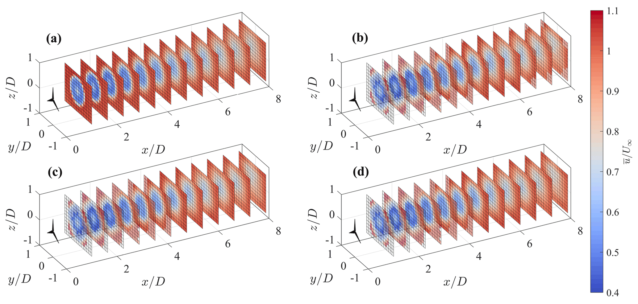
Figure 13Mean streamwise velocity for , , m=5. (a) LES, (b) ideal lidar, (c) step-stare lidar, and (d) continuous mode lidar. The shaded area corresponds to the points rejected after the application of the Petersen–Middleton constraint.

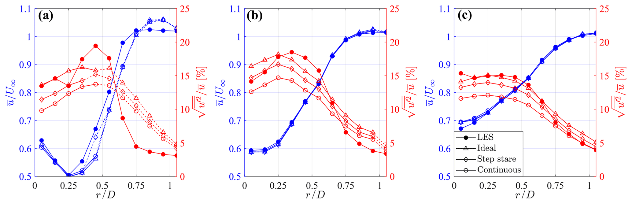
Figure 15Azimuthally averaged profiles of mean streamwise velocity and turbulence intensity for three downstream locations. (a) , (b) , and (c) . The dashed lines correspond to regions rejected after the application of the Petersen–Middleton constraint.
The 3D fields of mean velocity and turbulence intensity calculated over T=750 s through the first optimal configuration, (i.e., , , and m=5), are rendered in Figs. 13 and 14, respectively. Furthermore, in Fig. 15, azimuthally averaged profiles at three downstream locations are also provided for a more insightful comparison. The mean velocity field is reconstructed fairly well, regardless of the type of lidar scan, due to the careful choice of the fundamental half wavelength, Δn0, for this specific flow. On the other hand, the reconstructed turbulence intensity is highly affected by the lidar processing, which leads to visible damping of the velocity variance for the step stare and even more for the continuous mode. The ideal lidar scan, whose acquisition is inherently devoid of any space–time averaging, allows the retrieval of the correct level of turbulence intensity for locations for x≥4D, while in the near wake it struggles to recover the thin turbulent ring observed in the wake shear layer. Indeed, such a short wavelength feature has a small response for the chosen settings of LiSBOA, particularly Δn0 and σ (see Fig. 3b). On the other hand, any attempt to increase the response of the higher-order moments, for instance by reducing the fundamental half wavelengths or decreasing the smoothing and the number of iterations, would result in higher data loss and fewer experimental points per grid node.
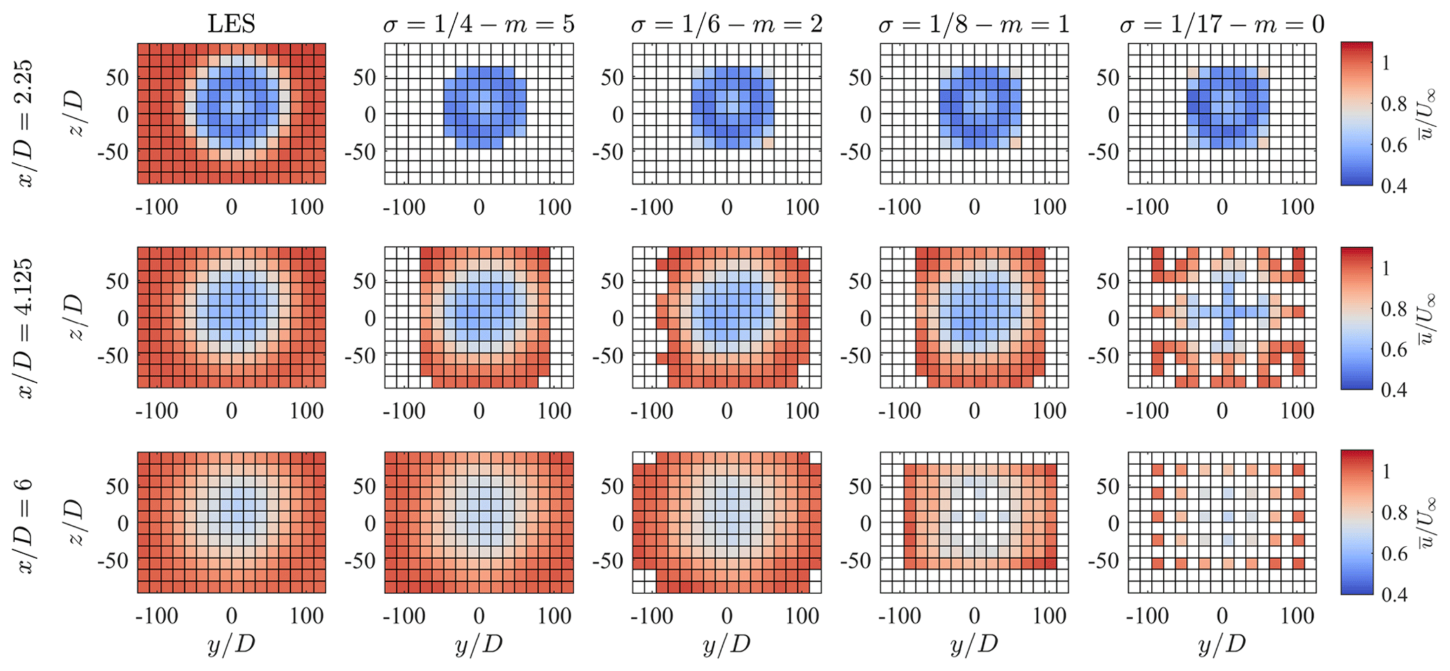
Figure 16Mean streamwise velocity fields obtained through the ideal lidar simulator with over cross-flow planes at three downstream locations and four combinations of σ−m, compared with the corresponding LES data.
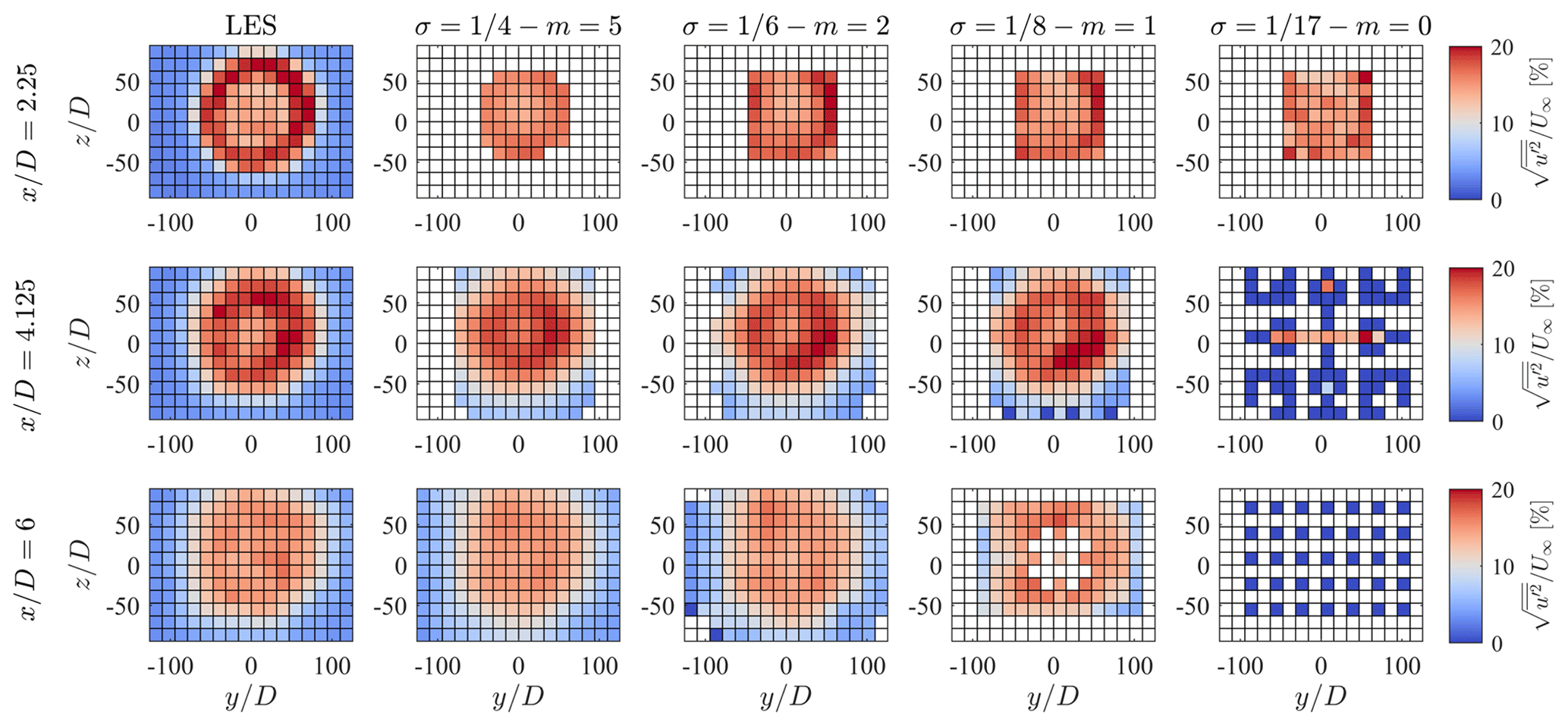
Finally, Figs. 16 and 17 show and over several cross-flow planes and for all the combinations of σ−m tested for the ideal lidar and the optimal angular resolution. For the mean velocity, the most noticeable effect is the increasingly severe data loss as a consequence of the reduction in σ, which indicates as being the most effective setting. The turbulence intensity exhibits, in addition to the data loss, a moderate increase in the maximum value for smaller σ, which is due to the higher response of the higher-order statistics (see Table 2). However, this effect is negligible in the far wake, where the radial diffusion of the initially sharp turbulent shear layer results in a shift of the energy content towards scales with larger Δn, which are fairly well recovered – even for .
LiSBOA can be applied to lidar data sets that are statistically homogeneous as a function time, t. This statistical property can be ensured with two approaches. The first approach consists of considering lidar data collected continuously in time, with a given sampling frequency, for a period where environmental parameters, such as wind speed and direction, Obukhov length, and bulk Richardson number for the atmospheric stability regime, are constrained within prefixed intervals (e.g., Banta et al., 2006; Iungo et al., 2013b; Kumer et al., 2015; Puccioni and Iungo, 2020). For instance, the statistical stationarity of a generic flow signal, α, can be verified through the nonstationary index (IST; Liu et al., 2017) as follows:
where represents time averaging and is the mean value of the variance calculated over consecutive nonoverlapping subperiods. The IST values should be lower than a selected threshold, depending on the specific flow parameter considered (Foken et al., 2004). A second approach to ensure statistical homogeneity of the lidar data set consists of performing a cluster analysis based on environmental parameters, such as those mentioned above. This can be a fruitful alternative when the application of the first approach leads to too short periods with statistical stationarity and, thus, with low accuracy in the calculation of the turbulent statistics. With the clustering approach, larger data sets can be achieved for each cluster, enabling an enhanced statistical convergence (see, e.g., applications of clustering analysis to lidar measurements of wind turbine wakes; Machefaux et al., 2016; Bromm et al., 2018; Iungo et al., 2018; Zhan et al., 2019, 2020).
The results of LiSBOA for the optimal design of wind lidar scans are affected by the selection of the input parameters, such as the total sampling time, T, the integral timescale, τ, the velocity variance, , and the fundamental half wavelength, Δn0. In this section, we will discuss the sensitivity of LiSBOA to these input parameters by considering, as a reference case, the volumetric scan performed with the virtual lidar technique on the LES data set analyzed in Sect. 5. The respective results are summarized in Fig. 18.
The total sampling time, T, directly affects the objective function ϵII through parameter L, which represents the number of realizations. In Fig. 18a–d, different Pareto fronts are generated for the case under investigation, by varying T from 3 min to 1 h. The various Pareto fronts exhibit similar trends for the various values of T and generally higher values of ϵII, so lower statistical accuracy, for smaller T. For all the cases, the optimal configuration is still that selected in Sect. 5, namely –.
For this sensitivity study, the characteristic integral timescale, τ, has been varied between 0 s (completely random uncorrelated data) up to 35 s, with the upper value being based on the largest integral length scale in the atmospheric boundary layer (ABL), according to (ESDU, 1975), and considering an advection velocity of 8 m s−1. The respective Pareto fronts reported in Fig. 18e–h show that the optimal lidar scan is weakly affected by variations of τ, which is an advantageous feature of LiSBOA for applications in which this parameter cannot be estimated from previous investigations or the literature.
Regarding the characteristic velocity variance, , it is a multiplicative parameter for the objective function ϵII (Eq. 14). Therefore, even though it affects the accuracy of the statistics retrieved, it does not alter the selection of the optimal scanning parameters.
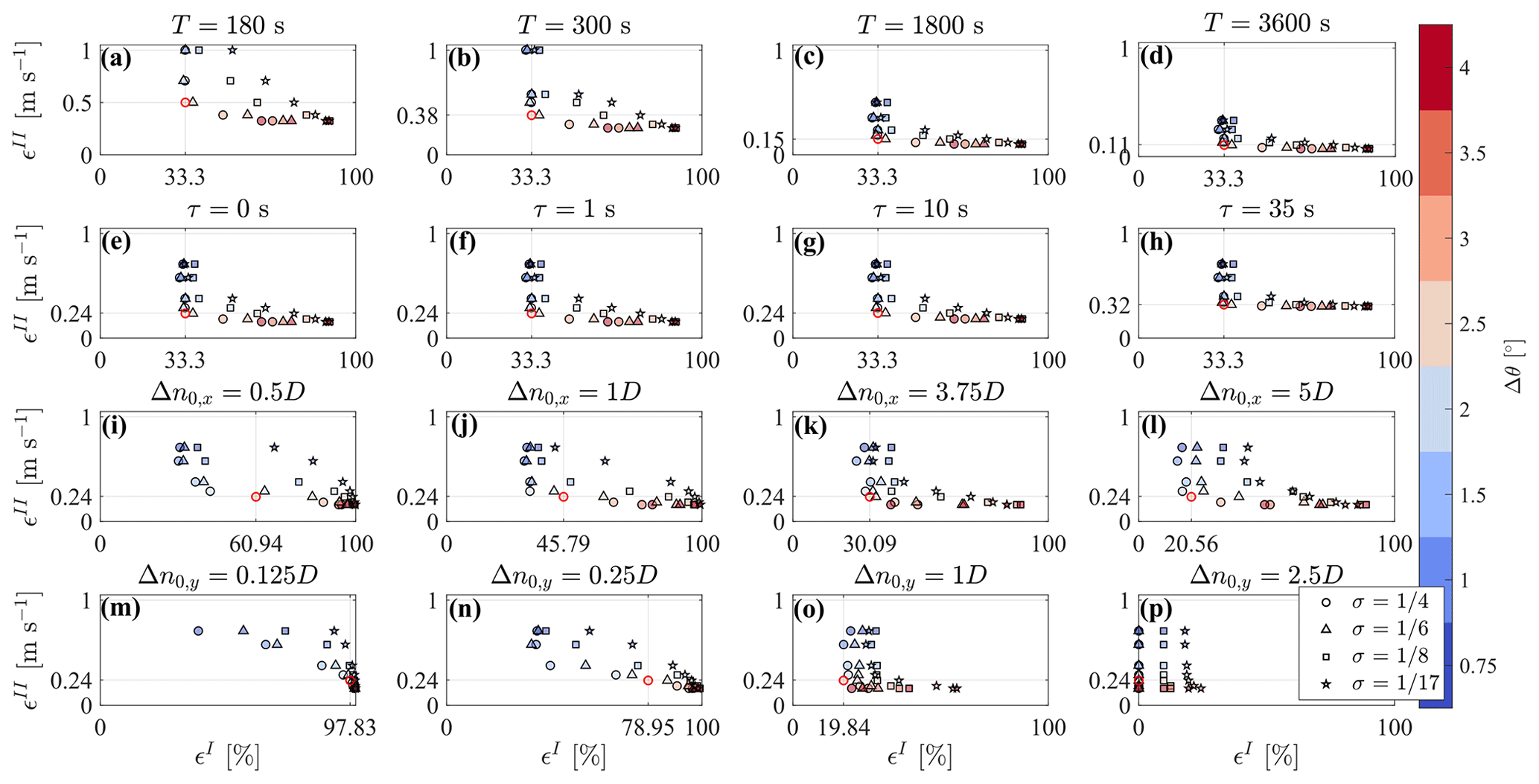
Figure 18Pareto fronts for the design of the volumetric scan for different inputs. (a–d) Sensitivity to total sampling time T. (e–h) Sensitivity to integral timescale, τ. (i–l) Sensitivity to streawmise fundamental half wavelength, Δn0,x. (m–p) Sensitivity to spanwise fundamental half wavelength, Δn0,y. The parameters not indicated at the top of the figures are kept equal to the optimal design case identified in Sect. 5.
The choice of the fundamental half wavelength, Δn0, deserves special attention since it affects both the optimal scan design and retrieval of data statistics. The fundamental half wavelength can be considered as being the cut-off wavelength of the spatial low-pass filtering operated by LiSBOA (Sect. 4). The selection of Δn0 depends mostly on the length of the smallest spatial feature of interest in the flow under investigation, so the Pareto front is likely to be rather sensitive to changes in Δn0. As mentioned in Sect. 4, if the fundamental half wavelengths are too large compared to the predominant spatial modes, the turbulence statistics may be contaminated by over-smoothing and dispersive stresses, whereas overly small Δn0 may require angular and radial resolutions that are too small, a longer sampling period, and, thus, a smaller number of repetitions for a given T. Figure 18i–l shows the Pareto fronts calculated at different Δn0,x. The previously selected optimal setup () still belongs to the optimality frontier. Finally, Fig. 18p–m displays the effect of varying Δn0,y on the Pareto front. Unlike the other cases, the shape of the front is very sensitive to Δn0,y, with a significant increase in data loss, ϵI, consequent to refinements of the angular resolution, Δθ. The Pareto front correctly indicates that finer angular resolutions are needed to adequately sample a velocity field characterized by smaller wavelengths.
For the sake of completeness, the influence of the different fundamental half wavelengths on the statistics is assessed by calculating the AE95 between LiSBOA and LES for the statistics reconstructed using several combinations of Δn0,x and Δn0,y (Fig. 19). Larger values of Δn0,x and Δn0,y produce detrimental effects on the accuracy for both mean velocity and turbulence intensity due to the over-smoothing of the mean velocity and turbulence intensity field and dispersive stresses for the turbulence intensity only. On the other hand, excessively small values of Δn0,y exhibit a slight increase in error as a consequence of the smaller number of samples per grid node. Nonetheless, the most relevant effect, in this case, is represented by the high data loss, as already identified in the Pareto front (e.g., Fig. 18m, n). It is worth noting how the choice of in Sect. 5, which was purely based on physical considerations about the expected relevant modes in the near wake, turned out to be the optimal configuration in terms of the overall error of and .
We acknowledge that the technical specifications required by LiSBOA (namely τa, Nr, and Δr) are dependent on the specific lidar system used, the contingent atmospheric conditions, and the best practices followed by the user. Since these parameters are greatly case dependent, they will not be discussed further in this context. In general, the selection of the accumulation time and gate length is a trade-off between the need to achieve a target maximum range, while keeping a sufficiently fine radial resolution and a sufficient intensity of the backscattered lidar signal. In the case of uncertain environmental conditions, checking, before the deployment, the influence of selected combinations of τa, Nr, and Δr on the Pareto front is recommended.

Figure 19AE95 of the statistics reconstructed from virtual lidar data for different streamwise and spanwise fundamental half wavelengths, for the setup . (a) Mean streamwise velocity. (b) Streamwise turbulence intensity.
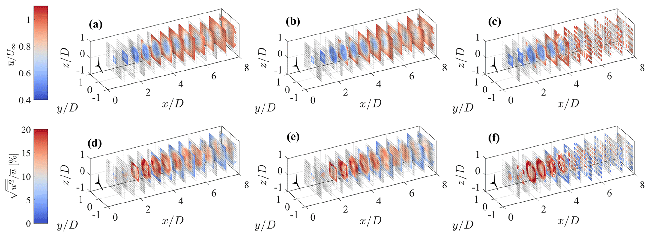
Figure 20Statistics retrieved from a step-stare virtual lidar scan of the LES data set by means of different techniques. (a, d) Delaunay triangulation. (b, e) Linear interpolation. (c, f) Window averaging. (a, b, c) Mean streamwise velocity. (d, e, f) Streamwise turbulence intensity.
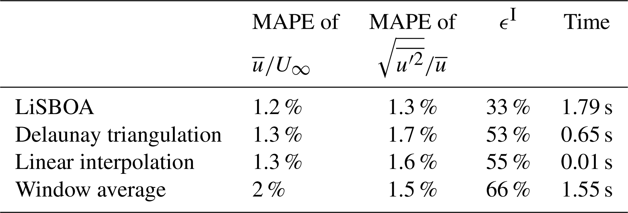
For the sake of completeness, LiSBOA is compared with other widely used techniques for statistical postprocessing of wind lidar data, specifically the Delaunay triangulation (see, e.g., Clive et al., 2011; Trujillo et al., 2011, 2016; Iungo and Porté-Agel, 2014; Machefaux et al., 2015), linear interpolation in spherical coordinates (see, e.g., Mohr and Vaughan, 1979; Fuertes Carbajo and Porté-Agel, 2018), and window averaging (see, e.g., Newsom et al., 2008). Figure 20 shows the mean velocity and turbulence intensity fields retrieved from the considered LES data set through the various techniques for a step-stare virtual lidar scan. The various methods use the same grid as for LiSBOA (see Sect. 5). The voids in the 3D rendering correspond to regions outside of the data distribution for the Delaunay triangulation and linear interpolation (i.e., extrapolation cannot be performed) or bins having a standard error on the mean higher than 15 % of the incoming wind speed for the window average (for an analogy with LiSBOA, see Fig. 4). A qualitative comparison of the results reported in Fig. 20 with those for LiSBOA in Figs. 13c and 14c reveals that LiSBOA is the method enabling the largest spatial coverage for the retrieved statistics for the same lidar scan. From the parameter ϵI, which is reported in Table 3 for the various methods, it is noted that LiSBOA is the method with the lowest data rejection rate (ϵI=33 %), while the largest is for the window average (ϵI=66 %).
Overall, all the methods, except for the window average, have similar accuracy in the retrieval of the mean velocity (see the mean absolute percentage error, MAPE, in Table 3), yet LiSBOA is the method with the lowest error. Furthermore, LiSBOA is the only method not showing artifacts for the retrieval of turbulence intensity over space, such as enhanced turbulence intensity and unexpected peaks, as the significantly lower error on turbulence intensity confirms. This result is in agreement with Trapp and Doswell (2000), where the effectiveness of the Barnes scheme in the suppression of short-wavelength noise compared to linear interpolation was already noted. Finally, the computational time, using MATLAB on a quad-core i7 laptop, is negligible and comparable for all the algorithms considered (∼1–2 s), with only the linear interpolation being considerably faster (Table 3).
Table 3Comparison between LiSBOA and other techniques for the retrieval of mean velocity and turbulence intensity from the LES data set through a virtual lidar scan.
On a final note, it is noteworthy that LiSBOA is currently formulated for a single scalar field, namely a velocity component (radial or equivalent horizontal). However, in principle, this procedure can be extended to vector fields, such as fully 3D velocity fields. Furthermore, other constraints can be added for the optimal scanning design, such as imposing a divergence-free velocity field for incompressible flows. Also, some modifications could extend the application of LiSBOA to other remote sensing instruments, such as sodars and scanning radars.
A revisited Barnes objective analysis for sparse, nonuniform distributed, and stationary lidar data has been formulated to calculate mean, variance, and higher-order statistics of the wind velocity field over a structured N-dimensional Cartesian grid. This LiDAR Statistical Barnes Objective Analysis (LiSBOA) provides a theoretical framework to quantify the response in the reconstruction of the velocity statistics as a function of the spatial wavelengths of the velocity field under the investigation and quantification of the sampling error.
LiSBOA has been validated against volumetric synthetic 3D data generated through Monte Carlo simulations. The results of this test have shown that the sampling error for a monochromatic scalar field is mainly driven by the data spacing being normalized by the half wavelength.
The LiSBOA framework provides guidelines for the optimal design of scans performed with a scanning Doppler pulsed wind lidar and the calculation of wind velocity statistics. The optimization problem consists of providing background information about the turbulent flow under investigation, such as total sampling time, expected velocity variance, and integral length scales, technical specifications of the lidar, such as range gate and accumulation time, and spatial wavelengths of interest for the velocity field. The formulated optimization problem has two cost functions, namely the percentage of grid nodes not satisfying the Petersen–Middleton constraint for the smallest half wavelength of interest (i.e., lacking adequate spatial resolution to avoid aliasing in the statistics), and the standard deviation of the sample mean. The outputs of the optimization problem are the lidar angular resolution and, for a given response of the mean field, the allowable smoothing parameters and number of iterations to use for LiSBOA.
LiSBOA has been validated using a data set obtained through the virtual lidar technique, namely by numerically sampling the turbulent velocity field behind the rotor of a 5 MW turbine obtained from a large eddy simulation (LES). The 3D mean streamwise velocity and turbulence intensity fields have shown a maximum error with respect to the LES data set of about 4 % of the undisturbed wind speed for the mean streamwise velocity and 4 % of the streamwise turbulence intensity in absolute terms. Wake features, such as the high-velocity stream in the hub region and the turbulent shear layer at the wake boundary, have been accurately reconstructed.
In the companion paper (Letizia et al., 2021), LiSBOA is used to reconstruct the turbulence statistics of utility-scale turbine wakes probed with scanning pulsed Doppler lidars. That study also illustrates the detailed preconditioning applied to the raw lidar data to extract statistically stationary and normalized radial velocity data and showcases the potential of LiSBOA for wind energy research.
The first iteration of LiSBOA produces a weighted average in space of the scalar field, f, with the weights being Gaussian functions centered at the specific grid nodes, x. In the limit of a continuous function defined over an infinite domain, Eq. (3) represents the convolution between the scalar field, f, and the Gaussian weights, w. Therefore, the response function of LiSBOA can be expressed in the spectral domain as follows (Pauley and Wu, 1990):
where the operator 𝔉 indicates the Fourier transform (FT). The FT of the weighting function in Eq. (A1) can be conveniently recast as the product of N 1D FT as follows:
where kp is the directional wavenumber and . Hence, by leveraging the closed form FT of the Gaussian function (Greenberg, 1998) as follows:
we obtain the desired results, i.e., the following:
| x, y, z | Streamwise, spanwise, and |
| vertical Cartesian coordinates | |
| t | Nonspatial coordinate or time |
| u, v, w | Streamwise, spanwise, and vertical |
| velocity components | |
| uLOS | Radial or line-of-sight wind speed |
| L | Number of realizations and/or scans |
| θ | Azimuth angle |
| β | Elevation angle |
| Δθ | Azimuth angle resolution |
| Δβ | Elevation angle resolution |
| τa | Accumulation time |
| Δr | Gate length |
| Nr | Number of range gates along the laser beam |
| T | Total sampling time |
| σ | Smoothing parameter |
| m | Number of iterations |
| Rmax | Radius of influence |
| Δn | Half-wavelength vector |
| Δn0 | Fundamental half-wavelength vector |
| Δd | Random data spacing |
| dx | Resolution vector in Cartesian coordinates |
| Dm | Response at the mth iteration |
| ri | position in the N-dimensional space of |
| the ith grid node of the Cartesian grid | |
| rj | Position in the N-dimensional space |
| of the jth sample | |
| ϵI | Cost function I (data loss) |
| ϵII | Cost function II (standard deviation |
| of the sample mean) | |
| Ni | Total number of nodes of the Cartesian grid |
| τ | Integral timescale |
| Spatial variable in the scaled frame | |
| of reference |
The LiSBOA algorithm has been implemented in a publicly available code which can be downloaded at https://github.com/UTD-WindFluX/LiSBOA (last access: 4 March 2021, Letizia and Iungo, 2021).
SL and GVI developed LiSBOA and prepared the paper. The lidar data were generated as part of a team effort, which included contributions from all three authors. SL implemented LiSBOA in a MATLAB code under the supervision of GVI.
The authors declare that they have no conflict of interest.
Any opinions, findings, and conclusions or recommendations expressed in this material are those of the authors and do not necessarily reflect the views of the sponsors.
This research has been funded by the National Science Foundation CBET Fluid Dynamics (grant no. 1705837). This material is based upon work supported by the National Science Foundation (grant no. IIP-1362022; Collaborative Research – I/UCRC for Wind Energy, Science, Technology, and Research) and from the WindSTAR I/UCRC Members of Aquanis, Inc., EDP Renewables, Bachmann Electronic Corp., GE Energy, Huntsman, Hexion, Leeward Asset Management, LLC, Pattern Energy, EPRI, LM Wind, Texas Wind Tower, and TPI Composites. The Texas Advanced Computing Center is acknowledged for providing computational resources. The authors thank Stefano Leonardi and Umberto Ciri for sharing the LES data set.
This research has been supported by the National Science Foundation, Directorate for Engineering (grant nos. 1705837 and IIP-1362022).
This paper was edited by Ulla Wandinger and reviewed by two anonymous referees.
Abkar, M. and Porté-Agel, F.: The effect of free-atmosphere stratification on boundary-layer flow and power output from very large wind farms, Energies, 6, 2338–2361, https://doi.org/10.3390/en6052338, 2013. a
Achtemeier, G. L.: The Impact of Data Boundaries upon a Successive Corrections Objective Analysis of Limited-Area Datasets, Mon. Weather Rev., 114, 40–49, https://doi.org/10.1175/1520-0493(1986)114<0040:TIODBU>2.0.CO;2, 1986. a
Achtemeier, G. L.: Modification of a Successive Corrections Objective Analysis for Improved Derivative Calculations, Mon. Weather Rev., 117, 78–86, https://doi.org/10.1175/1520-0493(1989)117<0078:MOASCO>2.0.CO;2, 1989. a
Aitken, M. L. and Lundquist, J. K.: Utility-Scale Wind Turbine Wake Characterization Using Nacelle-Based Long-Range Scanning Lidar, J. Atmos. Ocean. Tech., 31, 1529–1539, https://doi.org/10.1175/JTECH-D-13-00218.1, 2014. a, b, c, d
Arenas, I., García, E., Fu, M. K., Orlandi, P., Hultmark, M., and Leonardi, S.: Comparison between super-hydrophobic, liquid infused and rough surfaces: a direct numerical simulation study, J. Fluid Mech., 869, 500–525, https://doi.org/10.1017/jfm.2019.222, 2019. a
Ashton, R., Iungo, G. V., Viola, F., Gallaire, F., and Camarri, S.: Hub vortex instability within wind turbine wakes : Effects of wind turbulence, loading conditions and blade aerodynamics, Physical Review Fluids, 1, 073 603, https://doi.org/10.1103/PhysRevFluids.1.073603, 2016. a, b
Askelson, M. A., Aubagnac, J. P., and Straka, J. M.: An Adaptation of the Barnes Filter Applied to the Objective Analysis of Radar Data, Mon. Weather Rev., 128, 3050–3082, https://doi.org/10.1175/1520-0493(2000)128<3050:AAOTBF>2.0.CO;2, 2000. a, b
Astrup, P., Mikkelsen, T. K., and van Dooren, M. F.: Wind field determination from multiple Spinner-Lidar line-of-sight measurements using linearized CFD, DTU Wind Energy E. 0102, DTU, Department of Wind Energy Frederiksborgvej 399 DK-4000 Roskilde Denmark, 2017. a, b
Banakh, V. A., Smalikho, I. N., Köpp, F., and Werner, C.: Measurements of Turbulent Energy Dissipation Rate with a CW Doppler Lidar in the Atmospheric Boundary Layer, J. Atmos. Ocean. Tech., 16, 1044–1061, https://doi.org/10.1175/1520-0426(1999)016<1044:MOTEDR>2.0.CO;2, 1999. a
Banta, R. M., Pichugina, Y. L., and Brewer, W. A.: Turbulent Velocity-Variance Profiles in the Stable Boundary Layer Generated by a Nocturnal Low-Level Jet, J. Atmos. Sci., 63, 2700–2719, https://doi.org/10.1175/JAS3776.1, 2006. a, b
Barnes, S.: Application of Barnes Objective Analysis scheme. Part III: tuning for minimum error., J. Atmos. Ocean. Tech., 11, 1449–1458, https://doi.org/10.1175/1520-0426(1994)011<1459:AOTBOA>2.0.CO;2, 1994c. a
Barnes, S. L.: A Technique for Maximizing Details in Numerical Weather Map Analysis, J. Appl. Meteorol., 3, 396–409, https://doi.org/10.1175/1520-0450(1964)003<0396:ATFMDI>2.0.CO;2, 1964. a, b, c, d, e, f, g, h
Barnes, S. L.: Mesoscale Objective Map Analysis Using Weighted Time-Series Observations, NOAA Technical Memorandum ERL NSSL-62, National Severe Storms Laboratory Norman, OK, USA, 1973. a
Barnes, S. L.: Applications of the Barnes Objective Analysis Scheme. Part I: Effects of Undersampling, Wave Position and Station Randomness, J. Atmos. Ocean. Tech., 11, 1433–1448, https://doi.org/10.1175/1520-0426(1994)011<1433:AOTBOA>2.0.CO;2, 1994a. a, b, c
Bayley, V. G. and Hammersley, J. M.: The ”Effective” Number of Independent Observations in an Autocorrelated Time Series, Supplement to the Journal of Royal Statistical Society, 8, 184–197, 1946. a
Beck, H. and Kühn, M.: Dynamic Data Filtering of Long-Range Doppler LiDAR Wind Speed Measurements, Remote Sens.-Basel, 9, 561, 2017. a, b
Bell, T. M., Klein, P., Wildmann, N., and Menke, R.: Analysis of flow in complex terrain using multi-Doppler lidar retrievals, Atmos. Meas. Tech., 13, 1357–1371, https://doi.org/10.5194/amt-13-1357-2020, 2020. a
Berg, J., Mann, J., Bechmann, A., Courtney, M. S., and Jørgensen, H. E.: The Bolund Experiment. Part I : Flow Over a Steep, Three-dimensional Hill, Bound.-Lay. Meteorol., 20, 219–243, https://doi.org/10.1007/s10546-011-9636-y, 2011. a
Bingöl, F.: Complex terrain and wind lidars, DTU PhD Thesis Risø-PhD-52, Technical Univeristy of Denmark, DTU Vindenergi Nils Koppels Allé Bygning 403 2800 Kgs. Lyngby, 2009. a, b
Bingöl, F., Mann, J., and Larsen, G. C.: Light detection and ranging measurements of wake dynamics. Part I: one-dimensional scanning, Wind Energy, 13, 51–61, https://doi.org/10.1002/we.352, 2010. a
Bodini, N., Zardi, D., and Lundquist, J. K.: Three-dimensional structure of wind turbine wakes as measured by scanning lidar, Atmos. Meas. Tech., 10, 2881–2896, https://doi.org/10.5194/amt-10-2881-2017, 2017. a
Bonin, T. A., Choukulkar, A., Brewer, W. A., Sandberg, S. P., Weickmann, A. M., Pichugina, Y. L., Banta, R. M., Oncley, S. P., and Wolfe, D. E.: Evaluation of turbulence measurement techniques from a single Doppler lidar, Atmos. Meas. Tech., 10, 3021–3039, https://doi.org/10.5194/amt-10-3021-2017, 2017. a
Bradley, E. F.: The influence of thermal stability and angle of incidence on the acceleration of wind up a slope, J. Wind Eng. Ind. Aerod., 15, 231–242, 1983. a
Braham, R. R.: Field Experimentation in Weather Modification, J. Am. Stat. Assoc., 74, 57–68, http://www.jstor.org/stable/2286722 (last access: 3 March 2021), 1979. a
Bromm, M., Rott, A., Beck, H., Vollmer, L., Steinfeld, G., and Kühn, M.: Field investigation on the influence of yaw misalignment on the propagation of wind turbine wakes, Wind Energy, 21, 1011–1028, https://doi.org/10.1002/we.2210, 2018. a, b, c, d
Busch, N. E. and Kristensen, L.: Cup Anemometer Overspeeding, J. Appl. Meteorol., 15, 1328–1332, https://doi.org/10.1175/1520-0450(1976)015<1328:cao>2.0.co;2, 1976. a
Buzzi, A., D Gomis, D., A., P. M., and Alonso, S.: A Method to Reduce the Adverse Impact that Inhomogeneous Station Distributions Have on Spatial Interpolation, Mon. Weather Rev., 119, 2465–2491, https://doi.org/10.1175/1520-0493(1991)119<2465:AMTRTA>2.0.CO;2, 1991. a
Caracena, F.: Analytic Approximation of Discrete Field Samples with Weighted Sums and the Gridless Computation of Field Derivatives, J. Atmos. Sci., 44, 3753–3768, https://doi.org/10.1175/1520-0469(1987)044<3753:AAODFS>2.0.CO;2, 1987. a
Caracena, F., Barnes, S. L., and Doswell III, C.: Weighting function parameters for objective interpolation of meteorological data, in: Preprints, 10th Conf. on Weather Forecasting and Analysis, Clearwater Beach, FL, 25–29 June 1984, 109–116, 1984. a
Carbajo Fuertes, F., Markfort, C. D., and Porté-Agel, F.: Wind Turbine Wake Characterization with Nacelle-Mounted Wind Lidars for Analytical Wake Model Validation, Remote Sens.-Basel, 10, 668, https://doi.org/10.3390/rs10050668, 2018. a
Chamorro, L. P. and Porté-Agel, F.: Effects of Thermal Stability and Incoming Boundary-Layer Flow Characteristics on Wind-Turbine Wakes: A Wind-Tunnel Study, Bound.-Lay. Meteor., 136, 515–533, https://doi.org/10.1007/s10546-010-9512-1, 2010. a
Choukulkar, A., Brewer, W. A., Sandberg, S. P., Weickmann, A., Bonin, T. A., Hardesty, R. M., Lundquist, J. K., Delgado, R., Iungo, G. V., Ashton, R., Debnath, M., Bianco, L., Wilczak, J. M., Oncley, S., and Wolfe, D.: Evaluation of single and multiple Doppler lidar techniques to measure complex flow during the XPIA field campaign, Atmos. Meas. Tech., 10, 247–264, https://doi.org/10.5194/amt-10-247-2017, 2017. a
Ciri, U., Rotea, M., Santoni, C., and Leonardi, S.: Large-eddy simulations with extremum-seeking control for individual wind turbine power optimization, Wind Energy, 20, 1617–1634, https://doi.org/10.1002/we.2112, 2017. a
Clive, P. J. M., Dinwoodie, I., and Quail, F.: Direct measurement of wind turbine wakes using remote sensing, Proc. EWEA, 2011. a, b, c
Cressman, G. P.: An Operational Objective Analysis System, Mon. Weather Rev., 87, 367–374, https://doi.org/10.1175/1520-0493(1959)087<0367:AOOAS>2.0.CO;2, 1959. a
Cuerva, A. and Sanz-Andrés, A.: On sonic anemometer measurement theory, J. Wind Eng. Ind. Aerod., 88, 25–55, https://doi.org/10.1016/S0167-6105(00)00023-4, 2000. a
Cushman-Roisin, B. and Beckers, J. M.: Introduction, in: Introduction to Geophysical Fluid Dynamics, Academic Press, 7–11, 1990a. a
Cushman-Roisin, B. and Beckers, J. M.: Stratification effects, in: Introduction to Geophysical Fluid Dynamics, p. 319, Academic Press, 1990b. a
Davies, F., Middleton, D. R., and Bozier, K. E.: Urban air pollution modelling and measurements of boundary layer height, Atmos. Environ., 41, 4040–4049, https://doi.org/10.1016/j.atmosenv.2007.01.015, 2007. a
Debnath, M., Iungo, G. V., Ashton, R., Brewer, W. A., Choukulkar, A., Delgado, R., Lundquist, J. K., Shaw, W. J., Wilczak, J. M., and Wolfe, D.: Vertical profiles of the 3-D wind velocity retrieved from multiple wind lidars performing triple range-height-indicator scans, Atmos. Meas. Tech., 10, 431–444, https://doi.org/10.5194/amt-10-431-2017, 2017a. a
Debnath, M., Iungo, G. V., Brewer, W. A., Choukulkar, A., Delgado, R., Gunter, S., Lundquist, J. K., Schroeder, J. L., Wilczak, J. M., and Wolfe, D.: Assessment of virtual towers performed with scanning wind lidars and Ka-band radars during the XPIA experiment, Atmos. Meas. Tech., 10, 1215–1227, https://doi.org/10.5194/amt-10-1215-2017, 2017b. a, b
Debnath, M., Santoni, C., Leonardi, S., and Iungo, G. V.: Towards reduced order modelling for predicting the dynamics of coherent vorticity structures within wind turbine wakes, Philos. T. R. Soc. A., 375, 20160108, https://doi.org/10.1098/rsta.2016.0108, 2017c. a
Doswell, C. A.: Obtaining Meteorologically Significant Surface Divergence Fields Through the Filtering Property of Objective Analysis, Mon. Weather Rev., 105, 885–892, https://doi.org/10.1175/1520-0493(1977)105<0885:OMSSDF>2.0.CO;2, 1977. a
Duncan, Jr., J. B., Hirth, B. D., and Schroeder, J. L.: Enhanced estimation of boundary layer advective properties to improve space-to-time conversion processes for wind energy applications, Wind Energy, 22, 1203–1218, https://doi.org/10.1002/we.2350, https://doi.org/10.1002/we.2350, 2019. a
Eberhard, W. L., Cupp, R. E., and Healy, K. R.: Doppler Lidar Measurement of Profiles of Turbulence and Momentum Flux, J. Atmos. Ocean. Tech., 6, 809–819, https://doi.org/10.1175/1520-0426(1989)006<0809:DLMOPO>2.0.CO;2, 1989. a
El-Asha, S., Zhan, L., and Iungo, G. V.: Quantification of power losses due to wind turbine wake interactions through SCADA, meteorological and wind LiDAR data, Wind Energy, 20, 1823–1839, https://doi.org/10.1002/we.2123, 2017. a, b
Emeis, S.: Surface-Based Remote Sensing of the Atmospheric Boundary Layer, Springer, Berlin/Heidelberg, 2010. a
Emeis, S., Frank, H. R., and Fiedler, F.: Modification of air flow over an escarpment – Results from the Hjardemal experiment, Bound.-Lay. Meteorol., 74, 131–161, 1995. a
Endlich, R. M. and Mancuso, R. L.: Objective analysis of environmental conditions associated with severe thunderstorms and tornadoes, Mon. Weather Rev., 96, 342–350, https://doi.org/10.1126/science.27.693.594, 1968. a
ESDU: Characteristics of atmospheric turbulence near the ground. Part III: Variations in space and time for strong winds (neutral atmosphere), Engineering Sciences Data Unit, Regent Street, London, England, 1975. a
Fernando, H. J. S., Mann, J., Palma, J. M. L. M., Lundquist, J. K., Barthelmie, R. J., Belo-Pereira, M., Brown, W., Chow, F. K., and Gerz, T., e. a.: Peering into microscale details of mountain winds, Bull. Am. Meteorol. Soc., 100, 799–820, https://doi.org/10.1175/BAMS-D-17-0227.1, 2019. a
Foken, T., Göockede, M., Mauder, M., Mahrt, L., B., A., and W., M.: Post-Field Data Quality Control, in: Handbook of Micrometeorology, Atmospheric and Oceanographic Sciences Library, vol. 29, Springer, Dordrecht, 2004. a
Frehlich, R.: Effects of Wind Turbulence on Coherent Doppler Lidar Performance, J. Atmos. Ocean. Tech., 14, 54–75, https://doi.org/10.1175/1520-0426(1997)014<0054:EOWTOC>2.0.CO;2, 1997. a
Frehlich, R. and Cornman, L.: Estimating Spatial Velocity Statistics with Coherent Doppler Lidar, J. Atmos. Ocean. Tech., 19, 355–366, https://doi.org/10.1175/1520-0426-19.3.355, 2002. a
Frisch, A. S.: On the measurement of second moments of turbulent wind velocity with a single Doppler radar over non-homogeneous terrain, Bound.-Lay. Meteorol., 54, 29–39, 1991. a
Fuertes Carbajo, F. and Porté-Agel, F.: Using a Virtual Lidar Approach to Assess the Accuracy of the Volumetric Reconstruction of a Wind Turbine Wake, Remote Sens.-Basel, 10, 721, https://doi.org/10.3390/rs10050721, 2018. a, b, c
Gal-Chen, T., Xu, M., and Eberhard, W. L.: Estimations of atmospheric boundary layer fluxes and other turbulence parameters from Doppler lidar data, J. Geophys. Res.-Atmos., 97, 18409–18423, https://doi.org/10.1029/91JD03174, 1992. a, b
Garcia, E. T., Aubrun, S., Boquet, M., Royer, P., Coupiac, O., and Girard, N.: Wake meandering and its relationship with the incoming wind characteristics: a statistical approach applied to long-term on-field observations, J. Phys. Conf. Ser., 854, 012045, https://doi.org/10.1088/1742-6596/854/1/012045, 2017. a, b, c
George, W. K., Beuther, P. D., and Lumley, J. L.: Processing of random signals, Proceedings of the Dynamic Flow Conference 1978 on Dynamic Measurements in Unsteady Flows, Springer, Dordrecht, 1978. a
Gomis, D. and Alonso, S.: Diagnosis of a Cyclogenetic Event in the Western Mediterranean Using an Objective Technique for Scale Separation, Mon. Weather Rev., 118, 723–736, https://doi.org/10.1175/1520-0493(1990)118<0723:DOACEI>2.0.CO;2, 1990. a
Greenberg, M.: Advanced Engineering Mathematics, 2nd edn., Prentice Hall, Upper Saddle River, NJ, 1998. a
Halios, C. H. and Barlow, J. F.: Observations of the Morning Development of the Urban Boundary Layer Over London, UK, Taken During the ACTUAL Project, Bound.-Lay. Meteorol., 166, 395–422, https://doi.org/10.1007/s10546-017-0300-z, 2018. a
Haugen, D. A., Kaimal, J. C., and Bradley, E. F.: An experimental study of Reynolds stress and heat flux in the atmospheric surface layer, Q. J. Roy. Meteorol. Soc., 97, 168–180, https://doi.org/10.1002/qj.49709741204, 1971. a
Högström, U., Hunt, J. C. R., and Smedman, A. S.: Theory and measurements for turbulence spectra and variances in the atmospheric neutral surface layer, Bound.-Lay. Meteor., 103, 101–124, https://doi.org/10.1023/A:1014579828712, 2002. a
Holzäpfel, F., Stephan, A., Heel, T., and Körner, S.: Enhanced wake vortex decay in ground proximity triggered by plate lines, Aircr. Eng. Aerosp. Technol., 88, 206–214, https://doi.org/10.1108/AEAT-02-2015-0045, 2016. a
Huang, M., Gao, Z., Miao, S., Chen, F., LeMone, M. A., Li, J., Hu, F., and Wang, L.: Estimate of Boundary-Layer Depth Over Beijing, China, Using Doppler Lidar Data During SURF-2015, Bound.-Lay. Meteorol., 162, 503–522, https://doi.org/10.1007/s10546-016-0205-2, 2017. a
Iungo, G. V. and Porté-Agel, F.: Volumetric Lidar Scanning of Wind Turbine Wakes under Convective and Neutral Atmospheric Stability Regimes, J. Atmos. Ocean. Tech., 31, 2035–2048, https://doi.org/10.1175/JTECH-D-13-00252.1, 2014. a, b, c
Iungo, G. V., Viola, F., Camarri, S., Porté-Agel, F., and Gallaire, F.: Linear stability analysis of wind turbine wakes performed on wind tunnel measurements, J. Fluid Mech., 737, 499–526, https://doi.org/10.1017/jfm.2013.569, 2013a. a, b
Iungo, G. V., Wu, Y., and Porté-Agel, F.: Field Measurements of Wind Turbine Wakes with Lidars, J. Atmos. Ocean. Tech., 30, 274–287, https://doi.org/10.1175/JTECH-D-12-00051.1, 2013b. a, b
Iungo, G. V., Letizia, S., and Zhan, L.: Quantification of the axial induction exerted by utility-scale wind turbines by coupling LiDAR measurements and RANS simulations, J. Phys. Conf. Ser., 1037, https://doi.org/10.1088/1742-6596/1037/7/072023, 2018. a, b
Ivanell, S., Mikkelsen, R., Sørensen, J. N., and Henningson, D.: Stability analysis of the tip vortices of a wind turbine, Wind Energy, 13, 705–715, https://doi.org/10.1002/we.391, 2010. a
Jonkman, J., Butterfield, S., Musial, W., and Scott, G.: Definition of a 5-MW Reference Wind Turbine for Offshore System Development, Technical report NREL/TP-500-38060, NREL, 1617 Cole Boulevard, Golden, CO, USA, 2009. a
Käsler, Y., S., R., Simmet, R., and Kühn, M.: Wake Measurements of a Multi-MW Wind Turbine with Coherent Long-Range Pulsed Doppler Wind Lidar, J. Atmos. Ocean. Tech., 27, 1529–1532, https://doi.org/10.1175/2010JTECHA1483.1, 2010. a
Kim, D., Kim, T., Oh, G., Huh, J., and Ko, K.: A comparison of ground-based LiDAR and met mast wind measurements for wind resource assessment over various terrain conditions, J. Wind Eng. Ind. Aerod., 158, 109–121, https://doi.org/10.1016/j.jweia.2016.09.011, 2016. a
Koch, S. E., Des Jardins, M., and Kocin, P. J.: An Interactive Barnes objective Map Analysis Scheme for Use with Satellite and Conventional Data, J. Clim. Appl. Meteorol., 22, 1487–1503, https://doi.org/10.1175/1520-0450(1983)022<1487:AIBOMA>2.0.CO;2, 1983. a, b, c
Kongara, S., Calhoun, R., Choukulkar, A., and Boldi, M. O.: Velocity retrieval for coherent Doppler lidar, Int. J. Remote Sens., 33, 3596–3613, https://doi.org/10.1080/01431161.2011.631948, 2012. a, b
Köpp, F., Rahm, S., Smalikho, I., Dolfi, A., Cariou, J. P., Harris, M., and Young, R. I.: Comparison of wake-vortex parameters measured by pulsed and continuous-wave lidars, J. Aircr., 42, 916–923, https://doi.org/10.2514/1.8177, 2005. a
Krishnamurthy, R., Choukulkar, A., Calhoun, R., Fine, J., Oliver, A., and Barr, K. S.: Coherent Doppler lidar for wind farm characterization, Wind Energy, 16, 189–206, https://doi.org/10.1002/we.539, 2013. a
Kropfli, R. A.: Single Doppler Radar Measurements of Turbulence Profiles in the Convective Boundary Layer, J. Atmos. Ocean. Tech., 3, 305–314, https://doi.org/10.1175/1520-0426(1986)003<0305:SDRMOT>2.0.CO;2, 1986. a
Kumer, V. M., Reudera, J., Svardalc, B., Sætrec, C., and Eecen, P.: Characterisation of Single Wind Turbine Wakes with Static and Scanning WINTWEX-W LiDAR Data, Energy Procedia, 80, 245–254, https://doi.org/10.1016/j.egypro.2015.11.428, 12th Deep Sea Offshore Wind R and D Conference, EERA DeepWind 2015, Trondheim, Norway, 2–5 February 2015. a, b
Kunkel, G. J. and Marusic, I.: Study of the near-wall-turbulent region of the high-Reynolds-number boundary layer using an atmospheric flow, J. Fluid Mech., 548, 375–402, https://doi.org/10.1017/S0022112005007780, 2006. a, b, c
Letizia, S. and Iungo, G. V.: LiSBOA, GitHub, available at: https://github.com/UTD-WindFluX/LiSBOA, last access: 4 March 2021. a
Letizia, S., Zhan, L., and Iungo, G. V.: LiSBOA (LiDAR Statistical Barnes Objective Analysis) for optimal design of lidar scans and retrieval of wind statistics – Part 2: Applications to lidar measurements of wind turbine wakes, Atmos. Meas. Tech., 14, 2095–2113, https://doi.org/10.5194/amt-14-2095-2021, 2021. a
Lhermitte, R. M.: Note on the Observation of Small-Scale Atmospheric Turbulence by Doppler Radar Techniques, Radio Sci., 4, 1241–1246, https://doi.org/10.1029/RS004i012p01241, 1969. a
Liu, H. Y., , Bo, T. L., and Liang, Y. R.: The variation of large-scale structure inclination angles in high Reynolds number atmospheric surface layers, Phys. Fluids, 29, 035104, https://doi.org/10.1063/1.4978803, 2017. a
Liu, Z., Barlow, J. F., Chan, P. W., Fung, J. C. H., Li, Y., Ren, C., Mak, H. W. L., and Ng, E.: A review of progress and applications of pulsed Doppler Wind LiDARs, Remote Sens.-Basel, 11, 1–47, https://doi.org/10.3390/rs11212522, 2019. a, b
Lundquist, J. K., Churchfield, M. J., Lee, S., and Clifton, A.: Quantifying error of lidar and sodar Doppler beam swinging measurements of wind turbine wakes using computational fluid dynamics, Atmos. Meas. Tech., 8, 907–920, https://doi.org/10.5194/amt-8-907-2015, 2015. a
Lundquist, J. K., Wilczak, J. M., Ashton, R., Bianco, L., Brewer, W. A., Choukulkar, A., Clifton, A., Debnath, M., Delgado, R., Friedrich, K., Gunter, S., Hamidi, A., Iungo, G. V., Kaushik, A., Kosovic, B., Langan, P., Lass, A., Lavin, E., Lee, J. C. Y., McCaffrey, K. L., Newsom, R. K., Noone, D. C., Oncley, S. P., Quelet, P. T., Sandberg, S. P., Schroeder, J. L., Shaw, W. J., Sparling, L., Martin, C. S., Pe, A. S., Strobach, E., Tay, K., Vanderwende, B. J., Weickmann, A., Wolfe, D., and Worsnop, R.: Assessing state-of-The-Art capabilities for probing the atmospheric boundary layer the XPIA field campaign, Bull. Am. Meteorol. Soc., 98, 289–314, https://doi.org/10.1175/BAMS-D-15-00151.1, 2017. a
Machefaux, E., Larsen, G. C., Troldborg, N., Hansen, K. S., Angelou, N., Mikkelsen, T., and Mann, J.: Investigation of wake interaction using full-scale lidar measurements and large eddy simulation, Wind Energy, 19, 1535–1551, https://doi.org/10.1002/we.1936, 2015. a, b, c
Machefaux, E., Larsen, G. C., Koblitz, T., Troldborg, N., Kelly, M. C., Chougule, A., Hansen, K. S., and Rodrigo, J. S.: An experimental and numerical study of the atmospheric stability impact on wind turbine wakes, Wind Energy, 19, 1785–1805, https://doi.org/10.1002/we.1950, 2016. a, b, c, d
Maddox, R. A.: An Objective Technique for Separating Macroscale and Mesoscale Features in Meteorological Data, Mon. Weather Rev., 108, 1108–1121, https://doi.org/10.1175/1520-0493(1980)108<1108:AOTFSM>2.0.CO;2, 1980. a
Mann, J., Cariou, J. P., Courtney, M., Parmentier, R., Mikkelsen, T., Wagner, R., Lindelöw, P., Sjöholm, M., and Enevoldsen, K.: Comparison of 3D turbulence measurements using three staring wind lidars and a sonic anemometer, Meteorol. Z., https://doi.org/10.1127/0941-2948/2009/0370, 2009. a
Mann, J., Peña, A., Bingöl, F., Wagner, R., and Courtney, M. S.: Lidar Scanning of Momentum Flux in and above the Atmospheric Surface Layer, J. Atmos. Ocean. Tech., 27, 959–976, https://doi.org/10.1175/2010JTECHA1389.1, 2010. a, b, c, d
Mann, J., Menke, R., Vasiljević, N., Berg, J., and Troldborg, N.: Challenges in using scanning lidars to estimate wind resources in complex terrain, J. Phys. Conf. Ser., 1037, 0–8, https://doi.org/10.1088/1742-6596/1037/7/072017, 2018. a
Manninen, A. J., O'Connor, E. J., Vakkari, V., and Petäjä, T.: A generalised background correction algorithm for a Halo Doppler lidar and its application to data from Finland, Atmos. Meas. Tech., 9, 817–827, https://doi.org/10.5194/amt-9-817-2016, 2016. a
Mayor, S. D., Lenschow, D. H., Schwiesow, R. L., Mann, J., Frush, C. L., and Simon, M. K.: Validation of NCAR 10.6-µm CO2 Doppler Lidar Radial Velocity Measurements and Comparison with a 915-MHz Profiler, J. Atmos. Ocean. Tech., 14, 1110–1126, https://doi.org/10.1175/1520-0426(1997)014<1110:VONMCD>2.0.CO;2, 1997. a
Metzger, M., McKeon, B. J., and Holmes, H.: The near-neutral atmospheric surface layer: turbulence and non-stationarity, Phil. Trans. R. Soc. A, 365, 859–876, https://doi.org/10.1098/rsta.2006.1946, 2007. a
Mirocha, J. D., Rajewski, D. A., Marjanovic, N., Lundquist, J. K., Kosović, B., Draxl, C., and Churchfield, M. J.: Investigating wind turbine impacts on near-wake flow using profiling lidar data and large-eddy simulations with an actuator disk model, J. Renew. Sustain. Ener., 7, 1–21, https://doi.org/10.1063/1.4928873, 2015. a
Mohr, C. and Vaughan, R.: An Economical Procedure for Cartesian Interpolation and Display of Reflectivity Factor Data in Three-Dimensional Space, J. Appl. Meteorol., 18, 661–670, 1979. a
Mortensen, N. G.: Wind measurements for wind energy applications – a review, Proceedings of the 16th British Wind Energy Association Conference, Stirling, Scotland, 15–17 June 1994, 353–360, 1994. a, b
Muñoz-Esparza, D., Cañadillas, B., Neumann, T., and Van Beeck, J.: Turbulent fluxes, stability and shear in the offshore environment: Mesoscale modelling and field observations at FINO1, J. Renew. Sustain. Ener., 4, 063136, https://doi.org/10.1063/1.4769201, 2012. a
Newsom, R., Berg, L., Shaw, W. J., and Fischer, M. L.: Turbine-scale wind field measurements using dual-Doppler lidar, Wind Energy, 18, 219–235, https://doi.org/10.1002/we.1691, 2014. a
Newsom, R. K. and Banta, R. M.: Assimilating Coherent Doppler Lidar Measurements into a Model of the Atmospheric Boundary Layer. Part I: Algorithm Development and Sensitivity to Measurement Error, J. Atmos. Ocean. Tech., 21, 1328–1345, https://doi.org/10.1175/1520-0426(2004)021<1328:ACDLMI>2.0.CO;2, 2004. a
Newsom, R. K., Calhoun, R., Ligon, D., and Allwine, J.: Linearly Organized Turbulence Structures Observed Over a Suburban Area by Dual-Doppler Lidar, Bound.-Lay. Meteorol., 127, 111–130, https://doi.org/10.1007/s10546-007-9243-0, 2008. a, b, c, d
Newsom, R. K., Brewer, W. A., Wilczak, J. M., Wolfe, D. E., Oncley, S. P., and Lundquist, J. K.: Validating precision estimates in horizontal wind measurements from a Doppler lidar, Atmos. Meas. Tech., 10, 1229–1240, https://doi.org/10.5194/amt-10-1229-2017, 2017. a
O'Connor, E. J., Illingworth, A. J., Brooks, I. M., Westbrook, C. D., Hogan, R. J., Davies, F., and Brooks, B. J.: A Method for Estimating the Turbulent Kinetic Energy Dissipation Rate from a Vertically Pointing Doppler Lidar and Independent Evaluation from Balloon-Borne In Situ Measurements, J. Atmos. Ocean. Tech., 27, 1652–1664, https://doi.org/10.1175/2010JTECHA1455.1, 2010. a, b, c, d, e
Orlanski, I.: A simple boundary condition for unbounded hyperbolic flows, J. Comput. Phys., 21, 251–269, https://doi.org/10.1016/0021-9991(76)90023-1, 1976. a
Pardyjak, E. R. and Stoll, R.: Improving measurement technology for the design of sustainable cities, Meas. Sci. Technol., 28, 092001, https://doi.org/10.1088/1361-6501/aa7c77, 2017. a
Pahlow, M., Parlange, M. B., and Porté-Agel, F.: On Monin–Obukhov similarity in the stable atmospheric boundary layer, Bound.-Lay. Meteorol., 99, 225–248, https://doi.org/10.1023/A, 2001. a
Pauley, P. M. and Wu, X.: The Theoretical, Discrete and Actual Response of the Barnes Objective Analysis Scheme for One- and Two-Dimensional Fields, Mon. Weather Rev., 118, 1145–1164, https://doi.org/10.1175/1520-0493(1990)118<1145:TTDAAR>2.0.CO;2, 1990. a, b, c, d, e, f
Pauscher, L., Vasiljevic, N., Callies, D., Lea, G., Mann, J., Klaas, T., Hieronimus, J., Gottschall, J., Schwesig, A., Kühn, M., and Courtney, M.: An inter-comparison study of multi- and DBS lidar measurements in complex terrain, Remote Sens.-Basel, 8, 782, https://doi.org/10.3390/rs8090782, 2016. a
Petersen, D. P. and Middleton, D.: Sampling and reconstruction of wave-number-limited functions in N-dimensional Euclidean spaces, Inf. Control., 5, 279–323, https://doi.org/10.1016/S0019-9958(62)90633-2, 1962. a
Puccioni, M. and Iungo, G. V.: Spectral correction of turbulent energy damping on wind LiDAR measurements due to range-gate averaging, Atmos. Meas. Tech. Discuss. [preprint], https://doi.org/10.5194/amt-2020-27, in review, 2020. a, b, c, d
Rajewski, D. A., Takle, E. S., Lundquist, J. K., Oncley, S., Prueger, J. H., Horst, T. W., Rhodes, M. E., Pfeiffer, R., Hatfield, J. L., Spoth, K. K., and Doorenbos, R. K.: Crop wind energy experiment (CWEX): Observations of surface-layer, boundary layer and mesoscale interactions with a wind farm, Bull. Am. Meteorol. Soc., 94, 655–672, https://doi.org/10.1175/BAMS-D-11-00240.1, 2013. a
Risan, A., Lund, J. A., Chang, C. Y., and Sætran, L.: Wind in Complex Terrain - Lidar Measurements for Evaluation of CFD Simulations, Remote Sens.-Basel, 10, 59, 2018. a, b
Rye, B. and Hardesty, M.: Discrete Spectral Peak Estimation in Incoherent Backscatter Heterodyne Lidar. I: Spectral Accumulation and the Cramer-Rao Lower Bound, IEEE T. Geosci. Remote, 31, 16–27, https://doi.org/10.1109/36.210440, 1993. a, b
Santoni, C., Ciri, U., Rotea, M., and Leonardi, S.: Development of a high fidelity CFD code for wind farm control, Proceedings of the American Control Conference, 1–3 July 2015, 1715–1720, https://doi.org/10.1109/ACC.2015.7170980, 2015. a
Santoni, C., Carrasquillo, K., Arenas-Navarro, I., and Leonardi, S.: Effect of tower and nacelle on the flow past a wind turbine, Wind Energy, 20, 1927–1939, https://doi.org/10.1002/we.2130, 2017. a
Sasaki, Y.: A theoretical interpretation of anisotropically weighted smoothing on the basis of numerical variational analysis, Mon. Weather Rev., 99, 698–707, 1971. a
Sathe, A. and Mann, J.: A review of turbulence measurements using ground-based wind lidars, Atmos. Meas. Tech., 6, 3147–3167, https://doi.org/10.5194/amt-6-3147-2013, 2013. a
Sathe, A., Mann, J., Gottschall, J., and Courtney, M. S.: Can Wind Lidars Measure Turbulence?, J. Atmos. Ocean. Tech., 28, 853–868, https://doi.org/10.1175/JTECH-D-10-05004.1, 2011. a, b, c, d
Schween, J. H., Hirsikko, A., Löhnert, U., and Crewell, S.: Mixing-layer height retrieval with ceilometer and Doppler lidar: from case studies to long-term assessment, Atmos. Meas. Tech., 7, 3685–3704, https://doi.org/10.5194/amt-7-3685-2014, 2014. a
Seaman, R. S.: Tuning the Barnes Objective Analysis Parameters by Statistical Interpolation Theory, J. Atmos. Ocean. Tech., 6, 993–1000, https://doi.org/10.1175/1520-0426(1989)006<0993:TTBOAP>2.0.CO;2, 1989. a
Sekar, A. P. K., van Dooren, M. F., Mikkelsen, T., Sjöholm, M., Astrup, P., and Kühn, M.: Evaluation of the LINCOM wind field reconstruction method with simulations and full-scale measurements, J. Phys. Conf. Ser., 1037, 052 008, https://doi.org/10.1088/1742-6596/1037/5/052008, 2018. a
Shannon, C. E.: Communication in the Presence of Noise, Proceedings of the IEEE, 72, 1192–1201, https://doi.org/10.1109/PROC.1984.12998, 1984. a
Smalikho, I. N.: On measurement of dissipation rate of the turbulent energy with a CW lidar, Atmos. Ocean. Optics, 8, 788–793, 1995. a, b
Smith, D. R. and Leslie, F. W.: Error Determination of a Successive Correction Type Objective Analysis Scheme, J. Atmos. Ocean. Tech., 1, 120–130, https://doi.org/10.1175/1520-0426(1984)001<0120:EDOASC>2.0.CO;2, 1984. a, b
Smith, D. R., Pumphry, M. E., and Snow, J. T.: A Comparison of Errors in objectively Analyzed Fields for Uniform and Nonuniform Station Distributions, J. Atmos. Ocean. Tech., 3, 84–97, https://doi.org/10.1175/1520-0426(1986)003<0084:ACOEIO>2.0.CO;2, 1986. a
Stawiarski, C., Traumner, K., Knigge, C., and Calhoun, R.: Scopes and challenges of dual-Doppler lidar wind measurements-an error analysis, J. Atmos. Ocean. Tech., 30, 2044–2062, https://doi.org/10.1175/JTECH-D-12-00244.1, 2013. a, b
Stawiarski, C., Träumner, K., Kottmeier, C., Knigge, C., and Raasch, S.: Assessment of Surface-Layer Coherent Structure Detection in Dual-Doppler Lidar Data Based on Virtual Measurements, Bound.-Lay. Meteorol., 156, 371–393, https://doi.org/10.1007/s10546-015-0039-3, 2015. a, b
Stull, R. B.: Preface, in: An introduction to Boundary Layer Meteorology, p. xi, Kluwer Academic Publisher, P.O. 80x 17. 3300 AA Dordredt, the Netherlands, 1988. a
Tang, W., Chan, P. W., and Haller, G.: Lagrangian coherent structure analysis of terminal winds detected by lidar. Part I: Turbulence structures, J. Appl. Meteorol. Clim., 50, 325–338, https://doi.org/10.1175/2010JAMC2508.1, 2011. a
Taylor, P. A. and Teunissen, H. W.: The Askervin hill project: overview and background data, Bound.-Lay. Meteorol., 39, 15–39, 1987. a
Thobois, L., Cariou, J. P., and Gultepe, I.: Review of Lidar-Based Applications for Aviation Weather, Pure Appl. Geophys., 176, 1959–1976, https://doi.org/10.1007/s00024-018-2058-8, 2019. a
Trapp, R. J. and Doswell, C. A.: Radar data objective analysis, J. Atmos. Ocean. Tech., 17, 105–120, https://doi.org/10.1175/1520-0426(2000)017<0105:RDOA>2.0.CO;2, 2000. a, b, c
Trujillo, J. J., F., B., Larsen, G. C., Mann, J., and Kühn, M.: Light detection and ranging measurements of wake dynamics. Part II: two-dimensional scanning, Wind Energy, 14, 61–75, https://doi.org/10.1002/we.402, 2011. a, b, c
Trujillo, J. J., Seifert, J. K., Würth, I., Schlipf, D., and Kühn, M.: Full-field assessment of wind turbine near-wake deviation in relation to yaw misalignment, Wind Energ. Sci., 1, 41–53, https://doi.org/10.5194/wes-1-41-2016, 2016. a, b, c
Vakkari, V., O'Connor, E. J., Nisantzi, A., Mamouri, R. E., and Hadjimitsis, D. G.: Low-level mixing height detection in coastal locations with a scanning Doppler lidar, Atmos. Meas. Tech., 8, 1875–1885, https://doi.org/10.5194/amt-8-1875-2015, 2015. a
Vakkari, V., Manninen, A. J., O'Connor, E. J., Schween, J. H., van Zyl, P. G., and Marinou, E.: A novel post-processing algorithm for Halo Doppler lidars, Atmos. Meas. Tech., 12, 839–852, https://doi.org/10.5194/amt-12-839-2019, 2019. a
Van Dooren, M. F., Trabucchi, D., and Kühn, M.: A Methodology for the Reconstruction of 2D Horizontal Wind Fields of Wind Turbine Wakes Based on Dual-Doppler Lidar Measurements, Remote Sens.-Basel, 8, 809, https://doi.org/10.3390/rs8100809, 2016. a, b
Viola, F., Iungo, G. V., Camarri, S., Porté-Agel, F., and Gallaire, F.: Prediction of the hub vortex instability in a wind turbine wake: Stability analysis with eddy-viscosity models calibrated on wind tunnel data, J. Fluid Mech., 750, R1, https://doi.org/10.1017/jfm.2014.263, 2014. a, b
Wang, H. and Barthelmie, R. J.: Wind turbine wake detection with a single Doppler wind lidar, J. Phys. Conf. Ser., 625, 012017, https://doi.org/10.1088/1742-6596/625/1/012017, 2015. a, b
Wheeler, A. J. and Ganji, A. R.: Measuring Fluid Flow Rate, Fluid Velocity, Fluid Level and Combustion Pollutants, in: Introduction to engineering experimentation, Pearson Higher Education, 1 Lake St., Upper Saddle River, New Jersey, 07458., 2010a. a
Wheeler, A. J. and Ganji, A. R.: Experimental Uncertainty Analysis, in: Introduction to Engineering Experimentation, Pearson Higher Education, 1 Lake St., Upper Saddle River, New Jersey, 07458., 2010b. a, b
Wilson, D. A.: Doppler Radar Studies of Boundary Layer, Wind Profiles and Turbulence in Snow Conditions, Proc. 14th Conference on Radar Meteorology, Tucson, USA, p. 191–196, 1970. a
Xia, Q., Lin, C. L., Calhoun, R., and Newsom, R. K.: Retrieval of Urban Boundary Layer Structures from Doppler Lidar Data. Part I: Accuracy Assessment, J. Atmos. Sci., 65, 3–20, https://doi.org/10.1175/2007JAS2328.1, 2008. a, b
Xu, Q. and Gong, J.: Background error covariance functions for Doppler radial-wind analysis, Q. J. Roy. Meteorol. Soc., 129, 1703–1720, https://doi.org/10.1256/qj.02.129, 2002. a
Zhan, L., Letizia, S., and Iungo, G. V.: LiDAR measurements for an onshore wind farm: Wake variability for different incoming wind speeds and atmospheric stability regimes, Wind Energy, 23, 1–27, https://doi.org/10.1002/we.2430, 2019. a, b, c, d, e, f, g, h
Zhan, L., Letizia, S., and Iungo, G. V.: Wind LiDAR Measurements of Wind Turbine Wakes Evolving over Flat and Complex Terrains: Ensemble Statistics of the Velocity Field, J. Phys. Conf. Ser., 1452, 012077, https://doi.org/10.1088/1742-6596/1452/1/012077, 2020. a, b, c, d, e
Zieba, A. and Ramza, P.: Standard deviation of the mean of autocorrelated observations estimated with the use of the autocorrelation function estimated from the data, Metrol. Meas. Syst., XVIII, 529–542, https://doi.org/10.1017/cbo9780511921247.018, 2011. a
- Abstract
- Introduction
- The Barnes objective analysis – fundamentals and extension to statistical N-dimensional analysis
- LiSBOA assessment through Monte Carlo simulations
- Guidelines for an efficient application of LiSBOA to wind lidar data
- LiSBOA validation against virtual lidar data
- Notes on LiSBOA applications
- Conclusions
- Appendix A: Derivation of the analytical response function of LiSBOA
- Appendix B: List of symbols
- Code availability
- Author contributions
- Competing interests
- Disclaimer
- Acknowledgements
- Financial support
- Review statement
- References