A new global grid-based weighted mean temperature model considering vertical nonlinear variation

Global navigation satellite systems (GNSS) have been proved to be an excellent technology for retrieving precipitable water vapor (PWV). In GNSS meteorology, PWV at a station is obtained from a conversion of the zenith wet delay (ZWD) of GNSS signals received at the station using a conversion factor which is a function of weighted mean temperature (T_m) along the vertical direction in the atmosphere over the site. Thus, the accuracy of T_m directly affects the quality of the GNSS-derived PWV. Currently, the T_m value at a target height level is commonly modeled using the T_m value at a specific height and a simple linear decay function, whilst the vertical nonlinear variation in T_m is neglected. This may result in large errors in the T_m result for the target height level, as the variation trend in the vertical direction of T_m may not be linear. In this research, a new global grid-based T_m empirical model with a horizontal resolution of 1^∘ × 1^∘ , named GGNTm, was constructed using ECMWF ERA5 monthly mean reanalysis data over the 10-year period from 2008 to 2017. A three-order polynomial function was utilized to fit the vertical nonlinear variation in T_m at the grid points, and the temporal variation in each of the four coefficients in the T_m fitting function was also modeled with the variables of the mean, annual, and semi-annual amplitudes of the 10-year time series coefficients. The performance of the new model was evaluated using its predicted T_m values in 2018 to compare with the following two references in the same year: (1) T_m from ERA5 hourly reanalysis with the horizontal resolution of 5^∘ × 5^∘; (2) T_m from atmospheric profiles from 428 globally distributed radiosonde stations. Compared to the first reference, the mean RMSEs of the model-predicted T_m values over all global grid points at the 950 and 500 hPa pressure levels were 3.35 and 3.94 K, respectively. Compared to the second reference, the mean bias and mean RMSE of the model-predicted T_m values over the 428 radiosonde stations at the surface level were 0.34 and 3.89 K, respectively; the mean bias and mean RMSE of the model's T_m values over all pressure levels in the height range from the surface to 10 km altitude were −0.16 and 4.20 K, respectively. The new model results were also compared with that of the GTrop and GWMT_D models in which different height correction methods were also applied. Results indicated that significant improvements made by the new model were at high-altitude pressure levels; in all five height ranges, GGNTm results were generally unbiased, and their accuracy varied little with height. The improvement in PWV brought by GGNTm was also evaluated. These results suggest that considering the vertical nonlinear variation in T_m and the temporal variation in the coefficients of the T_m model can significantly improve the accuracy of model-predicted T_m for a GNSS receiver that is located anywhere below the tropopause (assumed to be 10 km), which has significance for applications requiring real-time or near real-time PWV converted from GNSS signals.

1 Introduction

Water vapor, as an important greenhouse gas, is closely related to weather variations; hence, it is crucial to monitor the water vapor content in the atmosphere for a reliable weather forecast. The meteorological parameter that is closely related to water vapor is precipitable water vapor (PWV) and it can be measured by various technologies such as radiosondes, remote-sensing satellites, and water vapor radiometers. Global navigation satellite systems (GNSS), which were initially designed for positioning, navigation, and timing, can be used to retrieve the zenith tropospheric delay (ZTD) of the GNSS signal over an observation station. The ZTD can be divided into zenith hydrostatic delay (ZHD) and zenith wet delay (ZWD). The ZHD can usually be obtained at a high accuracy from the Saastamoinen model together with measured meteorological data at the station. The atmospheric water vapor information is contained in the GNSS-ZTD – more precisely, in the GNSS-ZWD – which can be converted into PWV. Different from the other atmospheric measurement techniques, GNSS receivers are regarded as cost-effective equipment for meteorological research; the main advantage of the GNSS-based method is its real-time, stable, high temporal-resolution, and relative long-term capabilities. The GNSSs were first applied to meteorological research in the 1990s (Bevis et al., 1992). Some preliminary research in relation to the long-term feature of the GNSS-ZTD/PWV series and the relationship between GNSS-PWV and weather or climate issues has already been carried out (Bianchi et al., 2016; Bonafoni and Biondi, 2016; Calori et al., 2016; Chen et al., 2018; Choy et al., 2013; He et al., 2019; Shi et al., 2015; Rohm et al., 2014a; Wang et al., 2016, 2018; Zhang et al., 2015). Near real-time GNSS-ZTD products estimated from GNSS data processing have been routinely assimilated into numerical weather models (NWMs) for improving the performance of weather forecasts (Bennitt and Jupp, 2012; Dousa and Vaclavovic, 2014; Guerova et al., 2016; Le Marshall et al., 2012, 2019).

To obtain GNSS-PWV over a station, the first step is to estimate the ZTD of the station from GNSS data processing, and the two most common data processing strategies are the network approach and precise point positioning (PPP) approach (Ding et al., 2017; Douša et al., 2016; Guerova et al., 2016; Li et al., 2015; Lu et al., 2015; Rohm et al., 2014b; Yuan et al., 2014; Zhou et al., 2020). The former uses double-differenced observations, while the latter uses un-differenced observations in the observation equation system. The ZWD can be obtained from subtracting the ZHD from the GNSS-ZTD or directly estimated if the ZHD has been corrected in the GNSS observation equation system, depending on the processing strategies adopted. Then the GNSS-PWV can be converted by

$$\begin{array}{}\text{(1)}& \mathrm{PWV}=\mathrm{\Pi }\times \mathrm{ZWD},\end{array}$$

where Π is the conversion factor (Askne and Nordius, 1987; Bevis et al., 1992), which is given by

$$\begin{array}{}\text{(2)}& \mathrm{\Pi }={\displaystyle \frac{{\mathrm{10}}^{\mathrm{6}}}{{\mathit{\rho }}_{\mathrm{w}}{R}_{\mathrm{v}}(\frac{k_{\mathrm{3}}}{T_{\mathrm{m}}}+k_{\mathrm{2}}^{\prime })}},\end{array}$$

where ρ_w is the density of liquid water; R_v=461.5 J/(kg × K) is the specific gas constant for water vapor; $k_{\mathrm{2}}^{\prime }=\mathrm{22.1}$ K/hPa and k₃=373900 K²/hPa are atmospheric refractivity constants; T_m is the weighted mean temperature over the GNSS site, which is defined and approximated through the following equation (Davis et al., 1985):

$$\begin{array}{}\text{(3)}& T_{\mathrm{m}}={\displaystyle \frac{\int \frac{e}{T}\mathrm{d}h}{\int \frac{e}{T^{\mathrm{2}}}\mathrm{d}h}}\approx {\displaystyle \frac{{\sum }_{\mathrm{1}}^n\frac{\stackrel{\mathrm{‾}}{e_i}}{{\stackrel{\mathrm{‾}}{T}}_i}\mathrm{\Delta }{h}_i}{{\sum }_{\mathrm{1}}^n\frac{\stackrel{\mathrm{‾}}{e_i}}{{\stackrel{\mathrm{‾}}{T}}_i^{\mathrm{2}}}\mathrm{\Delta }{h}_i}},\end{array}$$

where e and T are the water vapor pressure (hPa) and absolute temperature (K), respectively; n is the number of the layers; $\stackrel{\mathrm{‾}}{e_i}$, ${\stackrel{\mathrm{‾}}{T}}_i$, and Δh_i are the mean water vapor pressure, mean temperature, and thickness of the ith layer, respectively.

From Eq. (2), one can see that T_m is a crucial variable for the determination of the conversion factor Π, which in turn affects the determination of PWV expressed by Eq. (1). The significance of obtaining accurate T_m values has been demonstrated by previous research (Bevis, 1994; Jiang et al., 2019a; Ning et al., 2016; Wang et al., 2005, 2016). T_m can be calculated from an observed atmospheric profile. This observed atmospheric profile can be acquired from a radiosonde station, which is valid only for the sounding site. In fact, for GNSS stations, they are usually not co-located with any regional radiosonde stations; i.e., observed atmospheric profiles are unavailable. As a result, Eq. (3) is not applicable for GNSS stations. Moreover, even if a GNSS station is co-located with a radiosonde station, due to the low temporal and spatial resolution of radiosonde data, the temporal resolution of its resultant T_m is also low, which cannot meet the requirements of GNSS near real-time or real-time (NRT/RT) applications such as the conversion of GNSS-ZWD time series into PWV time series. The atmospheric profiles from NWM data can be obtained for T_m determination (Wang et al., 2005, 2016). However, for some time-critical applications, NRT/RT T_m is essential for NRT/RT GNSS-PWV determination; thus the main drawback in using the reanalysis data is its latency issue, and it is still difficult for most users to obtain predicted results to obtain from the NWM data. Thus, it is of great importance to develop empirical T_m models for time-critical applications. Some T_m models have been developed with a focus of improving the accuracy of the T_m, and these empirical models can be classified into two categories. One category is such a model that depends on in situ surface temperature observation T_s, like the Bevis model, which is a simple linear function expressed as $T_{\mathrm{m}}=a+b{T}_{\mathrm{s}}$ (Bevis et al., 1992). The two coefficients of such a linear function can be determined from the linear regression method based on long-term regional radiosonde data. However, the deployment of radiosonde stations is geographically sparse due to their high cost, and it is even worse that there are no radiosonde stations at all in some areas. One of the possible ways to solve the availability issue is to use reanalysis data to develop T_m−T_s models. However, such a reanalysis-based T_m−T_s model may not be as accurate as that derived from local radiosonde profiles. Yao et al. (2014a) developed a global latitude-dependent T_m–T_s linear model using T_m data from the global geodetic observing system (GGOS) and T_s data from the European center for medium-range weather forecasts (ECMWF). Jiang developed a time-varying global gridded T_m–T_s model using both T_m and T_s derived from ERA-Interim (Jiang et al., 2019a). Ding (2018, 2020) developed two generations of global T_m models using the neural network algorithm, in which temperature observations were required for the input and the models performed well. The T_m models mentioned above need in situ meteorological observations (mainly T_s) as the model's input. However, for GNSS stations, not all stations are equipped with meteorological sensors. Although the meteorological parameters at the user station can also be interpolated using the actual meteorological measurements nearby, the interpolation error depends on the terrain difference between the meteorological sensor's location and the point of interest in addition the interpolation methods used.

To address the above-mentioned issues, the type of empirical models that are independent of meteorological observations had to be constructed. Yao et al. (2014b, 2012, 2013) used spherical harmonics to develop the GWMT, GTM-II, and GTM-III models, in which both the height and the periodicity of T_m were taken into account. Huang et al. (2019a) established a global T_m model using the sliding window algorithm, which was based on varying latitude and altitude. The widely used GPT2w model (Böhm et al., 2015) and its successor, GPT3 (Landskron and Böhm, 2018), provided gridded results with both 1^∘ × 1^∘ and 5^∘ × 5^∘ horizontal resolutions, and the models also contain a few terms related to temporal variations in T_m including the mean, annual, and semi-annual amplitudes. However, the height differences between the user site, e.g., a GNSS station, and its nearest four surrounding grid points were not considered. Recent studies have overcome this problem by providing T_m values at various heights ranging from ground surface to the upper troposphere. He et al. (2017) developed a voxel-based global model, named GWMT-D, using the T_m values at four height levels of reanalysis data from the National Centers for Environmental Prediction (NCEP) to construct the voxels. The T_m predicted for the user site can be obtained from an interpolation of the T_m values at the eight grid points of the voxel that contains the user site. In recent studies, some researchers used a T_m lapse rate, the rate of change in T_m with altitude, to correct the effect of the height element on T_m, e.g., IGPT2w (Huang et al., 2019b), GTm_R (Li et al., 2020), and GPT2wh (Yang et al., 2020). The GTrop model (Sun et al., 2019), developed for predicting both ZTD and T_m, also took into account the T_m lapse rate, and it outperforms GPT2w obviously at altitudes under 10 km.

We have noticed that some studies have extended the GNSS-PWV sensing to a shipborne GNSS receiver or GNSS receiver that is onboard other moving vehicles (Fan et al., 2016; Wang et al., 2019; Webb et al., 2016). Thus, we concentrated on developing a high-accuracy unbiased empirical model for predicting T_m values in any possible places, which is meaningful for GNSS meteorology. As previously discussed, considering the lapse rate in a T_m model can improve the model's accuracy. However, the assumption that T_m linearly varies with height, which many recently developed models were based on, may not agree well with the truth. In this research, a new global grid-based empirical T_m model, named GGNTm, in which the vertical nonlinear variation in T_m was taken into account, was developed using a three-order polynomial function and ERA5 monthly mean reanalysis data over the 10-year period from 2008 to 2017, and the temporal variation in each of the four coefficients in the T_m fitting function was also modeled with the variables of the mean, annual, and semi-annual amplitudes of the 10-year time series coefficient.

The outline of the paper is as follows. The features of the vertical nonlinear variation in T_m were investigated in Sect. 2.2; then a three-order polynomial function fitting the 10-year T_m profiles obtained from ERA-5 monthly mean reanalysis data was developed for the GGNTm model. In Sect. 3, the performance of GGNTm was validated using the T_m values from ERA5 hourly reanalysis and globally distributed radiosonde profiles in 2018 as the references. Conclusions are summarized in the final section.

Figure 1 Temperature T, water vapor pressure e, and T_m profiles obtained from ERA5 monthly mean reanalysis in December 2017 at four grid points: (a) 90^∘ N, 120^∘ E; (b) 60^∘ N, 120^∘ E; (c) 30^∘ N, 120^∘ E; (d) 0^∘ N, 120^∘ E.

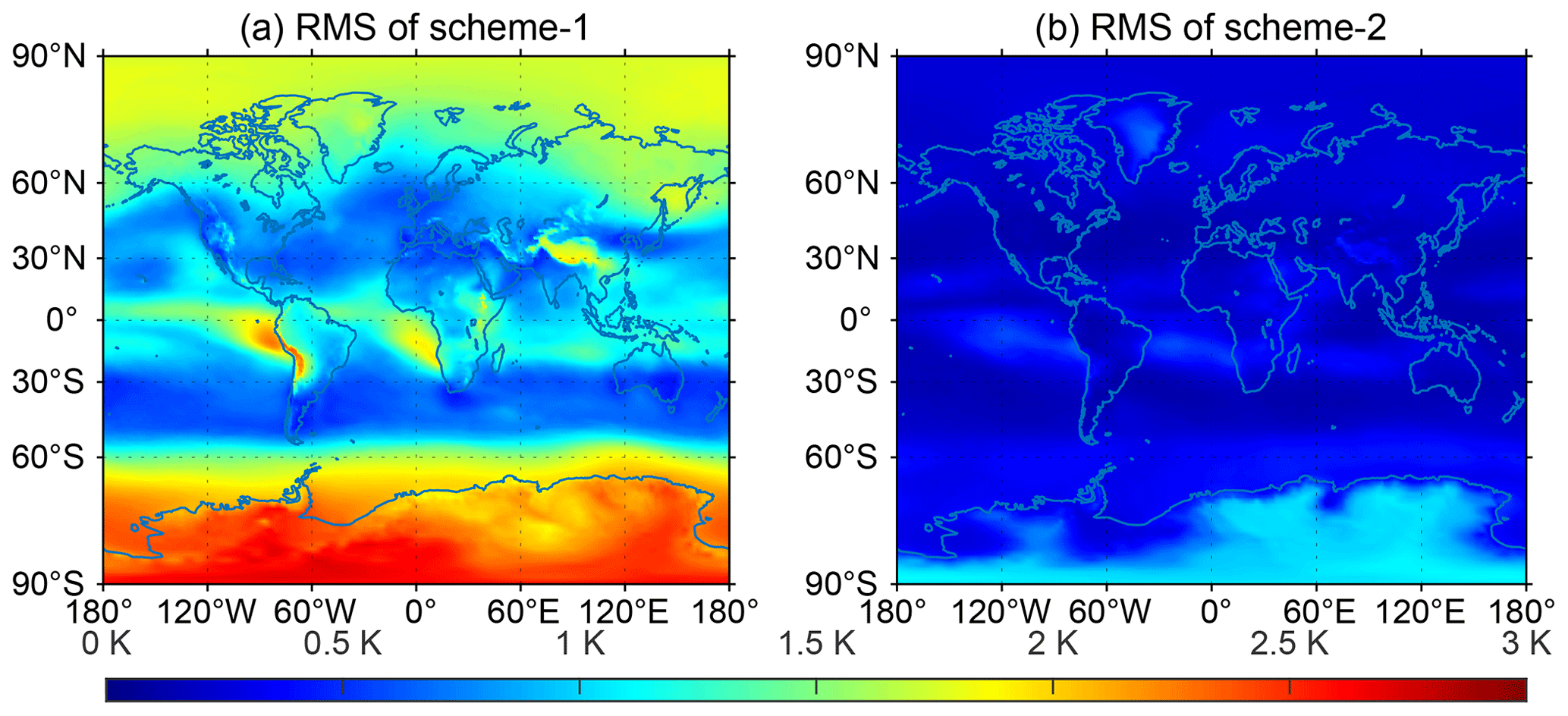
Figure 2 Mean of rms's of the T_m residuals of 120 monthly mean profiles from the 10-year period at each grid point for scheme 1 (a, for linear function) and scheme 2 (b, for three-order polynomial function).

2 Methodology for new model construction

2.1 Data source

ERA5 reanalysis data were the latest reanalysis data developed by the ECMWF. In this research, ERA5 monthly mean reanalysis data in the 10-year period from 2008 to 2017 containing geopotential heights, temperatures, and specific humidity at 37 pressure levels with a horizontal resolution of 1^∘ × 1^∘ were downloaded from the web server of the Copernicus Climate Change Service (C3S). The geopotential heights, which are often used in meteorology, were then converted to WGS-84 ellipsoidal heights. Water vapor pressure was calculated by (Nafisi et al., 2012)

$$\begin{array}{}\text{(4)}& e=qp/(\mathrm{0.622}+\mathrm{0.378}q),\end{array}$$

where q is the specific humidity, which can be obtained from NWM data; p is the atmospheric pressure.

2.2 Vertical variation in T_m

The ERA5 monthly mean products were used to analyze the vertical variation in T_m. As defined in Eq. (3), T_m is a function of water vapor pressure and temperature. The variation in water vapor pressure in the vertical direction has been known to be nonlinear, while the vertical variation in temperature is often assumed to be a linear decay function (Dousa and Elias, 2014). In fact, there is such a phenomenon that temperature increases with the increase in height, the so-called temperature inversion, which occurs in both the upper atmosphere and near ground surface, meaning that the vertical variation in temperature is complex. As a result, T_m in the vertical direction varies nonlinearly due to the irregular variations in both water vapor pressure and temperature in the vertical direction. Figure 1 shows four vertical profiles of water vapor pressure, temperature, and T_m at the pressure levels that were under a 10 km ellipsoidal height at four grid points obtained from ERA5 monthly mean reanalysis in December 2017. It should be noted that the surface heights of the four grid points were different, and they were 0, 301, 13, and 180 m, respectively. Panels (a) and (b) show that, in the height range near the surface, temperature increases with the increase in height. In addition, all the four T_m profiles (the black curves with dots) in these panels show a nonlinear variation trend. This implies that using a constant lapse rate to model the vertical T_m variation trend will result in large errors; i.e., the T_m profiles cannot be accurately modeled through a constant T_m lapse rate. This finding aligns well with that of other researchers (e.g., Yao et al., 2018).

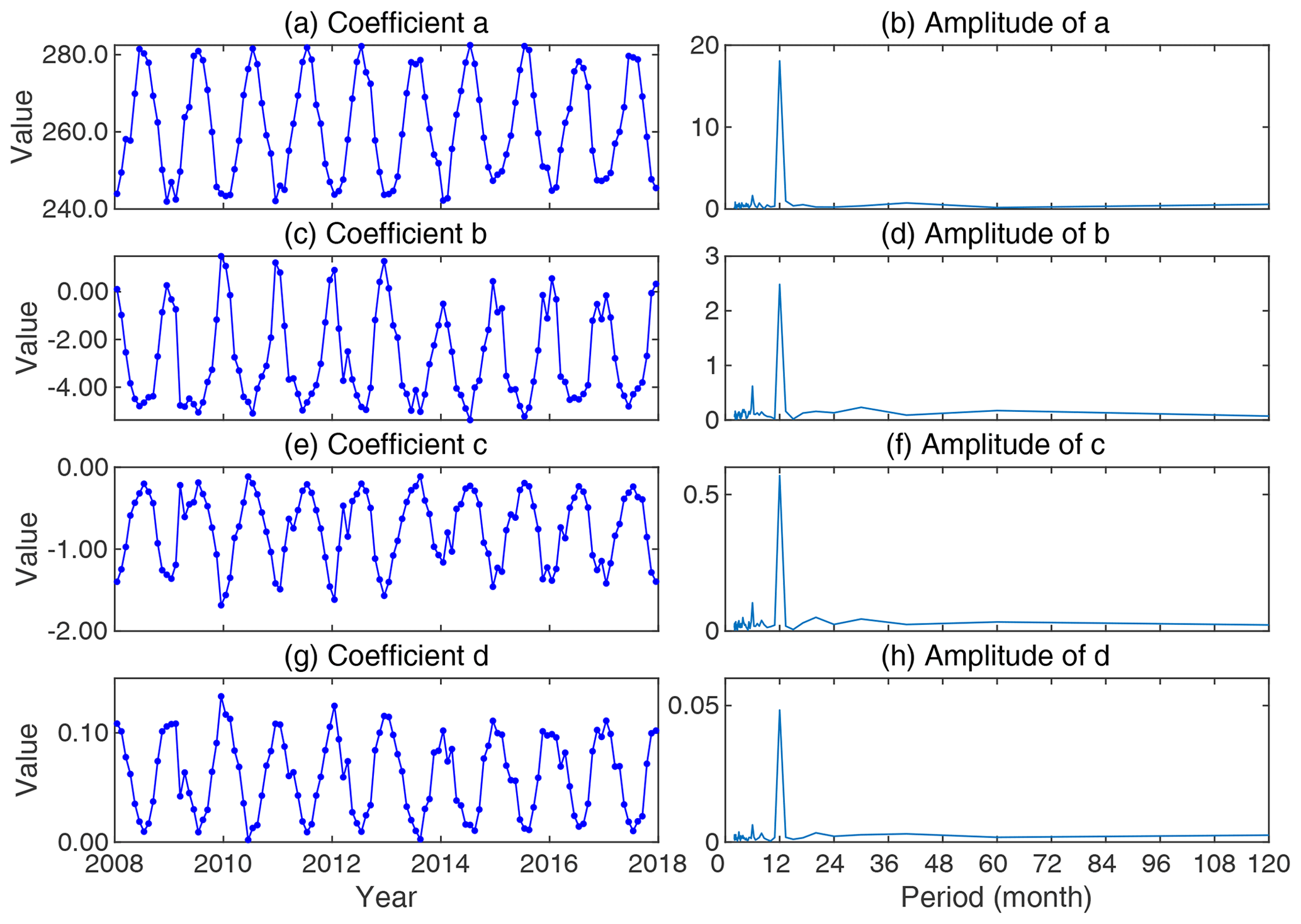
Figure 3 Periodicity reflected in the 10-year time series of each coefficient in the three-order polynomial function at 60^∘ N, 120^∘ E.

2.3 Three-order polynomial function for T_m vertical fitting

A linear T_m decay function with a constant T_m lapse rate can be expressed as

$$\begin{array}{}\text{(5)}& T_{\mathrm{m}}=\mathit{\alpha }+\mathit{\beta }(H-h_{\mathrm{0}}),\end{array}$$

where α is the T_m value at the reference height h₀; β is the T_m lapse rate and H is the ellipsoidal height (km) of the user site. An equivalent expression of Eq. (5) is

$$\begin{array}{}\text{(6)}& T_{\mathrm{m}}={\mathit{\alpha }}^{\prime }+{\mathit{\beta }}^{\prime }H,\end{array}$$

where α^′ denotes the T_m value at 0 km ellipsoidal height. Some T_m models were constructed based on this linear T_m decay function. T_m values from different height ranges can be used to calculate the T_m lapse rate. However, if T_m varies nonlinearly in the vertical direction, the calculated T_m lapse-rate values would have large errors. To overcome this problem, in this research, a three-order polynomial function was selected for a new T_m model:

$$\begin{array}{}\text{(7)}& T_{\mathrm{m}}=a+bH+c{H}^{\mathrm{2}}+d{H}^{\mathrm{3}},\end{array}$$

where $a,b,c,d$ are the four unknown coefficient parameters of the fitting function.

For the estimation of the two sets of unknown coefficient parameters expressed in Eqs. (6) and (7), two schemes, named scheme 1 and scheme 2, fitted the sample data of T_m profiles of the 120 monthly mean reanalysis data over the 10-year period from 2008 to 2017 at each grid point for the two functions. It should be noted that only those T_m values from heights under 10 km were selected for the sample data. For measuring how well the fitting function fits the sample data, the root mean square (rms) of the differences between the T_m values resulting from the fitting function and the sample data was calculated by

$$\begin{array}{}\text{(8)}& \mathrm{rms}=\sqrt{{\displaystyle \frac{\mathrm{1}}{n}}\sum _i^n{\mathrm{\Delta }}_i^{\mathrm{2}}},\end{array}$$

where Δ_i is the residual of T_m at the ith pressure level over the grid point. Figure 2 shows the map for the mean of the rms's of the fitting residuals of the T_m from the aforementioned 120 monthly mean T_m profiles (the samples) at each of the grid points. The mean of the mean rms's at all global grid points for scheme 1 and scheme 2 were 1.26 and 0.30 K, respectively. In addition, the rms results in panel (a) (for linear function) were latitude-dependent, and small rms's (blue) were in midlatitude regions; large rms values in both panels were in Antarctica. Comparing the two panels, we found that the rms values shown in panel (b) were all very small and significantly smaller than those of panel (a), meaning that the three-order polynomial fitting function was superior to the linear fitting function.

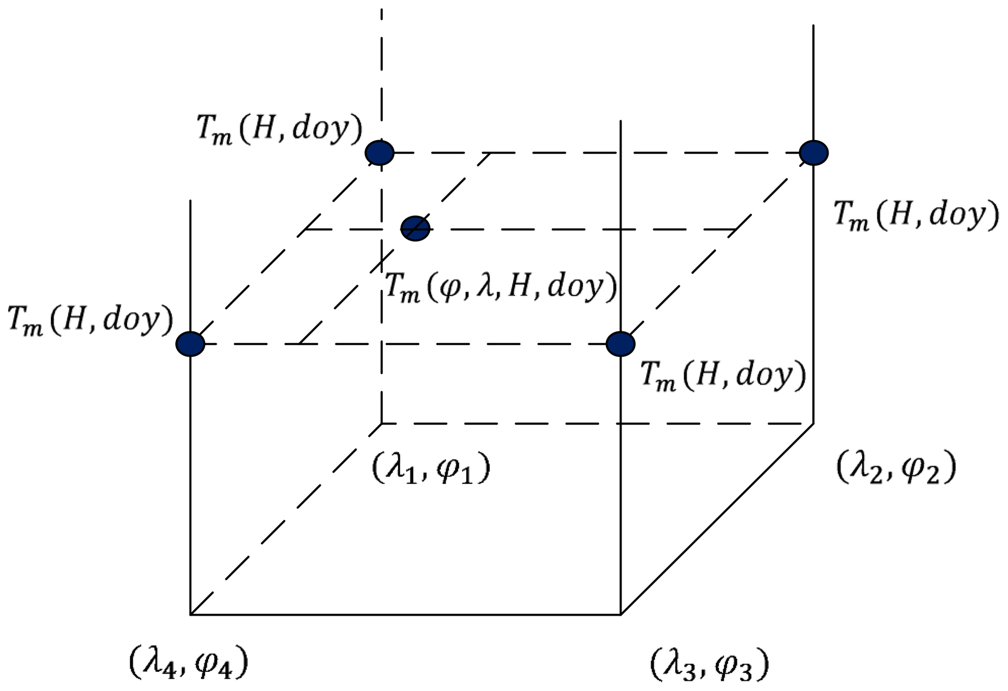
Figure 4 Spatial interpolation of the T_m value for the target point (φλH). After obtaining the T_m values at height H at the four grid points (see the four grids on the top plane) by the GGNTm model using Eq. (7), the T_m value at the target point can be interpolated (the dashed rectangle).

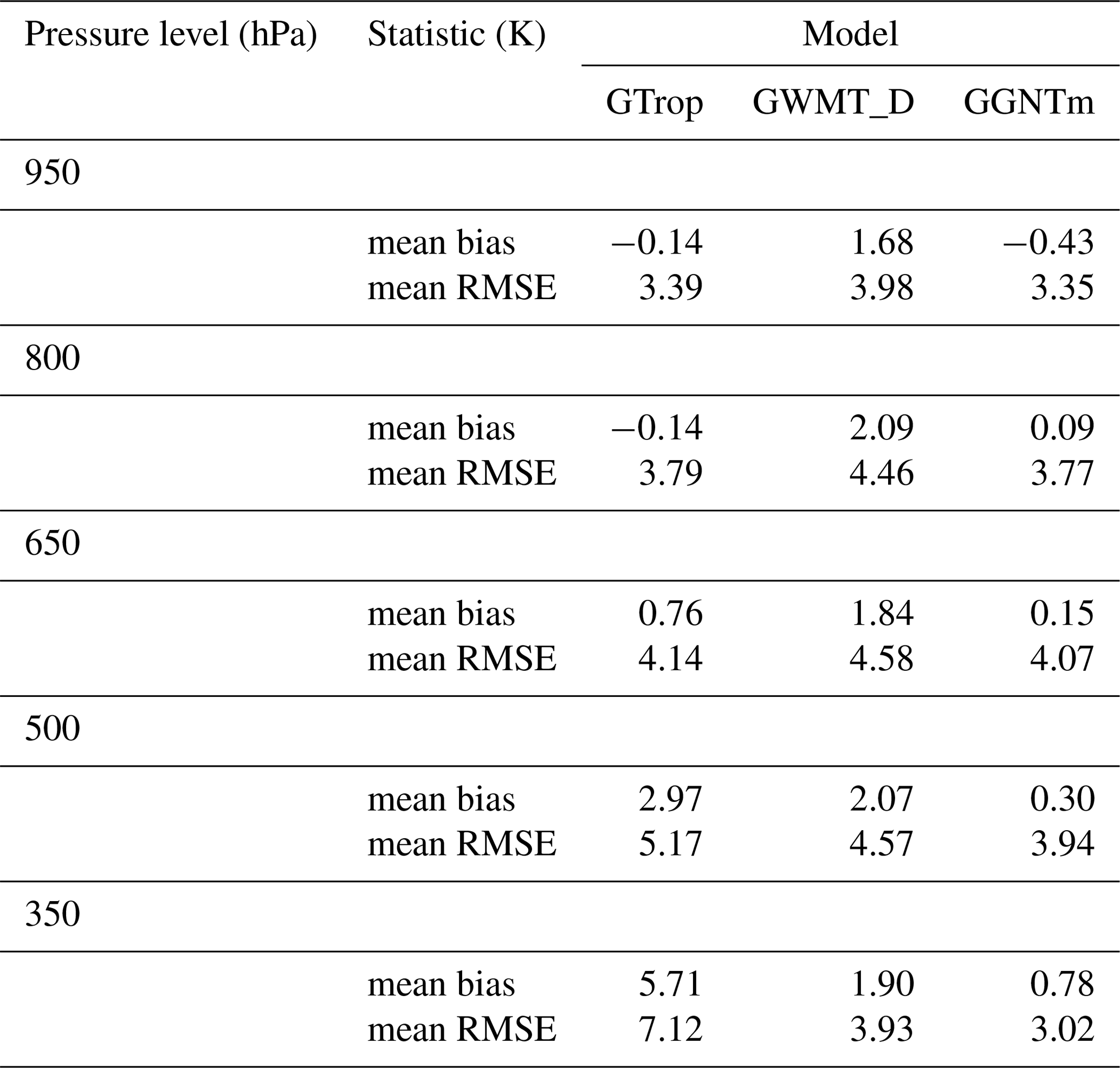
Table 1 Mean bias and mean RMSE of T_m values at each of five pressure levels at 12:00 UTC at all global grid points in 2018 resulting from each of the three models selected.

2.4 T_m temporal fitting for the new model

In the previous section, the 10-year time series of coefficients in the three-order polynomial function expressed in Eq. (7) at each of the grid points were obtained from the least-squares estimation. Since they were not constant values, the temporal variation in each coefficient at each grid point needs to be further modeled for the new grid-based empirical T_m model proposed in this study, GGNTm. The seasonal variation reflected in the 10-year time series of each of the coefficients $r=a,b,c,d$ was analyzed using the fast Fourier transform (FFT), and results for seasonality and periodicity at point 60^∘ N, 120^∘ E are shown in Fig. 3, which presented noticeable annual and semi-annual amplitudes. Similar periodicities were also found at other grid points. According to these characteristics, the fitting model for GGNTm containing three terms including mean, annual, and semi-annual amplitudes for each coefficient time series at each grid point expressed by the following was adopted in this study:

$$\begin{array}{}\text{(9)}& r=A_{\mathrm{0}}+A_{\mathrm{1}}\cos \left({\displaystyle \frac{\mathrm{doy}-d_{\mathrm{1}}}{\mathrm{365.25}}}\mathrm{2}\mathit{\pi }\right)+A_{\mathrm{2}}\cos \left({\displaystyle \frac{\mathrm{doy}-d_{\mathrm{2}}}{\mathrm{365.25}}}\mathrm{4}\mathit{\pi }\right),\end{array}$$

where A₀, A₁, and A₂ are the mean, annual, and semi-annual amplitudes, respectively; doy denotes “day of year”; d₁ and d₂ are the initial phases of the annual and semi-annual periodicities, which are estimated together with the mean and amplitudes.

Then, the mean, annual, and semi-annual amplitudes and initial phases for each coefficient at each of the grid points over the globe (with the resolution of 1^∘ × 1^∘ ) were determined using the least-squares estimation method and the 10-year time series of the coefficient. To calculate T_m for a specific site and time, e.g., for a GNSS station at an observing time, the following three-step procedure needs to be carried out:

1. use Eq. (9) to calculate each of the four coefficients at each of the four grid points surrounding the user site;

2. use Eq. (7) to calculate the T_m values at the height of the user site at each of the above four grid points (which is for the height dimension);

3. use an interpolation method, such as the inverse distance weighting or bilinear interpolation, on the four T_m values from step (2) to obtain the T_m value for the user site (which is for the horizontal dimension, as shown in Fig. 4).

Till now the new model has been developed based on the 10-year sample data from 2008 to 2017. This model will be validated using the model-predicted T_m results in 2018 compared against the same year's (i.e., out-of-sample) reference data. Results will be discussed in the next section.

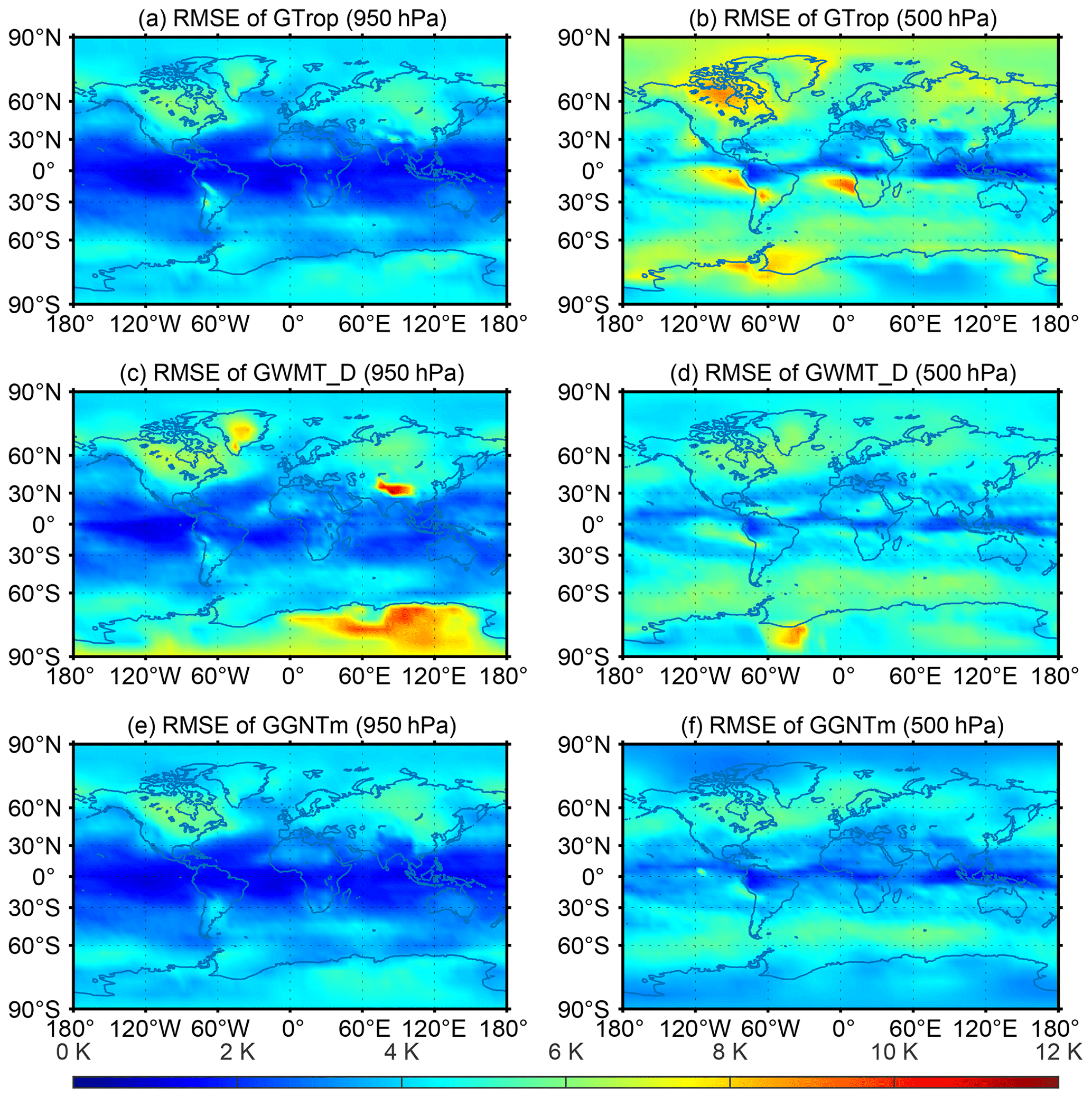
Figure 5 RMSE of T_m at each grid point at 950 hPa (a, c, e) and 500 hPa (b, d, f) pressure levels in 2018 resulting from GTrop, GWMT_D, and GGNTm.

3 Evaluation of GGNTm

For the performance assessment of our newly developed T_m model, T_m values over different pressure levels obtained from both ERA-5 hourly reanalysis (at 12:00 UTC) and globally distributed radiosonde profiles in 2018 were selected as the references. Thus, both 24 and 12 h variations in T_m have been contained in the reference data for the evaluation of our new model. The two statistics – bias and RMSE – were utilized to measure the systematic discrepancy and the accuracy of the model results. Their formulas are

$$\begin{array}{}\text{(10)}& {\displaystyle }\mathrm{bias}={\displaystyle \frac{\mathrm{1}}{n}}\sum _{i=\mathrm{1}}^n(T_{{\mathrm{m}}_i}^{\mathrm{model}}-T_{{\mathrm{m}}_i}^{\mathrm{ref}}),\text{(11)}& {\displaystyle }\mathrm{RMSE}=\sqrt{{\displaystyle \frac{\mathrm{1}}{n}}\sum _{i=\mathrm{1}}^n(T_{{\mathrm{m}}_i}^{\mathrm{model}}-T_{{\mathrm{m}}_i}^{\mathrm{ref}}{)}^{\mathrm{2}}},\end{array}$$

where i is the index of the data element; $T_{{\mathrm{m}}_i}^{\mathrm{model}}$ denotes the model resultant T_m value; $T_{{\mathrm{m}}_i}^{\mathrm{ref}}$ denotes the reference T_m value; n is the number of the T_m values in the statistics.

3.1 Comparison with ERA5 hourly data

As the first set of the reference selected for the evaluation of the new model, ERA-5 hourly data (with the resolution of 5^∘ × 5^∘) at 12:00 UTC on each day in 2018, which were out-of-sample data, were downloaded from the C3S. Then they were converted to T_m profiles and T_m values at each of five pressure levels: 950, 800, 650, 500, and 350 hPa were used to calculate the bias and RMSE of the new model's T_m results at the pressure level. In addition to the GGNTm model, the other two empirical models developed in recent years including GTrop and GWMT_D, in which different vertical correction methods were also applied, were also evaluated for performance comparisons of GGNTm and these two models.

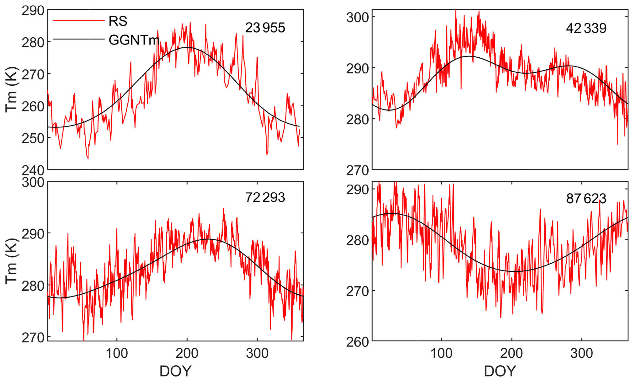
Figure 6 T_m values (at the earth surface) integrated from the radiosonde measurements as well as that predicted by GGNTm at each of the four radiosonde stations (nos. 23955, 42339,72293, and 87623).

Table 1 shows the mean bias and mean RMSE of the T_m values over all global grid points resulting from each of the above three models. As we can see, on a global scale, GGNTm outperformed all the other two models, especially at high pressure levels. The GTrop has been proved to be considerably better than GPT3 (Sun et al., 2019), owing to its use of the T_m lapse rate, although its T_m results still had large errors at high pressure levels, which is most likely to result from neglecting the nonlinear vertical variation in T_m. The large bias and RMSE of the GWMT_D results were possibly because its modeling was based on NCEP reanalysis data, and there may exist differences between the reanalysis data from ECMWF and NCEP (Chen et al., 2011; Decker et al., 2012). Compared to GTrop and GWMT_D, GGNTm performed very well at all pressure levels. This is because the model accounted for the vertical nonlinear variation in T_m.

The results shown in Table 1 were the statistics of all global grid points at each of the five pressure levels selected. For more refined results, Fig. 5 shows the map for the RMSE of T_m at each grid point at either the 950 or 500 hPa pressure levels resulting from three models. The 950 hPa pressure level (Fig. 5a, c, e) results indicated that the RMSEs of T_m resulting from all the three models were latitude-dependent and high-accuracy T_m values (in blue) were mainly in low-latitude belts. However, the results at the 500 hPa pressure level (Fig. 5b, d, f) indicated that the new model significantly outperformed the other two models. In addition, from the 950 hPa pressure level results, the percentages of those RMSE values that were under 5 K from all the global grid points for GTrop, GWMT_D, and GGNTm were 93.4 %, 82.1 %, and 94.6 %, respectively; while the corresponding percentage values at the 500 hPa level were 44.9 %, 70.6 %, and 88.7 %. These suggest that larger improvements made by the new model, i.e., GGNTm, over the other two models were at high-altitude pressure levels.

3.2 Comparison with radiosonde data

In this section, T_m from radiosonde profiles were used as the reference for the performance assessment of the models selected. The original radiosonde data at all globally distributed stations in 2018 were downloaded from the website of the University of Wyoming (http://weather.uwyo.edu/upperair/, last access: 13 March 2020). Different from the use of reanalysis data as the reference, water vapor pressure at each pressure level from a radiosonde profile was calculated through a mixing ratio:

$$\begin{array}{}\text{(12)}& e=Rp/(\mathrm{622}+R),\end{array}$$

where R denotes the mixing ratio (g/kg).

Table 2 Mean bias and mean RMSE of T_m values at 428 globally distributed radiosonde stations in 2018 resulting from GPT3, GTrop, GWMT_D, and GGNTm.

Note: the values within square brackets are the minimum and maximum.

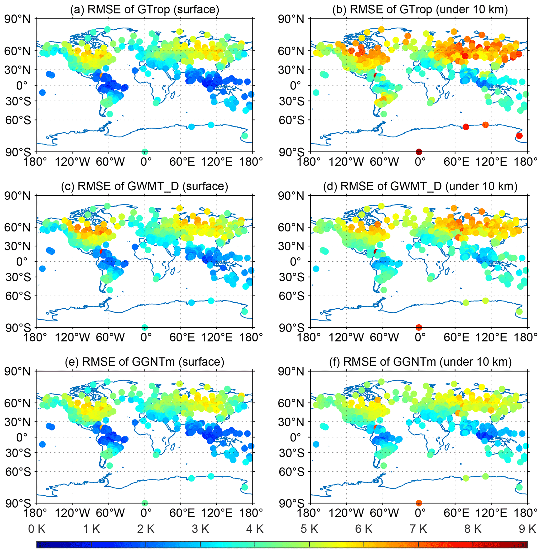
Figure 7 RMSE of T_m at surface level (a, c, e) and all pressure levels under 10 km (b, d, f) at each of the 428 radiosonde stations in 2018 resulting from GTrop, GWMT_D, and GGNTm. The RMSE of T_m under 10 km was calculated using the differences between model-predicted T_m values and the T_m values over all pressure levels with a height of less than 10 km.

An additional data pre-processing procedure needs to be conducted for data quality control. Those poor radiosonde profiles needed to be identified and excluded from their use for the reference. The first check was for a valid mixing ratio value: if a pressure level lacks a valid mixing ratio value, then it is regarded as invalid and thus to be excluded. After this initial checking was performed, further identifications were also carried out. A profile would be excluded if it met any one of the following four conditions:

1. the profile lacks surface meteorological observations;

2. the pressure value of the top pressure level is greater than 100 hPa;

3. the difference in the pressure values at two successive levels is under 200 hPa;

4. the profile consists of a few pressure levels; e.g., if $\mathrm{\Delta }P/n\le \mathrm{30}$ hPa (where ΔP is the difference of the pressure values at the surface and the 100 hPa pressure levels and n is the number of all pressure levels from the surface to the 100 hPa pressure levels), then the profile was regarded to have sufficient number of pressure levels; otherwise it would be excluded from the use in the testing.

Sounding balloons are commonly launched twice a day (at 00:00 and 12:00 UTC). In this research, only those stations that had at least 300 profiles in 2018 were selected in the model performance assessment. After the above five-step quality control procedure was performed, a total of 260 140 profiles from 428 global radiosonde stations were finally used in the performance evaluation of three selected models. Figure 6 shows the T_m values (at the earth surface) integrated from the radiosonde measurements as well as that predicted by GGNTm at four radiosonde stations.

Table 2 shows the mean bias and RMSE of surface T_m values and T_m values at all pressure levels from the surface to 10 km height at all the aforementioned radiosonde stations resulting from each of the three models that were the same as the ones tested in the previous section. For the surface T_m results, the mean RMSE of GTrop and GGNTm were very close; GWMT_D was the worst, with the largest bias and RMSE values, which may be due to its low horizontal resolution (5^∘ × 5^∘). The other set of results, the RMSE of T_m under 10 km, was calculated using the differences between model-predicted T_m values and the reference T_m values over all pressure levels with a height of less than 10 km. A small RMSE of T_m under 10 km indicates that the model performs well at any altitudes below the tropopause. As we can see, GWMT_D was slightly better than GTrop, possibly because the T_m value from the former was interpolated from the T_m values at four height levels; the mean bias of T_m from the new model, GGNTm, was the lowest, with the value of −0.16, which was close to 0, meaning nearly unbiased; the RMSE of the new model was also the lowest, among the three models, which suggests that the vertical nonlinear variation in T_m was modeled more accurately in the new model than in the other existing models.

Similar to Fig. 5, Fig. 7 shows the map for the RMSE of T_m values at each of the 428 radiosonde stations in 2018 at the surface pressure level (Fig. 5a, c, e) and all pressure levels with a height of less than 10 km (Fig. b, d, f) resulting from GTrop, GWMT_D, and GGNTm. It can be found that the RMSEs of all models were latitude-dependent, and those stations that had a large RMSE value were mostly located in north Africa and northeast America. At the four stations located in Antarctic, their surface T_m values were accurately modeled by these models. However, in terms of the RMSE of all pressure levels under 10 km, the GTrop results were relatively large at the four stations, whilst both GWMT_D and GGNTm performed well at three of the stations.

To further evaluate the performance of the three models at different height ranges under 10 km, the models' T_m values from the aforementioned radiosonde profiles at the 428 global stations were divided into five height ranges, and Fig. 8 shows each height range's bias and RMSE. We can see the following results: (1) in the height ranges above 4 km, the GTrop results had the largest bias and largest RMSE, and GWMT_D was considerably better than GTrop; (2) in low height ranges the GWMT_D results were the worst; (3) in all height ranges the GGNTm results were nearly unbiased and their accuracy varied little with height. The GGNTm model's consistent high accuracy in all height ranges suggests that the characteristics of the vertical nonlinear variation in T_m are modeled by the proposed model more accurately than the other models.

Figure 8 Bias and RMSE of T_m from radiosonde profiles at 428 global radiosonde stations in each of five height ranges resulting from GTrop, GWMT_D, and GGNTm.

3.3 Evaluation of GGNTm under extreme weather conditions

The performance of our model under extreme weather conditions has also been assessed. The T_m values integrated from the radiosonde profiles at KingsPark radiosonde station (no. 45005, Hong Kong) from August to September in 2018 (summer storm period) were taken as the reference data in this research. As is shown in Fig. 9, the T_m values at the station predicted by GGNTm as well as a T_m–T_s model ($T_{\mathrm{m}}=\mathrm{0.6195}\times T_{\mathrm{s}}+\mathrm{103.3452}$) developed using T_m and T_s series at KingsPark station (He et al., 2019) were compared against corresponding radiosonde measurements during the summer storm period. The daily total rainfall data (published by Hong Kong Observatory, https://www.hko.gov.hk, last access: 2 December 2020) during the 2 months are also shown in the figure. Heavy rainfall occurred frequently in Hong Kong during the 2 months, and a super typhoon, named Mangkhut, landed near Hong Kong and caused torrential rain on 16 September. As is shown in the figure, our model shows clear outperformance during the 2 months compared to the T_m–T_s model. More experiments showed that the coefficients of T_m–T_s models vary significantly with time (i.e., 0.6195 vs. 0.58 for the linear part and 103.3452 vs. 115.71 for the constant part, respectively), which means that a T_m−T_s model that is based on the linear regression may have large errors during some periods.

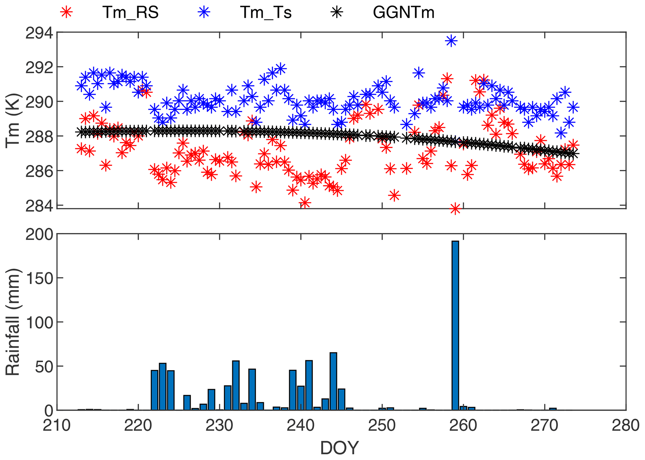
Figure 9 T_m derived from radiosonde profiles, the T_m−T_s model, GGNTm from August to September in 2018 at KingsPark station, and the daily total rainfall at Hong Kong International Airport.

3.4 Impact of GGNTm on PWV

The accuracy of GNSS-PWV over a GNSS site at an observing time is dependent upon the accuracies of the ZWD and the conversion factor. Uncertainty analysis has been conducted by some researchers to study the uncertainty of the GNSS-derived PWV resulting from different variables, including the uncertainty of GNSS-ZTD, the atmospheric pressure, the T_m, and other constants utilized (Jiang et al., 2019b; Ning et al., 2016). This section mainly focuses on the impact of the newly developed T_m model on PWV; however, it is difficult to evaluate the impact of T_m on the GNSS-PWV directly. In this research, the ZWD and T_m derived from the ERA5 hourly reanalysis (the same as the data utilized in Sect. 3.1) were used for simulating the GNSS-PWV sensing. The ZWDs at each of the pressure levels over the globally distributed grid points (2664 grid points in total) were calculated through integration:

$$\begin{array}{}\text{(13)}& \mathrm{ZWD}={\mathrm{10}}^{-\mathrm{6}}{\int }_H^{\mathrm{\infty }}(k_{\mathrm{2}}^{\prime }{\displaystyle \frac{e}{T}}+k_{\mathrm{3}}{\displaystyle \frac{e}{T^{\mathrm{2}}}})\mathrm{d}h,\end{array}$$

where H is the height of the reference pressure level. Then the reference PWVs can be obtained using the ZWDs and the corresponding conversion factors resulting from the reference T_m values, as is shown in Eq. (1). Similarly, the PWVs resulting from different empirical T_m models can be obtained. The statistical results of the RMSEs of the PWVs resulting from different model-predicted T_m values by comparing the PWVs resulting from the reference T_m values (as references) are shown in Fig. 10. As we can see, the performance of both GGNTm and GTrop were better than GWMT_D. The mean RMSE of the predicted PWVs resulting from GTrop and GGNTm over 2664 grid points were approximately the same. But the maximum RMSE of the PWVs resulting from GGNTm were better than GTrop from 1000 to 775 hPa. This is because the nonlinear variation in T_m in the vertical direction was properly modeled in some regions. We can also find that there are not significant differences between the RMSEs of the predicted PWVs resulting from GGNTm and GTrop due to less water vapor at the pressure levels with high altitudes, although the accuracy of the model-predicted T_m values resulting from GGNTm was better than GTrop. However, due to the fact that the water vapor content varies with latitude, terrain, season, and weather, the improvement in the model-predicted T_m values at pressure levels with high altitudes is still meaningful.

Figure 10 Mean RMSE and maximum RMSE of PWV values at each of the pressure levels at 12:00 UTC at all global grid points in 2018 resulting from each of the three models selected.

4 Conclusions

In GNSS meteorology, T_m is an essential parameter for converting GNSS-ZWD to PWV over the GNSS observing station. In practice, the T_m value over a GNSS station at an observing time is commonly obtained from an empirical T_m model, such as GPT3, GTrop, and GWMT_D. In this research, a new global gridded empirical T_m model, named GGNTm, was developed. In this model, the vertical nonlinear variation in T_m was modeled using a three-order polynomial function fitting ERA5 monthly mean reanalysis data over the 10-year period from 2008 to 2017; and seasonal variation terms, including mean, annual, and semi-annual amplitudes, for each of the coefficients in the polynomial function at each of global grid points were also modeled based on the 10-year time series of the coefficient.

The performance of the newly developed GGNTm model was assessed and compared with GTrop and GWMT using model-predicted T_m values in 2018 against two references in the same year: (1) T_m from ERA5 hourly reanalysis data and (2) T_m from radiosonde profiles at 428 global radiosonde stations. Compared to the first reference, the RMSEs of T_m values resulting from GGNTm at five pressure levels over all the global grid points in 2018 were significantly smaller than those of the other three models at high-altitude pressure levels. Compared to the second reference, the mean bias and mean RMSE of T_m resulting from GGNTm at all the 428 radiosonde stations in 2018 were ­0.34 and 3.89 K, respectively; and the mean bias and mean RMSE of T_m resulting from GGNTm at all pressure levels from the surface to 10 km height were ­0.16 and 4.20 K, respectively, which was significantly smaller than those of all the other three models. In all five height ranges from the surface to 10 km in altitude, the GGNTm results were nearly unbiased, and their accuracy varied little with height. This result suggests that the characteristics of the vertical nonlinear variation in T_m is modeled by the approach proposed in this study more accurately than the existing models. In addition, the impact of GGNTm on GNSS-PWV was analyzed. The results showed that the accuracy of the PWV resulting from GGNTm outperformed the GTrop and GWMT models.

The improvement in the accuracy of the new T_m model has significance for both long-term GNSS-PWV analysis and NRT/RT GNSS-PWV sensing. Our future work will be focusing on using high temporal-resolution atmospheric data such as ERA5 hourly reanalysis data, instead of monthly mean data used in this study, to model the temporal variation in the coefficients in the T_m fitting function for further improving the accuracy of the GGNTm model.