the Creative Commons Attribution 4.0 License.
the Creative Commons Attribution 4.0 License.
 | 04 Jan 2021
Robust statistical calibration and characterization of portable low-cost air quality monitoring sensors to quantify real-time O3 and NO2 concentrations in diverse environments
Ravi Sahu
Ayush Nagal
Kuldeep Kumar Dixit
Harshavardhan Unnibhavi
Srikanth Mantravadi
Srijith Nair
Yogesh Simmhan
Brijesh Mishra
Rajesh Zele
Ronak Sutaria
Vidyanand Motiram Motghare
Purushottam Kar
Low-cost sensors offer an attractive solution to the challenge of establishing affordable and dense spatio-temporal air quality monitoring networks with greater mobility and lower maintenance costs. These low-cost sensors offer reasonably consistent measurements but require in-field calibration to improve agreement with regulatory instruments. In this paper, we report the results of a deployment and calibration study on a network of six air quality monitoring devices built using the Alphasense O3 (OX-B431) and NO2 (NO2-B43F) electrochemical gas sensors. The sensors were deployed in two phases over a period of 3 months at sites situated within two megacities with diverse geographical, meteorological and air quality parameters. A unique feature of our deployment is a swap-out experiment wherein three of these sensors were relocated to different sites in the two phases. This gives us a unique opportunity to study the effect of seasonal, as well as geographical, variations on calibration performance. We report an extensive study of more than a dozen parametric and non-parametric calibration algorithms. We propose a novel local non-parametric calibration algorithm based on metric learning that offers, across deployment sites and phases, an R2 coefficient of up to 0.923 with respect to reference values for O3 calibration and up to 0.819 for NO2 calibration. This represents a 4–20 percentage point increase in terms of R2 values offered by classical non-parametric methods. We also offer a critical analysis of the effect of various data preparation and model design choices on calibration performance. The key recommendations emerging out of this study include (1) incorporating ambient relative humidity and temperature into calibration models; (2) assessing the relative importance of various features with respect to the calibration task at hand, by using an appropriate feature-weighing or metric-learning technique; (3) using local calibration techniques such as k nearest neighbors (KNN); (4) performing temporal smoothing over raw time series data but being careful not to do so too aggressively; and (5) making all efforts to ensure that data with enough diversity are demonstrated in the calibration algorithm while training to ensure good generalization. These results offer insights into the strengths and limitations of these sensors and offer an encouraging opportunity to use them to supplement and densify compliance regulatory monitoring networks.
- Article
(4654 KB) - Full-text XML
-
Supplement
(1028 KB) - BibTeX
- EndNote


Elevated levels of air pollutants have a detrimental impact on human health as well as on the economy (Chowdhury et al., 2018; Landrigan et al., 2018). For instance, high levels of ground-level O3 have been linked to difficulty in breathing, increased frequency of asthma attacks and chronic obstructive pulmonary disease (COPD). The World Health Organization reported (WHO, 2018) that in 2016, 4.2 million premature deaths worldwide could be attributed to outdoor air pollution, 91 % of which occurred in low- and middle-income countries where air pollution levels often did not meet its guidelines. There is a need for accurate real-time monitoring of air pollution levels with dense spatio-temporal coverage.
Existing regulatory techniques for assessing urban air quality (AQ) rely on a small network of Continuous Ambient Air Quality Monitoring Stations (CAAQMSs) that are instrumented with accurate air quality monitoring gas analyzers and beta-attenuation monitors and provide highly accurate measurements (Snyder et al., 2013; Malings et al., 2019). However, these networks are established at a commensurately high setup cost and are cumbersome to maintain (Sahu et al., 2020), making dense CAAQMS networks impractical. Consequently, the AQ data offered by these sparse networks, however accurate, limit the ability to formulate effective AQ strategies (Garaga et al., 2018; Fung, 2019).
In recent years, the availability of low-cost AQ (LCAQ) monitoring devices has provided exciting opportunities for finer-spatial-resolution data (Rai et al., 2017; Baron and Saffell, 2017; Kumar et al., 2015; Schneider et al., 2017; Zheng et al., 2019). The cost of a CAAQMS system that meets federal reference method (FRM) standards is around USD 200 000, while that of an LCAQ device running commodity sensors is under USD 500 (Jiao et al., 2016; Simmhan et al., 2019). In this paper, we use the term “commodity” to refer to sensors or devices that are not custom built and instead sourced from commercially available options. The increasing prevalence of the Internet of things (IoT) infrastructure allows for building large-scale networks of LCAQ devices (Baron and Saffell, 2017; Castell et al., 2017; Arroyo et al., 2019).
Dense LCAQ networks can complement CAAQMSs to help regulatory bodies identify sources of pollution and formulate effective policies; allow scientists to model interactions between climate change and pollution (Hagan et al., 2019); allow citizens to make informed decisions, e.g., about their commute (Apte et al., 2017; Rai et al., 2017); and encourage active participation in citizen science initiatives (Gabrys et al., 2016; Commodore et al., 2017; Gillooly et al., 2019; Popoola et al., 2018).
1.1 Challenges in low-cost sensor calibration
Measuring ground-level O3 and NO2 is challenging as they occur at parts-per-billion levels and intermix with other pollutants (Spinelle et al., 2017). LCAQ sensors are not designed to meet rigid performance standards and may generate less accurate data as compared to regulatory-grade CAAQMSs (Mueller et al., 2017; Snyder et al., 2013; Miskell et al., 2018). Most LCAQ gas sensors are based on either metal oxide (MOx) or electrochemical (EC) technologies (Pang et al., 2017; Hagan et al., 2019). These present challenges in terms of sensitivity towards environmental conditions and cross-sensitivity (Zimmerman et al., 2018; Lewis and Edwards, 2016). For example, O3 electrochemical sensors undergo redox reactions in the presence of NO2. The sensors also exhibit loss of consistency or drift over time. For instance, in EC sensors, reagents are spent over time and have a typical lifespan of 1 to 2 years (Masson et al., 2015; Jiao et al., 2016). Thus, there is a need for the reliable calibration of LCAQ sensors to satisfy performance demands of end-use applications (De Vito et al., 2018; Akasiadis et al., 2019; Williams, 2019).
1.2 Related works
Recent works have shown that LCAQ sensor calibration can be achieved by co-locating the sensors with regulatory-grade reference monitors and using various calibration models (De Vito et al., 2018; Hagan et al., 2019; Morawska et al., 2018). Zheng et al. (2019) considered the problem of dynamic PM2.5 sensor calibration within a sensor network. For the case of SO2 sensor calibration, Hagan et al. (2019) observed that parametric models such as linear least-squares regression (LS) could extrapolate to wider concentration ranges, at which non-parametric regression models may struggle. However, LS does not correct for (non-linear) dependence on temperature (T) or relative humidity (RH), for which non-parametric models may be more effective.
Since electrochemical sensors are configured to have diffusion-limited responses and the diffusion coefficients could be affected by ambient temperature, Sharma et al. (2019), Hitchman et al. (1997) and Masson et al. (2015) found that at RH exceeding 75 % there is substantial error, possibly due to condensation on the potentiostat electronics. Simmhan et al. (2019) used non-parametric approaches such as regression trees along with data aggregated from multiple co-located sensors to demonstrate the effect of the training dataset on calibration performance. Esposito et al. (2016) made use of neural networks and demonstrated good calibration performance (with mean absolute error <2 ppb) for the calibration of NO2 sensors. However, a similar performance was not observed for O3 calibration. Notably, existing works mostly use a localized deployment of a small number of sensors, e.g., Cross et al. (2017), who tested two devices, each containing one sensor per pollutant.
1.3 Our contributions and the SATVAM initiative
The SATVAM (Streaming Analytics over Temporal Variables from Air quality Monitoring) initiative has been developing low-cost air quality (LCAQ) sensor networks based on highly portable IoT software platforms. These LCAQ devices include (see Fig. 3) PM2.5 as well as gas sensors. Details on the IoT software platform and SATVAM node cyber infrastructure are available in Simmhan et al. (2019). The focus of this paper is to build accurate and robust calibration models for the NO2 and O3 gas sensors present in SATVAM devices. Our contributions are summarized below:
-
We report the results of a deployment and calibration study involving six sensors deployed at two sites over two phases with vastly different meteorological, geographical and air quality parameters.
-
A unique feature of our deployment is a swap-out experiment wherein three of these sensors were relocated to different sites in the two phases (see Sect. 2 for deployment details). This allowed us to investigate the efficacy of calibration models when applied to weather and air quality conditions vastly different from those present during calibration. Such an investigation is missing from previous works which mostly consider only localized calibration.
-
We present an extensive study of parametric and non-parametric calibration models and develop a novel local calibration algorithm based on metric learning that offers stable (across gases, sites and seasons) and accurate calibration.
-
We present an analysis of the effect of data preparation techniques, such as volume of data, temporal averaging and data diversity, on calibration performance. This yields several take-home messages that can boost calibration performance.
Our deployment employed a network of LCAQ sensors and reference-grade monitors for measuring NO2 and O3 concentrations, deployed at two sites across two phases.
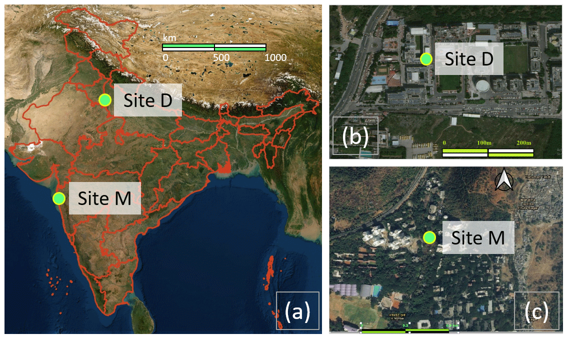
Figure 1A map showing the locations of the deployment sites. Panels (b) and (c) show a local-scale map of the vicinity of the deployment sites – namely site D at MRIIRS, Delhi NCR (b), and site M at MPCB, Mumbai (c), with the sites themselves pointed out using bright green dots. Panel (a) shows the location of the sites on a map of India. Credit for map sources: (a) is taken from the NASA Earth Observatory with the outlines of the Indian states in red taken from QGIS 3.4 Madeira; (b) and (c) are obtained from © Google Maps. The green markers for the sites in all figures were added separately.

Figure 2Panels (a, b) present time series for raw parameters measured using the reference monitors (NO2 and O3 concentrations) as well as those measured using the SATVAM LCAQ sensors (RH, T, no2op1, no2op2, oxop1, oxop2). Panel (a) considers a 48 h period during the June deployment (1–2 July 2019) at site D with signal measurements taken from the sensor DD1 whereas (b) considers a 48 h period during the October deployment (20–21 October 2019) at site M with signal measurements taken from the sensor MM5 (see Sect. 2.3 for conventions used in naming sensors e.g., DD1, MM5). Values for site D are available at 1 min intervals, while those for site M are averaged over 15 min intervals. Thus, the left plot is more granular than the right plot. Site D experiences higher levels of both NO2 and O3 as compared to site M. Panel (c) presents a scatterplot showing variations in RH and T at the two sites across the two deployments. The sites offer substantially diverse weather conditions. Site D exhibits wide variations in RH and T levels during both deployments. Site M exhibits almost uniformly high RH levels during the October deployment which coincided with the retreating monsoons.
2.1 Deployment sites
SATVAM LCAQ sensor deployment and co-location with reference monitors was carried out at two sites. Figure 1 presents the geographical locations of these two sites.
-
Site D. Located within the Delhi (hence site D) National Capital Region (NCR) of India at the Manav Rachna International Institute of Research and Studies (MRIIRS), Sector 43, Faridabad (28.45∘ N, 77.28∘ E; 209 m a.m.s.l. – above mean sea level).
-
Site M. Located within the city of Mumbai (hence site M) at the Maharashtra Pollution Control Board (MPCB) within the university campus of IIT Bombay (19.13∘ N, 72.91∘ E; 50 m a.m.s.l.).
Figure 2 presents a snapshot of raw parameter values presented by the two sites. We refer readers to the supplementary material for additional details about the two deployment sites. Due to increasing economic and industrial activities, a progressive worsening of ambient air pollution is witnessed at both sites. We considered these two sites to cover a broader range of pollutant concentrations and weather patterns, so as to be able to test the reliability of LCAQ networks. It is notable that the two chosen sites present different geographical settings as well as different air pollution levels with site D of particular interest in presenting significantly higher minimum O3 levels than site M, illustrating the influence of the geographical variability over the selected region.
2.2 Instrumentation
LCAQ sensor design. Each SATVAM LCAQ device contains two commodity electrochemical gas sensors (Alphasense OX-B421 and NO2-B42F) for measuring O3 (ppb) and NO2 (ppb) levels, a PM sensor (Plantower PMS7003) for measuring PM2.5 (µg m−3) levels, and a DHT22 sensor for measuring ambient temperature (∘C) and relative humidity RH (%). Figure 3 shows the placement of these components. A notable feature of this device is its focus on frugality and use of the low-power Contiki OS platform and 6LoWPAN for providing wireless-sensor-network connectivity.
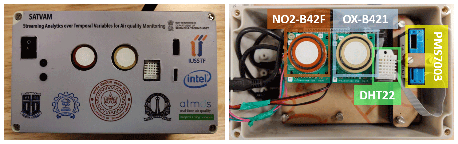
Figure 3Primary components of the SATVAM LCAQ (low-cost air-quality) sensor used in our experiments. The SATVAM device consists of a Plantower PMS7003 PM2.5 sensor, Alphasense OX-B431 and NO2-B43F electrochemical sensors, and a DHT22 RH and temperature sensor. Additional components (not shown here) include instrumentation to enable data collection and transmission.
Detailed information on assembling these different components and the interfacing with an IoT network is described in Simmhan et al. (2019). These sensors form a highly portable IoT software platform to transmit 6LoWPAN packets at 5 min intervals containing five time series data points from individual sensors, namely NO2, O3, PM2.5 (not considered in this study), temperature and RH. Given the large number of devices spread across two cities and seasons in this study, a single border-router edge device was configured at both sites using a Raspberry Pi that acquired data, integrated them and connected to a cloud facility using a Wi-Fi link to the respective campus broadband networks. A Microsoft Azure Standard D4s v3 VM was used to host the cloud service with four cores, 16 GB RAM and 100 GB SSD storage running an Ubuntu 16.04.1 LTS OS. The Pi edge device was designed to ensure that data acquisition continues even in the event of cloud VM failure.
Reference monitors. At both the deployment sites, O3 and NO2 were measured simultaneously with data available at 1 min intervals for site D deployments (both Jun and Oct) and 15 min intervals for site M deployments. O3 and NO2 values were measured at site D using an ultraviolet photometric O3 analyzer (Model 49i O3 analyzer, Thermo Scientific™, USA) and a chemiluminescence oxide of nitrogen (NOx) analyzer (Model 42i NOx analyzer, Thermo Scientific™, USA), respectively. Regular maintenance and multi-point calibration, zero checks, and zero settings of the instruments were carried out following the method described by Gaur et al. (2014). The lowest detectable limits of reference monitors in measuring O3 and NO2 were 0.5 and 0.40 ppb, respectively, and with a precision of ± 0.25 and ± 0.2 ppb, respectively. Similarly, the deployments at site M had Teledyne T200 and T400 reference-grade monitors installed. These also have a UV photometric analyzer to measure O3 levels and use chemiluminescence to measure NO2 concentrations with lowest detectable limits for O3 and NO2 of 0.4 and 0.2 ppb, respectively, and a precision of ± 0.2 and ± 0.1 ppb, respectively. For every deployment, the reference monitors and the AQ sensors were time-synchronized, with the 1 min interval data averaged across 15 min intervals for all site M deployments since the site M reference monitors gave data at 15 min intervals.
2.3 Deployment details
A total of four field co-location deployments, two each at sites D and M, were evaluated to characterize the calibration of the low-cost sensors during two seasons of 2019. The two field deployments at site D were carried out from 27 June–6 August 2019 (7 weeks) and 4–27 October 2019 (3 weeks). The two field deployments at site M, on the other hand, were carried out from 22 June–21 August 2019 (10 weeks) and 4–27 October 2019 (3 weeks). For the sake of convenience, we will refer to both deployments that commenced in the month of June 2019 (October 2019) as June (October) deployments even though the dates of both June deployments do not exactly coincide.

Figure 4A schematic showing the deployment of the six LCAQ sensors across site D and site M during the two deployments. The sensors subjected to the swap-out experiment are presented in bold. Credit for map sources: the outlines of the Indian states in red are taken from QGIS 3.4 Madeira with other highlights (e.g., for oceans) and markers being added separately.
A total of six low-cost SATVAM LCAQ sensors were deployed at these two sites. We assign each of these sensors a unique numerical identifier and a name that describes its deployment pattern. The name of a sensor is of the form XYn where X (Y) indicates the site at which the sensor was deployed during the June (October) deployment and n denotes its unique numerical identifier. Figure 4 outlines the deployment patterns for the six sensors DD1, DM2, DD3, MM5, MD6 and MD7.
Swap-out experiment. As Fig. 4 indicates, three sensors were swapped with the other site across the two deployments. Specifically, for the October deployment, DM2 was shifted from site D to M and MD6 and MD7 were shifted from site M to D.
Sensor malfunction. We actually deployed a total of seven sensors in our experiments. The seventh sensor, named DM4, was supposed to be swapped from site D to site M. However, the onboard RH and temperature sensors for this sensor were non-functional for the entire duration of the June deployment and frequently so for the October deployment as well. For this reason, this sensor was excluded from our study altogether. To avoid confusion, in the rest of the paper (e.g., the abstract, Fig. 4) we report only six sensors, of which three were a part of the swap-out experiment.
All experiments were conducted on a commodity laptop with an Intel Core i7 CPU (2.70 GHz, 8 GB RAM) and running an Ubuntu 18.04.4 LTS operating system. Standard off-the-shelf machine-learning and statistical-analysis packages such as NumPy, sklearn, SciPy and metric-learn were used to implement the calibration algorithms.
Table 1Samples of the raw data collected from the DM2(June) and MM5(October) datasets. The last column indicates whether data from that timestamp were used in the analysis or not. Note that DM2(June) data, coming from site D, have samples at 1 min intervals whereas MM5(October) data, coming from site M, have samples at 15 min intervals. The raw voltage values (no2op1, no2op2, oxop1, oxop2) offered by the LCAQ sensor are always integer values, as indicated in the DM2(June) data. However, for site M deployments, due to averaging, the effective-voltage values used in the dataset may be fractional, as indicated in the MM5(October) data. The symbol × indicates missing values. A bold font indicates invalid values. Times are given in local time.

Raw datasets and features. The six sensors across the June and October deployments gave us a total of 12 datasets. We refer to each dataset by mentioning the sensor name and the deployment. For example, the dataset DM2(Oct) contains data from the October deployment at site M of the sensor DM2. Each dataset is represented as a collection of eight time series for which each timestamp is represented as an 8-tuple (O3, NO2, RH, T, no2op1, no2op2, oxop1, oxop2) giving us the reference values for O3 and NO2 (in ppb), relative humidity RH (in %) and temperature T (in ∘C) values, and voltage readings (in mV) from the two electrodes present in each of the two gas sensors, respectively. These readings represent working (no2op1 and oxop1) and auxiliary (no2op2 and oxop2) electrode potentials for these sensors. We note that RH and T values in all our experiments were obtained from DHT22 sensors in the LCAQ sensors and not from the reference monitors. This was done to ensure that the calibration models, once trained, could perform predictions using data available from the LCAQ sensor alone and did not rely on data from a reference monitor. For site D, both the LCAQ sensor and the reference monitor data were available at 1 min intervals. However for site M, since reference monitor data were only available at 15 min intervals, LCAQ sensor data were averaged over 15 min intervals.
Data cleanup. Timestamps from the LCAQ sensors were aligned to those from the reference monitors. For several timestamps, we found that either the sensor or reference monitors presented at least one missing or spurious value (see Table 1 for examples). Spurious values included the following cases: (a) a reference value for O3 or NO2 of >200 ppb or <0 ppb (the reference monitors sometimes offered negative readings when powering up and under anomalous operating conditions, e.g., condensation at the inlet), (b) a sensor temperature reading of >50 ∘C or <1 ∘C, (c) a sensor RH level of >100 % or <1 %, and (d) a sensor voltage reading (any of no2op1, no2op2, oxop1, oxop2) of >400 mV or <1 mV. These errors are possibly due to electronic noise in the devices. All timestamps with even one spurious or missing value were considered invalid and removed. Across all 12 datasets, an average of 52 % of the timestamps were removed as a result. However, since site D (site M) offered timestamps at 1 min (15 min) intervals i.e., 60 (4) timestamps every hour, at least one valid timestamp (frequently several) was still found every hour in most cases. Thus, the valid timestamps could still accurately track diurnal changes in AQ parameters. The datasets from June (October) deployments at site D offered an average of 33 753 (9548) valid timestamps. The datasets from June (October) deployments in site M offered an average of 2462 (1062) valid timestamps. As expected, site D which had data at 1 min intervals offered more timestamps than site M which had data at 15 min intervals. For both sites, more data are available for the June deployment (that lasted longer) than the October deployment.
3.1 Data augmentation and derived dataset creation
For each of the 12 datasets, apart from the six data features provided by the LCAQ sensors, we included two augmented features, calculated as follows: , and . We found that having these augmented features, although they are simple linear combinations of raw features, offered our calibration models a predictive advantage. The augmented datasets created this way represented each timestamp as a vector of eight feature values (RH, T, no2op1, no2op2, oxop1, oxop2, no2diff, oxdiff), apart from the reference values of O3 and NO2.
3.1.1 Train–test splits
Each of the 12 datasets was split in a 70:30 ratio to obtain a train–test split. For each dataset, 10 such splits were independently generated. All calibration algorithms were given the same train–test splits. For algorithms that required hyperparameter tuning, a randomly chosen set of 30 % of the training data points in each split was used as a held-out validation set. All features were normalized to improve the conditioning of the calibration problems. This was done by calculating the mean and standard deviation for each of the eight features on the training portion of a split and then mean centering and dividing by the standard deviation all timestamps in both the training and the testing portion of that split. An exception was made for the Alphasense calibration models, which required raw voltage values. However, reference values were not normalized.
3.2 Derived datasets
In order to study the effect of data frequency (how frequently do we record data, e.g., 1 min, 15 min?), data volume (total number of timestamps used for training) and data diversity (data collected across seasons or sites) on the calibration performance, we created several derived datasets as well. All these datasets contained the augmented features.
-
Temporally averaged datasets. We took the two datasets DD1(Jun) and DM2(Jun) and created four datasets out of each of them by averaging the sensor and reference monitor values at 5, 15, 30 and 60 min intervals. These datasets were named by affixing the averaging interval size to the dataset name. For example, DD1(Jun)-AVG5 was created out of DD1(Jun) by performing 5 min averaging and DM2(Jun)-AVG30 was created out of DM2(Jun) using 30 min averaging.
-
Sub-sampled datasets. To study the effect of having fewer training data on calibration performance, we created sub-sampled versions of both these datasets by sampling a random set of 2500 timestamps from the training portion of the DD1(June) and DM2(June) datasets to get the datasets named DD1(June)-SMALL and DM2(June)-SMALL.
-
Aggregated datasets. Next, we created new datasets by pooling data for a sensor across the two deployments. This was done to the data from the sensors DD1, MM5, DM2 and MD6. For example, if we consider the sensor DD1, then the datasets DD1(June) and DD1(October) were combined to create the dataset DD1(June–October).
Investigating impact of diversity in data. The aggregated datasets are meant to help us study how calibration algorithms perform under seasonally and spatially diverse data. For example, the datasets DD1(June–October) and MM5(June–October) include data that are seasonally diverse but not spatially diverse (since these two sensors were located at the same site for both deployments). On the other hand, the datasets DM2(June–October) and MD6(June–October) include data that are diverse both seasonally and spatially (since these two sensors were a part of the swap-out experiment). At this point, it is natural to wonder about studying the effect of spatial diversity alone (without seasonal effects). This can be done by aggregating data from two distinct sensors since no sensor was located at both sites during a deployment. However, this turns out to be challenging since the onboard sensors in the LCAQ devices, e.g., RH and T sensors, do not present good agreement across devices, and some form of cross-device calibration is needed. This is an encouraging direction for future work but not considered in this study.
3.2.1 Performance evaluation
The performance of calibration algorithms was assessed using standard error metrics and statistical hypothesis testing.
Error metrics. Calibration performance was measured using four popular metrics: mean absolute error (MAE), mean absolute percentage error (MAPE), root mean squared error (RMSE), and the coefficient of determination (R2) (please see the supplementary material for detailed expressions of these metrics).
Statistical hypothesis tests. In order to compare the performance of different calibration algorithms on a given dataset (to find out the best-performing algorithm) or to compare the performance of the same algorithm on different datasets (to find out the effect of data characteristics on calibration performance), we performed paired and unpaired two-sample tests, respectively. Our null hypothesis in all such tests proposed that the absolute errors offered in the two cases considered are distributed identically. The test was applied, and if the null hypothesis was rejected with sufficient confidence (an α value of 0.05 was used as the standard to reject the null hypotheses), then a winner was simultaneously identified. Although Student's t test is more popular, it assumes that the underlying distributions are normal, and an application of the Shapiro–Wilk test (Shapiro and Wilk, 1965) to our absolute error values rejected the normal hypothesis with high confidence. Thus, we chose the non-parametric Wilcoxon signed-rank test (Wilcoxon, 1945) when comparing two algorithms on the same dataset and its unpaired variant, the Mann–Whitney U test (Mann and Whitney, 1947) for comparing the same algorithm on two different datasets. These tests do not make any assumption about the underlying distribution of the errors and are well-suited for our data.
Our study considered a large number of parametric and non-parametric calibration techniques as baseline algorithms. Table 2 provides a glossary of all the algorithms including their acronyms and brief descriptions. Detailed descriptions of all these algorithms are provided in the supplementary material. Among parametric algorithms, we considered the Alphasense models (AS1–AS4) supplied by the manufacturers of the gas sensors and linear models based on least squares (LS and LS(MIN)) and sparse recovery (LASSO). Among non-parametric algorithms, we considered the regression tree (RT) method, kernel-ridge regression (KRR), the Nystroem method for accelerating KRR, the Nadaraya–Watson (NW) estimator and various local algorithms based on the k nearest-neighbors principle (KNN, KNN-D). In this section we give a self-contained description of our proposed algorithms KNN(ML) and KNN-D(ML).
Table 2Glossary of baseline and proposed calibration algorithms used in our study with their acronyms and brief descriptions. The KNN(ML) and KNN-D(ML) algorithms are proposed in this paper. Please see the Supplement for details.

∗ Proposed in this paper.
Notation. For every timestamp t, the vector xt∈ℝ8 denotes the 8-dimensional vector of signals recorded by the LCAQ sensors for that timestamp (namely, RH, T, no2op1, no2op2, oxop1, oxop2, no2diff, oxdiff), while the vector yt∈ℝ2 will denote the 2-tuple of the reference values of O3 and NO2 for that time step. However, this notation is unnecessarily cumbersome since we will build separate calibration models for O3 and NO2. Thus, to simplify the notation, we will instead use yt∈ℝ to denote the reference value of the gas being considered (either O3 or NO2). The goal of calibration will then be to learn a real-valued function such that f(xt)≈yt for all timestamps t (the exact error being measured using metrics such as MAE or MAPE). Thus, two functions will be learned, say and , to calibrate for NO2 and O3 concentrations, respectively. Since our calibration algorithms use statistical estimation or machine learning algorithms, we will let N (n) denote the number of training (testing) points for a given dataset and split thereof. Thus, will denote the training set for a given dataset and split with xt∈ℝ8 and yt∈ℝ.
4.1 Proposed method – distance-weighed KNN with a learned metric
Our proposed algorithm is a local, non-parametric algorithm that uses a learned metric. Below we describe the design of this method and reasons behind these design choices.
Table 3Results of the pairwise Wilcoxon signed-rank tests across all model types. We refer the reader to Sect. 5.1.1 for a discussion on how to interpret this table. KNN-D(ML) beats every other algorithm comprehensively and is scarcely ever beaten (with the exception of NW(ML), which KNN-D(ML) still beats 58 % of the time for NO2 and 62 % of the time for O3). The overall ranking of the algorithms is indicated to be KNN-D(ML) > NW(ML) > KRR > RT > LS.
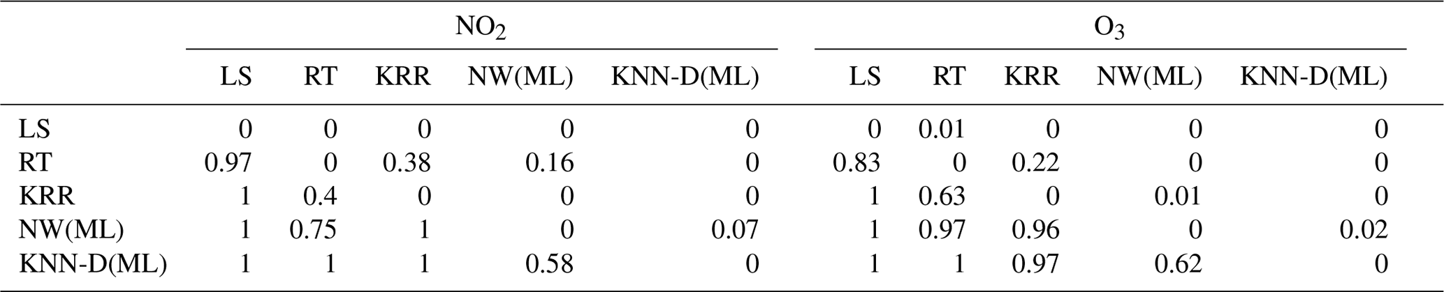
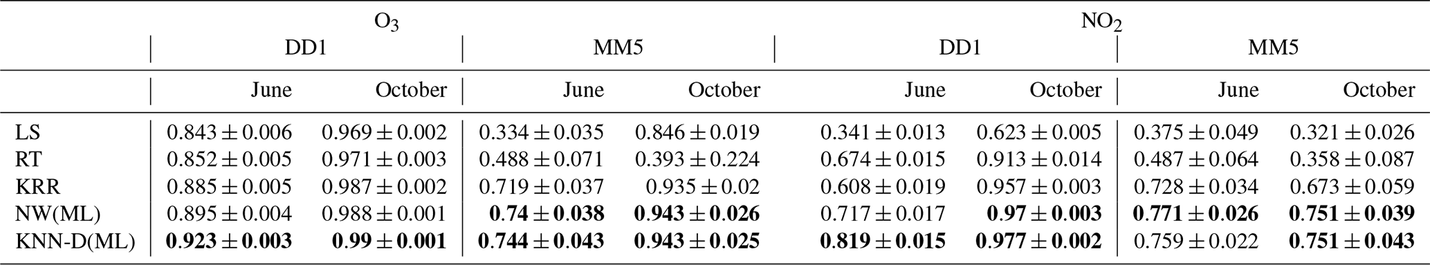
Table 4A comparison of algorithms across families on the DD1 and MM5 datasets across seasons with respect to the R2 metric. All values are averaged across 10 splits. Bold values indicate the best-performing algorithm in terms of mean statistics.
Non-parametric estimators for calibration. The simplest example of a non-parametric estimator is the KNN (k nearest-neighbors) algorithm that predicts, for a test point, the average reference value in the k most similar training points also known as “neighbors”. Other examples of non-parametric algorithms include kernel ridge regression (KRR) and the Nadaraya–Watson (NW) estimator (please see the supplementary material for details). Non-parametric estimators are well-studied and known to be asymptotically universal which guarantees their ability to accurately model complex patterns which motivated our choice. These models can also be brittle (Hagan et al., 2019) when used in unseen operating conditions, but Sect. 5.2 shows that our proposed algorithm performs comparably to parametric algorithms when generalizing to unseen conditions but offers many more improvements when given additional data.
Metric learning for KNN calibration. As mentioned above, the KNN algorithm uses neighboring points to perform prediction. A notion of distance, specifically a metric, is required to identify neighbors. The default and most common choice for a metric is the Euclidean distance which gives equal importance to all eight dimensions when calculating distances between two points, say . However, our experiments in Sect. 5 will show that certain features, e.g., RH and T, seem to have a significant influence on calibration performance. Thus, it is unclear how much emphasis RH and T should receive, as compared to other features such as voltage values, e.g., oxop1, while calculating distances between two points. The technique of metric learning (Weinberger and Saul, 2009) offers a solution in this respect by learning a customized Mahalanobis metric that can be used instead of the generic Euclidean metric. A Mahalanobis metric is characterized by a positive semi-definite matrix and calculates the distance between any two points as follows:
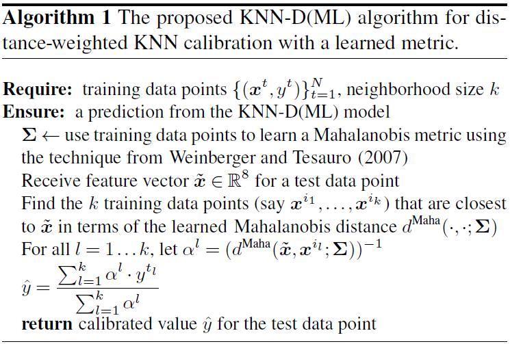
Note that the Mahalanobis metric recovers the Euclidean metric if we choose Σ=I8, i.e., the identity matrix. Now, whereas metric learning for KNN is popular for classification problems, it is uncommon for calibration and regression problems. This is due to regression problems lacking a small number of “classes”. To overcome this problem, we note that other non-parametric calibration algorithms such as NW and KRR also utilize a metric indirectly (please see the supplementary material) and there exist techniques to learn a Mahalanobis metric to be used along with these algorithms (Weinberger and Tesauro, 2007). This allows us to adopt a two-stage algorithm that first learns a Mahalanobis metric well-suited for use with the NW algorithm and then uses it to perform KNN-style calibration. Algorithm 1 describes the resulting KNN-D(ML) algorithm.
The goals of using low-cost AQ monitoring sensors vary widely. This section critically assesses a wide variety of calibration models. First we look at the performance of the algorithms on individual datasets, i.e., when looking at data within a site and within a season. Next, we look at derived datasets (see Sect. 3.2) which consider the effect of data volume, data averaging and data diversity on calibration performance.
5.1 Effect of model on calibration performance
We compare the performance of calibration algorithms introduced in Sect. 4. Given the vast number of algorithms, we executed a tournament where algorithms were divided into small families, decided the winner within each family and then compared winners across families. The detailed per-family comparisons are available in the supplementary material and summarized here. The Wilcoxon paired two-sample test (see Sect. 3.2.1) was used to compare two calibration algorithms on the same dataset. However, for visual inspection, we also provide violin plots of the absolute errors offered by the algorithms. We refer the reader to the supplementary material for pointers on how to interpret violin plots.
5.1.1 Interpreting the two-sample tests
We refer the reader to Table 2 for a glossary of algorithm names and abbreviations. As mentioned earlier, we used the paired Wilcoxon signed-rank test to compare two algorithms on the same dataset. Given that there are 12 datasets and 10 splits for each dataset, for ease of comprehension, we provide globally averaged statistics of wins scored by an algorithm over another. For example, say we wish to compare RT and KRR as done in Table 3, we perform the test for each individual dataset and split. For each test, we get a win for RT (in which case RT gets a +1 score and KRR gets 0) or a win for KRR (in which case KRR gets a +1 score and RT gets 0) or else the null hypothesis is not refuted (in which case both get 0). The average of these scores is then shown. For example, in Table 3, row 3–column 7 (excluding column and row headers) records a value of 0.63 implying that in 63 % of these tests, KRR won over RT in the case of O3 calibration, whereas row 2–column 8 records a value of 0.22, implying that in 22 % of the tests, RT won over KRR. On balance () i.e., 15 % of the tests, neither algorithm could be declared a winner.
5.1.2 Intra-family comparison of calibration models
We divided the calibration algorithms (see Table 2 for a glossary) into four families: (1) the Alphasense family (AS1, AS2, AS3, AS4), (2) linear parametric models (LS, LS(MIN) and LASSO), (3) kernel regression models (KRR, NYS), and (4) KNN-style algorithms (KNN, KNN-D, NW(ML), KNN(ML), KNN-D(ML)). We included the Nadaraya–Watson (NW) algorithm in the fourth family since it was used along with metric learning, as well as because as explained in the supplementary material, the NW algorithm behaves like a “smoothed” version of the KNN algorithm. The winners within these families are described below.
-
Alphasense. All four Alphasense algorithms exhibit extremely poor performance across all metrics on all datasets, offering extremely high MAE and low R2 values. This is corroborated by previous studies (Lewis and Edwards, 2016; Jiao et al., 2016; Simmhan et al., 2019).
-
Linear parametric. Among the linear parametric algorithms, LS was found to offer the best performance.
-
Kernel regression. The Nystroem method (NYS) was confirmed to be an accurate but accelerated approximation for KRR with the acceleration being higher for larger datasets.
-
KNN and metric-learning models. Among the KNN family of algorithms, KNN-D(ML), i.e., distance-weighted KNN with a learned metric, was found to offer the best accuracies across all datasets and splits.
5.1.3 Global comparison of comparison models
We took the best algorithms from all the families (except Alphasense models that gave extremely poor performance) and regression trees (RT) and performed a head-to-head comparison to assess the winner. The two-sample tests (Table 3) as well as violin plots (Fig. 5) indicate that the KNN-D(ML) algorithm continues to emerge as the overall winner. Table 4 additionally establishes that KNN-D(ML) can be up to 4–20 percentage points better than classical non-parametric algorithms such as KRR in terms of the R2 coefficient. The improvement is much more prominent for NO2 calibration which seems to be more challenging as compared to O3 calibration. Figure 6 presents cases where the KNN-D(ML) models offer excellent agreement with the reference monitors across significant spans of time.

Figure 5The violin plots on the left (a) show the distribution of absolute errors incurred by various models on the DD1(October) (MM5(June)) datasets. KNN-D(ML) offers visibly superior performance as compared to other algorithms such as LS and RT.
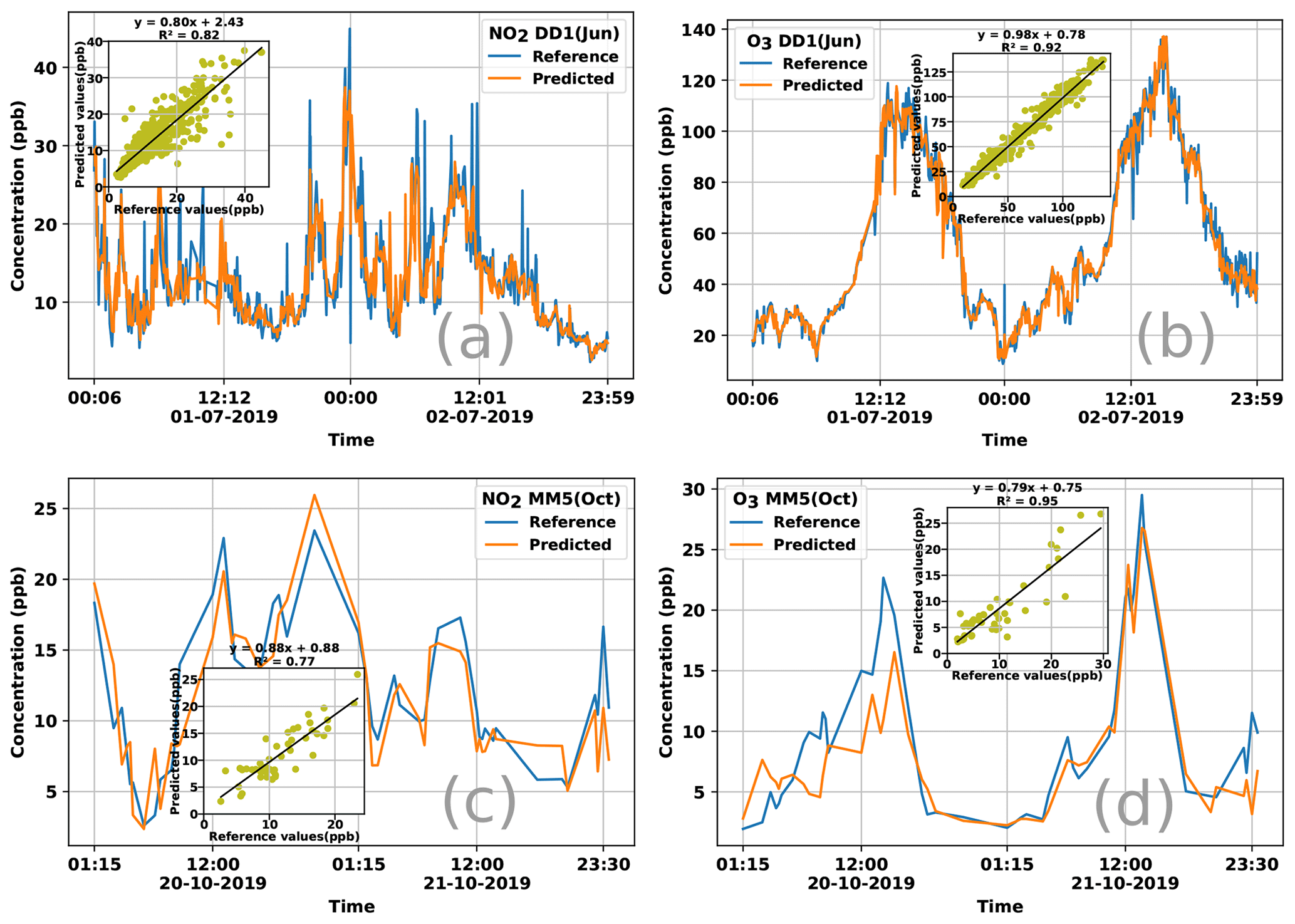
Figure 6Time series plotting reference values and those predicted by the KNN-D(ML) algorithm for NO2 and O3 concentration for 48 h durations using data from the DD1 and MM5 sensors. The legend of each plot notes the gas for which calibration is being reported and the deployment season, as well as the sensor from which data were used to perform the calibration. Each plot also contains a scatterplot as an inset showing the correlation between the reference and predicted values of the concentrations. For both deployments and both gases, KNN-D(ML) can be seen to offer excellent calibration and agreement with the FRM-grade monitor.
Analyzing high-error patterns. Having analyzed the calibration performance of various algorithms including KNN-D(ML), it is interesting to note under what conditions these algorithms incur high error. Non-parametric algorithms such as RT and KNN-D(ML) are expected to do well in the presence of good quantities of diverse data. Figure 7 confirms this by classifying timestamps into various bins according to weather conditions. KNN-D(ML) and RT give high average error mostly in those bins where there were fewer training points. Figure 7 also confirms a positive correlation between high concentrations and higher error although this effect is more pronounced for LS than for KNN-D(ML).
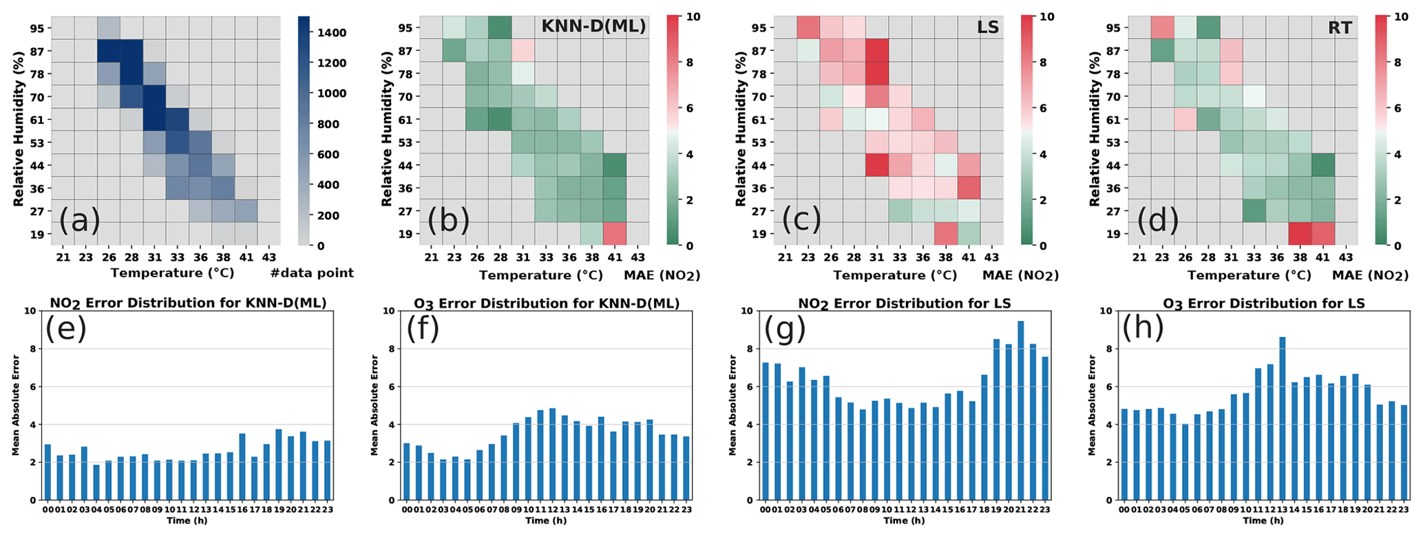
Figure 7Analyzing error distributions of LS, KNN-D(ML) and RT. Panel (a) shows the number of training data points in various weather condition bins. Panels (b, c, d) show the MAE for NO2 calibration offered by the algorithms in those same bins. Non-parametric algorithms such as KNN-D(ML) and RT offer poor performance (high MAE) mostly in bins that had fewer training data. No such pattern is observable for LS. Panels (e, f, g, h) show the diurnal variation in MAE for KNN-D(ML) and LS at various times of day. O3 errors exhibit a diurnal trend of being higher (more so for LS than for KNN-D(ML)) during daylight hours when O3 levels are high. No such trend is visible for NO2.
5.2 Effect of data preparation on calibration performance
We critically assessed the robustness of these calibration models and identified the effect of other factors, such as temporal averaging of raw data, total number of data available for training and diversity in training data. We note that some of these studies were made possible only because the swap-out experiment enabled us to have access to sensors that did not change their deployment sites, as well as to those that did change their deployment site.
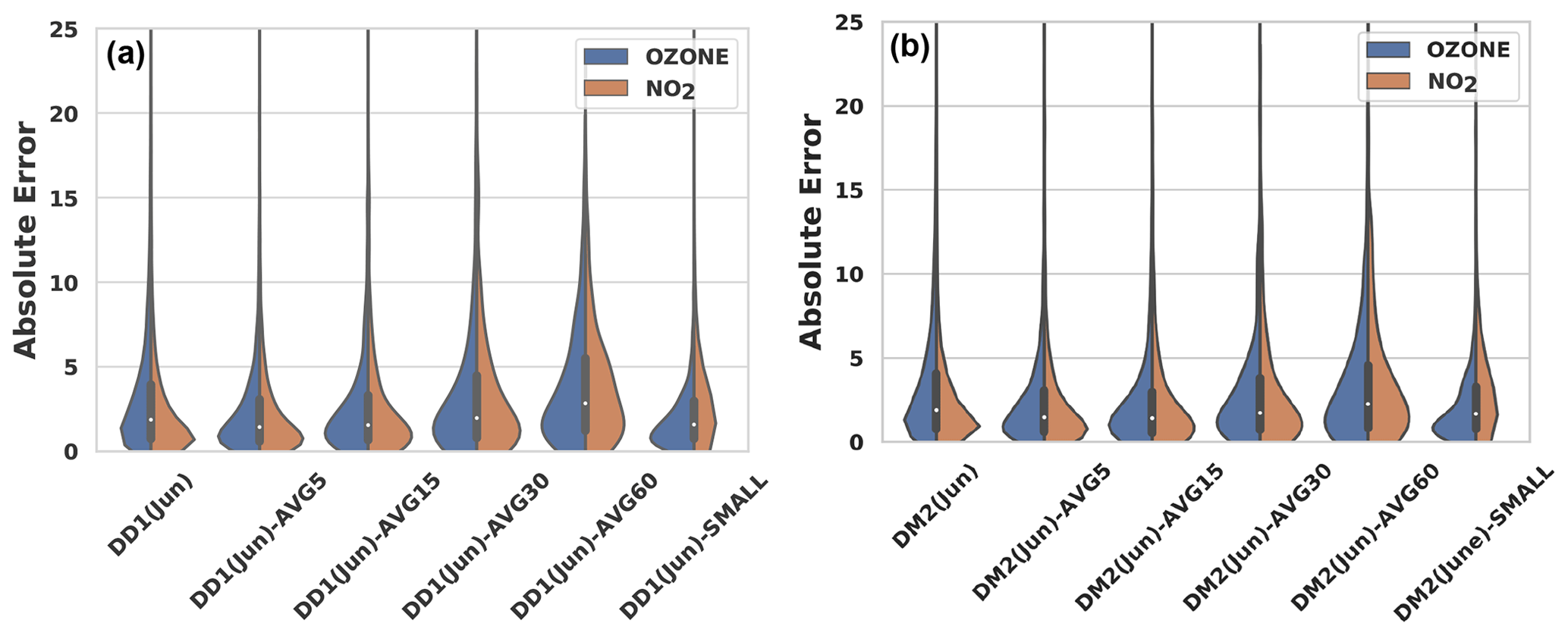
Figure 8Effect of temporal data averaging and lack of data on the calibration performance of the KNN-D(ML) algorithm on temporally averaged and sub-sampled versions of the DD1(June) and DM2(June) datasets. Notice the visible deterioration in the performance of the algorithm when aggressive temporal averaging, e.g., across 30 min windows, is performed. NO2 calibration performance seems to be impacted more adversely than O3 calibration by lack of enough training data or aggressive averaging.
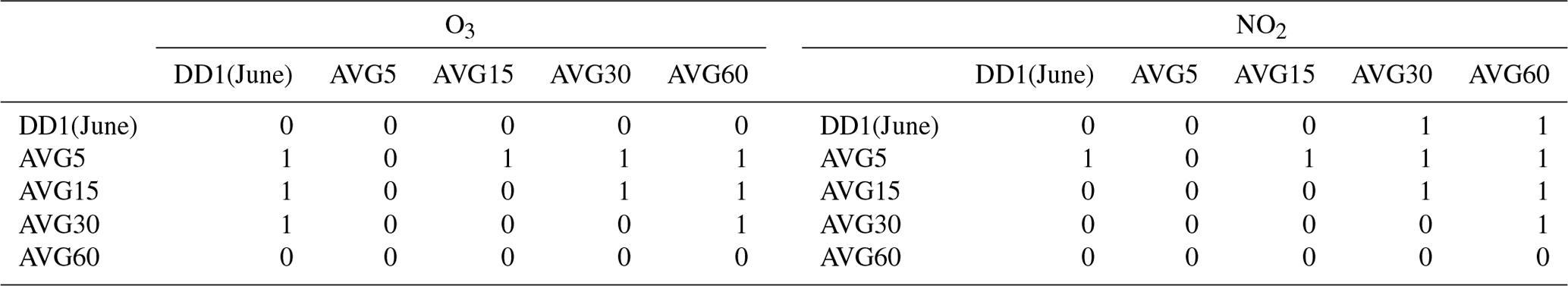
Table 5Results of the pairwise Mann–Whitney U tests on the performance of KNN-D(ML) across temporally averaged versions of the DD1 dataset. We refer the reader to Sect. 5.1.1 for a discussion on how to interpret this table. The dataset names are abbreviated, e.g., DD1(June)-AVG5 is referred to as simply AVG5. Results are reported over a single split. AVG5 wins over any other level of averaging and clarifies that mild temporal averaging (e.g., over 5 min windows) boosts calibration performance, whereas aggressive averaging, e.g., 60 min averaging in AVG60, degrades performance.
5.2.1 Some observations on original datasets
The performance of KNN-D(ML) on the original datasets itself gives us indications of how various data preparation methods can affect calibration performance. Table 4 shows us that in most cases, the calibration performance is better (with higher R2) for O3 than for NO2. This is another indication that NO2 calibration is more challenging than O3 calibration. Moreover, for both gases and in both seasons, we see site D offering a better performance than site M. This difference is more prominent for NO2 than for O3. This indicates that paucity of data and temporal averaging may be affecting calibration performance negatively, as well as that O3 calibration might be less sensitive to these factors than NO2 calibration.
5.2.2 Effect of temporal data averaging
Recall that data from sensors deployed at site M had to be averaged over 15 min intervals to align them with the reference monitor timestamps. To see what effect such averaging has on calibration performance, we use the temporally averaged datasets (see Sect. 3.1). Figure 8 presents the results of applying the KNN-D(ML) algorithm on data that are not averaged at all (i.e., 1 min interval timestamps), as well as data that are averaged at 5, 15, 30 and 60 min intervals. The performance for 30 and 60 min averaged datasets is visibly inferior than for the non-averaged dataset as indicated by the violin plots. This leads us to conclude that excessive averaging can erode the diversity of data and hamper effective calibration. To distinguish among the other temporally averaged datasets for which visual inspection is not satisfactory, we also performed the unpaired Mann–Whitney U test, the results for which are shown in Table 5. The results are striking in that they reveal that moderate averaging, for example at 5 min intervals, seems to benefit calibration performance. However, this benefit is quickly lost if the averaging window is increased much further, at which point performance almost always suffers. NO2 calibration performance seems to be impacted more adversely than O3 calibration by aggressive averaging.
5.2.3 Effect of data paucity
Since temporal averaging decreases the number of data as a side-effect, in order to tease these two effects (of the temporal averaging and of the paucity of data) apart, we also considered the sub-sampled versions of these datasets (see Sect. 3.1). Figure 8 also shows that reducing the number of training data has an appreciable negative impact on calibration performance. NO2 calibration performance seems to be impacted more adversely than O3 calibration by lack of enough training data.
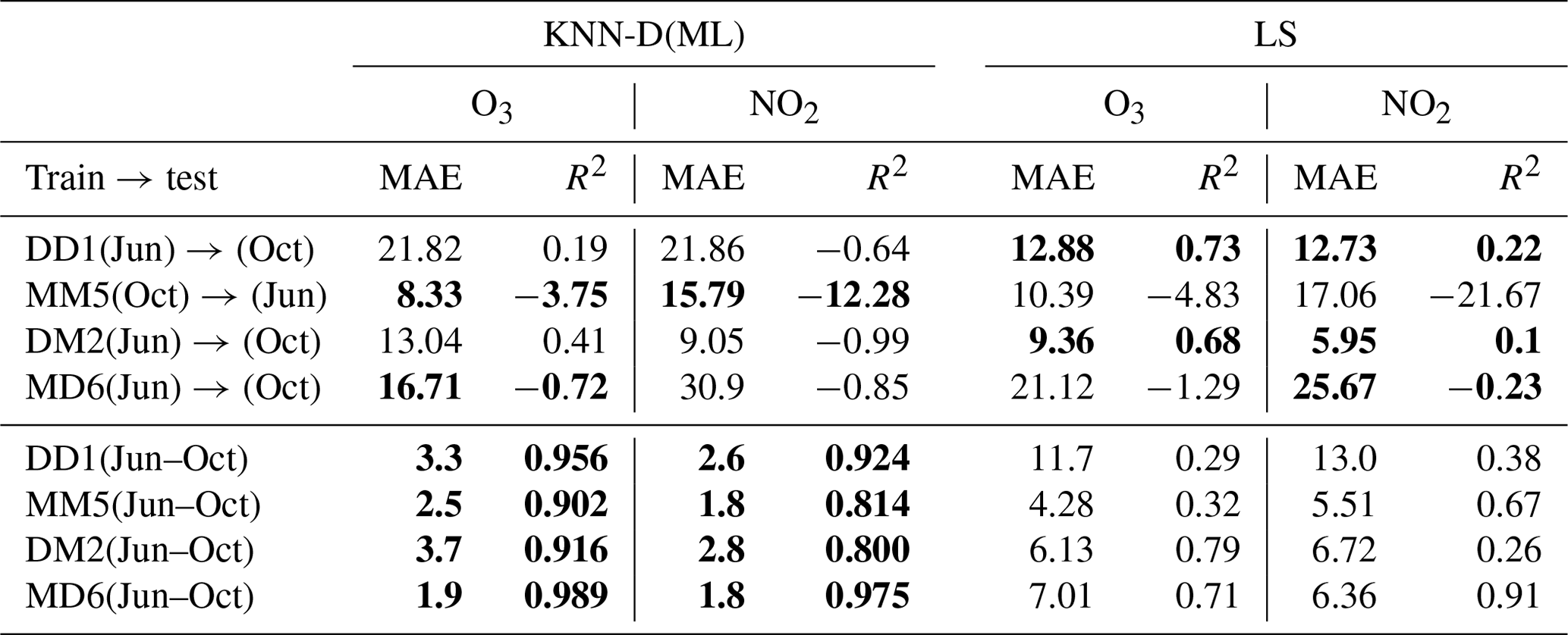
Table 6A demonstration of the impact of data diversity and data volume on calibration performance. All values are averaged across 10 splits. The results for LS diverged for some of the datasets for a few splits, and those splits were removed while averaging to give LS an added advantage. Bold values indicate the better-performing algorithm. The first two rows present the performance of the KNN-D(ML) and LS calibration models when tested on data for a different season (deployment) but in the same site. This was done for the DD1 and MM5 sensors that did not participate in the swap-out experiment. The next two rows present the same but for sensors DM2 and MD6 that did participate in the swap-out experiment, and thus, their performance is being tested for not only a different season but also a different site. The next four rows present the dramatic improvement in calibration performance once datasets are aggregated for these four sensors. NO2 calibration is affected worse by these variations (average R2 in first four rows being −3.69) than O3 calibration (average R2 in first four rows being −0.97).
5.2.4 The swap-out experiment – effect of data diversity
Table 6 describes an experiment wherein we took the KNN-D(ML) model trained on one dataset and used it to make predictions on another dataset. To avoid bringing in too many variables such as cross-device calibration (see Sect. 3.2), this was done only in cases where both datasets belonged to the same sensor but for different deployments. Without exception, such “transfers” led to a drop in performance. We confirmed that this was true for not just non-parametric methods such as KNN-D(ML) but also parametric models like LS. This is to be expected since the sites D and M experience largely non-overlapping ranges of RH and T across the two deployments (see Fig. 2c for a plot of RH and T values experienced at both sites in both deployments). Thus, it is not surprising that the models performed poorly when faced with unseen RH and T ranges. To verify that this is indeed the case, we ran the KNN-D(ML) algorithm on the aggregated datasets (see Sect. 3.1) which combine training sets from the two deployments of these sensors. Table 6 confirms that once trained on these more diverse datasets, the algorithms resume offering good calibration performance on the entire (broadened) range of RH and T values. However, KNN-D(ML) is more superior at exploiting the additional diversity in data than LS. We note that parametric models are expected to generalize better than non-parametric models for unseen conditions, and indeed we observe this in some cases in Table 6 where, for DD1 and DM2 datasets, LS generalized better than KNN-D(ML). However, we also observe some cases such as MM5 and MD6 where KNN-D(ML) generalizes comparably to or better than LS.
In this study we presented results of field deployments of LCAQ sensors across two seasons and two sites having diverse geographical, meteorological and air pollution parameters. A unique feature of our deployment was the swap-out experiment wherein three of the six sensors were transported across sites in the two deployments. To perform highly accurate calibration of these sensors, we experimented with a wide variety of standard algorithms but found a novel method based on metric learning to offer the strongest results. A few key takeaways from our statistical analyses are as follows:
-
Incorporating ambient RH and T, as well as the augmented features oxdiff and noxdiff (see Sect. 3), into the calibration model improves calibration performance.
-
Non-parametric methods such as KNN offer the best performance but stand to gain significantly through the use of metric-learning techniques, which automatically learn the relative importance of each feature, as well as hyper-local variations such as distance-weighted KNN. The significant improvements offered by non-parametric methods indicate that these calibration tasks operate in high-variability conditions where local methods offer the best chance of capturing subtle trends.
-
Performing smoothing over raw time series data obtained from the sensors may help improve calibration performance but only if done over short windows. Very aggressive smoothing done over long windows is detrimental to performance.
-
Calibration models are data-hungry as well as diversity-hungry. This is especially true of local methods, for instance KNN variants. Using these techniques limits the number of data or diversity of data in terms of RH, T or concentration levels, which may result in calibration models that generalize poorly.
-
Although all calibration models see a decline in performance when tested in unseen operating conditions, calibration models for O3 seem to be less sensitive than those for NO2 calibration.
Our results offer encouraging options for using LCAQ sensors to complement CAAQMSs in creating dense and portable monitoring networks. Avenues for future work include the study of long-term stability of electrochemical sensors, characterizing drift or deterioration patterns in these sensors and correcting for the same, and the rapid calibration of these sensors that requires minimal co-location with a reference monitor.
The code used in this study is available at the following repository: https://github.com/purushottamkar/aqi-satvam (last access: 5 November 2020; Nagal and Kar, 2020).
The supplement related to this article is available online at: https://doi.org/10.5194/amt-14-37-2021-supplement.
RaS and BM performed measurements. RaS, AN, KKD, HU and PK processed and analyzed the data. RaS, AN and PK wrote the paper. AN and PK developed the KNN-D(ML) calibration algorithm described in Sect. 4 and conducted the data analysis experiments reported in Sect. 5. SM, SN and YS designed and set up the IoT cyber-infrastructure required for data acquisition from the edge to the cloud. BM, RoS and RZ designed the SATVAM LCAQ device and did hardware assembly and fabrication. VMM provided reference-grade data from site M used in this paper. SNT supervised the project, designed and conceptualized the research, provided resources, acquired funding, and helped in writing and revising the paper.
Author Ronak Sutaria is the CEO of Respirer Living Sciences Pvt. Ltd. which builds and deploys low-cost-sensor-based air quality monitors with the trade name “Atmos – Realtime Air Quality”. Ronak Sutaria's involvement was primarily in the development of the air quality sensor monitors and the big-data-enabled application programming interfaces used to access the temporal data but not in the data analysis. Author Brijesh Mishra, subsequent to the work presented in this paper, has joined the Respirer Living Sciences team. The authors declare that they have no other competing interests.
This research has been supported under the Research Initiative for Real Time River Water and Air Quality Monitoring program funded by the Department of Science and Technology, government of India, and Intel® and administered by the Indo-United States Science and Technology Forum (IUSSTF).
This research has been supported by the Indo-United States Science and Technology Forum (IUSSTF) (grant no. IUSSTF/WAQM-Air Quality Project-IIT Kanpur/2017).
This paper was edited by Pierre Herckes and reviewed by three anonymous referees.
Akasiadis, C., Pitsilis, V., and Spyropoulos, C. D.: A Multi-Protocol IoT Platform Based on Open-Source Frameworks, Sensors, 19, 4217, 2019. a
Apte, J. S., Messier, K. P., Gani, S., Brauer, M., Kirchstetter, T. W., Lunden, M. M., Marshall, J. D., Portier, C. J., Vermeulen, R. C., and Hamburg, S. P.: High-Resolution Air Pollution Mapping with Google Street View Cars: Exploiting Big Data, Environ. Sci. Technol., 51, 6999–7008, 2017. a
Arroyo, P., Herrero, J. L., Suárez, J. I., and Lozano, J.: Wireless Sensor Network Combined with Cloud Computing for Air Quality Monitoring, Sensors, 19, 691, 2019. a
Baron, R. and Saffell, J.: Amperometric Gas Sensors as a Low Cost Emerging Technology Platform for Air Quality Monitoring Applications: A Review, ACS Sensors, 2, 1553–1566, 2017. a, b
Castell, N., Dauge, F. R., Schneider, P., Vogt, M., Lerner, U., Fishbain, B., Broday, D., and Bartonova, A.: Can commercial low-cost sensor platforms contribute to air quality monitoring and exposure estimates?, Environ. Int., 99, 293–302, 2017. a
Chowdhury, S., Dey, S., and Smith, K. R.: Ambient PM2.5 exposure and expected premature mortality to 2100 in India under climate change scenarios, Nat. Commun., 9, 1–10, 2018. a
Commodore, A., Wilson, S., Muhammad, O., Svendsen, E., and Pearce, J.: Community-based participatory research for the study of air pollution: a review of motivations, approaches, and outcomes, Environ. Monit. Assess., 189, 378, 2017. a
Cross, E. S., Williams, L. R., Lewis, D. K., Magoon, G. R., Onasch, T. B., Kaminsky, M. L., Worsnop, D. R., and Jayne, J. T.: Use of electrochemical sensors for measurement of air pollution: correcting interference response and validating measurements, Atmos. Meas. Tech., 10, 3575–3588, https://doi.org/10.5194/amt-10-3575-2017, 2017. a
De Vito, S., Esposito, E., Salvato, M., Popoola, O., Formisano, F., Jones, R., and Di Francia, G.: Calibrating chemical multisensory devices for real world applications: An in-depth comparison of quantitative machine learning approaches, Sensor. Actuat. B-Chem., 255, 1191–1210, 2018. a, b
Esposito, E., De Vito, S., Salvato, M., Bright, V., Jones, R., and Popoola, O.: Dynamic neural network architectures for on field stochastic calibration of indicative low cost air quality sensing systems, Sensor. Actuat. B-Chem., 231, 701–713, 2016. a
Fung, P. L.: Calibration of Atmospheric Measurements in Low-cost Sensors, Data Science for Natural Sciences (DSNS'19) Seminar, Department of Computer Science, University of Helsinki, Finland, available at: http://www.edahelsinki.fi/dsns2019/a/dsns2019_fung.pdf, (last access: 16 December 2020), 2019. a
Gabrys, J., Pritchard, H., and Barratt, B.: Just good enough data: Figuring data citizenships through air pollution sensing and data stories, Big Data Soc., 3, 1–14, 2016. a
Garaga, R., Sahu, S. K., and Kota, S. H.: A Review of Air Quality Modeling Studies in India: Local and Regional Scale, Curr. Pollut. Rep., 4, 59–73, 2018. a
Gaur, A., Tripathi, S., Kanawade, V., Tare, V., and Shukla, S.: Four-year measurements of trace gases (SO2, NOx, CO, and O3) at an urban location, Kanpur, in Northern India, J. Atmos. Chem., 71, 283–301, 2014. a
Gillooly, S. E., Zhou, Y., Vallarino, J., Chu, M. T., Michanowicz, D. R., Levy, J. I., and Adamkiewicz, G.: Development of an in-home, real-time air pollutant sensor platform and implications for community use, Environ. Pollut., 244, 440–450, 2019. a
Hagan, D. H., Gani, S., Bhandari, S., Patel, K., Habib, G., Apte, J. S., Hildebrandt Ruiz, L., and Kroll, J. H.: Inferring Aerosol Sources from Low-Cost Air Quality Sensor Measurements: A Case Study in Delhi, India, Environ. Sci. Technol. Lett., 6, 467–472, 2019. a, b, c, d, e
Hitchman, M., Cade, N., Kim Gibbs, T., and Hedley, N. J. M.: Study of the factors affecting mass transport in electrochemical gas sensors, Analyst, 122, 1411–1418, 1997. a
Jiao, W., Hagler, G., Williams, R., Sharpe, R., Brown, R., Garver, D., Judge, R., Caudill, M., Rickard, J., Davis, M., Weinstock, L., Zimmer-Dauphinee, S., and Buckley, K.: Community Air Sensor Network (CAIRSENSE) project: evaluation of low-cost sensor performance in a suburban environment in the southeastern United States, Atmos. Meas. Tech., 9, 5281–5292, https://doi.org/10.5194/amt-9-5281-2016, 2016. a, b, c
Kumar, P., Morawska, L., Martani, C., Biskos, G., Neophytou, M., Di Sabatino, S., Bell, M., Norford, L., and Britter, R.: The rise of low-cost sensing for managing air pollution in cities, Environ. Int., 75, 199–205, 2015. a
Landrigan, P. J., Fuller, R., Acosta, N. J., Adeyi, O., Arnold, R., Baldé, A. B., Bertollini, R., Bose-O'Reilly, S., Boufford, J. I., Breysse, P. N., and Chiles, T.: The Lancet Commission on pollution and health, The lancet, 391, 462–512, 2018. a
Lewis, A. and Edwards, P.: Validate personal air-pollution sensors, Nature, 535, 29–31, 2016. a, b
Malings, C., Tanzer, R., Hauryliuk, A., Kumar, S. P. N., Zimmerman, N., Kara, L. B., Presto, A. A., and R. Subramanian: Development of a general calibration model and long-term performance evaluation of low-cost sensors for air pollutant gas monitoring, Atmos. Meas. Tech., 12, 903–920, https://doi.org/10.5194/amt-12-903-2019, 2019. a
Mann, H. B. and Whitney, D. R.: On a Test of Whether one of Two Random Variables is Stochastically Larger than the Other, Ann. Math. Stat., 18, 50–60, 1947. a
Masson, N., Piedrahita, R., and Hannigan, M.: Quantification method for electrolytic sensors in long-term monitoring of ambient air quality, Sensors, 15, 27283–27302, 2015. a, b
Miskell, G., Salmond, J. A., and Williams, D. E.: Solution to the problem of calibration of low-cost air quality measurement sensors in networks, ACS Sens., 3, 832–843, 2018. a
Morawska, L., Thai, P. K., Liu, X., Asumadu-Sakyi, A., Ayoko, G., Bartonova, A., Bedini, A., Chai, F., Christensen, B., Dunbabin, M., and Gao, J.: Applications of low-cost sensing technologies for air quality monitoring and exposure assessment: How far have they gone?, Environ. Int., 116, 286–299, 2018. a
Mueller, M., Meyer, J., and Hueglin, C.: Design of an ozone and nitrogen dioxide sensor unit and its long-term operation within a sensor network in the city of Zurich, Atmos. Meas. Tech., 10, 3783–3799, https://doi.org/10.5194/amt-10-3783-2017, 2017. a
Nagal, A. and Kar, P.: Robust and efficient calibration algorithms for low-cost air quality (LCAQ) sensors, available at: https://github.com/purushottamkar/aqi-satvam, last access: 5 November 2020. a
Pang, X., Shaw, M. D., Lewis, A. C., Carpenter, L. J., and Batchellier, T.: Electrochemical ozone sensors: A miniaturised alternative for ozone measurements in laboratory experiments and air-quality monitoring, Sensor. Actuat. B-Chem., 240, 829–837, 2017. a
Popoola, O. A., Carruthers, D., Lad, C., Bright, V. B., Mead, M. I., Stettler, M. E., Saffell, J. R., and Jones, R. L.: Use of networks of low cost air quality sensors to quantify air quality in urban settings, Atmos. Environ., 194, 58–70, 2018. a
Rai, A. C., Kumar, P., Pilla, F., Skouloudis, A. N., Di Sabatino, S., Ratti, C., Yasar, A., and Rickerby, D.: End-user perspective of low-cost sensors for outdoor air pollution monitoring, Sci. Total Environ., 607, 691–705, 2017. a, b
Sahu, R., Dixit, K. K., Mishra, S., Kumar, P., Shukla, A. K., Sutaria, R., Tiwari, S., and Tripathi, S. N.: Validation of Low-Cost Sensors in Measuring Real-Time PM10 Concentrations at Two Sites in Delhi National Capital Region, Sensors, 20, 1347, 2020. a
Schneider, P., Castell, N., Vogt, M., Dauge, F. R., Lahoz, W. A., and Bartonova, A.: Mapping urban air quality in near real-time using observations from low-cost sensors and model information, Environ. Int., 106, 234–247, 2017. a
Shapiro, S. S. and Wilk, M.: An analysis of variance test for normality (complete samples), Biometrika, 52, 591–611, 1965. a
Sharma, A., Mishra, B., Sutaria, R., and Zele, R.: Design and Development of Low-cost Wireless Sensor Device for Air Quality Networks, in: IEEE Region 10 Conference (TENCON), 17 to 20 October 2019, Bolgatti Kochi, Kerala, India 2019. a
Simmhan, Y., Nair, S., Monga, S., Sahu, R., Dixit, K., Sutaria, R., Mishra, B., Sharma, A., SVR, A., Hegde, M., Zele, R., and Tripathi, S. N.: SATVAM: Toward an IoT Cyber-infrastructure for Low-cost Urban Air Quality Monitoring, in: 15th IEEE International Conference on e-Science (eScience 2019), San Diego, CA, USA, 24–27 September, 2019. a, b, c, d, e
Snyder, E. G., Watkins, T. H., Solomon, P. A., Thoma, E. D., Williams, R. W., Hagler, G. S., Shelow, D., Hindin, D. A., Kilaru, V. J., and Preuss, P. W.: The Changing Paradigm of Air Pollution Monitoring, Environ. Sci. Technol., 47, 11369–11377, 2013. a, b
Spinelle, L., Gerboles, M., Villani, M. G., Aleixandre, M., and Bonavitacola, F.: Field calibration of a cluster of low-cost commercially available sensors for air quality monitoring. Part B: NO, CO and CO2, Sensor. Actuat. B-Chem., 238, 706–715, 2017. a
Weinberger, K. Q. and Saul, L. K.: Distance Metric Learning for Large Margin Nearest Neighbor Classification, J. Machin. Learn. Res., 10, 207–244, 2009. a
Weinberger, K. Q. and Tesauro, G.: Metric Learning for Kernel Regression, in: 11th International Conference on Artificial Intelligence and Statistics (AISTATS), 21–24 March 2007, San Juan, Puerto Rico, 2007. a
WHO: Ambient (outdoor) air pollution, WHO Fact Sheet, available at: https://www.who.int/news-room/fact-sheets/detail/ambient-(outdoor)-air-quality-and-health (last access: 11 November 2019), 2018. a
Wilcoxon, F.: Individual Comparisons by Ranking Methods, Biometrics Bull., 1, 80–83, 1945. a
Williams, D. E.: Low Cost Sensor Networks: How Do We Know the Data Are Reliable?, ACS Sensors, 4, 2558–2565, 2019. a
Zheng, T., Bergin, M. H., Sutaria, R., Tripathi, S. N., Caldow, R., and Carlson, D. E.: Gaussian process regression model for dynamically calibrating and surveilling a wireless low-cost particulate matter sensor network in Delhi, Atmos. Meas. Tech., 12, 5161–5181, https://doi.org/10.5194/amt-12-5161-2019, 2019. a, b
Zimmerman, N., Presto, A. A., Kumar, S. P. N., Gu, J., Hauryliuk, A., Robinson, E. S., Robinson, A. L., and R. Subramanian: A machine learning calibration model using random forests to improve sensor performance for lower-cost air quality monitoring, Atmos. Meas. Tech., 11, 291–313, https://doi.org/10.5194/amt-11-291-2018, 2018. a