the Creative Commons Attribution 4.0 License.
the Creative Commons Attribution 4.0 License.
 | 25 May 2021
A simplified method for the detection of convection using high-resolution imagery from GOES-16
Christian D. Kummerow
Milija Zupanski
The ability to detect convective regions and to add latent heating to drive convection is one of the most important additions to short-term forecast models such as National Oceanic and Atmospheric Administration's (NOAA's) High-Resolution Rapid Refresh (HRRR) model. Since radars are most directly related to precipitation and are available in high temporal resolution, their data are often used for both detecting convection and estimating latent heating. However, radar data are limited to land areas, largely in developed nations, and early convection is not detectable from radars until drops become large enough to produce significant echoes. Visible and infrared sensors on a geostationary satellite can provide data that are more sensitive to small droplets, but they also have shortcomings: their information is almost exclusively from the cloud top. Relatively new geostationary satellites, Geostationary Operational Environmental Satellite-16 and Satellite-17 (GOES-16 and GOES-17), along with Himawari-8, can make up for this lack of vertical information through the use of very high spatial and temporal resolutions, allowing better observation of bubbling features on convective cloud tops. This study develops two algorithms to detect convection at vertically growing clouds and mature convective clouds using 1 min GOES-16 Advanced Baseline Imager (ABI) data. Two case studies are used to explain the two methods, followed by results applied to 1 month of data over the contiguous United States. Vertically growing clouds in early stages are detected using decreases in brightness temperatures over 10 min. For mature convective clouds which no longer show much of a decrease in brightness temperature, the lumpy texture from rapid development can be observed using 1 min high spatial resolution reflectance data. The detection skills of the two methods are validated against Multi-Radar/Multi-Sensor System (MRMS), a ground-based radar product. With the contingency table, results applying both methods to 1-month data show a relatively low false alarm rate of 14.4 % but missed 54.7 % of convective clouds detected by the radar product. These convective clouds were missed largely due to less lumpy texture, which is mostly caused by optically thick cloud shields above.
- Article
(11779 KB) - Full-text XML
- BibTeX
- EndNote


While weather forecast models have improved tremendously throughout the decades (Bauer et al., 2015), local-scale phenomena such as convection remain challenging (Yano et al., 2018). Precipitation is especially hard to predict as numerical models struggle with initiating convection in the right location and at the right intensity. To address this issue in short-term predictions, many models now assimilate all-sky radiances and precipitation-related products where available (Benjamin et al., 2016; Bonavita et al., 2017; Geer et al., 2017; Gustafsson et al., 2018; Jones et al., 2016; Migliorini et al., 2018; Scheck et al., 2020). In some forecast models such as the High-Resolution Rapid Refresh (HRRR) model in the United States, latent heating is added, along with precipitation affected radiances, to adjust model dynamics to correspond to the observed convection (Benjamin et al., 2016). Latent heating is only added in convective regions because local-scale phenomena tend to develop first by convective clouds before detraining stratiform precipitation. In order to correctly detect convective regions and add heating as accurately as possible, ground-based radars have been used during the short-term forecast. However, ground-based radar data are not available over ocean or mountainous regions. Therefore, this study explores whether high-temporal-resolution data from recent operational geostationary satellite measurements from the Geostationary Operational Environmental Satellites (GOES) R Series can provide similar information to radar for the location of convection so that it can be used for initializing forecast models over regions without ground-based radar.
Convection is classically defined from in-cloud vertical air motions (Steiner et al., 1995). However, since vertical velocity is rarely measured directly, the radar community initially adopted radar reflectivity thresholds to define convection and distinguish it from stratiform precipitation (Churchill and Houze, 1984; Steiner et al., 1995). One problem with using reflectivity threshold is its sensitivity to the selected threshold for convection. If the threshold is set high, convective regions where precipitation has just begun are not captured, while a threshold that is set too low will misclassify some stratiform regions as convective. To address this issue, Churchill and Houze (1984) separated precipitation types by using the horizontal structure of precipitation fields (Steiner et al., 1995). They classified a grid point as convective if the grid point had rain rates twice as high as the average taken over surrounding grid points or had reflectivity over 40 dBZ (∼ 20 mm h−1). Steiner et al. (1995) refined this method with three criteria: intensity, peakedness, and surrounding area. They used the same threshold of 40 dBZ for intensity in the first step, but grid points with reflectivity greater than the average reflectivity within a radius of 11 km as well as surrounding grid points are also classified as convective. Nonetheless, stratiform regions sometimes can have reflectivity values greater than 40 dBZ. Zhang et al. (2008) used two reflectivity criteria for convective precipitation – namely that the reflectivity be greater than 50 dBZ at any height and greater than 30 dBZ at −10 ∘C height or above. Zhang and Qi (2010) define a grid point as convective if the vertically integrated liquid water exceeds a threshold of 6.5 kg m−2. Qi et al. (2013) developed a new algorithm that combined two previous methods from Zhang et al. (2008) and Zhang and Qi (2010). By combining these two methods and modifying the thresholds, they were able to decrease misclassification of stratiform regions with strong bright band features, but could still miss some convective regions in their initial stage due to a high-reflectivity threshold. The HRRR model uses a much lower reflectivity threshold of 28 dBZ to detect convective regions and assigns a heating increment (Weygandt et al., 2016). While this is significantly lower than the thresholds discussed above, its primary purpose is to initiate convection where there is significant echo present, while relying on the model physics to assign the proper precipitation type.
While radars have been the preferred method for detecting convection, they are not the only instruments available. Visible (VIS) and infrared (IR) radiances also contain some information, although this is largely limited to cloud top properties. Convection detection algorithms using VIS and IR sensors exist for both convective initiation (CI) and mature stages. With the recent growing interest in machine learning techniques, many studies have applied machine learning methods in detecting convection (Han et al., 2019; Zhang et al., 2019; Cintineo et al., 2020), but knowledge in physical features of convective clouds is still required to construct a model that correctly learns during training. At the initial stages of convection, cloud tops grow vertically, and a decrease in brightness temperature (Tb) is observed accordingly. Many algorithms use decreased cloud top temperature from the growth (related to the in-cloud vertical velocity) to detect convective regions from various geostationary satellites over the globe such as GOES (Sieglaff et al., 2011; Mecikalski and Bedka, 2006), Himawari-8 (Lee et al., 2017), and Meteosat (Autonès and Claudon, 2019). Temporal trends of Tb are evaluated on several channels around the water vapor absorption band or longwave infrared window band and combinations of these channels. Interest fields for CI include temporal trend of Tb at 10.7 µm (or 11.2 µm) to infer cloud top cooling rates, (3.9–10.7 µm) to infer changes in cloud top microphysics, and (6.5–10.7 µm) to infer cloud height changes relative to the tropopause (Mecikalski and Bedka, 2006). The main differences between the algorithms are the tracking method of a cloud and the time period used to calculate Tb change of the cloud. Clouds are usually tracked with atmospheric motion vectors or a simple overlap method, and temporal trends of Tb are calculated over 15 min.
Convective clouds in their mature stage cannot be detected by the abovementioned algorithms as their cloud tops do not grow much in the vertical, and Tb decrease is not a major feature that is applicable to such clouds. Overshooting top (OT) is one of the clear indications of mature convective clouds, and many existing algorithms used the OT feature in such clouds. There are two common approaches to detecting OTs: the brightness temperature difference method and the infrared window-texture method (Ai et al., 2017). The brightness temperature difference method uses a difference in Tb between the water vapor (WV) channel and IR window channel (). Positive values of due to the forcing of warm WV from below into the lower stratosphere are used as an indicator of OTs (Setvak et al., 2007). However, since the threshold for the difference between two channels can depend on several factors, Bedka et al. (2010) suggested another method to detect OTs which is called the infrared window-texture method. This method takes advantage of a feature of OT in that it is an isolated region with cold Tb surrounded by the relatively warm anvil region (Bedka et al., 2010). This method, unfortunately, cannot avoid having to choose Tb thresholds that vary according to seasons or regions (Dworak et al., 2012). Bedka and Khlopenkov (2016) tried to minimize the use of fixed detection criteria. They developed two OT detection algorithms based on IR and VIS channels, and an OT probability was produced through a pattern-recognition scheme. The pattern that the scheme looks for is protrusion through the anvil caused by strong updrafts. Another pattern that is obvious in mature convective clouds with or without OT is a “lumpy surface” from constant bubbling (Mecikalski and Bedka, 2006). Cloud top texture in VIS and IR channels has been explored using the Spinning Enhanced Visible and Infrared Imager (SEVIRI) on the Meteosat-8 satellite in Zinner et al. (2008, 2013), respectively. In addition to evaluating spatial texture, Müller et al. (2019) explores spatiotemporal gradients of water vapor channels in SEVIRI to estimate updraft strength. This study suggests a different way to calculate spatial gradients of visible channels in GOES-R to detect convection.
The use of VIS and IR sensors in detecting convection can benefit significantly from the launch of National Oceanic and Atmospheric Administration's (NOAA's) GOES-R Series which have high-resolution, rapidly updating (i.e., 1 min) imagery. This study makes use of these new data, namely the 1 min data available from GOES-16 and GOES-17 in “mesoscale sectors” to update methods for detecting convection in different stages. Mesoscale sectors are manually moved around to observe interesting weather events. One is developed for CI using Tb from an IR channel in GOES-R. As in previous papers measuring clout top cooling rate, temporal trends of the data were used, but since GOES-R has high temporal resolution, 10 consecutive data with 1 min intervals were used. It has been challenging to correctly track convective clouds with 15 or 30 min interval data which have been used in previous studies due to the changing shape of convective clouds and merging or splitting of clouds. However, since clouds do not change as much within 1 min, using 1 min data eliminates some of the errors from cloud movements that needed to be dealt with in some previous studies, and the cooling rate is calculated applying linear regression on 1 min data over 10 min, rather than using Tb difference between 15 min. Another one is developed for mature convection using both reflectances from a VIS channel and Tb from IR channels. For this algorithm, lumpy and rapidly changing surface and high cloud top height from mature convective clouds were used to detect clouds both with and without OTs. Lumpiness is calculated using a Sobel operator which is an edge detection filter in image processing, and the lumpiness is explored at each minute throughout 10 min to look for regions with continuous bubbling. These two methods were then combined to provide detection of convection in all stages. The above methods are not intended to replace ground-based radars where these are available. Instead, the focus here is complementing ground-based networks, either offshore or in other regions lacking coverage.
The datasets that were used to detect convection and validate the results are described in Sect. 2, while the methods used to identify initial and established convection are explained in Sect. 3. Section 4 highlights the results of each method. Two case studies were examined followed by a 1-month statistical study to quantify the operational accuracy of the methods.
2.1 The Geostationary Operational Environmental Satellite R Series (GOES-R)
Earth-pointing instruments of GOES-R consist of the Advanced Baseline Imager (ABI) with 16 channels, and the Geostationary Lightning Mapper (Schmit et al., 2017). GOES-16 is the first of the two GOES-R Series satellites to provide data for severe weather forecast over the United States and surrounding oceans (Schmit et al., 2017). Both Tb and reflectance data from the ABI were used to detect convective regions. Mesoscale data with 1 min temporal resolution were used to fully exploit its high temporal resolution of the new instrument.
Reflectance at 0.64 µm (Channel 2) and Tb at 6.2 µm (Channel 8), 7.3 µm (Channel 10), and 11.2 µm (Channel 14) were used in the study. Channel 2 is a “red” band with the finest spatial resolution of 0.5 km. This fine spatial resolution is useful to resolve lumpy or bubbling surfaces of clouds in their mature stage. Channel 2 reflectance data were normalized by solar zenith angle so that a single threshold can be used throughout the method regardless of locations of the sun. Channel 14 is an IR longwave window band, which is a good indicator of the cloud top temperature for cumulonimbus clouds (Müller et al., 2018). High reflectance and texture of the cloud top seen in Channel 2 and cloud top height inferred from Channel 14 are combined to determine locations of mature convective clouds.
Channels 8 and 10 are ABI water vapor channels with 2km spatial resolution. Because Channel 8 sees WV at somewhat higher altitudes than Channel 10, they can observe WV associated with updrafts as clouds develop upwards and were therefore used to detect early convection.
2.2 NEXRAD and MRMS
Multi-Radar/Multi-Sensor (MRMS) data developed at NOAA's National Severe Storms Laboratory were used for validation purposes. MRMS integrates the radar mosaic from the Next Generation Weather Radar (NEXRAD) with atmospheric environmental data, satellite data, lightning, and rain gauge observations to produce three-dimensional fields of precipitation (Zhang et al., 2016). These quantitative precipitation estimation (QPE) products have a spatial resolution of 1 km and temporal resolution of 2 min.
A “PrecipFlag” variable contained in the standard MRMS product classifies precipitating pixels into seven categories: (1) warm stratiform rain, (2) cool stratiform rain, (3) convective rain, (4) tropical–stratiform rain mix, (5) tropical–convective rain mix, (6) hail, and (7) snow. Details of the classification can be found in Zhang et al. (2016). It is a rather sophisticated classification of precipitation type as it not only uses reflectivity at various heights, but also takes into account vertically integrated liquid to distinguish convective core from stratiform clouds (Qi et al., 2013). A reduced set of these classes was used to validate the convective classification from GOES ABI data. In this study, warm stratiform rain, cool stratiform rain, and tropical–stratiform rain mix are all assigned a stratiform rain type while grid points with convective rain, tropical–convective rain mix, and hail are assigned a convective rain type. Along with the classification product, MRMS provides a variable called “Radar QPE quality index (RQI)”. This product is associated with quality of the radar data, which is a combination of errors coming from beam blockages and the beam spreading or ascending with range (Zhang et al., 2016). This flag is used to mask out regions with low radar data quality. Only data with RQI greater than 0.5 are used in this study.
This study examines methods to detect convective clouds at each life stage. Convective clouds can be divided into actively growing clouds and mature clouds. Actively growing clouds are usually clouds at the initial stage that grow nearly vertically, while mature clouds are capped but continue to bubble due to the release of latent heat. They often move horizontally after they reach the tropopause. The proposed method to detect actively growing cloud is similar to previous CI studies mentioned in the introduction in the sense that the method uses temporal trends of Tb. The high-temporal-resolution data simplifies the method because the use of derived wind motion in tracking clouds is no longer necessary. One minute is short enough that cloud motion, at most, is to the adjacent grid points, and clouds can be easily tracked by focusing on overlapped scenes.
The method to detect mature convective clouds is similar to previous studies by Bedka and Khlopenkov (2016) and Bedka et al. (2019) in terms of using the texture of the cloud top surfaces to infer strong updrafts. Cloud top surfaces of mature convective clouds are much bumpier than any other clouds, and their bumpiness is most evident in VIS images with the finest resolution. The following method uses a horizontal gradient of reflectance to represent the bumpiness of cloud tops, and the magnitude of the gradients is used to distinguish convective cores from their anvil clouds. Cloud top temperatures from Channel 14 are used to eliminate low cumulus clouds that might appear bubbling.
3.1 Detection of actively growing clouds with brightness temperature data
In the early stage of convection, updrafts of water vapor eventually lead to condensation, the release of latent heat, and convective processes. Operational weather radars cannot observe small hydrometeors, but a Tb decrease at water vapor absorption bands of GOES-ABI is observed when these small hydrometeors start to develop. During the early convective stages, Tb values that are sensitive to water vapor will decrease due to condensed cloud water droplets aloft generated by a strong updraft. Two ABI channels around the water vapor absorption bands, Channel 8 (6.2 µm) and Channel 10 (7.3 µm), were selected to cover water vapor updrafts at different height levels. These channels were used to find small regions consistent with developing clouds. If a cloud develops continuously for 10 min and shows a large decrease in Tb over 10 min in either channel, the cloud is determined to be convective.
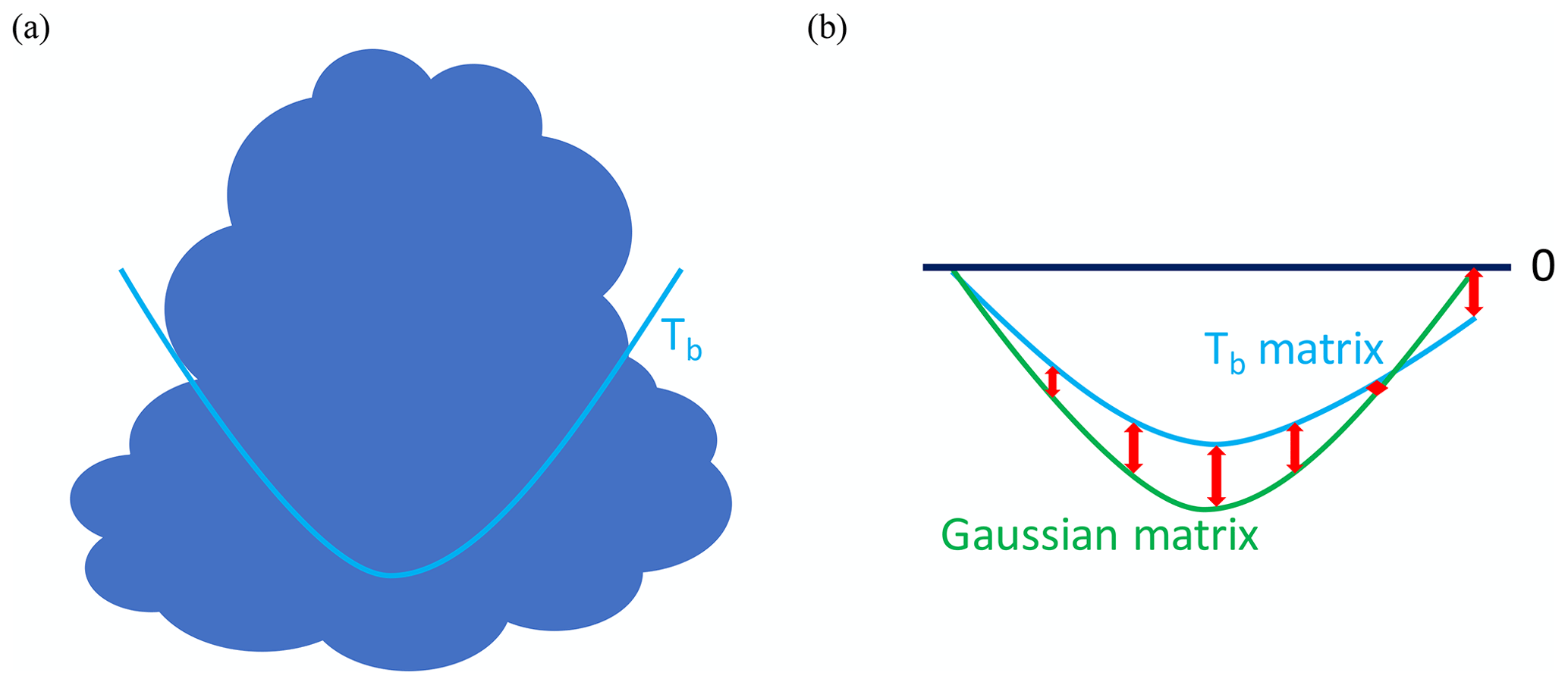
Figure 1(a) A typical shape of a convective cloud and its Tb distribution around the convective core (blue line). (b) Schematic representation of distributions of the upside down Gaussian matrix (green) and the Tb matrix (blue) when the cloud is convective.
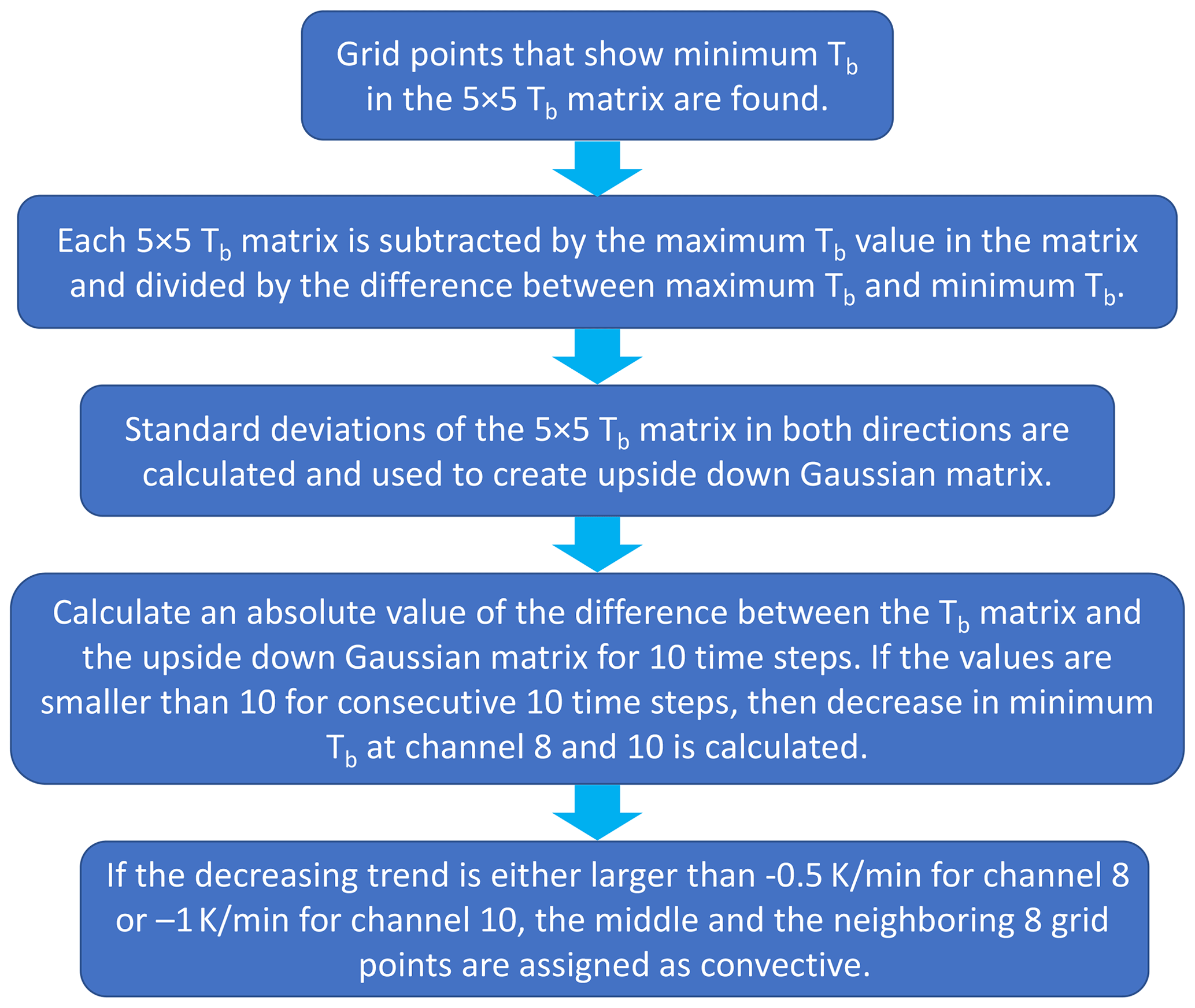
To compute the Tb decrease in clouds, a window has to be defined as it is usually difficult to precisely define the boundary of clouds, especially at the early stages of convection. Since most of the early convective clouds are smaller than 10 km in diameter, the window was defined as a 10 km × 10 km box which is essentially a 5 × 5 matrix of satellite pixels consisting of 25 Tb values with 2 km resolution. Considering the fact that a convective core usually has the lowest Tb within its neighborhood, the Tb matrix was formed around a pixel only if that pixel had the lowest Tb in the 5 × 5 matrix. However, this criterion alone could not distinguish convective cores from stratiform clouds and cloud edges which can also exhibit a local minimum. In addition to the lowest Tb, the shape of convective clouds is therefore also considered. As shown in the Fig. 1a, convective clouds not only have the lowest Tb in their cores in all directions, but also have increasing Tb values away from the core, making their Tb distributions look like an inverted two-dimensional (2D) Gaussian distribution. To select Tb matrices that have this upside down Gaussian shape, an inverted 5 × 5 Gaussian matrix that has mean and standard deviation of the Tb matrix was created and compared with the Tb matrices. To focus the comparisons on the shape of the Tb distribution (Fig. 1b), the maximum Tb found in the 5 × 5 matrix was subtracted from all values, and Tb values were divided by the difference between maximum and minimum Tb to normalize the Tb matrix itself. If the Tb matrix has a shape of a developing cloud (i.e., 2D upside down Gaussian), the absolute value of the difference between the Tb matrix and the upside down Gaussian matrix will be small. A threshold of 10 for this absolute value of the difference between Tb matrix and upside down Gaussian matrix (sum of residuals between normalized Tb and upside down Gaussian) was empirically determined to exclude non-convective scenes. Tb matrices with values greater than 10 are removed from the scene. This is done for all 10 consecutive Tb images that are 1 min apart. Continuous overlaps of Tb matrices for 10 min imply that the cloud maintained a convective shape for 10 min, and therefore changes in Tb are calculated to assess if the cloud in the Tb matrices was growing. The minimum Tb values of the Tb matrices at each time step were linearly regressed against time to measure a decreasing trend. If the fitted line at each channel had a slope either smaller than −1 K min−1 for Channel 10 or −0.5 K min−1 for Channel 8, the grid point with the lowest Tb at each time step for 10 min as well as the neighboring eight grid points in the window were classified as convective. This procedure is summarized in a flow chart in Fig. 2.
Table 1Number of non-convective, convective, convective within 10 min, and convective within 20 min for using different threshold values (Channel 8).
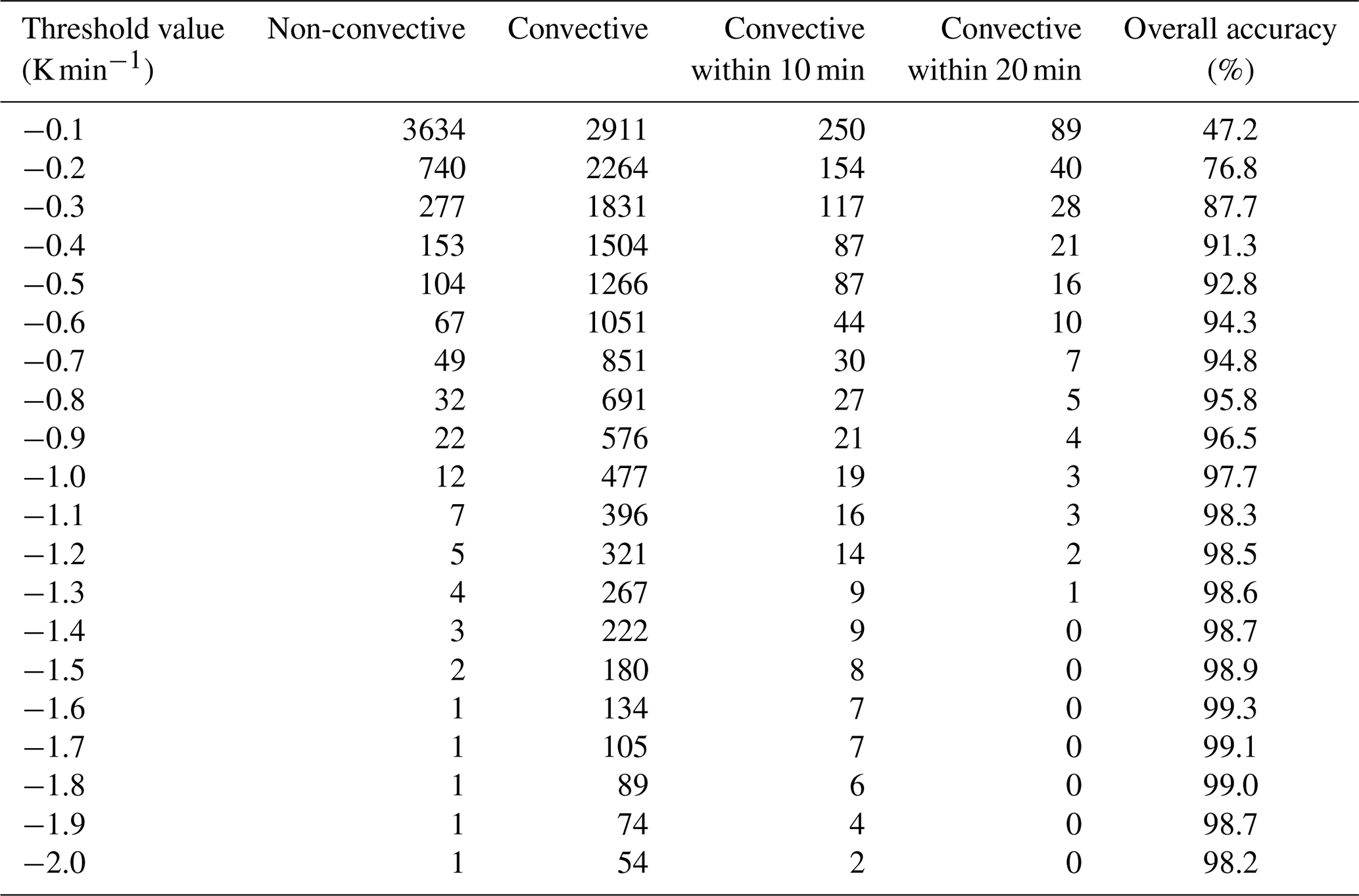
Table 2Number of non-convective, convective, convective within 10 min, and convective within 20 min for using different threshold values (Channel 10).
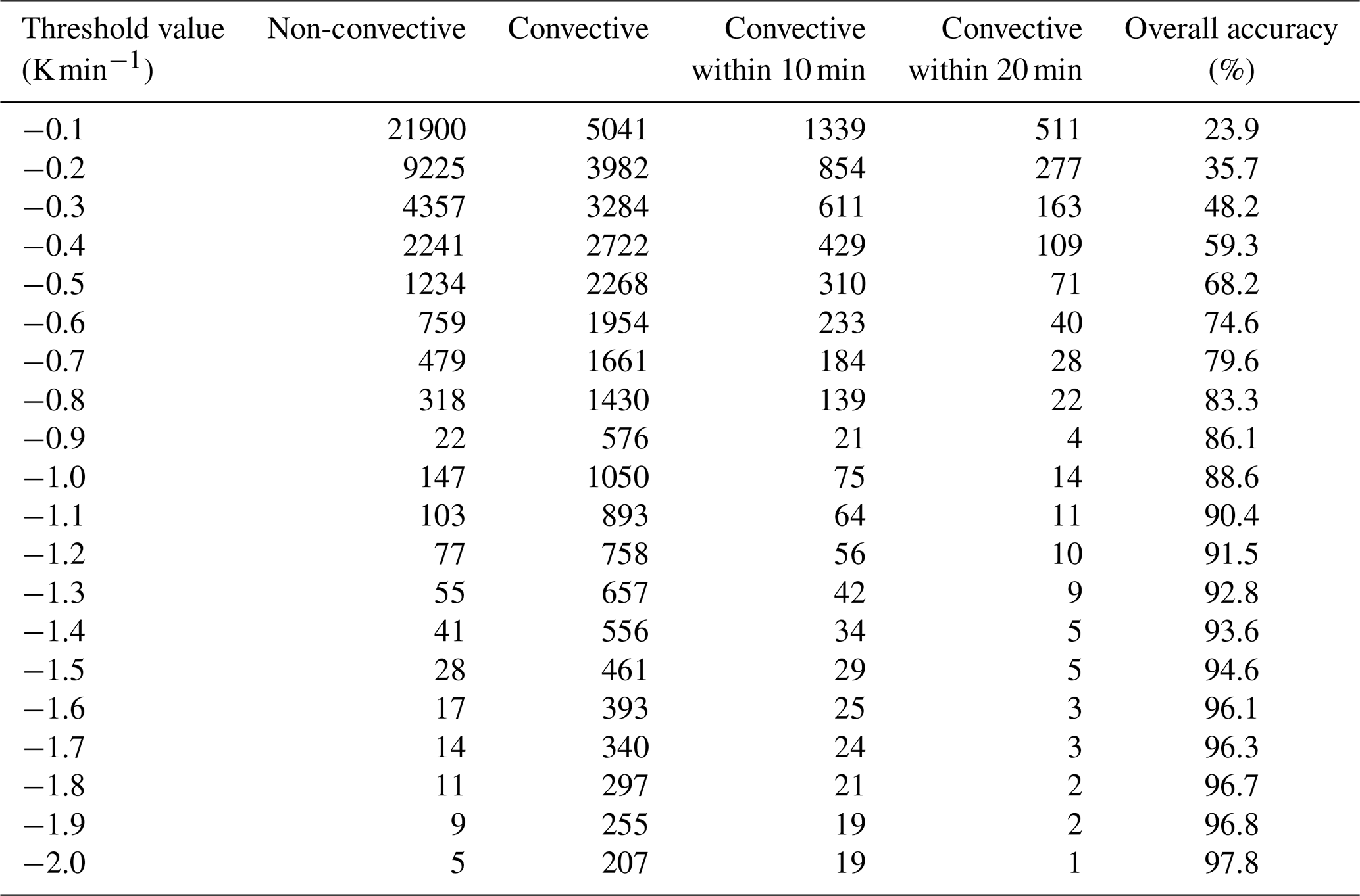
Water vapor channels have different sensitivity to water vapor, and thus different values for the threshold are chosen for each channel (Channels 8 and 10). Since growth rate can vary depending on the surrounding environment and different evolution stages, it is important to find an appropriate threshold that best represents the growth rate for clouds in their early stages. These thresholds are chosen based on the analysis of 1-month data during July of 2017. The 5 × 5 Tb windows that maintained the developing shape and had a decreasing trend of Tb during 10 min are collected over the 1-month period. A total of 38293 and 97042 (for Channels 8 and 10, respectively) 5 × 5 windows that show a decrease in Tb were collected, and precipitation types from MRMS were assigned for each window. Future MRMS convective flags up to 20 min after the detection period were included in the analysis because some time delays were observed in MRMS product when assigning convective flags, especially for early convection. When comparing GOES products to future MRMS products, future locations of GOES products were calculated assuming convection moves at the same speed at which clouds moved during the initial 10 min. Tables 1 and 2 show results applying different thresholds ranging from −0.1 to −2.0 K min−1. For each row, 5 pixel × 5 pixel windows that show a larger temperature decrease than the corresponding threshold are collected, and they are analyzed for potential convection. Numbers in the table represent the number of 5 × 5 windows that MRMS precipitation flags were assigned to either non-convective or convective at the corresponding 10 min time window, as well as pixels that were flagged as convective by MRMS in the next 10 and 20 min to account for the fact that GOES can detect convection before the radar sees precipitation. However, not all the detection by the method is done early since MRMS can also sometimes assign early convection as convective before it produces high reflectivity. The overall accuracy in the last column is calculated by dividing the number of windows that were convective within 20 min (sum of convective, convective within 10 min, and convective within 20 min) by the total number of the windows (sum of non-convective, convective, convective within 10 min, and convective within 20 min). Some convective clouds in the early stage show a smaller decreasing trend than the thresholds, but using a smaller value for the threshold can introduce clouds that do not grow into deep convective clouds in the end. Clouds that develop into deep convective clouds are eventually captured by these thresholds in later times as they show rapid intensification sooner or later. However, choosing a large cooling rate for the threshold will lead to less detection of convective clouds as not a lot of windows show a large cooling rate. Therefore, thresholds of −0.5 and −1.0 K min−1 for Channels 8 and 10, respectively, are chosen so that reasonable amounts of convections are detected. The cooling rate observed at Channel 8 is smaller than Channel 10 due to higher absorption at Channel 8. Channel 8 senses moisture at higher altitude, and thus when water vapor starts to condensate at lower levels, it is less affected, and its Tb does not decrease as much as in Channel 10. The matrix does not have to be detected at both channels, but using two channels tends to find the same vertically growing clouds over time by detecting the cloud using Channel 8 first and then using Channel 10 later. This method will be called the growing cloud detection method hereinafter.
Furthermore, it is interesting to note that some clouds did not produce precipitation even with rapid growth over −2.0 K min−1 (for Channel 10). This would be due to mixing between convective cells and their dry environment or the highly non-linear nature of chances of precipitation.
3.2 Detection of mature convective clouds with reflectance data
Mature convective clouds consist of convective cores and stratiform or cirrus regions where clouds have detrained from the core. The lack of discrete boundaries between different types of clouds makes it difficult to separate convective grid points from surrounding stratiform regions. Overshooting tops and enhanced-V pattern are well-known features in mature convective clouds, but these do not appear until their strongest stage and not in all convective clouds. Using such features associated with the deepest convective cores will create a detection gap between early and mature stages of convection. The method described here tries to minimize the gap, while still accurately detecting convective clouds.
Before evaluating the texture, only the grid points that are potentially parts of deep convection are selected using simple threshold values of VIS (ABI Channel 2; 0.65 µm) and IR (ABI Channel 14; 11.2 µm) channels. Channel 2 reflectance is highly correlated with the cloud optical depth (Minnis and Heck, 2012) while Channel 14 brightness temperature is related to cloud top temperature (Müller et al., 2018). These channels are used in GOES-R baseline product retrieval of cloud optical depth and cloud top properties, respectively. Any grid points with reflectance less than 0.8 or Tb greater than 250 K during 10 time steps (10 min) are removed since they generally represent thin or low clouds such as cirrus or growing clouds that can be identified by the CI method described earlier. These thresholds are chosen rather generously to include some convective clouds that have not grown into deep convection yet, while still avoiding the misclassification of low cumulus clouds and thin anvil clouds as convective. The threshold of 250 K is much warmer than typical values used in detecting deep convective features such as overshooting tops (Bedka et al., 2010) or enhanced V (Brunner et al., 2007). A warmer threshold is intentionally chosen so that the method considers warmer convective clouds without those features in the next step when evaluating lumpiness of the cloud top. The choice of these thresholds is discussed in more detail in Sect. 4.3.
Once cold, highly reflective scenes are identified, regions with bubbling cloud top are found. Bubbling cloud top is a distinct feature that appears in convective clouds, even in their early stages. The lumpiness of cloud tops can be numerically represented by calculating horizontal gradients in the reflectance field with the Sobel–Feldman (Sobel) operator which is commonly used in edge detection. The horizontal gradient is calculated at each pixel. The Sobel operator convolves the target pixel and its surrounding eight grid points with two kernels given in Eq. (1) to produce gradients in the horizontal and vertical direction.
By using Eq. (2), gradients in each direction are combined to provide the absolute magnitude of the gradient at each point.
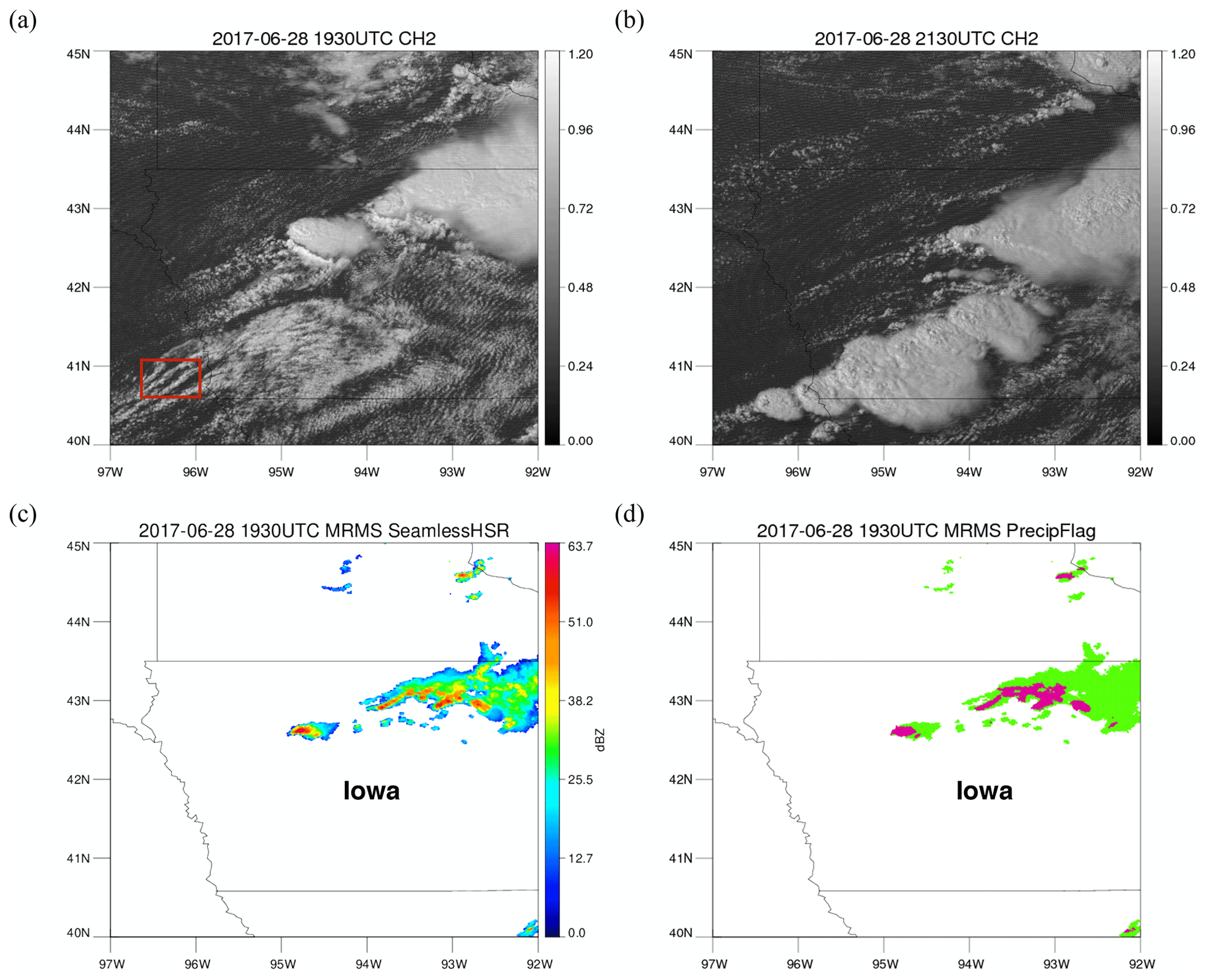
Figure 3(a) GOES-ABI 0.65 µm visible channel imagery (0.5 km) at 19:30 UTC on 28 June 2017 over Iowa. Numbers on the color bar represent reflectances. The red box indicates regions where two convective cells are detected by the growing cloud detection method. (b) GOES-ABI 0.65 µm visible channel imagery at 21:30 UTC on 28 June 2017. (c) MRMS Seamless Hybrid Scan Reflectivity (SHSR) at 19:30 UTC on 28 June 2017. (d) MRMS PrecipFlag at 19:30 UTC 28 June 2017. Pink represents convective while green represents stratiform.
Flat surfaces will have low gradients while cloud edges or lumpy surfaces will have high gradients. This lumpy feature is most evident in a VIS channel with the finest spatial resolution of 0.5 km. IR fields are not very useful as the brightness temperature variations in these lumpy surfaces tend to be quite small due to their relatively lower spatial resolution, and only cloud edges stand out.
The average of the horizontal gradients over the 10 1 min time steps is calculated for each grid point, and grid points are removed if the average was less than 0.4 or greater than 0.9. Values below 0.4 or above 0.9 generally imply either stratiform region with a flat surface or cloud edges with very high gradients, respectively. The thresholds are chosen to produce relatively low false alarms comparing results using other thresholds. Results using other thresholds are also shown in Sect. 4.3 for a comparison. The remaining grid points were then interpolated into 1 km maps to be consistent with the spatial resolution of the MRMS dataset. Neighboring grid points were grouped to form clusters, and only the clusters with more than five grid points were assigned as a mature convective cloud to remove noise. This method will be called the mature cloud detection method hereinafter.
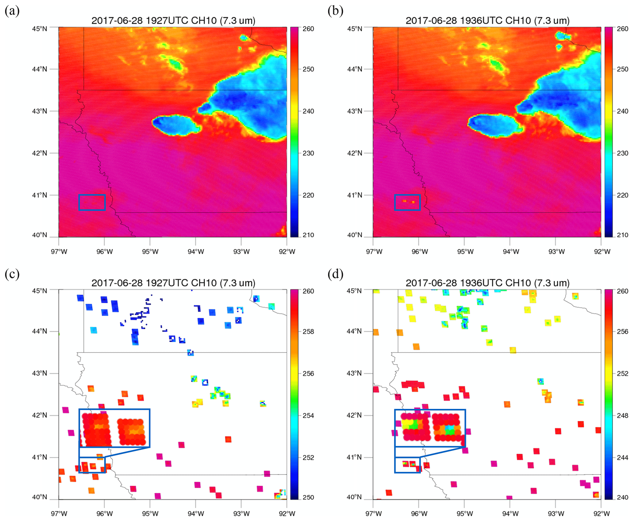
Figure 4(a) GOES-ABI 7.3 µm infrared channel imagery (K) at 19:27 UTC on 28 June 2017. Blue box denotes regions where two convective clouds start to grow. (b) Same as (a), but at 19:36 UTC. (c) Tb matrices obtained from Channel 10 (7.3 µm) that have the Gaussian shape at 19:27 UTC on 28 June 2017. Blue box denotes the same region as the blue box in (a). Note that the scale of the color bar is adjusted from (a, b) to better observe convective initiation. (d) Same as (c), but at 19:36 UTC.
4.1 28 June 2017
Supercell thunderstorms developed in Iowa and produced several tornado touchdowns. In Fig. 3a, deep convection had already developed over central Iowa at 19:30 UTC, and two convective cells in the red box started to develop in southwest Iowa, although they do not stand out from surrounding low clouds in the VIS image. These two convective clouds became parts of major storm system that formed around 21:30 UTC, producing the tornadoes (Fig. 3b) in the area. MRMS Seamless Hybrid Scan Reflectivity (SHSR), which gives reflectivity at the lowest possible vertical level, is shown in Fig. 3c, and the MRMS PrecipFlag product is shown in Fig. 3d. Convection is colored in pink and stratiform in green. Although deep convections over the central and northeast part of Iowa were assigned as convective in MRMS at 19:30 UTC, the two growing clouds in the red box in Fig. 3a were not assigned a convective flag until 19:48 UTC.
Figure 4a shows brightness temperatures for ABI Channel 10 (7.3 µm) at 19:27 UTC. The two growing convective cells in the blue box are shown in barely visible yellow surrounded by high Tb values. The one on the left was detected using 10 min data from 19:25 UTC, but since both clouds were detected together starting at 19:27 UTC, a scene from 19:27 UTC was used to demonstrate the method. Figure 4c and d show Tb matrices that exhibited the correct shape for developing cells (Gaussian shape) at 19:27 and 19:36 UTC. However, not all of the matrices in these figures showed the evolution of the developing cells (decreasing minimum Tb over 10 K) between the two time steps. The two matrices in the blue box satisfied both criteria of maintaining the shape of developing cells and growing vertically over 10 time steps while other matrices did not satisfy either one of the criteria. These two matrices contain early convective clouds that grow into deep convection shown in Fig. 3b, and they are correctly captured by this method.
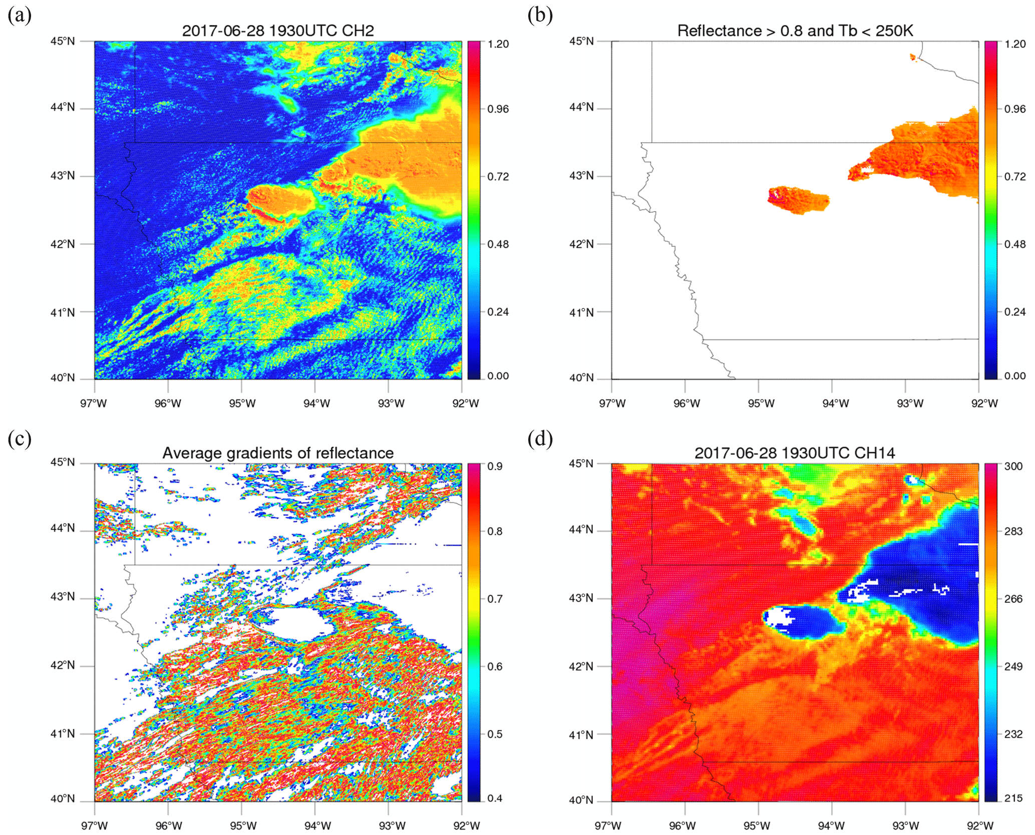
Figure 5(a) Same as Fig. 3a, but using different color table. (b) From the reflectance map in (a), regions that have reflectances over 10 min less than 0.8 or have Tb values greater than 250 K over 10 min are assigned reflectance of zero, and therefore colored in white. (c) Map of average gradients of reflectances over 10 min. Regions with average gradient less than 0.4 or greater than 0.9 are colored in white. (d) GOES-ABI 11.2 µm infrared channel imagery (K) at 19:30 UTC on 28 June 2017. Regions that passed two criteria from (b) and (c) are colored in white.
Results for the detection of mature convective clouds are shown in a step-by-step fashion in Fig. 5. Figure 5a is the same as in Fig. 3a but is mapped using a different color table for better comparisons between steps. Figure 5b shows the pixels retained after eliminating all the grid points that did not meet the reflectance and Tb thresholds (minimum reflectance over 10 time steps greater than 0.8 and maximum Tb over 10 time steps less than 250 K). Figure 5c shows the horizontal gradient values after applying the Sobel operator. The color bar is set to be within the range of 0.4 and 0.9 to display potential convective regions that passed these thresholds in colors. White regions are either regions that have average gradients greater than 0.9 such as cloud edges or thin cirrus clouds, or regions that have average gradients less than 0.4 such as clear sky or stratiform regions. Eventually, only the regions that meet the criteria in both Fig. 5b and c are assigned to convection and shown as white shading in Fig. 5d. Using a reflectance threshold sometimes limits the detection of shaded convective regions that exhibits lower reflectance than the threshold of 0.8. This is the case for the small imbedded white regions in the midst of high-reflectance regions shown in Fig. 5b. However, these regions are relatively small, and once they are upsampled into 2 km maps through nearest-neighbor interpolation, some of these regions are included in the detection as shown in Fig. 5d.
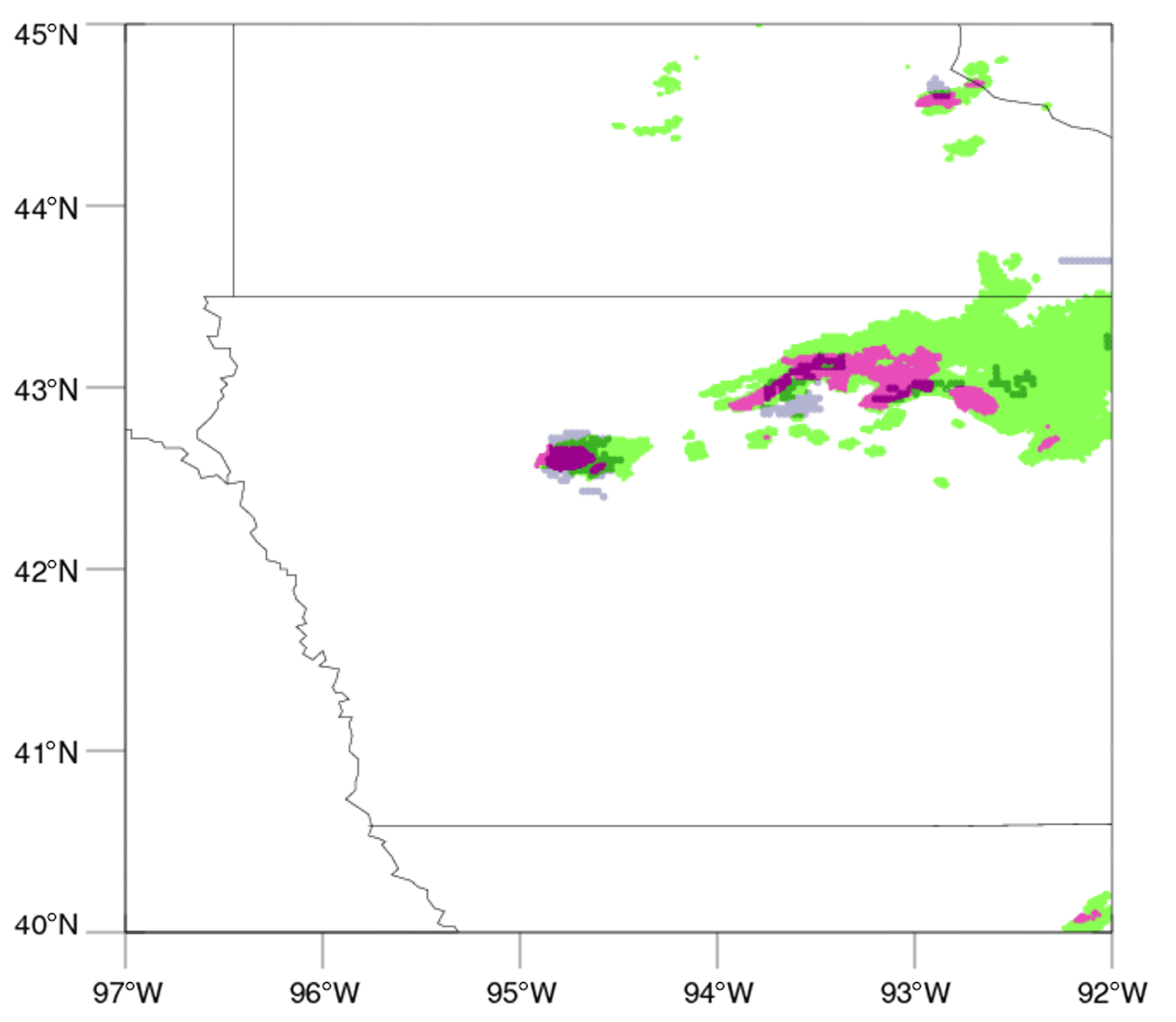
Figure 6Convective regions detected by GOES-16 (white regions in Fig. 5d) are colored in navy on top of MRMS PrecipFlag at 19:30 UTC on 28 June 2017. (Same figure as Fig. 3d. Pink represents convective while green represents stratiform.)
Detection from GOES and MRMS is compared in MRMS's resolution of 1 km, and in such high resolution, the location of a cloud seen from GOES and MRMS can be slightly different due to parallax displacement. For a better comparison between detection from GOES and MRMS, parallax correction based on Vicente et al. (2002) is applied to GOES detection using a constant cloud top height of 10 km. Convective regions detected by GOES (Fig. 5d) are plotted with the parallax correction on top of the MRMS map (Fig. 3d), and it is shown in Fig. 6. When compared to high-reflectivity regions in Fig. 3c and convective regions in Fig. 3d, convective regions, while not perfectly aligned due to a number of dynamic geometric reasons, do have a high degree of correspondence between the two detection methods. However, a straight line around 43.7∘ N at the right edge of Fig. 5d is definitely not a convective region, and it is due to unrealistically high reflectance in the raw satellite dataset. These kinds of artifacts were removed later in Sect. 4.3 when the method was applied to a full month of data. However, multiple lines are difficult to remove at this stage in the processing and will result in false alarm. As quality control procedures on ABI are improved, this may no longer be a source of significant errors.
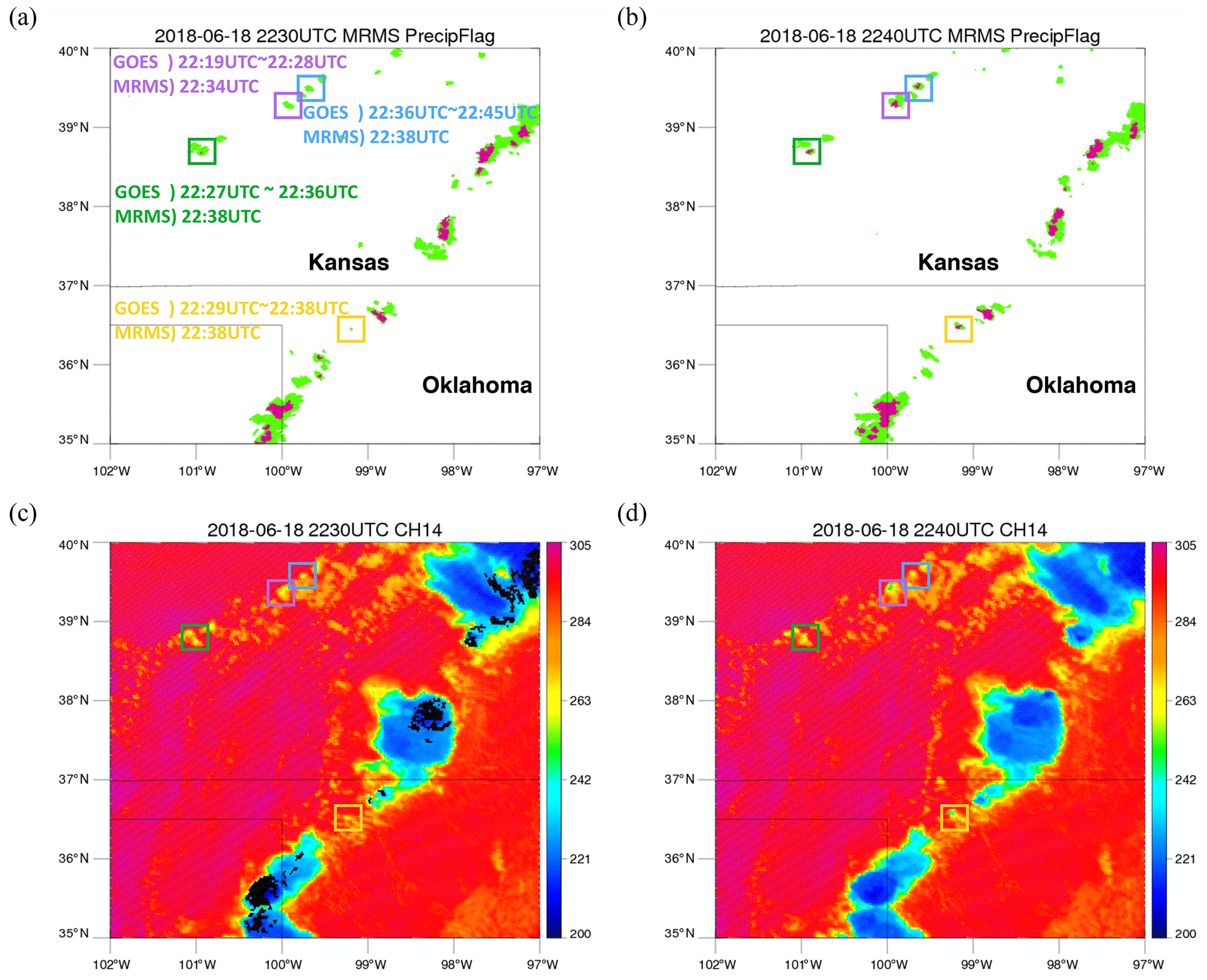
Figure 7(a) MRMS PrecipFlag at 22:30 UTC on 18 June 2018. Pink represents convective while green represents stratiform. Times next to each box represent the times of GOES data used in the growing cloud detection method and time of detection by MRMS. (b) MRMS PrecipFlag at 22:40 UTC on 18 June 2018. (c) GOES-ABI 11.2 µm infrared channel imagery (K) at 22:30 UTC on 18 June 2018 over the Great Plains. (d) Same as (c), but at 22:40 UTC.
4.2 18 June 2018
Another case was examined to evaluate the methods under different conditions. Severe storms developed over the Great Plains in 18 June 2018, producing hail on the ground. At 22:30 UTC, sporadic storms across Kansas and Oklahoma were observed by GOES-16. This scene contains both growing and mature convective clouds that are detected by MRMS during the 22:30–22:40 UTC period. In particular, four vertically growing clouds in this scene show different evolution and thus allow more elaboration on the growing cloud detection method. MRMS PrecipFlag for the scene at 22:30 and 22:40 UTC is shown in Fig. 7a and b, respectively. The green color represents stratiform and the pink color represents convective clouds. Figure 7c and d are Tb maps of the same scene at 22:30 and 22:40 UTC, respectively. Growing clouds shown in purple, blue, yellow, and green boxes are detected by the growing cloud detection method, but all starting from different time. Times that each cloud is detected by GOES and MRMS are shown in Fig. 7a. Time for the growing cloud detection method is a period as the method uses 10 consecutive 1 min data. Convection in the purple box was detected 6 min earlier than MRMS detection considering the last data used in the growing cloud detection method at 22:28 UTC. Similarly, a cloud in the green box was detected a little earlier by GOES than MRMS. The growing cloud in the yellow box was detected at the same time by GOES and MRMS. On the other hand, the growing cloud in the blue box was detected later than MRMS detection at 22:38 UTC. This cloud did not grow rapidly enough during 22:30–22:40 UTC period as shown in Tb maps of Fig. 7c and d and did not meet the Tb threshold for Channel 10 at the onset of convection. However, it was detected by Channel 8 as it grew higher altitudes. This shows that a cloud that initially did not show high growth rate can have high growth rate as it vertically grows and can be detected by Channel 8 later in time. These results show that even though the thresholds for the growing cloud detection method can miss some convective clouds that grow slowly in the beginning, the thresholds were adequate for detecting rapidly growing convective storms which are of more interest during the forecast.
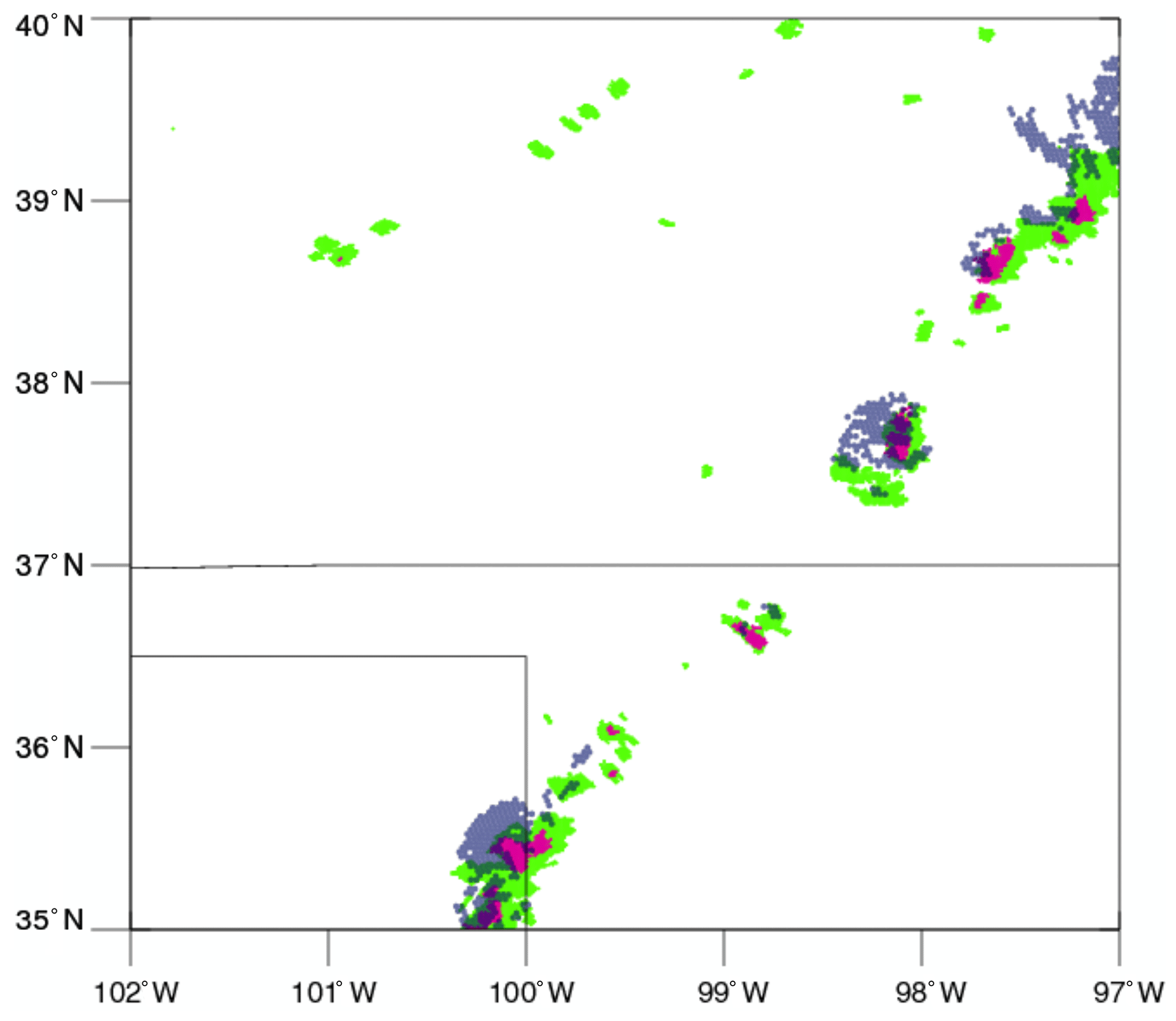
Figure 8Convective regions detected by GOES-16 (in Fig. 7c) are colored in navy on top of MRMS PrecipFlag at 22:30 UTC on 18 June 2018 (Fig. 7a). Pink represents convective while green represents stratiform).
Black regions superimposed on the brightness temperature map in Fig. 7c represent convective regions identified by the mature convection method, and Fig. 8 shows a figure of the black regions overlaid on top of the MRMS PrecipFlag map (Fig. 7a). There are slight misalignments of detected convective clouds between MRMS PrecipFlag products and GOES results possibly due to sheared vertical structures of the storms. One other thing to note here is that the convective area detected by the mature cloud detection method is greater than what is detected in the previous case. This could be due to the dependency of lumpiness on some geometrical considerations. Lumpiness is a function of the pixel spatial resolution, differences in optical depth, and shadows. Spatial resolution decreases away from the Equator, but higher solar zenith angles (due to altitude or time of day) not only increases optical depth, they also increase shadows. While this can of course be dealt with, it was ignored in this study which serves primarily as a proof of concept, as the method generally finds the convective core correctly.
Table 3Contingency table of results applying both of GOES detection methods and validating against MRMS data during June of 2017. Pixel-based validation is conducted to produce this table. C and NC represent convective and non-convective, respectively. GOES-C/MRMS-C denotes “hits” that both MRMS and GOES methods detected as convective within 5 km. GOES-NC/MRMS-C denotes “misses” that GOES missed detecting convection while MRMS assigned as convective. GOES-C/MRMS-NC denotes “false alarm” that GOES detected as convective, but MRMS did not. GOES-NC/MRMS-NC denotes a “correct negative case” that neither MRMS nor GOES detected as convective. Percentages in the parenthesis are obtained by dividing each number by the total number.

4.3 Statistical results with 1-month data
Pixel-based validation of the two methods is conducted using 1 month of data measured during June 2017. Results are validated against MRMS data as ground-based radar is used to detect convective regions during the short-term forecast, and precipitation is a rather direct indicator of convection in all stages. Since MRMS detection comprises convection in all stages, MRMS data are compared with GOES detection combining the two methods. Table 3 is a contingency table applying both methods to 1-month data and comparing in MRMS's grids with a spatial resolution of 1 km. C represents convection detected by either GOES or MRMS, and NC represents non-convective regions. GOES-C/MRMS-C is “hits” that both MRMS and GOES methods detected as convective within 5 km. In the case of the growing cloud detection method, on the other hand, hits are defined if MRMS assigned convective within 30 min due to earlier detection by this method. GOES-NC/MRMS-C denotes “misses” that GOES missed detecting convection while MRMS assigned as convective. GOES-C/MRMS-NC denotes a “false alarm” that GOES detected as convective, but MRMS did not. Lastly, GOES-NC/MRMS-NC denotes a “correct negative case” that neither MRMS nor GOES detected as convective. From the contingency table, verification metrics of probability of detection (POD) and false alarm rate (FAR) can be calculated as below.
POD and FAR are useful tools in evaluating detection skill of a binary problem. POD and FAR calculated from Table 3 are 45.3 % and 14.4 %. Since POD and FAR can vary depending on the thresholds used in each method, choosing different thresholds is examined further.

Figure 9Plot of probability of detection (POD) and false alarm ratio (FAR) using different texture thresholds of the mature cloud detection method. The Tb and reflectance thresholds are kept constant with 250 K and 0.8, respectively.
Most of the detection is from the mature cloud detection method as mature convective clouds account for a much larger area. The mature cloud detection method alone has FAR of 14.2 % and POD of 43.7 %. FAR and POD of the growing cloud detection method including 30 min data are 22.2 % and 3.9 %, respectively. Relatively small FAR compared to FAR from Tables 1 and 2 (1 − overall accuracy values) would be because Tables 1 and 2 are obtained based on each cloud while FAR and POD are calculated based on each grid point. Two PODs from the two methods (43.7 % and 3.9 %) do not add up to 45.3 % (POD calculated from Table 3) due to overlapped detection. Since the mature cloud detection method resort to several thresholds, results using different combinations of the three thresholds (reflectance at Channel 2 and Tb at Channel 14 to remove shallow and low clouds, and horizontal gradients of reflectance at Channel 2 to remove cloud edges as well as clouds with flat cloud top surfaces) are presented to show how they differ from the chosen thresholds. Two thresholds for cloud top texture, which are essentially horizontal gradients of reflectance, are evaluated first. The upper threshold does not change results much (not shown), and cloud edges are effectively removed by the threshold of 0.9. The lower bound of the texture thresholds are varied, keeping the upper threshold and the Tb and reflectance thresholds constant. Resulting FAR and POD are shown in Fig. 9. Using 0.5 (yellow) misses significant amounts of convective regions while using lower values (blue and red) substantially misclassifies stratiform regions with flat cloud tops as convective, although their PODs are much higher. Using 0.2 gives the closest results from the pixel-based validation in Zinner et al. 2013 using lightning data. However, FAR of 45.6 % when using 0.2 is no different from a random chance of 50 % that it is no longer useful, while POD of 29.9 % when using 0.5 will not give much information. Therefore, values of 0.4 and 0.9 (green diamond in Fig. 9) were chosen as a reasonable compromise between POD and FAR.
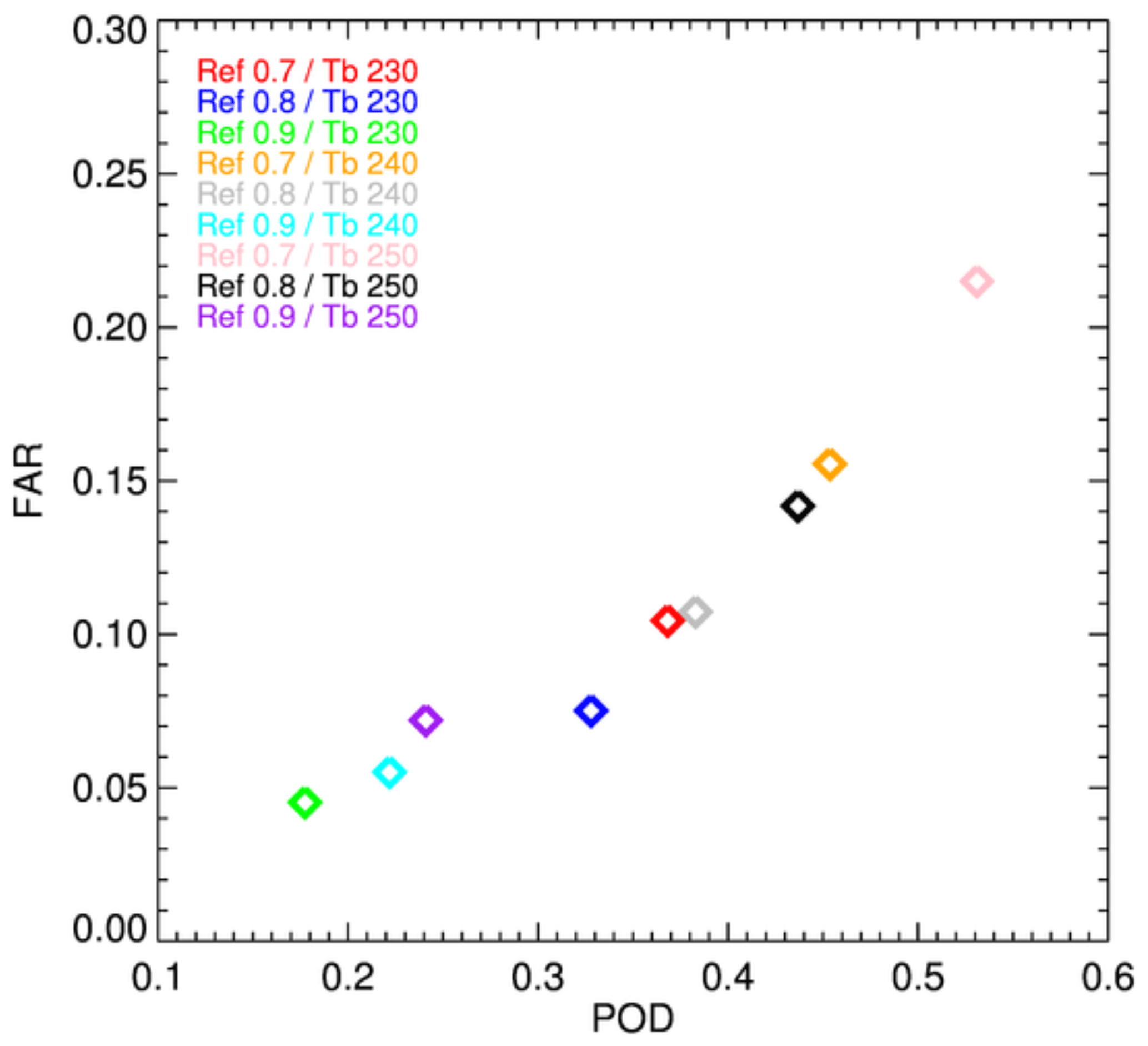
Figure 10Plot of probability of detection (POD) and false alarm ratio (FAR) for different combinations of Tb and reflectance thresholds. The texture threshold of 0.4 and 0.9 are kept constant.

Figure 11Histograms of Tb, reflectance, and texture values if a pixel was assigned to be convective by MRMS, but not detected by the mature cloud detection method due to each of the thresholds.
POD and FAR using different combinations of Tb and reflectance thresholds are plotted in Fig. 10, and this time texture thresholds are kept constant with 0.4 and 0.9. The Tb threshold is varied from 230 to 250 K, and the reflectance threshold is varied from 0.7 to 0.9. There is a trade-off between detecting more convective clouds that are transitioning into a mature stage and incorrectly assigning cumulus clouds as convective clouds. Having lower values for the Tb threshold or higher value for the reflectance threshold leads to small FAR, but also leads to small POD. To make this method effective and reduce FAR as much as possible for its potential use in the short-term forecast, 250 K for the Tb and 0.8 for the reflectance threshold (black diamond in Fig. 10a) are chosen. In data assimilation, it is preferable to provide no constraints than to provide the model with the incorrect location of convection. A value of 240 K and 0.7 (orange) also showed similar results, but 250 K and 0.8 were chosen due to lower FAR.
Despite its FAR being relatively small, the method misses significant amounts of convective areas observed by MRMS. Therefore, regions that were missed are evaluated further to investigate which threshold contributed most to missing those regions. Figure 11 shows histograms of Tb, reflectance, and texture in the convective regions that were missed by the above method. It is clear from the figure that the largest number of misses were due to low texture values (87.6 % of all missed regions has lower gradients than 0.4). There are many reasons why convective regions appear to have flat cloud top surfaces. Anvil or thick cirrus clouds above convective regions can smooth out or cover bubbling cloud tops, and there is simply no way to avoid this problem. Another reason may be the nature of the classification method. Since classification by MRMS is determined by rain rate, even if convective clouds are in a decaying mode and do not bubble anymore, clouds can still continue to precipitate considerable amounts, which would lead to convective category in the MRMS product. It is also possible that it is due to a misclassification of trailing stratiform regions using radars. There is indeed ongoing research in the radar community since a better convective and stratiform classification scheme improves QPE retrieval (Qi et al., 2013; Petković et al., 2019).
As shown from these results, there are no perfect thresholds that can separate convective and stratiform clouds. Nevertheless, threshold values were chosen in line with our main objective – to avoid high FAR as much as possible and have decent POD comparable to radar products. Avoiding FAR is a higher priority than reaching higher POD as giving false information is most detrimental during data assimilation. Low FAR of 14.4 % is achieved, and among those misclassified pixels, 96.4 % of them are at least raining. Since the main objective of data assimilation is to have good initialization of precipitation, applying these methods during data assimilation can still be beneficial in case the forecast model did not produce precipitation. Unfortunately, significant amounts of convective areas assigned by the radar product are missed. As shown in Fig. 11, most of the missed regions are excluded due to the flat surface, and this is an intrinsic problem of using VIS and IR bands. If a convective cloud is developing in a less cloudy scene, it can be detected by the method most of the time. However, in case of a hurricane where cloud tops are rather flat, or multi-layer clouds where cloud top information is decoupled from what is underneath, convection will be missed by the detection method. Furthermore, flat cloud top regions close to bubbling area might still be convective by MRMS due to high reflectivity, leading those regions to be classified as missed. The thresholds can be adjusted for other applications that may require higher POD.
This study explores two methods to detect convective clouds in two different stages using GOES-R ABI data with 1 min intervals. Using such high-temporal-resolution data facilitates cloud tracking in a more effective way and helps reduce uncertainties coming from cloud tracking when calculating decreases in Tb of the same cloud. Convective clouds in the early stage were detected using Tb values of ABI channels 8 and 10. These channels were used to find cloud scenes with the developing shape of convective clouds. They were then used again to calculate the Tb decrease for those which maintained the developing shape for 10 min. A cloud scene that had a consistent developing shape and a large decrease in Tb over 10 min was classified as convective by this method. Mature convective clouds were detected by masking out regions with high Tb in ABI Channel 14 and low reflectance in ABI Channel 2 and finding regions with high horizontal gradients of reflectance over the course of 10 min. Results from this mature cloud detection method were mostly consistent with the radar-derived products, although this method is limited to daytime use only. Nevertheless, it detects a wide range of convective area, not just regions with overshooting tops. Both methods are provided as a testing concept with several thresholds, and these thresholds can be tuned for an operational use if needed.
These methods work well for well-structured convective clouds, but there are limitations to this method, as with most algorithms using IR and VIS sensors. Cirrus cloud shields are the biggest problem as they block Tb decreases underneath and smooth out lumpy reflectance surfaces. However, these methods can still be useful for defining convection for assimilation into models where radar data are not available. Because regions identified as convective are most likely convective (∼ 85 % accuracy; 100 % − (FAR of 14.4 %)), this can easily be assimilated while setting cloudy regions to “missing” since the accuracy of detecting convection under large cirrus shields is poor. Furthermore, results using a Sobel operator, which is commonly used in image processing, implies that applying machine learning can be beneficial if the model can be set up to learn lumpy texture of convective clouds during training.
NEXRAD reflectivity data were obtained by NOAA's National Centers for Environmental Information: https://doi.org/10.7289/V5W9574V (NOAA National Weather Service (NWS) Radar Operations Center, 1991). Past MRMS datasets are available at http://mtarchive.geol.iastate.edu/ (last access: 2 May 2021, IEM Mtarchive, 2021). GOES-R data were made available by the Cooperative Institute for Research in the Atmosphere (CIRA).
All three authors designed the experiments. YL processed and analyzed the data. CDK and MZ gave feedbacks with their insights at every step of the data analysis. The paper was written jointly by YL, CDK, and MZ.
The authors declare that they have no conflict of interest.
This research is supported by CIRA's Graduate Student Support Program, as well as the WMO sponsored ICEPOP-18 project through the Korean Meteorological Administration.
This paper was edited by Bernhard Mayer and reviewed by two anonymous referees.
Ai, Y., Li, J., Shi, W., Schmit, T. J., Cao, C., and Li, W.: Deep convective cloud characterizations from both broadband imager and hyperspectral infrared sounder measurements, J. Geophys. Res., 112, 1700–1712, https://doi.org/10.1002/2016JD025408, 2017.
Autonès, F. and Claudon, M.: Algorithm Theoretical Basis Document for the Convection Product Processors of the NWC/GEO, available at : https://www.nwcsaf.org/ (last access: 2 May 2021), 2019.
Bauer, P., Thorpe, A., and Brunet, G.: The quiet revolution of numerical weather prediction, Nature, 525, 47–55, https://doi.org/10.1038/nature14956, 2015.
Bedka, K. and Khlopenkov, K.: A probabilistic multispectral pattern recognition method for detection of overshooting cloud tops using passive satellite imager observations, J. Appl. Meteorol. Clim., 55, 1983–2005, https://doi.org/10.1175/JAMC-D-15-0249.1, 2016.
Bedka, K., Brunner, J., Dworak, R., Feltz, W., Otkin, J., and Greenwald, T.: Objective satellite-based detection of overshooting tops using infrared window channel brightness temperature gradients, J. Appl. Meteorol., 49, 181–202, https://doi.org/10.1175/2009JAMC2286.1, 2010.
Bedka, K., Yost, C., Nguyen, L., Strapp, J. W., Ratvasky, T., Khlopenkov, K., Scarino, B., Bhatt, R., Spangenberg, D., and Palikonda, R.: Analysis and automated detection of ice crystal icing conditions using geostationary satellite datasets and in situ ice water content measurements, SAE International Journal of Advances and Current Practices in Mobility, 2, 35–57, https://doi.org/10.4271/2019-01-1953, 2019.
Benjamin, S. G., Weygandt, S. S., Brown, J. M., Hu, M., Alexander, C. R., Smirnova, T. G., Olson, J. B., James, E. P., Dowell, D. C., Grell, G. A., Lin, H., Peckham, S. E., Smith, T. L., Moninger, W. R., Kenyon, J. S., and Manakin, G. S.: A North American hourly assimilation and model forecast cycle: The rapid refresh, Mon. Weather. Rev., 144, 1669–1694, https://doi.org/10.1175/MWR-D-15-0242.1, 2016.
Bonavita, M., Trémolet, Y., Holm, E., Lang, S. T. K., Chrust, M., Janisková, M., Lopez, P., Laloyaux, P., de Rosnay, P., Fisher, M., Hamrud, M., and English, S.: A Strategy for Data Assimilation, Technical Memo, 800, ECMWF, Reading, UK, 2017.
Brunner, J. C., Ackerman, S. A., Bachmeier, A. S., and Rabin, R. M.: A quantitative analysis of the enhanced-V feature in relation to severe weather, Weather Forecast., 22, 853–872, https://doi.org/10.1175/WAF1022.1, 2007.
Churchill, D. D. and Houze Jr., R. A.: Development and structure of winter monsoon cloud clusters on 10 December 1978, J. Atmos. Sci., 41, 933–960, https://doi.org/10.1175/1520-0469(1984)041<0933:DASOWM>2.0.CO;2, 1984.
Cintineo, J. L., Pavolonis, M. J., Sieglaff, J. M., Wimmers, A., Brunner, J., and Bellon, W.: A Deep-Learning Model for Automated Detection of Intense Midlatitude Convection Using Geostationary Satellite Images, Weather Forecast., 35, 2567–2588, https://doi.org/10.1175/WAF-D-20-0028.1, 2020.
Dworak, R., Bedka, K., Brunner, J., and Feltz, W.: Comparison between GOES-12 overshooting-top detections, WSR-88D radar reflectivity, and severe storm reports, Weather Forecast., 27, 684–699, https://doi.org/10.1175/WAF-D-11-00070.1, 2012.
Geer, A., Ahlgrimm, M., Bechtold, P., Bonavita, M., Bormann, N., English, S., Fielding, M., Forbes, R., Hogan, R., Hólm, E., Janisková, M., Lonitz, K., Lopez, P., Matricardi, M., Sandu, I., and Weston, P.: Assimilating observations sensitive to cloud and precipitation, Technical Memo, 815, ECMWF, Reading, UK, 2017.
Gustafsson, N., Janjić, T., Schraff, C., Leuenberger, D., Weissman, M., Reich, H., Brousseau, P., Montmerle, T., Wattrelot, E., Bučánek, A., Mile, M., Hamdi, R., Lindskog, M., Barkmeijer, J., Dahlbom, M., Macpherson, B., Ballard, S., Inverarity, G., Carley, J., Alexander, C., Dowell, D., Liu, S., Ikuta, Y., and Fujita, T.: Survey of data assimilation methods for convective-scale numerical weather prediction at operational centres, Q. J. Roy. Meteor. Soc., 144, 1218–1256, https://doi.org/10.1002/qj.3179, 2018.
Han, D., Lee, J., Im, J., Sim, S., Lee, S., and Han, H.: A novel framework of detecting convective initiation combining automated sampling, machine learning, and repeated model tuning from geostationary satellite data, Remote Sens.-Basel, 11, 1454, https://doi.org/10.3390/rs11121454, 2019.
IEM Mtarchive: MRMS datasets, Iowa State University, US, available at http://mtarchive.geol.iastate.edu/, last access: 2 May 2021.
Jones, T. A., Knopfmeier, K., Wheatley, D., Creager, G., Minnis, P., and Palikonda, R.: Storm-scale data assimilation and ensemble forecasting with the NSSL experimental warn-on-forecast system. Part II: Combined radar and satellite data experiments, Weather Forecast., 31, 297–327, https://doi.org/10.1175/WAF-D-15-0107.1, 2016.
Lee, S., Han, H., Im, J., Jang, E., and Lee, M.-I.: Detection of deterministic and probabilistic convection initiation using Himawari-8 Advanced Himawari Imager data, Atmos. Meas. Tech., 10, 1859–1874, https://doi.org/10.5194/amt-10-1859-2017, 2017.
Mecikalski, J. R. and Bedka, K.: Forecasting convective initiation by monitoring the evolution of moving cumulus in daytime GOES imagery, Mon. Weather Rev., 134, 49–78, https://doi.org/10.1175/MWR3062.1, 2006.
Merk, D. and Zinner, T.: Detection of convective initiation using Meteosat SEVIRI: implementation in and verification with the tracking and nowcasting algorithm Cb-TRAM, Atmos. Meas. Tech., 6, 1903–1918, https://doi.org/10.5194/amt-6-1903-2013, 2013.
Migliorini, S., Lorenc, A. C., and Bell, W.: A moisture-incrementing operator for the assimilation of humidity and cloud-sensitive observations: formulation and preliminary results. Q. J. Roy. Meteor. Soc., 144, 443–457, https://doi.org/10.1002/qj.3216, 2018.
Minnis P. and Heck, P. W.: GOES-R Advanced Baseline Imager (ABI) Algorithm theoretical basis document for nighttime cloud optical depth, cloud particle size, cloud ice water path, and cloud liquid water path, National Oceanic and Atmospheric Administration (NOAA), available at: https://www.goes-r.gov/products/baseline-cloud-opt-depth.html (last access: 2 May 2021), 2012.
Müller, R., Haussler, S., and Jerg, M.: The role of NWP filter for the satellite based detection of cumulonimbus clouds, Remote Sens.-Basel, 10, 386, https://doi.org/10.3390/rs10030386, 2018.
Müller, R., Haussler, S., Jerg, M., and Heizenreder, D.: A Novel Approach for the Detection of Developing Thunderstorm Cells, Remote Sens.-Basel, 11, 443, https://doi.org/10.3390/rs11040443, 2019.
NOAA National Weather Service (NWS) Radar Operations Center: NOAA Next Generation Radar (NEXRAD) Level 2 Base Data, NOAA National Centers for Environmental Information [data set], https://doi.org/10.7289/V5W9574V, 1991.
Petković, V., Orescanin, M., Kirstetter, P., Kummerow, C., and Ferraro, R.: Enhancing PMW satellite precipitation estimation: detecting convective class, J. Atmos. Ocean. Tech., 36, 2349–2363, https://doi.org/10.1175/JTECH-D-19-0008.1, 2019.
Qi, Y., Zhang, J., and Zhang, P.: A real-time automated convective and stratiform precipitation segregation algorithm in native radar coordinates. Q. J. Roy. Meteor. Soc., 139, 2233–2240, https://doi.org/10.1002/qj.2095, 2013.
Scheck, L., Weissmann, M., and Bach, L.: Assimilating visible satellite images for convective-scale numerical weather prediction: A case-study, Q. J. Roy. Meteor. Soc., 146, 3165–3186, https://doi.org/10.1002/qj.3840, 2020.
Schmit, T. J., Griffith, P., Gunshor, M. M., Daniels, J. M., Goodman, S. J., and Lebair, W. J.: A closer look at the ABI on the GOES-R Series, B. Am. Meteorol. Soc., 98, 681–698, https://doi.org/10.1175/BAMS-D-15-00230.1, 2017.
Setvák, M., Rabin, R. M., and Wang, P. K.: A real-time automated convective and stratiform precipitation segregation algorithm in native radar coordinates, Q. J. Roy. Meteor. Soc., 139, 2233–2240, https://doi.org/10.1002/qj.2095, 2007.
Sieglaff, J. M., Cronce, L. M., Feltz, W. F., Bedka, K., Pavolonis, M. J., and Heidinger, A. K.: Nowcasting convective storm initiation using satellite-based box-averaged cloud-top cooling and cloud-type trends, J. Appl. Meteorol. Clim., 50, 110-126, https://doi.org/10.1175/2010JAMC2496.1, 2011.
Schmit, T. J., Griffith, P., Gunshor, M. M., Daniels, J. M., Goodman, S. J., and Lebair, W. J.: A closer look at the ABI on the GOES-R series, B. Am. Meteorol. Soc., 98, 681–698, https://doi.org/10.1175/BAMS-D-15-00230.1, 2017.
Steiner, M., Houze Jr., R. A., and Yuter, S. E.: Climatological characterization of three-dimensional storm structure from operational radar and rain gauge data, J. Appl. Meteorol., 34, 1978–2007, https://doi.org/10.1175/1520-0450(1995)034<1978:CCOTDS>2.0.CO;2, 1995.
Vicente, G. A., Davenport, J. C., and Scofield, R. A.: The role of orographic and parallax corrections on real time high resolution satellite rainfall rate distribution, Int. J. Remote Sens., 22, 221–230, https://doi.org/10.1080/01431160010006935, 2002.
Weygandt, S. S., Alexander, C. R., Dowell, D. C., Hu, M., James, E. P., Benjamin, S. G., Smirnova, T. G., Lin, H., Kenyon, J., and Olson, J. B.: Radar data assimilation impacts in the RAP and HRRR models, 20th Conf. on Integrated Observing and Assimilation Systems for the Atmosphere, Oceans, and Land Surface (IOAS-AOLS), New Orleans, Louisiana, USA, 10–14 January 2016, Amer. Meteor. Soc., available at https://ams.confex.com/ams/96Annual/webprogram/Paper289787.html (last access: 2 May 2021), 2016.
Yano, J.-I., Ziemiański, M. Z., Cullen, M., Termonia, P., Onvlee, J., Bengtsson, L., Carrassi, A., Davy, R., Deluca, A., Gray, S. L., Homar, V., Köhler, M., Krichak, S., Michaelides, S., Phillips, V. T. J., Soares, P. M. M., and Wzszogrodzki, A. A.: Scientific challenges of convective-scale numerical weather prediction, B. Am. Meteorol. Soc., 99, 699–710, https://doi.org/10.1175/BAMS-D-17-0125.1, 2018.
Zhang, J. and Qi, Y.: A real-time algorithm for the correction of brightband effects in radar-derived QPE, J. Hydrometeorol., 11, 1157–1171, https://doi.org/10.1175/2010JHM1201.1, 2010.
Zhang, J., Langston, C., and Howard, K.: Brightband identification based on vertical profiles of reflectivity from the WSR-88D, J. Atmos. Ocean. Tech., 25, 1859–1872, https://doi.org/10.1175/2008JTECHA1039.1, 2008.
Zhang, J., Howard, K., Langston, C., Kaney, B., Qi, Y., Tang, L., Grams, H., Wang, Y., Cocks, S., Martinaitis, S., Arthur, A., Cooper, K., Brogden, J., and Kitzmiller, D.: Multi-Radar Multi-Sensor (MRMS) quantitative precipitation estimation: Initial operating capabilities, B. Am. Meteorol. Soc., 97, 621–638, https://doi.org/10.1175/BAMS-D-14-00174.1, 2016.
Zhang, X., Wang, T., Chen, G., Tan, X., and Zhu, K.: Convective clouds extraction from Himawari–8 satellite images based on double-stream fully convolutional networks, IEEE Geosci. Remote S., 17, 553–557, https://doi.org/10.1109/LGRS.2019.2926402, 2019.
Zinner, T., Forster, C., de Coning, E., and Betz, H.-D.: Validation of the Meteosat storm detection and nowcasting system Cb-TRAM with lightning network data – Europe and South Africa, Atmos. Meas. Tech., 6, 1567–1583, https://doi.org/10.5194/amt-6-1567-2013, 2013.