the Creative Commons Attribution 4.0 License.
the Creative Commons Attribution 4.0 License.
 | 28 Jul 2021
GNSS-based water vapor estimation and validation during the MOSAiC expedition
Benjamin Männel
Florian Zus
Galina Dick
Susanne Glaser
Maximilian Semmling
Kyriakos Balidakis
Jens Wickert
Marion Maturilli
Sandro Dahlke
Harald Schuh
Within the transpolar drifting expedition MOSAiC (Multidisciplinary drifting Observatory for the Study of Arctic Climate), the Global Navigation Satellite System (GNSS) was used among other techniques to monitor variations in atmospheric water vapor. Based on 15 months of continuously tracked GNSS data including GPS, GLONASS and Galileo, epoch-wise coordinates and hourly zenith total delays (ZTDs) were determined using a kinematic precise point positioning (PPP) approach. The derived ZTD values agree to 1.1 ± 0.2 mm (root mean square (rms) of the differences 10.2 mm) with the numerical weather data of ECMWF's latest reanalysis, ERA5, computed for the derived ship's locations. This level of agreement is also confirmed by comparing the on-board estimates with ZTDs derived for terrestrial GNSS stations in Bremerhaven and Ny-Ålesund and for the radio telescopes observing very long baseline interferometry in Ny-Ålesund. Preliminary estimates of integrated water vapor derived from frequently launched radiosondes are used to assess the GNSS-derived integrated water vapor estimates. The overall difference of 0.08 ± 0.04 kg m−2 (rms of the differences 1.47 kg m−2) demonstrates a good agreement between GNSS and radiosonde data. Finally, the water vapor variations associated with two warm-air intrusion events in April 2020 are assessed.
- Article
(3123 KB) - Full-text XML
- BibTeX
- EndNote


Troposphere delays are generally regarded as one of the primary error sources in Global Navigation Satellite System (GNSS) positioning and therefore get modeled and estimated in the GNSS analysis process. By estimating these delays, it is possible to use GNSS for high-precision positioning but also as a valuable tool to monitor the troposphere. Conventionally, the zenith total delay (ZTD) consists of two parts: the zenith hydrostatic delay (ZHD) and the zenith wet delay (ZWD). The zenith delays are connected to the individual satellite observations and the associated slant delays by dedicated mapping functions and depend – apart from the air-pressure-related (hydrostatic) part – on the partial water vapor pressure and therefore on the water vapor in the lower atmosphere (Elgered and Wickert, 2017). By estimating this wet part of the delay (i.e., the ZWD), GNSS observations allow to observe directly the amount of atmospheric water vapor which is an active and most abundant component of the climate system (Alshawaf et al., 2018; Rinke et al., 2019). Atmospheric water vapor plays an essential role in today's climate variations, accounts for 60 %–70 % of the greenhouse effect (Kiehl and Trenberth, 1997; Guerova et al., 2016) and is an important input parameter for numerical weather models (NWMs). In the generally dry Arctic, atmospheric moisture intrusions from lower latitudes affect the snow and sea ice cover by increased longwave radiation (Woods and Caballero, 2016). The estimation of ZTDs and the subsequent conversion into precipitable water vapor (PWV) or integrated water vapor (IWV) is done operationally for several hundred land-based GNSS stations and is confirmed to agree with conventional meteorological observations (e.g., Gendt et al., 2004; Shangguan et al., 2015; Steinke et al., 2015). According to Ning et al. (2016), the accuracy of GNSS-based IWV is at a level of 1–2 kg m−2. However, with a few exceptions, continuous and long-term GNSS-based water vapor time series over oceans are not available but are highly important for climate investigations. In the past, several authors investigated shipborne PWV retrieval and reported an agreement at the 2 mm level compared to radiosondes (Fujita et al., 2008) and at the 3 mm level compared to radiometer data (Rocken et al., 2005). Boniface et al. (2012) investigated the ability to determine mesoscale moisture fields from shipborne GNSS data over 4 months. Wang et al. (2019) studied a 20 d ship cruise in the Fram Strait and reported an agreement for the PWV of 1.1 mm compared to weather models and radiosondes. Based on the 4-month ship campaign, Shoji et al. (2017) reported the practical potential of kinematic precise point positioning (PPP) for water vapor monitoring over oceans worldwide with particular challenges during high-humidity conditions. Based on the large-scale EUREC4A campaign, Bosser et al. (2021) presented IWV solutions derived from GNSS receivers aboard the research vessel (RV) Atalante, RV Maria S. Merian and RV Meteor. Overall, they reported a good agreement with biases of ±2 kg m−2 with respect to numerical weather models and terrestrial GNSS stations. For this study, we derived a 15-month zenith total delay and water vapor time series between summer 2019 and autumn 2020 observed by a GNSS receiver installed aboard the German RV Polarstern (Alfred Wegener Institute, 2017) as part of the Multidisciplinary drifting Observatory for the Study of Arctic Climate (MOSAiC) expedition.
The main objective of the MOSAiC expedition was to investigate the complex climate processes of the central Arctic for improving global climate models. RV Polarstern departed on 20 September 2019 from Tromsø, Norway, and started the transpolar drift on 4 October at 85∘ N, 137∘ E. Interrupted for around 4 weeks due to a supply trip to Svalbard in May and June 2020, RV Polarstern ended the drift on 9 August 2020 at 79∘ N, 4∘ E. For the second part of the expedition, RV Polarstern returned to the central Arctic in mid-August 2020 to observe the sea ice in its onset and early freezing phase. RV Polarstern finally returned to Bremerhaven on 12 October 2020. The GNSS receiver was a continuously operational instrument within the ship-based atmosphere monitoring system. It was provided by the GFZ German Research Centre for Geosciences with the main motivation to derive water vapor variations continuously from the ground and to allow a comparison for the radiosonde data.
Following this introduction, the GNSS installation on RV Polarstern and data availability is discussed in Sect. 2. The processing strategy applied in this study is summarized in Sect. 3, while Sect. 4 discusses the derived kinematic coordinates. In Sect. 5, the ZTD solution is assessed with respect to ERA5-based ZTDs and ZTDs derived from land-based GNSS and VLBI (very long baseline interferometry). Subsequently derived IWV values are discussed in Sect. 6 in comparison to preliminary radiosonde data. The paper closes with a summary and conclusions in Sect. 7.
The GNSS equipment was installed on 4 July 2019 shortly after the end of RV Polarstern's previous expedition PS120 and at the beginning of a nearly 6-week shipyard period. Consequently, GNSS data have been recorded during the stay at Bremerhaven, the PS121 expedition (Fram Strait) and the entire MOSAiC expedition (PS122). For logistical reasons, the receiver was switched off on 3 October 2020 at a position very close to Ny-Ålesund, Svalbard. Therefore, we have 15 months of high-accuracy GNSS data which are very valuable for climate relevant studies.
Figure 1 shows GFZ's GNSS equipment installed at RV Polarstern's observation deck. A JAV_GRANT-G3T antenna without a choke ring was used. To support reflectometry, the antenna was mounted on a cube structure together with a side-looking antenna (Semmling et al., 2021). The receiver equipment (geodetic JAVAD_TR_G3TH receiver) was stored in a cabinet mounted at the observation deck's railings. As visible in Fig. 1, the antenna location is not perfect as it is subject to shadowing and strong multipath effects caused by the nearby radomes and the crow's nest (i.e., the lookout point at the upper part of the mast). Due to limited data bandwidth during the cruise, data transfer in real time was not possible. Data post-processing started after the cruise at GFZ. The raw data were converted using the JPS2RIN converter software (version v.2.0.191). The derived RINEX (receiver independent exchange format) files were spliced, sampled and checked using gfzrnx (Nischan, 2016).
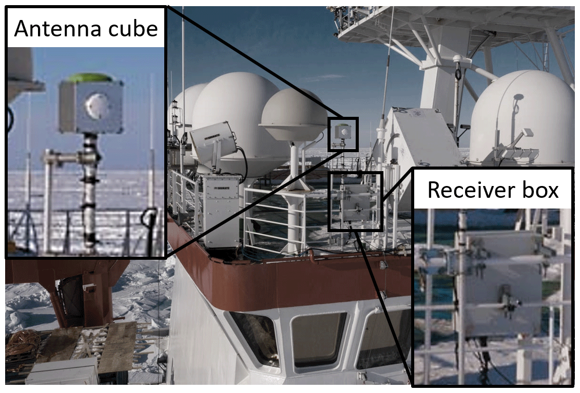
Figure 1RV Polarstern's observation deck in May 2020; the GFZ GNSS antenna is mounted at portside; courtesy Torsten Sachs (GFZ).
The considerably large number of received observations, represented in Fig. 2 in terms of L1 phase observations, is first of all promising. With a sampling rate of 30 s, around 1000 L1 phase observations were tracked per satellite and day over the complete time span of 15 months. Visible constellation-specific patterns are expected, as they are caused by the satellite orbit configurations, i.e., inclination, repeat cycle and revolution period.
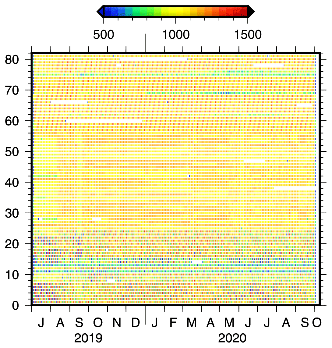
Figure 2Number of L1 observations (phase of first frequency) per day and satellite; observation types are L1X for Galileo (rows 1–25), L1W for GPS (rows 26–57), L1P for GLONASS (rows 58–82) for the GNSS receiver at RV Polarstern.
The Bernese GNSS Software v5.2 (Dach et al., 2015) was used for the data processing, which was performed as kinematic PPP (Zumberge et al., 1997) with epoch-wise estimated coordinates and hourly estimated zenith total delays among other parameters. The kinematic approach is needed to account for the traveling periods, height variations due to tides and waves, and the drift phases which showed an average speed of 12 km d−1 (corresponding to 4 m within the observation interval of 30 s). For validation purposes, the shipyard period in Bremerhaven (i.e., the dry dock period) was processed consistently in kinematic mode. The resulting kinematic coordinates are studied in Sect. 4. Overall, 25 ZTD values are estimated per day together with 8640 kinematic coordinates, 2880 clock corrections, around 80 differential code biases and around 280 ambiguities. The piecewise-linear ZTD estimates are constrained relatively with 1 mm. Table 1 provides a summary of the modeling and parametrization strategy. According to the capabilities of the processing software, ambiguity fixing was not applied. A low elevation cutoff angle of 3∘ was chosen to decorrelate ZTDs and coordinates. Larger cutoff angles were not tested related to the receiver's high latitude and the free horizon on the portside. An elevation-dependent observation weighting using cos 2(z) was applied with z as the zenith angle.
(Prange et al., 2020)(Böhm et al., 2006)(Rebischung and Schmid, 2016)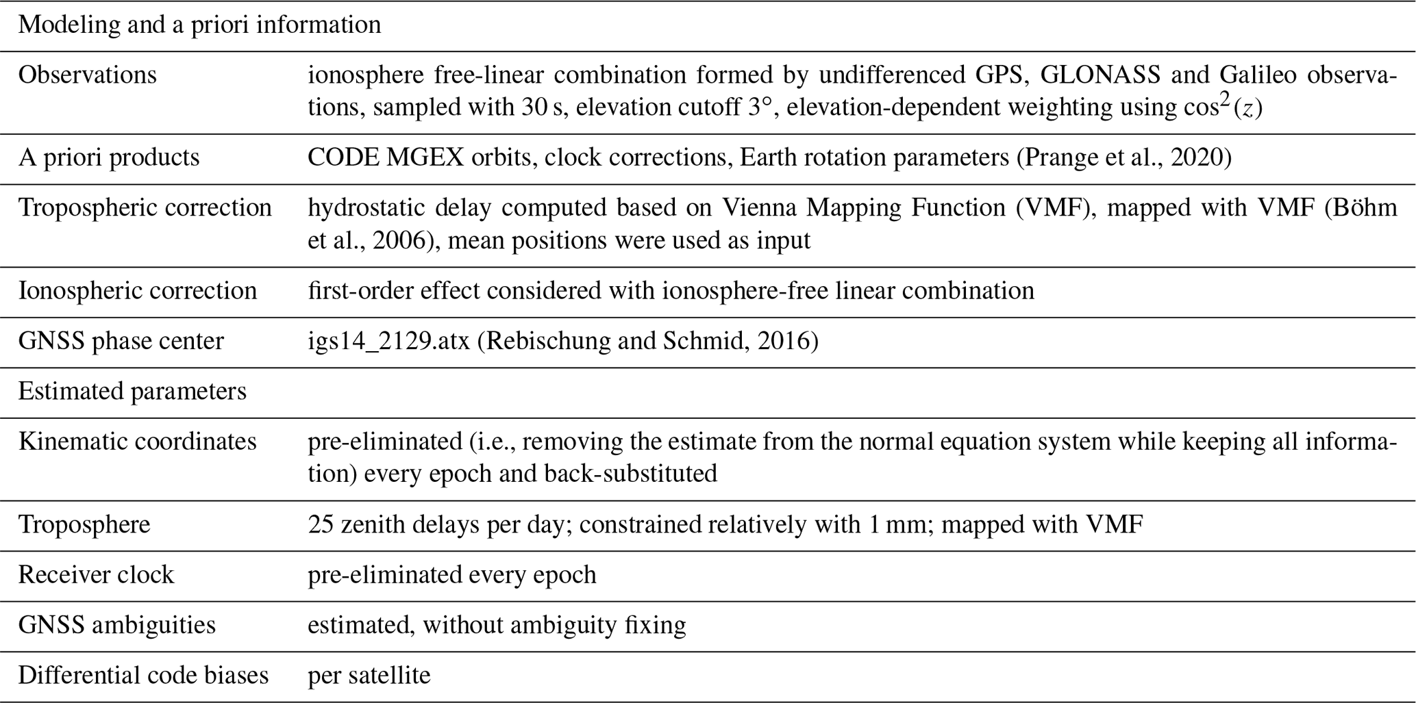
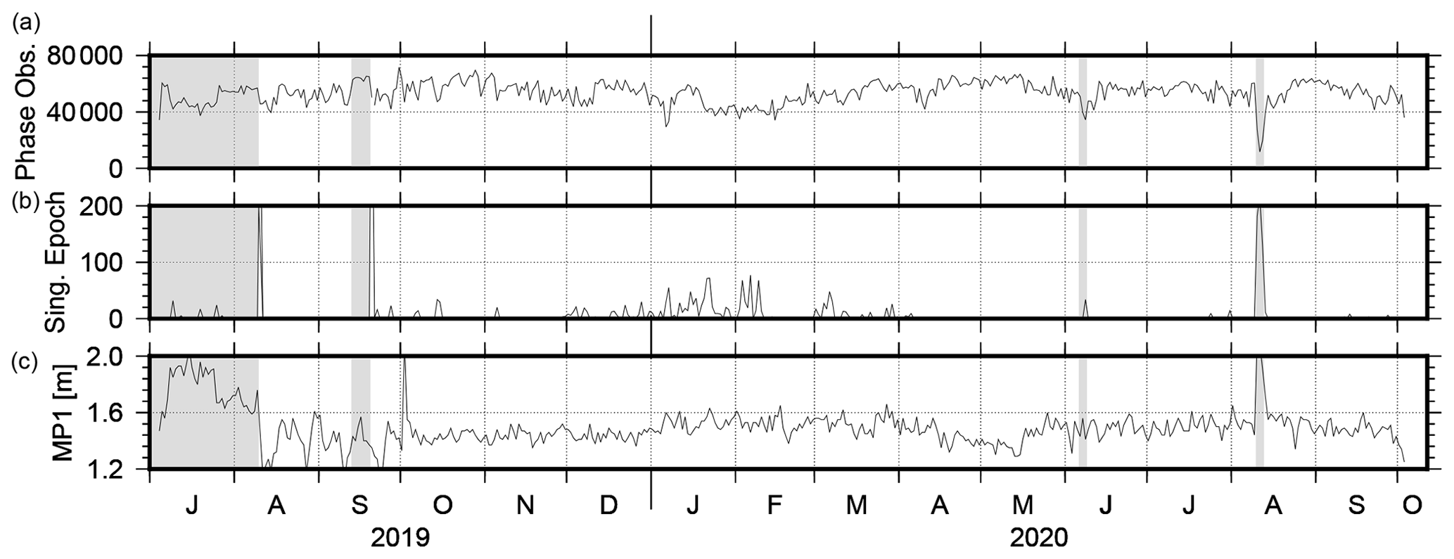
Figure 3Number of phase observations per day used in the final adjustment (a), number of singular epochs per day (i.e., epochs with fewer than four observations, based on 30 s sampling, b) and daily TEQC-based multipath MP1 values (c); periods of harbor stays and re-supply are shaded in gray.
Some general processing indicators are highlighted in Fig. 3. On average, 40 000 to 60 000 ionosphere-free observations remained after pre-cleaning for the daily processing, which is equivalent to 13–20 observations per epoch. As shown in the middle panel of Fig. 3, singular epochs, i.e., epochs with fewer than four observations, occurred for a number of days, mainly between December 2019 and March 2020. Due to the high latitude of the ship's position, satellite observations with very low elevations dominate during this period. Further signal delays are expected due to ice accumulation on the antenna and increased multipath effects caused by the surrounding instruments. The lower panel of Fig. 3 shows the MP1 multipath values derived from the RINEX files using TEQC (Estey and Meertens, 1999). Due to the antenna surrounding, large multipath effects of around 1.5 m occurred. According to Bosser et al. (2021), this value of 1.5 m is large compared to the multipath effects observed by RV Atalante and RV Meteor (in both cases, the GNSS antenna was installed at the crow's nest) but smaller than the multipath derived for RV Maria S. Merian, where the GNSS antenna was placed also on the observation deck. Between January and March 2020, the multipath effect increased by around 6 % compared to the previous 3 months. As visible in Fig. 3, a larger number of singular epochs occurred also during the port departures on 10 August 2019 (Bremerhaven, 381 epochs) and 20 September 2019 (Tromsø, 495 epochs); interestingly, this is not the case for the arrival in Tromsø. During the “refueling & personnel rotation 4” (10–12 August 2020), where RV Akademik Tryoshnikov was moored alongside RV Polarstern, the multipath parameter rose to values above 2 m, and the number of processed observations dropped below 30 000. The multipath parameter strongly increased due to additional reflections, especially as RV Akademik Tryoshnikov moored at RV Polarstern's port side. It can be noted that the MP1 values increased slightly during May 2020, which might be caused by additional equipment installed or stored at the observation deck, while RV Polarstern left the drift position. The number of singular epochs increased to 182, 216 and 129 epochs for the 3 d. Overall, these pre-processing results demonstrate and ensure precise and reliable results.
The processing strategy described above was defined with the focus on the post-processing approach required by the limited data bandwidth. However, a near-real-time processing which would allow a GNSS contribution to numerical weather prediction would be of course advantageous if an associated data link would be available. The processing strategy described in Gendt et al. (2004) could be applied in this case by additionally estimating kinematic coordinates. Consequently, ultra-rapid orbit products would be required as well as other a priori ZHD models and mapping functions. The quality of the derived ZTDs is expected to be almost similar to the results shown in this study.
In general, kinematic coordinates have to be estimated for a shipborne GNSS receiver to account for the ship's motion. Compared to static coordinates, kinematic coordinates cannot be assessed easily due to missing repetitions of positions (unlike the repeatability check for permanent stations) and the usual absence of any ground-truth information as, for example, known marker coordinates. Therefore, the assessment of kinematic coordinates is possible only during specific periods.
One specific period was during the shipyard stay in Bremerhaven, where RV Polarstern spent nearly 4 weeks in the dry dock and the antenna position could be assumed to be static and thus precisely assessed. Figure 4 shows the coordinate variations between 7 July and 3 August 2019 for the north, east and up directions. For the horizontal components, 79 % and 83 % of the coordinates are within ±4 cm. A larger variation is expected for the height with 78 % of the coordinates being within ±8 cm. The standard deviation of the derived horizontal coordinates is 4.8 and 5.7 cm for north and east, respectively. However, it has to be noted that during the shipyard stay, the multipath increased while the number of observations decreased significantly (see Fig. 3). This is most probably related to additional obstacles and reflections due to construction work. A mean ellipsoidal height of 61.49 ± 0.01 m was determined. Using a geoid height of 39.58 m at Bremerhaven, this corresponds to an antenna height of 21.91 m during the dry dock phases.
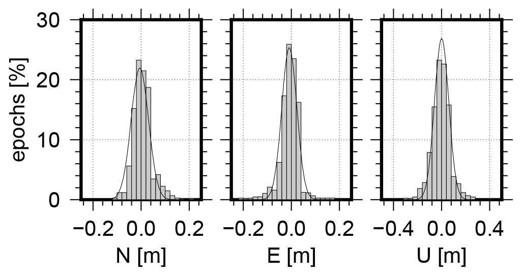
Figure 4Histogram of coordinate variations in the north, east and up directions for the dry dock period of RV Polarstern (7 July to 3 August 2019); a mean coordinate was subtracted; please note the different scales for horizontal and vertical components.
The second period for a coordinate validation is the harbor stay in Tromsø, Norway. Without a ship motion, the ocean tides can be used as ground truth; thus, the correlation between observed height and tidal record provides a validation opportunity. Figure 5 shows the GNSS-based height variations for 12 to 20 September 2019. A nearly perfect agreement compared to a close-by tidal record1 is visible with a correlation coefficient of 0.97 and a standard deviation of 20 cm. An empirically estimated height difference of 22.2 m is subtracted from the GNSS positions.
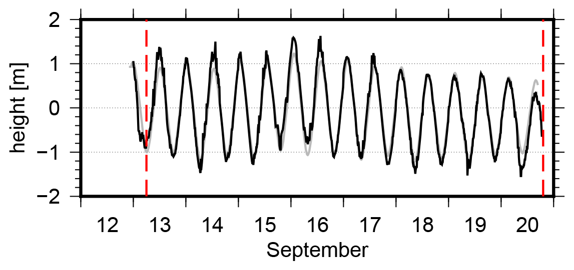
Figure 5Estimated height coordinates during the stay at Tromsø (black); the Tromsø tide gauge record is plotted for comparison (gray); an empirically estimated height difference of 22.2 m was subtracted from the GNSS positions; vertical red lines indicate RV Polarstern's arrival and departure times in Tromsø.
Overall, kinematic coordinates for nearly 1.3 million epochs were estimated from kinematic PPP, whereas 0.5 % of all epochs are singular (i.e., epochs with less than four satellites) and another 0.9 % are linearly interpolated but not estimated (see also Fig. 3), ensuring the high quality of the data.
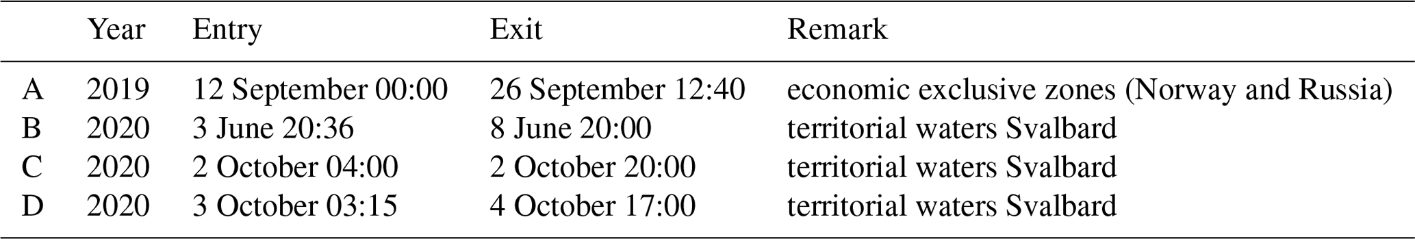
The derived ZTDs are analyzed and the results are presented in this section. The assessment and validation process includes the comparison to numerical weather model data (Sect. 5.1), a comparison against ZTD derived for selected onshore GNSS stations (Sect. 5.2) and to ZTD derived by VLBI at the radio telescopes in Ny-Ålesund (Sect. 5.3). During the entire 457 d, 10 973 unique ZTD values are estimated, i.e., 24 d−1, while the 25th value is computed for the first epoch of the following day. In accordance with the MOSAiC data guidelines and research agreements, water vapor results are restricted during (1) the harbor stay in Tromsø, (2) the subsequent passage of the economic exclusive zone of Norway and Russia, and (3) all periods within the territorial waters (12 nautical miles, 22 km) around Svalbard. Table 2 summarizes the affected periods. Following these restrictions, the number of investigated ZTDs is reduced to 10 503. Due to singular epochs, 54 ZTDs, and due to intervals with linearly interpolated coordinates, another 91 ZTDs (corresponding to 0.5 % and 0.8 % of all ZTDs) are excluded from the following statistics. In addition, ZTDs estimated for intervals with fewer than 800 observations are excluded (192 epochs, corresponding to 1.8 %). Overall, 10 166 GNSS-based ZTDs (96.8 %) are considered in the following comparisons. Related to the applied constraint, the formal errors of the remaining ZTDs are relatively small, with 99.6 % being below 4 mm.
Table 2List of restricted periods for which atmospheric measurements were not permitted. Time periods are given in UTC.
5.1 ZTD time series and comparison to ERA5
Figure 6 shows the ship track of RV Polarstern between August 2019 and October 2020. For clarity, the figure is split into two panels showing the periods of August 2019 to 5 June 2020 (left) and 6 June to 3 October 2020. The left panel shows the ZTD variations during the Fram Strait expedition and the transpolar drift until the “resupply & personnel rotation 3” in June 2020. Very low ZTD values are observed especially during the polar night which lasted from mid-October to mid-March. The right panel shows the ZTD during the second part of MOSAiC with another drift phase, reaching the North Pole and crossing the central Arctic in autumn 2020. Figure 7 presents the hourly ZTD time series derived for the entire period, including the shipyard stay at Bremerhaven, the Fram Strait PS121 expedition and the MOSAiC expedition. According to the ZTD values, three periods could be identified: (1) a relatively wet phase (ZTD > 2500 mm over the entire day) during July to August of both years (i.e., 2019 in Bremerhaven and 2020 in the central Arctic), (2) periods with ZTD entirely below 2400 mm during the transpolar drift until May 2020 and (3) periods with ZTD between 2300 and 2500 mm in the transition phases. For comparison, 3-hourly ZTD values derived from the European Centre for Medium-Range Weather Forecasts (ECMWF) Reanalysis 5 (ERA5) (Hersbach et al., 2020) are added to Fig. 7. The method described in Zus et al. (2012) is utilized to calculate the ZTDs in the weather model analysis. As GNSS-based ZTD values are not assimilated in ERA5, the associated ZTDs are an independent data source. We used the regular horizontal grid of ERA5 (0.25 × 0.25∘) but limited the temporal resolution to 3 h for computational reasons. Consequently, differences between ERA5 and GNSS were computed consistently for the corresponding epochs only. Overall, a difference of 1.1 ± 0.2 mm with an rms of 10.2 mm could be found between the ship-based GNSS and ERA5 ZTDs, showing that GNSS ZTDs are slightly larger than predicted by ERA5. For the much shorter Fram Strait expedition of RV Lance in August and September 2016, Wang et al. (2019) reported a better agreement of overall 0.8 mm and an rms of 6.5 mm. For the MOSAiC dataset, we applied an outlier detection based on a 3.0σ criteria (i.e., 3 times the standard deviation). Overall, 8.4 % of the differences are excluded from determining the mean difference.
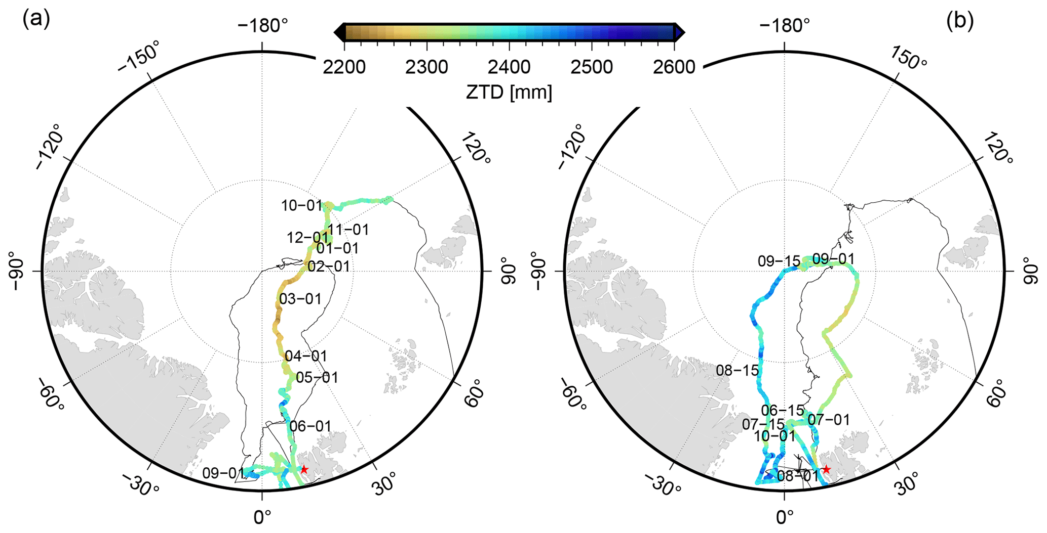
Figure 6Ship track with hourly ZTD values (color coded according to the ZTD); panel (a) shows the ZTD series for August 2019 to 5 June 2020, panel (b) shows the ZTDs for 6 June to 3 October 2019; selected time stamps are added; the red star marks Ny-Ålesund.
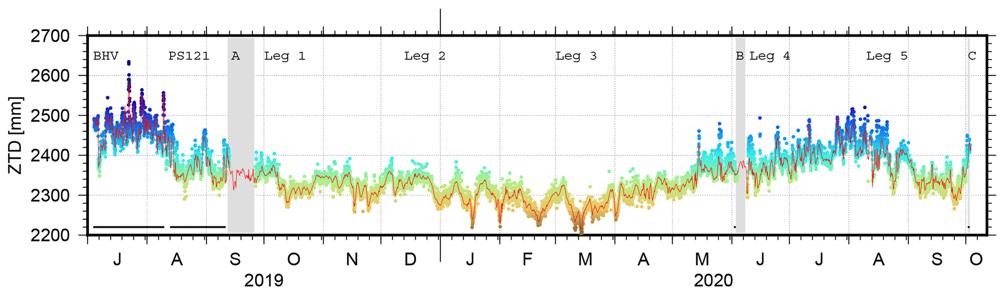
Figure 7ZTD time series: hourly ZTD values (color coded according to the ZTD, same scale as in Fig. 6) and 3-hourly ERA5-based ZTDs (red line); the cruise parts are indicated by labels, restricted time periods are shaded in gray; horizontal black lines indicate periods for which comparisons with terrestrial GNSS stations were possible.
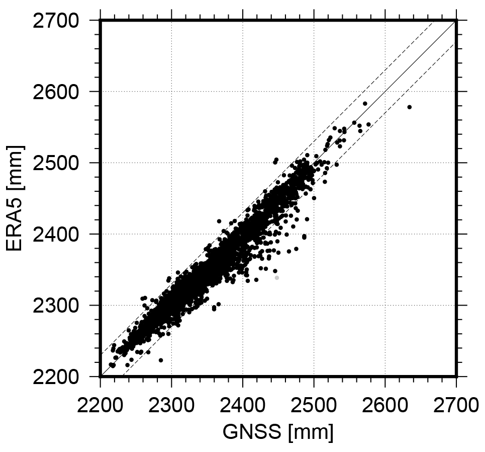
Figure 8 shows the direct comparison between the GNSS and the ERA5-based ZTD values. The correlation coefficient between both time series reaches 0.97, which agrees very well with the 97.2 % correlation presented in Wang et al. (2019). Interestingly, epochs where GNSS-based ZTDs are larger than the ERA5-based value occurred predominantly during the summer months in 2019 and 2020.
5.2 Comparison to onshore GNSS
The assessment of ZTDs determined for the GNSS receiver aboard RV Polarstern with respect to ZTDs derived for onshore GNSS receivers allows a second comparison option. A comparison between ship-based ZTD and land-based GNSS products is in general possible for (1) harbor stays with a close-by GNSS station and (2) periods where the ship's distance to a terrestrial reference station does not exceed a few hundred kilometers under stable weather conditions. The first comparison approach can be applied for the shipyard stay in Bremerhaven (6 weeks). Unfortunately, the harbor stay at Tromsø (1 week) could not be used for a comparison due to the data restrictions. The second approach is challenging given the remote character of the MOSAiC expedition. However, during PS121, the re-supply trip at Svalbard and RV Polarstern's return trip, the distance between the GNSS tracking stations at Ny-Ålesund, Svalbard and RV Polarstern was shorter than 200 km for several days. The distance limit of 200 km was chosen following the conclusions given in Wang et al. (2019). The related ZTDs are thus compared to the onshore GNSS at Ny-Ålesund. Reference ZTDs have been estimated within an operational GNSS processing system for meteorological applications, which is based on the GFZ Earth Parameter and Orbit determination System (EPOS.P8) software (Gendt et al., 2004; Wickert et al., 2020).
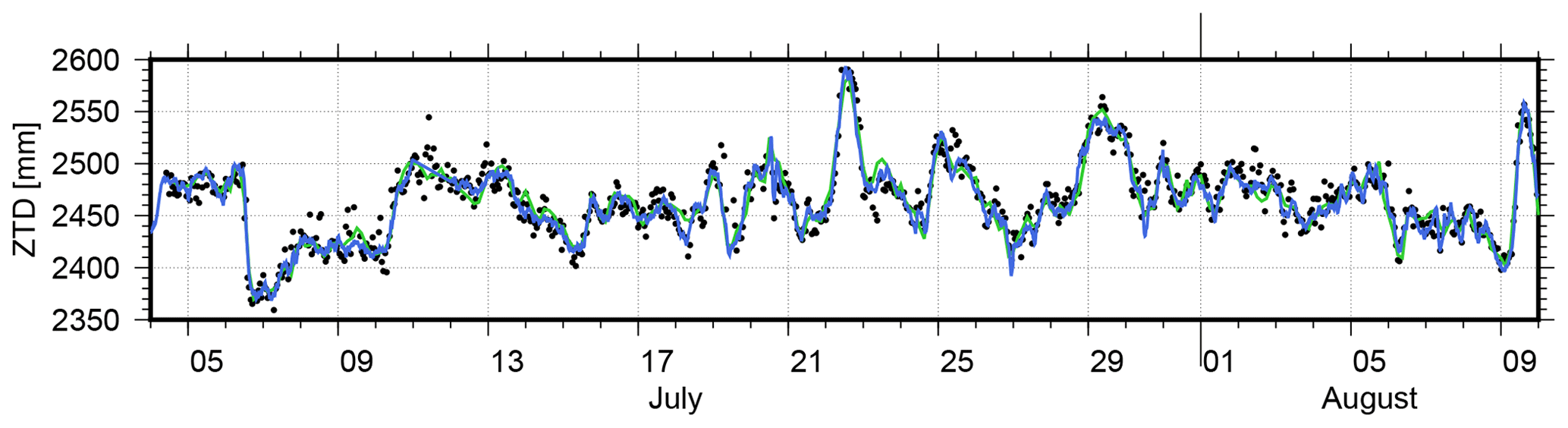
Figure 9ZTD time series during the shipyard stay in July and August 2019: hourly ZTD values from RV Polarstern (black dots) and SAPOS station 0994 (blue), as well as ERA5-based ZTDs (green).
For the shipyard stay in Bremerhaven, a reasonable mean difference of 1.5 ± 0.4 mm and an rms of 9.9 mm were estimated between ZTDs for RV Polarstern and German SAPOS station 0994. This station is located approximately 2.6 km from RV Polarstern and around 20 m above the ground like the GNSS antenna height at RV Polarstern. Therefore, no height correction was applied. Figure 9 shows the time series of derived ZTDs during the harbor and shipyard stay in Bremerhaven, including corresponding ZTD estimates for SAPOS station 0994 and the ERA5-based ZTD time series as an additional reference. Overall, a good agreement can be noted between the three ZTD solutions, while the sparser sampling of the ERA5 ZTD solution is visible (i.e., 3 h sampling for ERA5 compared to 1 h for GNSS). During this time, an rms of 12.0 mm and an average of 0.4 ± 0.7 mm are observed for the differences to the ERA5-based ZTDs. More details are provided in Table 3.
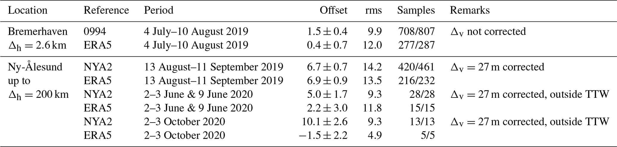
Table 3Summary of differences with respect to GNSS and ERA5 (always computed as the difference of RV Polarstern and the reference); Δh horizontal distance, Δv vertical difference; number of used/all samples is given; TTW indicates territorial waters; units: mm.
For Tromsø, only an indirect comparison between the ERA5-based ZTD time series and the permanent GNSS station TRO1 is possible. TRO1 is a GNSS station provided via the International GNSS Service (IGS, Johnston et al., 2017) and is located approximately 3 km from RV Polarstern's mooring and around 107 m above sea level. Consequently, these ZTDs were corrected for a height differences of 85 m using a rough delay correction of 0.3 mm m−1 for the hydrostatic part. A difference of 1.0 ± 0.8 mm and an rms of 6.1 mm reveal a good agreement for this comparison between GNSS and ERA5.

Figure 10Hourly ZTD values (black) compared to ZTDs derived for IGS station NYA2 (Ny-Ålesund, Svalbard, blue) during August/September 2019 (a), June 2020 (b) and October 2020 (c), and to ZTDs derived from ERA5 (green) and VLBI stations NYALES20 and NYALE13S (orange); the distance between RV Polarstern and NYA2 is represented in red.
The comparison between the ZTDs derived for RV Polarstern and the GNSS station in Ny-Ålesund, Svalbard, is more challenging due to the larger distances, the ship's speed and partly the performed ship operations. In addition, also the orographic setting might be a source for differences between the RV Polarstern measurements on open water and the measurements at the edge of a fjord surrounded by mountains in Ny-Ålesund. The reference station (NYA2) is a GNSS station operated by GFZ (Ramatschi et al., 2019) and observations and metadata are available within the IGS. Figure 10 shows Polarstern's ZTD series and the ERA5-based ZTD values. In addition, the geometrical distance between RV Polarstern and NYA2 is indicated by the red line. Whereas the observed good agreement between the on-board estimates and ERA5 is expected, the differences regarding NYA2 are partly larger. Especially during the PS121 expedition (Fram Strait), time shifts between the ZTD series can be observed for some periods, e.g., for 26–28 August. For these particular dates, the PS121 expedition report mentions a storm field close to Iceland affecting RV Polarstern with speeds of about 8 Bft (Beaufort units) (Metfies, 2020). During the re-supply stay in June 2020, ZTDs are not permitted. However, less accurate ZTDs are expected for this period considering the drop in the processed phase observations (see Fig. 3) potentially caused by the logistic activities. For the arrival and departure periods, the agreement is within the expected range. For the third interval, again, a good agreement is visible for 2 and 3 October 2020 but larger differences for the approaching period on 1 October 2020. While RV Polarstern approached Ny-Ålesund closely with distances to NYA2 below 2 km, the corresponding values are, however, restricted by the research agreement and cannot be used for the comparison. The statistics are summarized in Table 3. Overall, offsets and rms are below 10 and 14 mm, respectively. Compared to Wang et al. (2019) and Bosser et al. (2021), larger variations are derived for RV Polarstern most probably caused by the suboptimal antenna position.
5.3 Comparison to VLBI
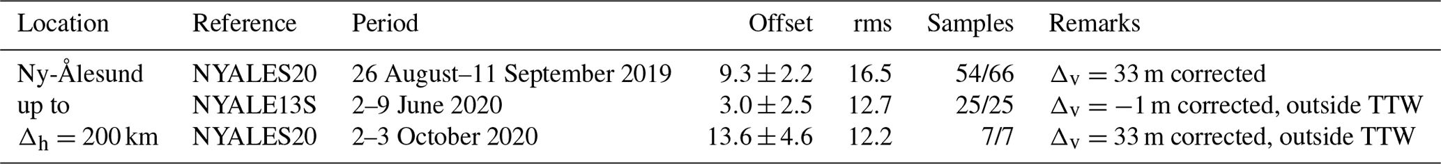
The geodetic fundamental site in Ny-Ålesund also allows a comparison between the ZTDs determined for the GNSS antenna aboard RV Polarstern and the ZTD observed by VLBI at the radio telescopes NYALES20 and NYALE13S2 for a completely external validation. Very long baseline interferometry is an interferometric technique measuring the time delay between the reception of signals transmitted by extragalactic radio sources at two or more antennas (Schuh and Behrend, 2012). Currently, VLBI sessions with global networks are not performed continuously but scheduled in twice-weekly 24 h sessions and provided within the International VLBI Service for Geodesy and Astrometry (IVS, Nothnagel et al., 2017). The high accuracy of VLBI-based troposphere estimates has been reported, for example, by Heinkelmann et al. (2007) and Balidakis et al. (2018). In the time span of 11 August to 12 September 2019, in total, nine 24 h sessions with NYALES20, during 20 May and 15 June 2020 seven sessions with NYALES20 or NYALE13S, and during 20 September and 4 October 2020 another five sessions with NYALES20 were analyzed using PORT (Potsdam Open Source Radio Interferometry Tool). PORT is GFZ's VLBI analysis software and is based on VieVS (Vienna VLBI Software, Böhm et al., 2012; Nilsson et al., 2015). The derived VLBI-based ZTDs are shown in orange in Fig. 10. First of all, it can be noted that the ZTDs of GNSS (NYA2) and VLBI agree well, which is expected due to the short horizontal distances between the stations3 and the highly accurate space techniques GNSS and VLBI. Overall, a good agreement is visible also between the VLBI and the RV Polarstern ZTDs. However, a few VLBI-based ZTDs differ significantly in August 2019, while also the GNSS ZTDs showed some larger differences for these days as reported above. For both June and October 2020, there were VLBI sessions while RV Polarstern was close to Svalbard. However, during these periods, RV Polarstern was mainly within the territorial waters around Svalbard in which ZTDs are restricted. In June, one session with NYALES20 is within the restricted period, while a comparison is allowed for a session with NYALE13S. For this session, an offset of 3.0 mm and an rms of 12.7 mm is determined over 25 ZTD differences. For October, a comparison is possible as well, however, only for a short period of 7 h. Similar to the comparison against onshore GNSS, offsets and rms values are below 16 mm. The statistical values are summarized in Table 4.
Table 4Summary of differences with respect to VLBI (always computed as the difference of RV Polarstern and the reference); number of used/all samples is given; units: mm.
This section discusses integrated water vapor values derived from the ZTD aboard RV Polarstern. The conversion between ZTD and IWV was performed by applying Eq. (2) of Bevis et al. (1994). The zenith wet delay was computed by subtracting the hydrostatic delay provided by ERA5 from the estimated ZTD values. The weighted mean temperature of the atmosphere Tm was calculated from the ERA5 data using Eq. (A18) of Davis et al. (1985). To derive hourly IWV, the 3-hourly ERA5 data are linearly interpolated.
Aboard RV Polarstern, Vaisala RS41 radiosondes were launched every 6 h during the entire MOSAiC expedition and moreover every 3 h for periods of specific interest. Based on the relative humidity data in the preliminary radiosonde dataset (Maturilli et al., 2021), vertically resolved specific humidity profiles were calculated by applying Hyland and Wexler (1983) and integrated over the atmospheric column to retrieve IWV. Measurements for which the radiosondes did not reach a height of at least 10 000 m are excluded in the following (0.9 %).
Figure 11 shows the comparison between the GNSS-based IWV and the radiosonde observations. Overall, an agreement of 0.08 ± 0.04 kg m−2 with an rms of 1.47 kg m−2 can be found together with a correlation coefficient of 0.97 between both datasets. In this comparison, 2.6 % of the overall 1495 difference, i.e., those values exceeding 5 kg m−2, are excluded. Comparable values are reported by Shoji et al. (2017) for a comparison between radiosonde-based PWV and GNSS in the northern Pacific. Bosser et al. (2021) reported slightly larger IWV biases with respect to ERA5 but similar variations with 2.2 and 2.7 kg m−2 for RV Atalante and RV Meteor, respectively. The majority of the absolute IWV values is below 5 kg m−2, as visible in Fig. 11. This result could be expected as, driven by the low air temperatures, the amount of atmospheric water vapor was very low during large parts of the transpolar drift. Consequently, IWV values observed by GNSS and radiosondes are below 5 kg m−2 from mid-October 2019 to the end of April 2020 with only a few exceptions. One example of such rapid moisture increase occurred in April 2020 and was associated with two warm-air intrusion events on 16 and 19 April. According to Magnusson et al. (2020), the warm air was pushed to the northeast in front of a low-pressure trough over Scandinavia in the first event. In contrast, the second event was driven by warm air transported northward on the western side of a high-pressure ridge that developed over Scandinavia. Both events on 16 and 19 April are well visible in the IWV time series shown in Fig. 12. For both events, the air temperature increased rapidly from around −20 to nearly 0 ∘C. Simultaneously, the IWV observed by GNSS increased from below 5 kg m−2 to 8 and 13 kg m−2 for the two events. For both events, a nearly perfect agreement between GNSS-derived and radiosonde-based IWVs is visible.
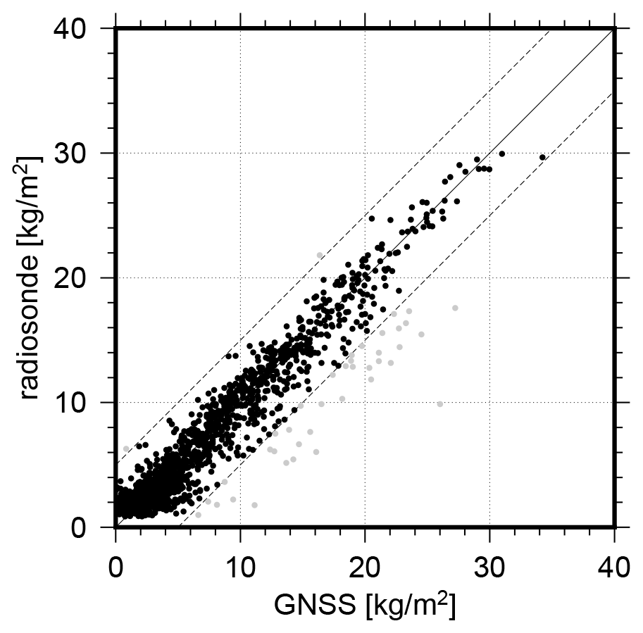
Figure 11Comparison of IWV derived from GNSS and radiosondes; differences > 5 kg m−2 are shown in gray (2.6 % of in total 1495 differences).
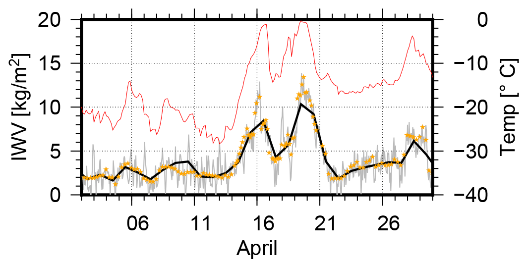
Figure 12GNSS-based IWV: hourly values (gray) and daily averaged (black); radiosonde-based IWV (orange stars); air temperature from ERA5 (red).
The MOSAiC expedition offered a unique opportunity to study polar environmental conditions during one full annual cycle. Besides other techniques, an on-board GNSS receiver allowed to monitor the variations of atmospheric water vapor above RV Polarstern. Based on 15 months of continuously tracked GNSS data, a kinematic PPP approach including GPS, GLONASS and Galileo was used to determine epoch-wise coordinates and hourly zenith total delays. By assessing the GNSS data, a reliable number of observations was found; however, it was disturbed by multipath effects due to suboptimal antenna location. With a few exceptions, the kinematic coordinates are well determined over the entire time span. For the static shipyard stay, the variations of the kinematic coordinates were within 5 cm for the horizontal and within 10 cm for the vertical component. The comparison of the GNSS-based ZTDs against ZTD derived from the ERA5 model shows a good agreement with an offset of 1.1 ± 0.2 mm and an rms of 10.2 mm over the entire period and a strong correlation of 0.97. Due to the remote character of the MOSAiC expedition, the comparison to terrestrial GNSS receivers was more challenging. For the harbor stay in Bremerhaven, we derived an offset of 1.5 ± 0.4 mm and a variation of around 1 cm. Comparing ZTDs up to 200 km against IGS station NYA2, larger biases of up to 10 mm and standard deviations up to 14 mm were noted and confirmed by comparing to ZTDs measured at the VLBI radio telescopes in Ny-Ålesund. Thanks to frequent radiosonde measurements during the MOSAiC expedition, a detailed comparison between GNSS-based IWV and radiosonde measurements was possible. The overall difference of 0.08 ± 0.04 kg m−2 and the rms of 1.47 kg m−2 show a good agreement of both techniques, which is also visible during two warm-air intrusions in April 2020. Overall, GNSS receivers aboard ships allow a cost-efficient and continuous monitoring of atmospheric water vapor over the oceans.
GNSS RINEX data and derived ZTD and IWV values are available at https://doi.org/10.5880/GFZ.1.1.2021.003 (Männel et al., 2021) and https://doi.org/10.5880/GFZ.1.1.2021.004 (Männel and Zus, 2021), respectively.
BM, FZ and GD defined the study with support from MS and JW, the PI of the GNSS experiment from GFZ during MOSAiC. BM, FZ, SG and KB processed the GNSS, ERA5 and VLBI data; MM and SD provided the radiosonde data. All authors contributed to the analysis, interpretation and discussion of the results. BM prepared the manuscript with major contributions from FZ, SG, HS and MM. All authors read and approved the final manuscript.
The authors declare that they have no conflict of interest.
Publisher's note: Copernicus Publications remains neutral with regard to jurisdictional claims in published maps and institutional affiliations.
The authors want to thank IGS, IVS, CODE and ECMWF for making the used data and products publicly available. We would also like to thank Thomas Gerber, Sylvia Magnussen, Markus Bradke and the technical staff of RV Polarstern for all support during GNSS installation, operations and data retrieval. Radiosonde data were obtained through a partnership between the leading Alfred Wegener Institute (AWI), the Atmospheric Radiation Measurement (ARM) User Facility, a US Department of Energy facility managed by the Biological and Environmental Research Program and the German Weather Service (DWD). Data used in this paper were produced as part of RV Polarstern cruise AWI_PS121 and of the international Multidisciplinary drifting Observatory for the Study of the Arctic Climate (MOSAiC) with the tag MOSAiC20192020 (AWI_PS122_00). Finally, we thank the anonymous reviewers for their assistance in evaluating this paper and their helpful recommendations.
The article processing charges for this open-access publication were covered by the Helmholtz Centre Potsdam – GFZ German Research Centre for Geosciences.
This paper was edited by Roeland Van Malderen and reviewed by two anonymous referees.
Alfred Wegener Institute: Polar Research and Supply Vessel POLARSTERN Operated by the Alfred-Wegener-Institute, JLSRF, 3, A119, https://doi.org/10.17815/jlsrf-3-163, 2017. a
Alshawaf, F., Zus, F., Balidakis, K., Deng, Z., Hoseini, M., Dick, G., and Wickert, J.: On the Statistical Significance of Climatic Trends Estimated From GPS Tropospheric Time Series, J. Geophys. Res., 123, 10967–10990, https://doi.org/10.1029/2018JD028703, 2018. a
Balidakis, K., Nilsson, T., Zus, F., Glaser, S., Heinkelmann, R., Deng, Z., and Schuh, H.: Estimating Integrated Water Vapor Trends From VLBI, GPS, and Numerical Weather Models: Sensitivity to Tropospheric Parameterization, J. Geophys. Res.-Atmos., 123, 6356–6372, https://doi.org/10.1029/2017JD028049, 2018. a
Bevis, M., Businger, S., Chiswell, S., Herring, T. A., Anthes, R. A., Rocken, C., and Ware, R. H.: GPS Meteorology: Mapping Zenith Wet Delays onto Precipitable Water, J. Appl. Meteorol. Climatol., 33, 379–386, https://doi.org/10.1175/1520-0450(1994)033<0379:GMMZWD>2.0.CO;2, 1994. a
Böhm, J., Werl, B., and Schuh, H.: Troposphere mapping functions for GPS and VLBI from European Centre for medium-range weather forecasts operational analysis data, J. Geophys. Res., 111, B02406, https://doi.org/10.1029/2005JB003629, 2006. a
Böhm, J., Böhm, S., Nilsson, T., Pany, A., Plank, L., Spicakova, H., Teke, K., and Schuh, H.: The New Vienna VLBI Software VieVS, in: Geodesy for Planet Earth, edited by: Kenyon, S., Pacino, M. C., and Marti, U., vol. 136 of International Association of Geodesy Symposia, Springer Berlin Heidelberg, 1007–1011, https://doi.org/10.1007/978-3-642-20338-1_126, 2012. a
Boniface, K., Champollion, C., Chery, J., Ducrocq, V., Rocken, C., Doerflinger, E., and Collard, P.: Potential of shipborne GPS atmospheric delay data for prediction of Mediterranean intense weather events, Atmos. Sci. Lett., 13, 250–256, https://doi.org/10.1002/asl.391, 2012. a
Bosser, P., Bock, O., Flamant, C., Bony, S., and Speich, S.: Integrated water vapour content retrievals from ship-borne GNSS receivers during EUREC4A, Earth Syst. Sci. Data, 13, 1499–1517, https://doi.org/10.5194/essd-13-1499-2021, 2021. a, b, c, d
Dach, R., Lutz, S., Walser, P., and Fridez, P.: Bernese GNSS Software Version 5.2, Bern, https://doi.org/10.7892/boris.72297, 2015. a
Davis, J. L., Herring, T. A., Shapiro, I. I., Rogers, A. E. E., and Elgered, G.: Geodesy by radio interferometry: Effects of atmospheric modeling errors on estimates of baseline length, Radio Sci., 20, 1593–1607, https://doi.org/10.1029/RS020i006p01593, 1985. a
Elgered, G. and Wickert, J.: Monitoring of the Neutral Atmosphere, Springer International Publishing, 1109–1138, https://doi.org/10.1007/978-3-319-42928-1_38, 2017. a
Estey, L. and Meertens, C.: TEQC: The Multi-Purpose Toolkit for GPS/GLONASS Data, GPS Solut., 3, 42–49, https://doi.org/10.1007/PL00012778, 1999. a
Fujita, M., Kimura, F., Yoneyama, K., and Yoshizaki, M.: Verification of precipitable water vapor estimated from shipborne GPS measurements, Geophys. Res. Lett., 35, L13803, https://doi.org/10.1029/2008GL033764, 2008. a
Gendt, G., Dick, G., Reigber, C., Tomassini, M., Liu, M., and Ramatschi, M.: Near Real Time GPS Water Vapor Monitoring for Numerical Weather Prediction in Germany, J. Met. Soc, 82, 361–370, https://doi.org/10.2151/jmsj.2004.361, 2004. a, b, c
Guerova, G., Jones, J., Douša, J., Dick, G., de Haan, S., Pottiaux, E., Bock, O., Pacione, R., Elgered, G., Vedel, H., and Bender, M.: Review of the state of the art and future prospects of the ground-based GNSS meteorology in Europe, Atmos. Meas. Tech., 9, 5385–5406, https://doi.org/10.5194/amt-9-5385-2016, 2016. a
Heinkelmann, R., Böhm, J., Schuh, H., Bolotin, S., Engelhardt, G., MacMillan, D. S., Negusini, M., Skurikhina, E., Tesmer, V., and Titov, O.: Combination of long time-series of troposphere zenith delays observed by VLBI, J. Geod., 81, 483–501, https://doi.org/10.1007/s00190-007-0147-z, 2007. a
Hersbach, H., Bell, B., Berrisford, P., Hirahara, S., Horányi, A., Muñoz Sabater, J., Nicolas, J., Peubey, C., Radu, R., Schepers, D., Simmons, A., Soci, C., Abdalla, S., Abellan, X., Balsamo, G., Bechtold, P., Biavati, G., Bidlot, J., Bonavita, M., De Chiara, G., Dahlgren, P., Dee, D., Diamantakis, M., Dragani, R., Flemming, J., Forbes, R., Fuentes, M., Geer, A., Haimberger, L., Healy, S., Hogan, R. J., Hólm, E., Janisková, M., Keeley, S., Laloyaux, P., Lopez, P., Lupu, C., Radnoti, G., de Rosnay, P., Rozum, I., Vamborg, F., Villaume, S., and Thépaut, J.-N.: The ERA5 global reanalysis, Q. J. R. Meteorol. Soc., 146, 1999–2049, https://doi.org/10.1002/qj.3803, 2020. a
Hyland, R. W. and Wexler, A.: Formulations for the Thermodynamic Properties of the saturated Phases of H2O from 173.15 K to 473.15 K, ASHRAE Trans, 89, 500–519, 1983. a
Johnston, G., Riddell, A., and Hausler, G.: The International GNSS Service, Springer International Publishing, Cham, Switzerland, 967–982, https://doi.org/10.1007/978-3-319-42928-1, 2017. a
Kiehl, J. T. and Trenberth, K. E.: Earth's Annual Global Mean Energy Budget, Bull. Amer. Meteor., 78, 197–208, https://doi.org/10.1175/1520-0477(1997)078<0197:EAGMEB>2.0.CO;2, 1997. a
Magnusson, L., Day, J., Sandu, I., and Svensson, G.: Warm intrusions into the Arctic in April 2020, ECMWF newsletter, available at: https://www.ecmwf.int/en/newsletter/164/news/warm-intrusions-arctic-april-2020 (last access: 21 July 2021), 2020. a
Männel, B. and Zus, F.: GNSS-based zenith total delays observed during the MOSAiC Campaign 2019–2020, GFZ Data Services [data set], https://doi.org/10.5880/GFZ.1.1.2021.004, 2021. a
Männel, B., Bradke, M., Semmling, M., Wickert, J., Gerber, T., Magnussen, S., Spreen, G., Ricker, R., Kaleschke, L., and Tavri, A.: Geodetic GNSS data for atmospheric sounding recorded during the MOSAiC Expedition 2019–2020, GFZ Data Services [data set], https://doi.org/10.5880/GFZ.1.1.2021.003, 2021. a
Maturilli, M., Holdridge, D. J., Dahlke, S., Graeser, J., Sommerfeld, A., Jaiser, R., Deckelmann, H., and Schulz, A.: Initial radiosonde data from 2019-10 to 2020-09 during project MOSAiC, PANGAEA, https://doi.org/10.1594/PANGAEA.928656, 2021. a
Metfies, K.: The Expedition PS121 of the Research Vessel POLARSTERN to the Fram Strait in 2019, Reports on Polar and Marine Research, https://doi.org/10.2312/BzPM_0738_2020, 2020. a
Nilsson, T., Soja, B., Karbon, M., Heinkelmann, R., and Schuh, H.: Application of Kalman filtering in VLBI data analysis, Earth Planets Space, 67, 136, https://doi.org/10.1186/s40623-015-0307-y, 2015. a
Ning, T., Wang, J., Elgered, G., Dick, G., Wickert, J., Bradke, M., Sommer, M., Querel, R., and Smale, D.: The uncertainty of the atmospheric integrated water vapour estimated from GNSS observations, Atmos. Meas. Tech., 9, 79–92, https://doi.org/10.5194/amt-9-79-2016, 2016. a
Nischan, T.: GFZRNX – RINEX GNSS Data Conversion and Manipulation Toolbox, GFZ Data Services, https://doi.org/10.5880/GFZ.1.1.2016.002, 2016. a
Nothnagel, A., Artz, T., Behrend, D., and Malkin, Z.: International VLBI Service for Geodesy and Astrometry – Delivering high-quality products and embarking on observations of the next generation, J. Geod., 91, 711–712, https://doi.org/10.1007/s00190-016-0950-5, 2017. a
Prange, L., Villiger, A., Sidorov, D., Schaer, S., Beutler, G., Dach, R., and Jäggi, A.: Overview of CODEs MGEX solution with the focus on Galileo, Adv. Space Res., 66, 2786–2798, https://doi.org/10.1016/j.asr.2020.04.038, 2020. a
Ramatschi, M., Bradke, M., Nischan, T., and Männel, B.: GNSS data of the global GFZ tracking network, V.1, GFZ Data Services, https://doi.org/10.5880/GFZ.1.1.2020.001, 2019. a
Rebischung, P. and Schmid, R.: IGS14/igs14.atx: a new framework for the IGS products, in: AGU Fall Meeting, 12–16 December 2016, San Francisco, CA, USA, available at: https://mediatum.ub.tum.de/doc/1341338/le.pdf (last access: 21 July 2021), 2016. a
Rinke, A., Segger, B., Crewell, S., Maturilli, M., Naakka, T., Nygard, T., Vihma, T., Alshawaf, F., Dick, G., Wickert, J., and Keller, J.: Trends of Vertically Integrated Water Vapor over the Arctic during 1979–2016, J Climate, 32, 6097–6116, https://doi.org/10.1175/JCLI-D-19-0092.1, 2019. a
Rocken, C., Johnson, J., Van Hove, T., and Iwabuchi, T.: Atmospheric water vapor and geoid measurements in the open ocean with GPS, Geophys. Res. Lett., 32, L12813, https://doi.org/10.1029/2005GL022573, 2005. a
Schuh, H. and Behrend, D.: VLBI: A fascinating technique for geodesy and astrometry, J. Geodyn., 61, 68–80, https://doi.org/10.1016/j.jog.2012.07.007, 2012. a
Semmling, M., Wickert, J., Kress, F., Hoque, M. M., Divine, D., and Gerland, S.: Sea-ice permittivity derived from GNSS reflection profiles: Results of the MOSAiC expedition, IEEE TGRS, in review, 2021. a
Shangguan, M., Heise, S., Bender, M., Dick, G., Ramatschi, M., and Wickert, J.: Validation of GPS atmospheric water vapor with WVR data in satellite tracking mode, Ann. Geophys., 33, 55–61, https://doi.org/10.5194/angeo-33-55-2015, 2015. a
Shoji, Y., Sato, K., and Yabuki, M.: Comparison of shipborne GNSS-derived precipitable water vapor with radiosonde in the western North Pacific and in the seas adjacent to Japan, Earth Planets Space, 69, 153, https://doi.org/10.1186/s40623-017-0740-1, 2017. a, b
Steinke, S., Eikenberg, S., Löhnert, U., Dick, G., Klocke, D., Di Girolamo, P., and Crewell, S.: Assessment of small-scale integrated water vapour variability during HOPE, Atmos. Chem. Phys., 15, 2675–2692, https://doi.org/10.5194/acp-15-2675-2015, 2015. a
Wang, J., Wu, Z., Semmling, M., Zus, F., Gerland, S., Ramatschi, M., Ge, M., Wickert, J., and Schuh, H.: Retrieving Precipitable Water Vapor From Shipborne Multi-GNSS Observations, Geophys. Res. Lett., 46, 5000–5008, https://doi.org/10.1029/2019GL082136, 2019. a, b, c, d, e
Wickert, J., Dick, G., Schmidt, T., Asgarimehr, M., Antonoglou, N., Arras, C., Brack, A., Ge, M., Kepkar, A., Männel, B., Nguyen Thai, C., Oluwadare, T. S., Schuh, H., Semmling, M., Simeonov, T., Vey, S., Wilgan, K., and Zus, F.: GNSS Remote Sensing at GFZ: Overview and Recent Results, ZfV: Zeitschrift für Geodäsie, Geoinformation und Landmanagement, 145, 266–278, https://doi.org/10.12902/zfv-0320-2020, 2020. a
Woods, C. and Caballero, R.: The role of moist intrusions in winter Arctic warming and sea ice declin, J. Climate, 29, 4473–4485, https://doi.org/10.1175/JCLI-D-15-0773.1, 2016. a
Zumberge, J. F., Heflin, M. B., Jefferson, D. C., Watkins, M. M., and Webb, F. H.: Precise Point Positioning for the efficient and robust analysis of GPS data from large networks, J. Geophys. Res., 102, 5005–5018, https://doi.org/10.1029/96JB03860, 1997. a
Zus, F., Bender, M., Deng, Z., Dick, G., Heise, S., Shangguan, M., and Wickert, J.: A methodology to compute GPS slant total delays in a numerical weather model, Radio Sci., 47, RS2018, https://doi.org/10.1029/2011RS004853, 2012. a
Tide gauge data are taken from http://159.162.103.47/en/sehavniva/Lokasjonsside/?cityid=9000020&city=Troms%C3%B8 (last access: 21 July 2021).
active since 8 January 2020.
273 m for NYA2–NYALES20 and 1539 m for NYA2–NYALE13S.
- Abstract
- Introduction
- GNSS installation and data availability
- Processing strategy
- Assessment of kinematic coordinates
- Assessment of zenith total delay
- Assessment of integrated water vapor
- Conclusions
- Data availability
- Author contributions
- Competing interests
- Disclaimer
- Acknowledgements
- Financial support
- Review statement
- References