the Creative Commons Attribution 4.0 License.
the Creative Commons Attribution 4.0 License.
 | 06 Aug 2021
Physical characteristics of frozen hydrometeors inferred with parameter estimation
Frozen hydrometeors are found in a huge range of shapes and sizes, with variability on much smaller scales than those of typical model grid boxes or satellite fields of view. Neither models nor in situ measurements can fully describe this variability, so assumptions have to be made in applications including atmospheric modelling and radiative transfer. In this work, parameter estimation has been used to optimise six different assumptions relevant to frozen hydrometeors in passive microwave radiative transfer. This covers cloud overlap, convective water content and particle size distribution (PSD), the shapes of large-scale snow and convective snow, and an initial exploration of the ice cloud representation (particle shape and PSD combined). These parameters were simultaneously adjusted to find the best fit between simulations from the European Centre for Medium-range Weather Forecasts (ECMWF) assimilation system and near-global microwave observations covering the frequency range 19 to 190 GHz. The choices for the cloud overlap and the convective particle shape were particularly well constrained (or identifiable), and there was even constraint on the cloud ice PSD. The practical output is a set of improved assumptions to be used in version 13.0 of the Radiative Transfer for TOVS microwave scattering package (RTTOV-SCATT), taking into account newly available particle shapes such as aggregates and hail, as well as additional PSD options. The parameter estimation explored the full parameter space using an efficient assumption of linearly additive perturbations. This helped illustrate issues such as multiple minima in the cost function, and non-Gaussian errors, that would make it hard to implement the same approach in a standard data assimilation system for weather forecasting. Nevertheless, as modelling systems grow more complex, parameter estimation is likely to be a necessary part of the development process.
- Article
(9702 KB) - Full-text XML
- BibTeX
- EndNote


Clouds and precipitation are some of the most uncertain processes in the earth system, leading to systematic errors in models (e.g. Klein et al., 2009; Forbes et al., 2016) and big uncertainties in climate change predictions (e.g. Zelinka et al., 2020). The parametrisations that represent hydrometeors1 in global models rely on physically informed heuristic abstractions, such as the representation of convection by upward and downward mass fluxes (e.g. Tiedtke, 1989). They also rely on compressing reality into simple functional fits, such as particle fall-speed and size distributions (e.g. Locatelli and Hobbs, 1974; Field et al., 2007; Heymsfield et al., 2013) or cloud overlap models (e.g. Hogan and Illingworth, 2000). Typically these parametrisations are informed by observations, but they also require tuning of uncertain and unconstrained parameters and are dependent on expert knowledge and trial and error. Although progress continues with improved models and reduced systematic errors (e.g. Bechtold et al., 2014; Forbes et al., 2011), there remain many uncertainties and compensating errors, and increasing complexity can bring additional problems of parameter tuning, making new developments ever harder. This motivates a more objective, automated, and observation-driven approach to developing parametrisations, using machine learning (ML), data assimilation (DA), or a mixture of both (e.g. Schneider et al., 2017; Rasp et al., 2018; Morrison et al., 2020; Geer, 2021). The process of learning model parameters using data assimilation is known as parameter estimation, with cloud and precipitation parameters a major target (e.g. Norris and Da Silva, 2007; Ruckstuhl and Janjić, 2020; Kotsuki et al., 2020).
Physical assumptions also need to be made in the forward models of satellite radiances that are required for making cloud and precipitation retrievals (e.g. Kummerow et al., 2001) or for assimilating such observations in weather forecasting (e.g. Geer et al., 2018). In particular, all-sky microwave observations are strongly sensitive to macrophysical and microphysical parameters of cloud and precipitation, most of which are not prognostic variables in forecast models. For example there is typically only a prognostic description of hydrometeor mixing ratio, and if the particle size distribution (PSD) and particle shape are constrained by assumed diagnostic relationships in the model, these may not give good results in the radiative transfer, due to the different physical sensitivities of each context. Further, such assumptions are not even necessarily consistent among the different components of one forecast model (Geer et al., 2017a). Hence, setting the physical assumptions used in the radiative transfer consistently with those of the forecast model is rarely done (e.g. Sieron et al., 2017) and remains a long-term aim. Instead, as with the development of forecast models, radiative transfer assumptions have often been set independently and by trial and error, expert knowledge (e.g. Di Michele et al., 2012), or by closure studies (e.g. Kulie et al., 2010; Ekelund et al., 2020). Similar to a closure study, a parameter search by Geer and Baordo (2014) found a snow particle shape by minimising the discrepancy between passive microwave observations and the equivalent radiances simulated from a forecast model. The current work builds on this by simultaneously estimating the values for six physical parameters relating to frozen hydrometeors and by using a more sophisticated estimation framework.
This work has dual motivations: one is to explore parameter estimation as a way of using observations to improve physical models; another is the more practical issue of updating the physical assumptions in the RTTOV model (Radiative Transfer for TOVS Saunders et al., 2018) and in particular its microwave/sub-millimetre scattering radiative transfer component, RTTOV-SCATT (Bauer et al., 2006). Since the earlier study (Geer and Baordo, 2014), a wider and more physical range of frozen particle representations has become available (e.g. Kneifel et al., 2018; Eriksson et al., 2018), and the observation operator offers additional PSD choices and a more flexible representation of hydrometeors (Geer et al., 2021). There is also a need to prepare for new satellite instruments operating at sub-millimetre (sub-mm) wavelengths, which will be more sensitive to the microphysical properties of cloud ice, particularly the Ice Cloud Imager (ICI, Buehler et al., 2007; Eriksson et al., 2020). The practical output of this work is therefore to provide the default physical configuration for RTTOV-SCATT in v13.0 of RTTOV, which was released in November 2020 (Saunders et al., 2020). Future iterations of this work will also seek to include the forecast model moist physics in the parameter estimation, but for the moment this is excluded.
The weather forecasting system being used is the Integrated Forecasting System (IFS, ECMWF, 2019) operated by the European Centre for Medium-range Weather Forecasts (ECMWF). This is described in Sect. 2.1, and the RTTOV-SCATT observation operator is covered in Sect. 2.2. The observations used in the parameter estimation come from the Special Sensor Microwave Imager/Sounder (SSMIS, Kunkee et al., 2008) and are described in Sect. 2.3. The six different microphysical and macrophysical parameters to be optimised are described in Sect. 3. Overall, Sects. 2 and 3 will be seen to contain a wealth of technical detail, but this is probably inescapable in a successful parameter estimation, which still relies on expert knowledge. The method for parameter estimation is a complete but efficient search of parameter space; this is described in Sect. 4. Section 5 describes the results of global and situation-dependent parameter searches and tests the robustness of the chosen parameter sets. Section 6 is a discussion: first, reviewing what has been learnt about physical parameters (Sect. 6.1); second, placing this work in the wider context of parameter estimation studies and Bayesian inverse methods (Sect. 6.2). The conclusion is Sect. 7.
2.1 Weather forecasting system
The core of this work is to compare model simulations to real observations, in other words model–observation closure. The tools for this are provided within the IFS. The data assimilation component provides high-quality initial conditions of the earth system (the analysis fields); a short run of the forecast model provides the “background” geophysical fields at the observation time and location, and the observation operator maps from model fields to the observations – here the radiances measured by satellites. The parameter estimation is done with passive monitoring experiments, which take their background fields from a fixed reference run of the DA system. Hence, the background geophysical fields are (with one exception) held constant while only the physical assumptions in the observation operator are varied.
Experiments were based around cycle 46r1 of the IFS (ECMWF, 2019), but adding a development version of RTTOV that is described in the next section. The experiments used a resolution of Tco399 or roughly 28 km horizontally2. There were 137 levels in the vertical, from the surface to 0.01 hPa. The data assimilation process used to create the fixed reference analyses used a 12 h cycling 4D-Var (Rabier et al., 2000) with three inner-loops at TL59/TL255/TL255 resolution3 corresponding to 125 and 78 km respectively. Despite having a slightly lower horizontal resolution compared to the operational version, this still provides high-quality background fields and is the standard configuration for testing at ECMWF. See Geer et al. (2017b) for a summary of all-sky microwave data usage in the assimilation system and Hersbach et al. (2020) for a broader overview of data usage in the IFS.
Cloud and precipitation in the IFS are generated using a set of physical parametrisations. Large-scale (stratiform) cloud and precipitation mixing ratios are prognostic variables that are subject to advection and whose interactions, sources, and sinks are governed by the Tiedtke (1993) parametrisation with subsequent improvements (e.g. Tompkins et al., 2007; Forbes and Tompkins, 2011). Large-scale cloud fraction is also a prognostic variable in this scheme. Moist convection is represented by a diagnostic mass-flux parametrisation (Tiedtke, 1989; Bechtold et al., 2014). The convective core hydrometeors are represented by the updraught and downdraught mass fluxes, which are assumed to occupy a fixed 5 % of the grid box. Cloud water and ice can be detrained into the large-scale scheme, allowing convection to form anvil cloud.
2.2 Observation operator
The observation operator for satellite radiances in the IFS is RTTOV (Saunders et al., 2018). Within this, RTTOV-SCATT (Bauer et al., 2006) provides the all-sky microwave capabilities. The all-sky radiance simulated by RTTOV-SCATT is the weighted combination of radiances from two independent column calculations: one that is completely clear, Iclear, and one with horizontally homogeneous cloud and precipitation, Icloud. The cloudy column is weighted by an effective cloud fraction C to approximate the nonlinear effect of sub-grid variability of cloud and precipitation, which is sometimes known as the beam-filling effect (e.g. Geer et al., 2009a; Barlakas and Eriksson, 2020). Hence the all-sky radiance is
This is then converted to black-body equivalent brightness temperature (TB, in K), which is the usual, more intuitive variable to represent satellite radiance observations. The effective cloud fraction C simplifies what could be a complex 3D arrangement of cloud and precipitation. Two options for deriving C will be tested in the parameter search (Sect. 3.1).
In Eq. (1) the clear column accounts only for the surface interaction and gaseous absorption. In the cloudy column, scattering radiative transfer is represented using the delta-Eddington approach (Joseph et al., 1976; Kummerow, 1993; Bauer et al., 2006). Although simple compared to more exact scattering methods, this is fast enough for use in a weather forecasting system and still accurate compared to reference models.
One simplification in the scattering radiative transfer is the treatment of polarisation. Each polarisation is considered independent, and hydrometeor optical properties are invariant with polarisation. This neglects the polarising effects of scattering from particles, which can transfer energy from one polarisation to another, and causes optical properties to vary as a function of polarisation and viewing angle. RTTOV v13.0 will have a simplified treatment of polarised scattering from preferentially oriented frozen hydrometeors; this reduces errors in the simulated vertical–horizontal polarisation difference by 10–15 K (Barlakas et al., 2021). This is not used in the main study; however, the parameter estimation is updated at the end, taking account of the new polarisation scheme, to provide a self-consistent final configuration for RTTOV v13.0 (Sect. 5.4).
The surface interaction is treated as specular reflection. Over ice-free ocean surfaces, this is handled by the FASTEM-6 surface emissivity model (Kazumori et al., 2016), which includes a simplified treatment for diffuse scattering. Over sea ice and over land, an all-sky dynamic emissivity retrieval operates at lower frequencies to supply the surface emissivity for the 50 and 183 GHz sounding channels (Baordo and Geer, 2016). The TELSEM surface emissivity database (Aires et al., 2011) is used for the other channels of SSMIS over land surfaces and also as a backup when the retrieval is not possible. In the passive monitoring experiments used here, a change to physical assumptions in the radiative transfer can affect the dynamic emissivity retrieval. In practice, the effect is negligible, and even in the convective graupel experiment (the biggest change tested; see Table 2) the maximum change in surface emissivity is tiny at around 1e−6.
The scattering solver requires the bulk optical properties of each layer of atmosphere. Hydrometeor optical properties (extinction, single-scattering albedo, and the asymmetry parameter) are supplied from lookup tables as a function of frequency, temperature, hydrometeor type, and hydrometeor water content. Changes to the microphysical assumptions explored in this work were made by changing these lookup tables, which are generated by an offline tool available within RTTOV (Geer et al., 2021). This integrates single-particle optical properties over the assumed particle size distribution, given the water content. It offers a choice of hydrometeor representations based on Mie spheres or non-spherical particles from the Liu (2008) and ARTS (Eriksson et al., 2018) databases. Version 13.0 includes new options for particle size distributions that were added in support of the current work. From the available options, four sets of parameters relating to large-scale snow, convective snow, and cloud ice were added to the parameter estimation as will be described in Sect. 3.
As discussed, the IFS has four large-scale prognostic hydrometeors, a prognostic cloud fraction, and a diagnostic large-scale precipitation fraction. Additionally, diagnostic mass fluxes for snow and rain represent convection, which is assumed to take 5 % of the grid box area. This is the complete set of cloud and precipitation information provided to RTTOV-SCATT, although some conversions are needed. To standardise the treatment with the convection fluxes, all six hydrometeors (rain, snow, cloud ice, and cloud water from the large-scale scheme; rain and snow from the convection scheme) are extracted from the model as fluxes (kg m−2 s−1) and then converted to mass mixing ratios (kg kg−1) before input to RTTOV-SCATT (see Geer et al., 2007, Appendix B). Strictly, this ratio is defined as the mass of the hydrometeor with respect the mass of moist air. However, due to the lack of a widely used terminology to specify whether hydrometeor mixing ratios are based on dry or moist air, this quantity is referred to throughout as just “mixing ratio”. The assumptions involved in obtaining the mixing ratio from the flux make the convective mixing ratio particularly uncertain (Geer et al., 2017a), but rather than adjust the assumptions in the model, here the parameter estimation is used to estimate a scaling factor to adjust the convective snow mixing ratio directly – further details in Sect. 3.
In the IFS, RTTOV-SCATT has been used in a four-hydrometeor configuration until now (rain, snow, cloud water, cloud ice) with the convective rain and snow mixing ratios added together with the large-scale rain and snow respectively; this provides the control setup. Going forward, the aim is a five-hydrometeor configuration, adding a new hydrometeor type specifically for convective snow, which is no longer combined with the large-scale snow. Within RTTOV-SCATT this hydrometeor is loosely referred to as “graupel”, but strictly it is for convective snow, making no assumptions on the particle habit. The most important causes of uncertainty in the radiative transfer are these microphysical assumptions, along with the representation of sub-grid heterogeneity (Bennartz and Greenwald, 2011; Barlakas and Eriksson, 2020) – hence the attempt to improve these aspects through parameter estimation.
2.3 Observations
This study uses observations from the Special Sensor Microwave Imager/Sounder (SSMIS, Kunkee et al., 2008). This is a conical-scanning microwave sensor, meaning that it has an approximately fixed zenith angle and polarisation across its swath. There are 24 channels on the instrument, of which 13 have been selected for use in this study (Table 1). Although SSMIS has additional calibration issues (e.g. Bell et al., 2008) compared to later microwave imagers such as the GPM microwave imager (GMI, Draper et al., 2015), these are mostly corrected by bias correction, which has been extensively used at ECMWF for all-sky assimilation and parameter estimation (Geer et al., 2017b; Geer and Baordo, 2014). The advantage of using SSMIS is that, with its temperature sounding channels around 50 GHz, it is a single instrument that covers the majority of frequencies currently in use or planned for use in all-sky assimilation (Geer et al., 2018), with the main exception being frequencies above 190 GHz, which will not be available from space until the launch of ICI in 2024. For the IFS, the observations are superobbed onto an 80 km by 80 km grid (Geer and Bauer, 2010) which averages together at least nine original SSMIS observations. This standardises the resolution across frequencies and helps match the effective resolution of cloud in the forecast model (note the simulations are made using the model grid point nearest to the centre of the superob).
Table 1SSMIS channels used in this study, ordered by frequency and polarisation.

Pol.: polarisation; v: vertical polarisation; h: horizontal polarisation; TCWV: total column water vapour; LT: lower troposphere; MT: mid-troposphere; UT: upper troposphere.
For the parameter estimation, SSMIS observations are taken from the F-17 satellite over a 10 d study period from 13–22 June 2019 inclusive. The selection of observations aims to include as much data as possible, even in situations where the observations are not well-enough represented to be used in active assimilation. The philosophy is that unless difficult situations are included as a constraint in the parameter estimation, the quality of radiative transfer in those situations will never become good enough to allow them to be used. This accepts the risk that unrelated systematic errors, such as poor surface emissivity, will lead to compensating biases in the parameter estimation.
Figure 1 illustrates the number of observations available in the study period, using a logarithmic colour scale. These are accumulated in the same 10∘ by 10∘ latitude–longitude bins that will be used in the cost function for the parameter estimation (Sect. 4). Observations are only excluded in areas of orography higher than 800 m, areas of sea ice, in mixed scenes where the grid point land–water mask is neither completely land or completely ocean, and over land where both the dynamic emissivity retrieval and the atlas backup failed. In any one bin, observations must be all ocean or all land, favouring the larger number. Typically around 3000 observations are available per bin over ice-free oceans and around 1000 observations over land areas; an approximate total of 1 million observations is used. The main losses are due to sea ice, the orography check, and the restriction on mixed scenes.
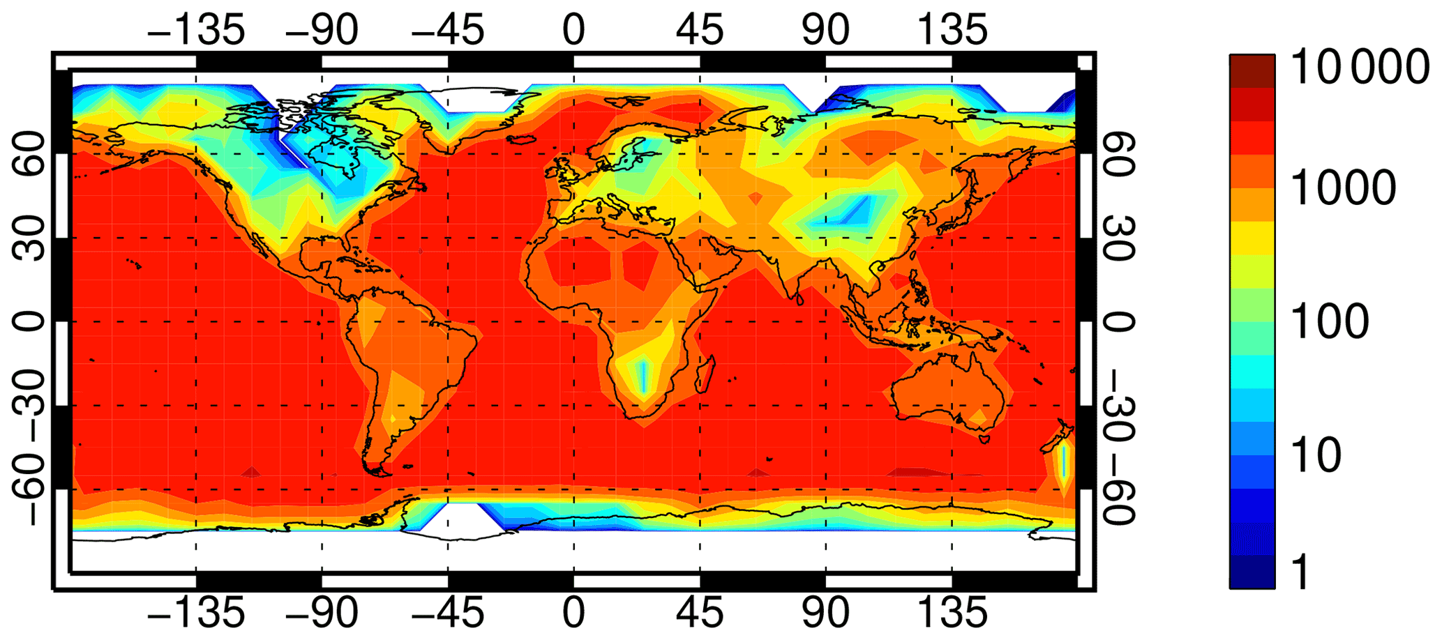
Figure 1Number of SSMIS F-17 observations (superobs) selected in the 13–22 June 2019 study period per 10∘ by 10∘ latitude–longitude bin. The colour scale is logarithmic to highlight data-poor areas. White areas have no observations. A total of 916 258 observations are included.
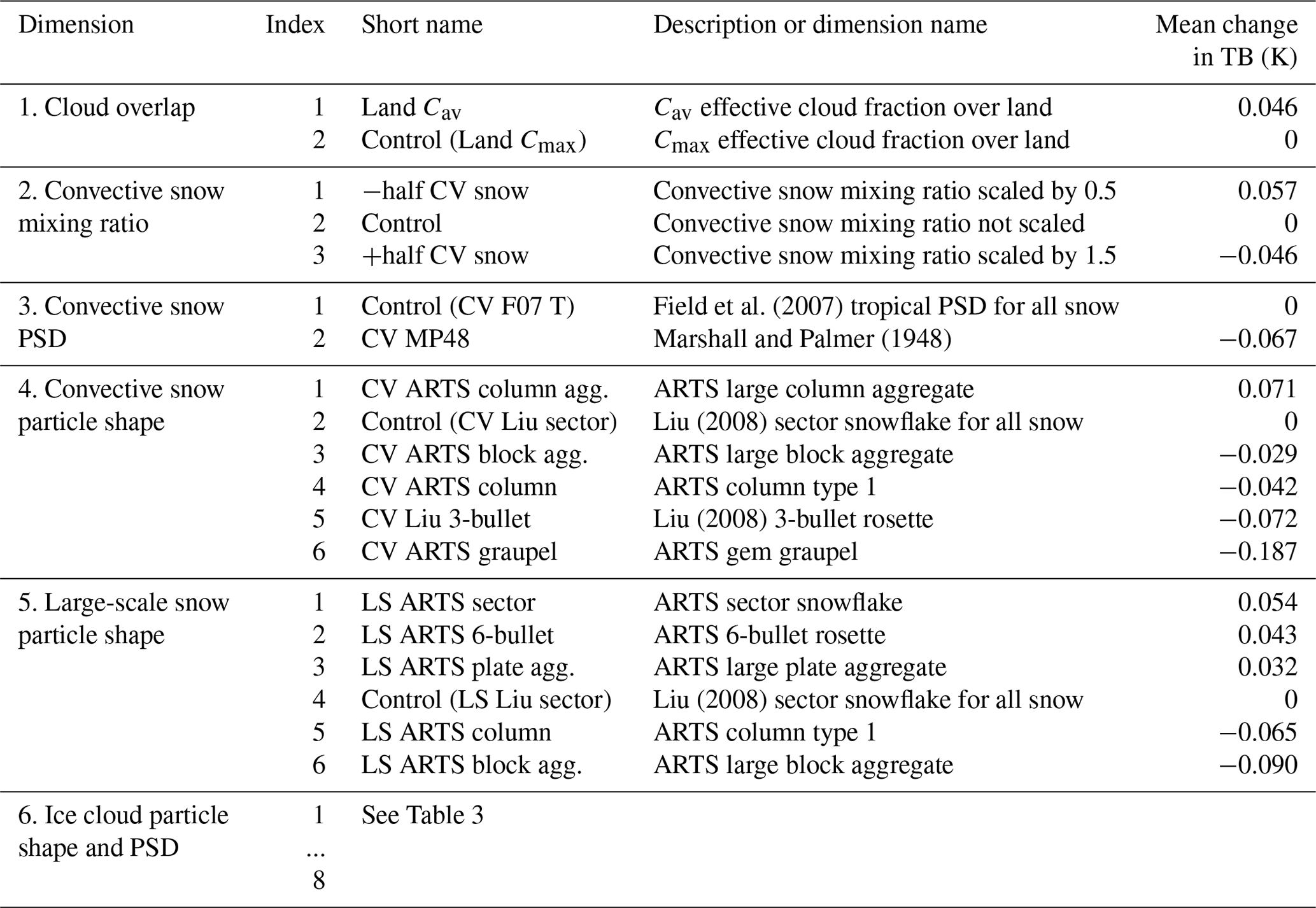
This section will outline the six dimensions of the parameter search, summarised in Table 2. This is a search among discrete possibilities, so the total number of possible configurations is the product of the dimension sizes: . Along each dimension, Table 2 orders the options according to the all-channel global mean change in simulated brightness temperature when that parameter is varied. The main impact of frozen hydrometeors at microwave frequencies is to scatter radiation, which generally leads to lower brightness temperatures at the top of the atmosphere. Hence the dimensions are ordered from the least-scattering options (which increase brightness temperatures compared to the control) to the most scattering (which decrease them). The biggest increase in scattering of any of the options is the move to a convective graupel particle shape, which reduces brightness temperatures globally by 0.187 K. Such global mean changes are obviously small, but this is because cloud and precipitation are localised processes. In heavy precipitation there are still changes of up to around 100 K, as will be illustrated later; see also e.g. Geer et al. (2021) for further illustration of the very strong sensitivity of simulated brightness temperatures to microphysical assumptions.
Field et al. (2007)Marshall and Palmer (1948)Liu (2008)Liu (2008)Liu (2008)Table 2Possible microphysical and macrophysical changes. For details, see text.
Although it would be tempting to add more dimensions to the parameter search, it soon becomes cumbersome and would ultimately become impossible due to the curse of dimensionality. The range of options already encompasses research that will take many pages to summarise. More dimensions could have been included, particularly in the forecast model physics, but that is out of scope of the current study.
3.1 Cloud overlap over land
As described in Sect. 2.2, sub-grid variability of cloud and precipitation has a huge effect on the simulated brightness temperatures. This is represented by the effective cloud fraction C in the two-column approach used by RTTOV-SCATT (Eq. 1). Over ocean, C is computed as a hydrometeor-weighted vertical average of the hydrometeor fractions (Cav), which is a reasonable approximation to more accurate multiple-independent column models (Geer et al., 2009a, b); this remains fixed in the parameter estimation. But over land surfaces, C has previously been set to the maximum cloud fraction in the profile, Cmax, not because this is the most physically correct approach but to counter systematic errors: Geer and Baordo (2014) took advantage of the fact that Cmax generates artificially high scattering TB depressions to compensate for the apparent lack of convective cloud and precipitation over land in the IFS, as seen at frequencies from the microwave to the infrared (e.g. Geer et al., 2019). The hope is that the parameter search can find a configuration that does not require a physically unjustified representation of cloud overlap over land.
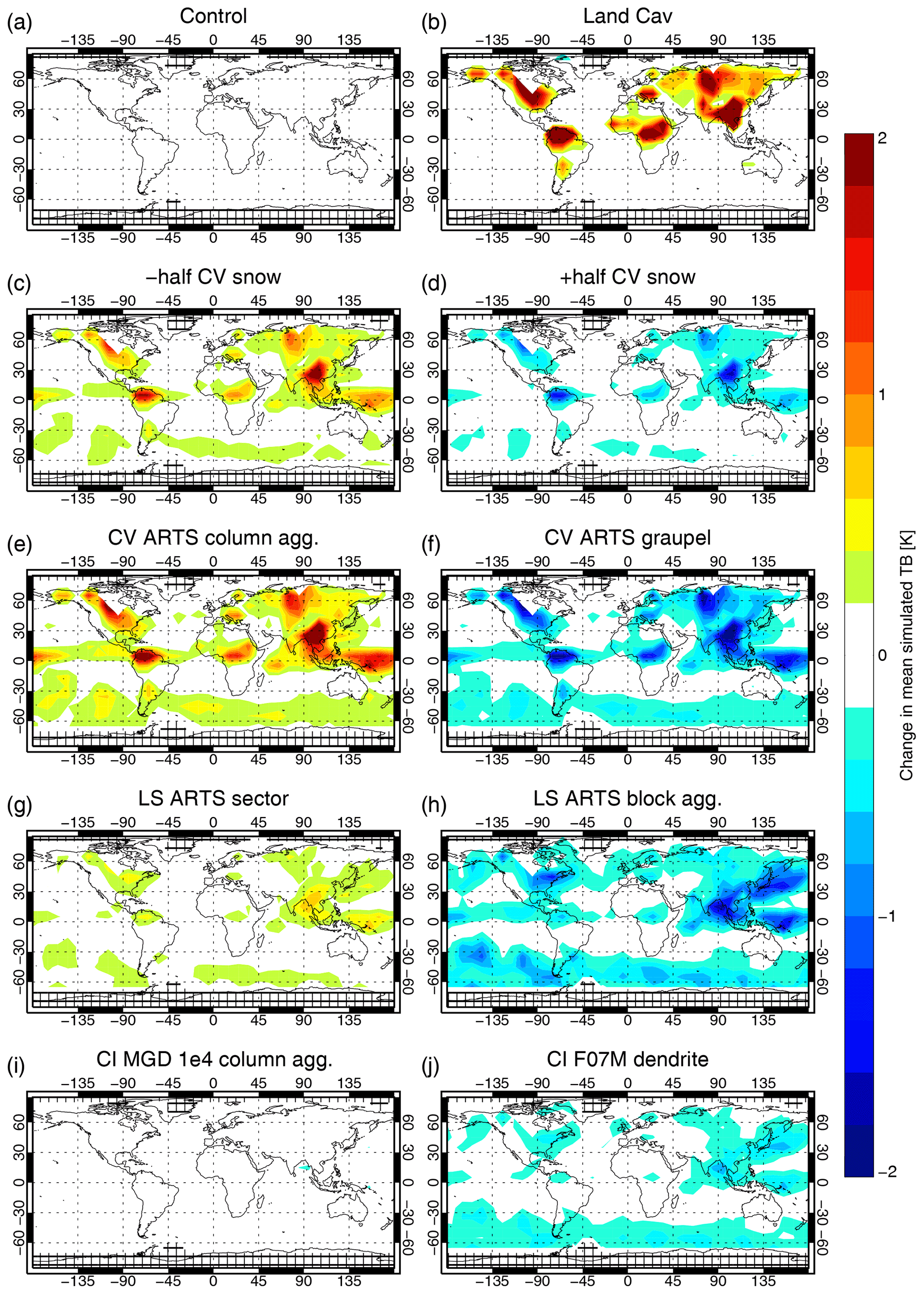
Figure 2Mean change in simulated brightness temperatures when using some of the options from Table 2, compared to the control. Statistics are based on a 10 d period and shown for SSMIS channel 150h, which is generally the channel with the largest impact from changes in the physical assumptions for frozen hydrometeors.
The choice of effective cloud fraction over land affects mainly deep convective situations. In the IFS, convective locations are represented by a convective core occupying 5 % of the model grid box; the anvil is represented by detrainment into the large-scale cloud scheme, which typically results in a thin capping ice cloud with a cloud fraction that is close to 1. In the computation of Cav, the convective core typically dominates the mass-weighted average, and hence Cav can be as low as 0.05 in convection. By contrast the maximum cloud fraction Cmax is typically found in the anvil cloud and is typically closer to 1. Hence, using Cmax in Eq. (1) gives more weighting to the cloudy column and generates much deeper TB depressions. Figure 2b shows that going to Cav increases the mean simulated brightness temperature in many land-surface areas. These locations are similar to those affected by increasing convective snow amount (Fig. 2c, d; see next section), confirming that it is mainly convective situations affected.
3.2 Options for convective snow
The physical parameters of convective snow are not well known and may explain many of the largest errors in the observation operator. In addition, the model-derived convective snow mixing ratio is quite uncertain. One source of uncertainty already mentioned (Sect. 2.2) is the conversion from convective mass flux to mixing ratio, which makes assumptions on the PSD and the fall-speed distribution. The assumed fall speeds are suspected of being too low for convective particles (Geer et al., 2017a, Sect. 3.3). This could lead to convective snow mixing ratios being overestimated by about 50 %. However, as discussed in the previous subsection, the observational evidence from all-sky infrared assimilation is consistent with the convective mixing ratio being too low, particularly over land (Geer et al., 2019). This could come from known deficiencies in the convection scheme, such as insufficient convection at night over land (Bechtold et al., 2014). To simplify the current parameter estimation, it was not attempted to address these uncertainties at their physical source but to treat the convective mixing ratio as an uncertain parameter. Dimension 2 of the parameter search (Table 2) allows the model-derived convective snow mixing ratio to be increased or decreased by 50 %. This scaling is applied across the whole vertical profile. Figure 2c and d show the impact on mean brightness temperatures and reveal the locations where significant convection occurred during the 10 d study period: around the ITCZ, in the SH storm tracks, and at midlatitudes over land surfaces. Adding the convective mixing ratio as a parameter is not intended to provide a scaling factor to be included in a future observation operator but instead to explore the robustness of the results to one of the biggest uncertainties and to point to areas needing future improvement.
Turning to the other convection-related parameters, large hail particles are important in the generation of extreme brightness temperature depressions (e.g. Zipser et al., 2006). Intense convection can generate hail in excess of 127 mm in size (Allen et al., 2017); direct observations from within severe convection are difficult, but an armoured research aircraft has been able to sample PSDs of hail up to 50 mm in size (Field et al., 2019). Hence, dimension 3 of the parameter search (Table 2) explores the convective snow PSD. The control uses the Field et al. (2007, F07) tropical (T) PSD for all frozen precipitation. However, this was derived from in situ measurements of tropical anvils and midlatitude stratiform clouds, so it may not be appropriate for the large frozen particles within the convective cores. The Marshall and Palmer (1948) PSD is provided as an alternative in the parameter search; as implemented here this boosts the number of large particles (≥ 10 mm) by at least 2 orders of magnitude compared to the F07 PSD and hence gives more scattering (see Geer et al., 2021, for more details). The effects of this are not illustrated as they are broadly similar to increasing the convective snow mixing ratio by 50 %.
Another potential adjustment for convective snow is the particle shape. Note that the particle shape also implies a mass–size relation, and hence this affects the bulk scattering properties through adjustments to both the size distribution and the single-scattering characteristics (Eriksson et al., 2015; Geer et al., 2021). The Liu (2008) sector snowflake is used in the control, since this was the best particle to represent the sum of convective and large-scale snow in the parameter search of Geer and Baordo (2014). However it is an idealised smooth and solid particle that will be inadequate to represent scattering in future sub-mm applications (Fox et al., 2019). The ARTS database offers new options of ice aggregates and graupel, and these may be more physically representative (Eriksson et al., 2018). Hence in the fourth dimension of the search, particle types have been chosen to sample different levels of scattering and also some very different physical representations: the ARTS column aggregate4 generates less scattering than the Liu sector, whereas the ARTS block aggregate, column, and gem graupel generate increasingly more scattering. The options also include the Liu (2008) 3-bullet rosette, which was found by Geer and Baordo (2014) to give the best results when convective snow was represented separately to large-scale snow. It is striking that the particle shape assumptions illustrated in Fig. 2e and f have a larger impact on the simulated TB than a 50 % change in the mass mixing ratio (as seen in Fig. 2c and d).
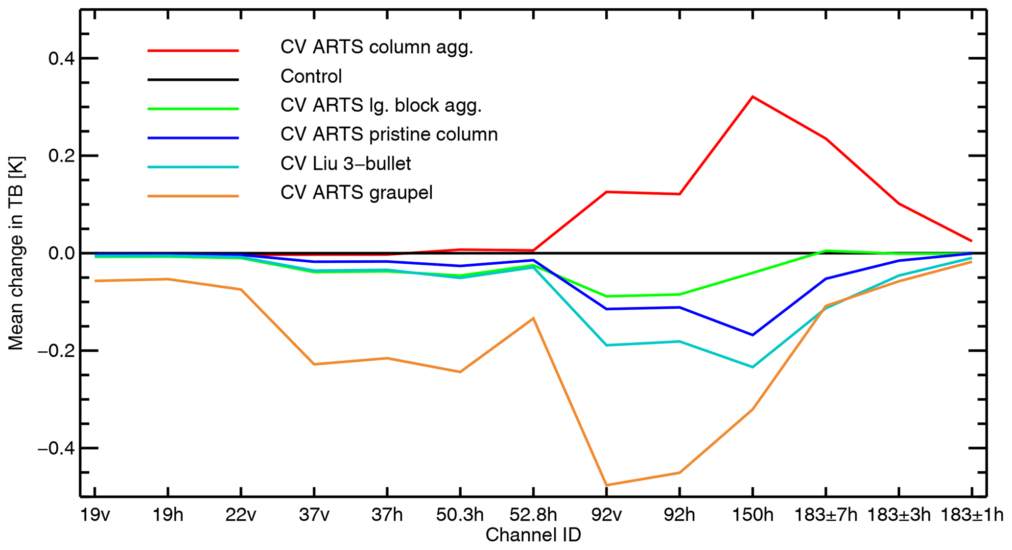
Figure 3Global mean change in simulated brightness temperature when using different options for the shape of convective snow, compared to the control in which the Liu sector snowflake is used for all snow.
Figure 3 illustrates the frequency-resolved global mean change in brightness temperature coming from changes in convective particle shape. Graupel generates significantly increased scattering down to 19 GHz and has its biggest effect around 92 GHz. The other chosen particles do not change the results so much at frequencies below 92 GHz, but there is plenty of variability in the higher frequencies. For example, the ARTS column and ARTS block aggregate would reduce TBs by similar amounts at 92 GHz, but they have different effects at 150 GHz. Hence there is a spectral signature associated with the snow particle shape that should help resolve any ambiguity with changes in mixing ratio. For further illustration of the spectral signatures of these particles, see Geer et al. (2021); in heavy cloud situations these choices can change the simulated brightness temperature by up to 150 K.
3.3 Options for large-scale snow
The representation of large-scale snow is not perfect but probably better than that of convection. Hence only a single dimension is explored – that of particle shape, as shown in Table 2. The Field et al. (2007) tropical PSD was retained for large-scale snow in all experiments, mainly to reduce the search space, but also because this PSD is well established in this context (e.g. Fox et al., 2019). Among the particle shape options, the ARTS sector snowflake is a separate option to the Liu sector snowflake from the control, and it generates warmer mean brightness temperatures (see Geer et al., 2021; this is due to differing mass–size relations; the single-particle optical properties are near identical). The ARTS column and ARTS block aggregate generate more scattering and lead to colder brightness temperatures.
Figure 2g and h show the geographical effect of changing the large-scale snow particle shape. This highlights areas of significant large-scale precipitation during the 10 d study period, including the SH storm tracks, the western Pacific and the Atlantic coast of North America. Although there is some overlap with the spatial pattern of convection seen in Fig. 2c and d, there are also distinct differences – for example in North America, convection dominates over the midwest and large-scale precipitation over the Atlantic coast. This suggests that the convective and large-scale physical parameters should be independently identifiable through their spatial signatures. And as with the convective snow particle choices, there is also spectral differentiation between the large-scale snow shapes that should further improve identifiability (see Geer et al., 2021).
3.4 Options for cloud ice
The current representation of ice cloud in RTTOV-SCATT uses a Mie sphere combined with a gamma PSD and is physically unrealistic (Geer and Baordo, 2014). Ice cloud is expected to have a small effect on radiances at 183 GHz (e.g. Hong et al., 2005; Doherty et al., 2007), but in the control configuration it has almost no effect (not shown). However there is sensitivity at 183 GHz and below (Geer et al., 2021), so it is hoped to find a baseline representation of ice cloud that can be further improved once ICI has been launched.
McFarquhar and Heymsfield (1997)Heymsfield et al. (2013)Heymsfield et al. (2013)Field et al. (2007)Liu (2008)Field et al. (2007)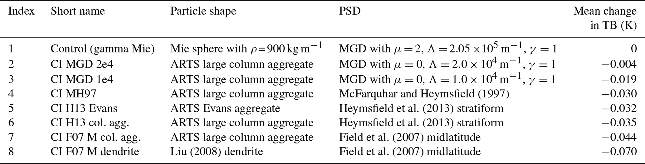
Table 3 summarises the ice cloud options in the parameter search, and further details can be found in Geer et al. (2021). The highest-scattering option is the combination of the Field et al. (2007) PSD and Liu (2008) dendrite, similar to the configuration which gave the best results for ice cloud in the fine search of Geer and Baordo (2014) but using the F07 PSD midlatitude option (M), rather than tropical option, to reduce the number of large particles. Figure 2j shows this configuration decreases brightness temperatures in many areas compared to the control. However, preliminary experimentation suggested there was too much scattering in this configuration. It is only with the new particle shapes and PSDs in RTTOV-SCATT that lower-scattering options have become available (Geer et al., 2021). From the ARTS particle database, the ARTS column aggregate and the Evans aggregate generate less scattering. Also a range of alternative PSDs help reduce the number of large particles and hence reduce the overall amount of scattering. As shown in the table, progressively less scattering can be generated using the McFarquhar and Heymsfield (1997, MH97) and Heymsfield et al. (2013, H2013) PSDs. Early attempts at the parameter search suggested that even less-scattering options might be required, so two ad hoc PSDs were created using the all-purpose modified gamma distribution (MGD; Petty and Huang, 2011); these are known as the MGD 2e4 and MGD 1e4 PSDs, with the number referring to the lambda parameter in the MGD. The configurations using these PSDs make only small changes compared to the control (e.g. Fig. 2i).
Figure 2j shows that ice cloud effects can be seen in convective and large-scale areas alike, so ice cloud has its own distinct spatial signature; there are also some frequency signatures (such as differences between the MH97 and H2013 options, thought to be due to different temperature dependences in the PSDs, not shown). Hence there is hope that ice cloud parameters will be identifiable in this work.
4.1 Search
There are 3456 different parameter combinations available, and it was not feasible to evaluate every combination directly, since each would require a passive monitoring run of the IFS. Instead the cost function was evaluated approximately at each point in the search space. This was done using an assumption of linearly additive perturbations, which will be justified a posteriori. This meant that only one experiment needed to be run for each of the parameter options described in Sect. 3, in addition to the control – a total of 22 experiments. An alternative to running the full IFS would have been to archive the necessary geophysical inputs to RTTOV-SCATT for around 106 observations, but significant storage and computation resources would still have been needed.
The assumption of linearly additive perturbations is expressed mathematically as
Here, T is the simulated brightness temperature, i the index across the approximately 106 observations, and j the index across the 13 selected channels of SSMIS. k is the index across six search dimensions and vk the index within each search dimension. v is a vector containing the six vk indices. Tcontrol is the brightness temperature simulated in the control experiment. As an example, the “intermediate” configuration from Sect. 5.4 is
In the parameter search, the effect of these choices on the brightness temperature was estimated as follows, using Eq. (2):
Note that for simplicity the i and j indices have been dropped here.
Figure 4 illustrates the validity of the linear assumption for the intermediate configuration. This is a scatter plot based on the left and right sides of Eq. (4) after subtracting TControl. The estimate falls around 30 % below the 1 : 1 line for the largest perturbations (≥ 10 K); these points are located in convective land areas (not shown), suggesting that the two convection-related changes (Land Cav and CV Liu 3-bullet) do not combine linearly, which can hardly be expected. However, the estimate has errors mostly less than 2 K for smaller perturbations. The standard deviation of the difference between the estimated and actual perturbation is 0.96 K, suggesting that the assumption is valid to reasonable accuracy in most situations. On maps, the linear-estimated and nonlinear-computed results are surprisingly difficult to tell apart by eye (not shown; this applies both to the brightness temperatures and the binned statistics like those used in the cost function, Sect. 4.2). Similar levels of accuracy have been seen with other configurations. However, for the same reason the assumption is needed in the first place, it is hard to test it exhaustively; possible future improvements are discussed in the conclusion.
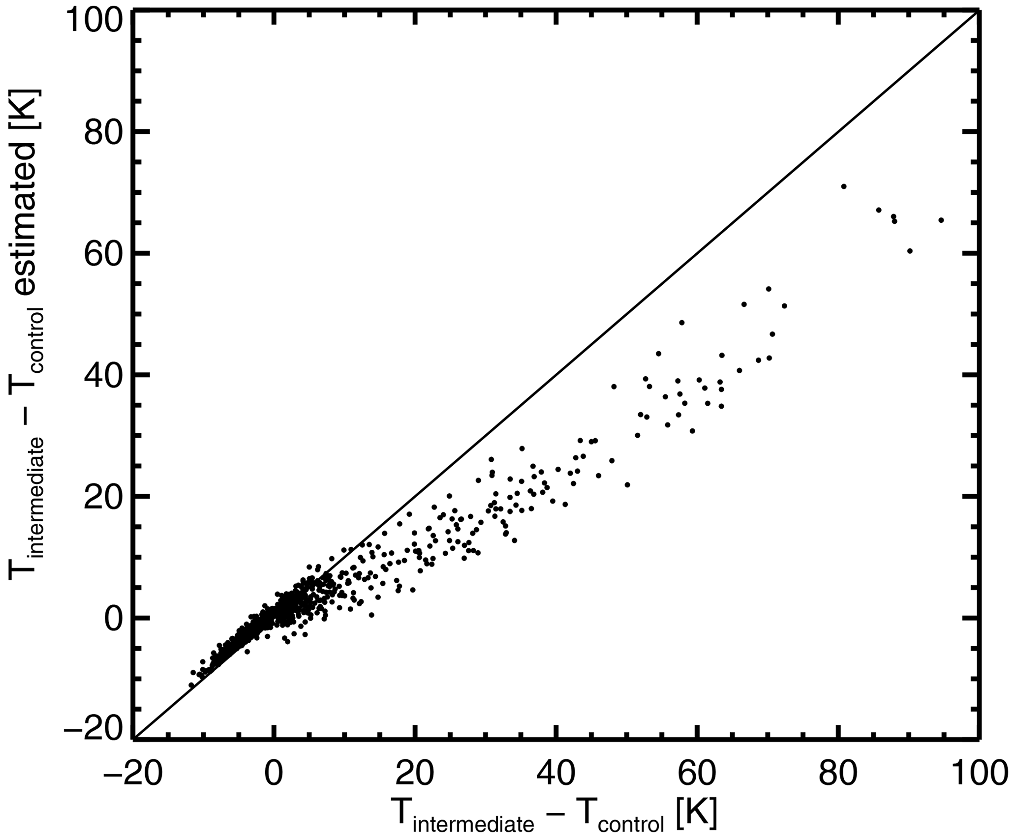
Figure 4Scatter plot of change in channel 92v brightness temperature, relative to control, when going to the “intermediate” physical configuration from Sect. 5.4 (Land Cav, CV Liu 3-bullet, LS ARTS sector, CI H13). On the y axis this is estimated using the assumption of linearly additive perturbations, by subtracting TControl from Eq. (4). On the x axis the intermediate configuration has been evaluated by running an experiment with exactly that configuration.
4.2 Cost function
In order to choose a unique “best” configuration, there must be a single objective way to measure the fit between the model and the observations. Following the data assimilation approach, this is provided by a cost function based on the departure d between the observation and the simulated equivalent:
Here bi,j is an observation bias correction estimated using variational bias correction (VarBC, Dee, 2004; Auligné et al., 2007) within the weather forecasting framework, which will be discussed shortly. In a data assimilation cost function, the equivalent “observation term” is usually based on the square of the departure normalised by the observation error, following an assumption of Gaussian errors (see e.g. Geer, 2021). The best fit to observations, known as the analysis, is obtained where the cost function has a minimum.
The square of the departure is a poor choice of cost metric when it comes to cloud and precipitation. One reason is that modelled and observed clouds are not always in the same place, so it is often possible to reduce the squared error by removing the simulated cloud or precipitation – this is known as the double-penalty effect. As explored by Geer and Baordo (2014), more appropriate cost functions for cloud and precipitation parameter estimation could include the mean and skewness of departures, or measures of fit between the observed and simulated probability distribution function (PDF) of brightness temperatures, using measures similar to the Kullback–Leibler divergence (Kullback and Leibler, 1951). The PDF divergence approach was not pursued here because it is hard to combine with geographical binning (see below) which is used to help make the parameters more identifiable. A vastly larger dataset would be needed to ensure good sampling of the brightness temperature PDFs in each geographical bin.
In order to have a single cost function to minimise, a combination of the mean and skewness of the departures was chosen for the current parameter estimation. Section 5.2 explores alternative choices. The mean and skewness are computed in 10∘ by 10∘ latitude–longitude bins (Fig. 1). Then the absolute value in each geographical bin is combined, giving the following cost function:
Here l is an index over all n geographical bins that contain data (bins with 10 or fewer observations are ignored), |⋅| computes the absolute value, Binl(⋅) represents the geographical subset of observations in bin l, Mean(⋅) computes the mean of a set of departures, and Skew(⋅) computes the skewness (with zero being a perfectly symmetric PDF of departures). The inner sum is over geographical bins, and the outer sum is over the m selected SSMIS channels j. The aim of the parameter search is to find the set of physical choices v that minimises the cost function J(v).
The form of cost function in Eq. (6) has a number of advantages. A single global mean is of little use, since it allows different situation-dependent biases to be summed together. A set of physical choices leading to compensating systematic errors could score as well as a set with smaller systematic error. As illustrated in Fig. 7, geographical separation helps to implement an approximate regime-based separation – for example the errors over tropical land surfaces are separated from those in frontal cloud in the storm tracks and cannot compensate for each other. It is also helpful to compute the skewness in geographical bins, as this measure can otherwise be dominated by the large departures in the vicinity of tropical convection. As will be seen later, this is a significant advance on the use of a global skewness by Geer and Baordo (2014) because it helps identify problems with the use of Cmax over higher-latitude land surfaces, an issue that was missed in the earlier work.
Unlike a typical data assimilation cost function, the error in the observations is not considered in Eq. (6). It is assumed that given the large numbers of observations in most bins (Fig. 1), the mean or skewness of the binned sample is mostly insensitive to observation error. Normal data assimilation also includes a background term measuring the deviation from prior knowledge, and also serving to regularise the problem. Section 6.2 discusses the issue of prior knowledge further, and regularisation is not needed as the problem is likely to be well determined, with six unknowns and around 106 observations.
The VarBC bias correction, bi,j in Eq. (5), is fixed throughout the passive monitoring experiments conducted here. A large part of the modelled bias, especially for SSMIS, is thought to come from the instrument calibration, so it is necessary to include a bias correction. VarBC estimates the bias as a linear combination of a globally constant offset, a number of polynomial terms based on the instrument's scan angle, and a number of model-based predictors. For surface-sensitive observations over ocean, these include the total column water vapour (TCWV), skin temperature, and surface wind speed. For sounding channels, they include functions of the layer thickness (an average temperature, essentially). None of the predictors is directly correlated with cloud-related biases, so these do not map directly onto the VarBC bias correction. In some channels the bias correction aliases some of the latitude-dependent biases, such as differences between tropical and midlatitude cloud simulations, but the effect is generally small. Ideally VarBC would be allowed to vary, but as a first approximation it is held constant.
5.1 Global parameter search
The first application of the parameter search is to find a single set of physical parameters that would provide the best fit globally, a one-shape-fits-all approach. Figure 5 helps to visualise the six-dimensional cost function by showing slices along its dimensions at the control configuration and at the best configuration. At the control configuration, perturbations in most directions would increase cost: for example, all other choices of convective snow particle would make things worse. This indicates that the configuration provided by Geer and Baordo (2014) was already at a reasonably stable local minimum.
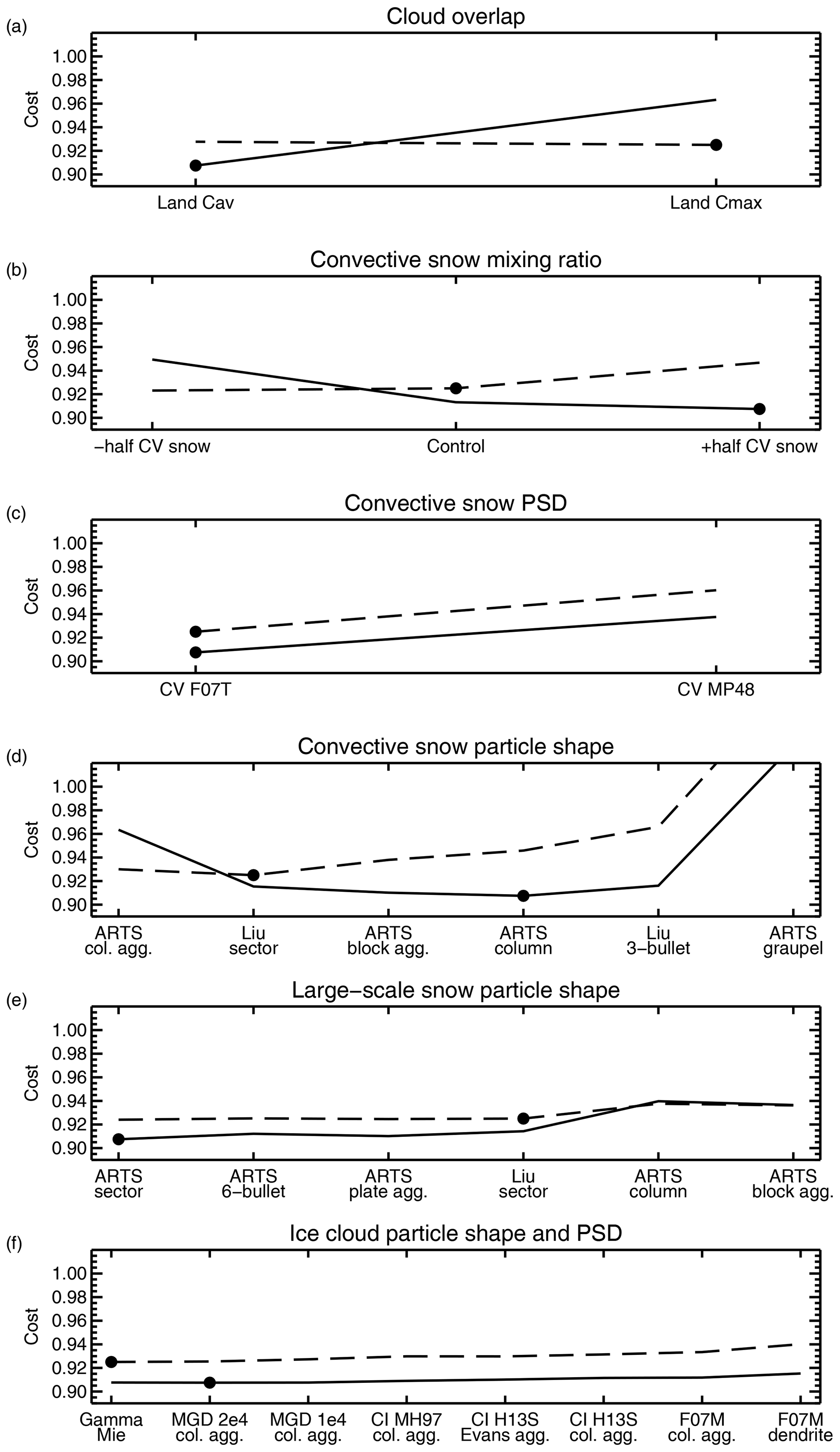
Figure 5Slices through the six-dimensional cost function around the control configuration (dashed) and around the best configuration (solid; see also Table 4). The dimensions are ordered from least-scattering to most-scattering options. The dots indicate the parameter settings for the control and for the very best (lowest cost) configuration.
The best configuration is summarised in Table 4. Here, the shape of the cost function is very different (Fig. 5). The largest difference is the reversal in the gradient of the cost function with respect to cloud overlap. Cav overlap over land is now clearly better than the Cmax overlap used in the control. Another big difference is that the choice of convective snow particle is now well bounded at the extremes: at low-scattering the ARTS column aggregate has high cost and is clearly inappropriate; at the high-scattering end the ARTS graupel also gives a high cost. The ARTS column is marginally the best, but the ARTS block aggregate or Liu 3-bullet would be a reasonable alternative. A final big difference is the change in the gradient of the cost function with respect to convective snow mixing ratio. At the best configuration, the mixing ratio should be increased by 50 %, whereas the control configuration could have been improved by reducing the mixing ratio by the same amount.

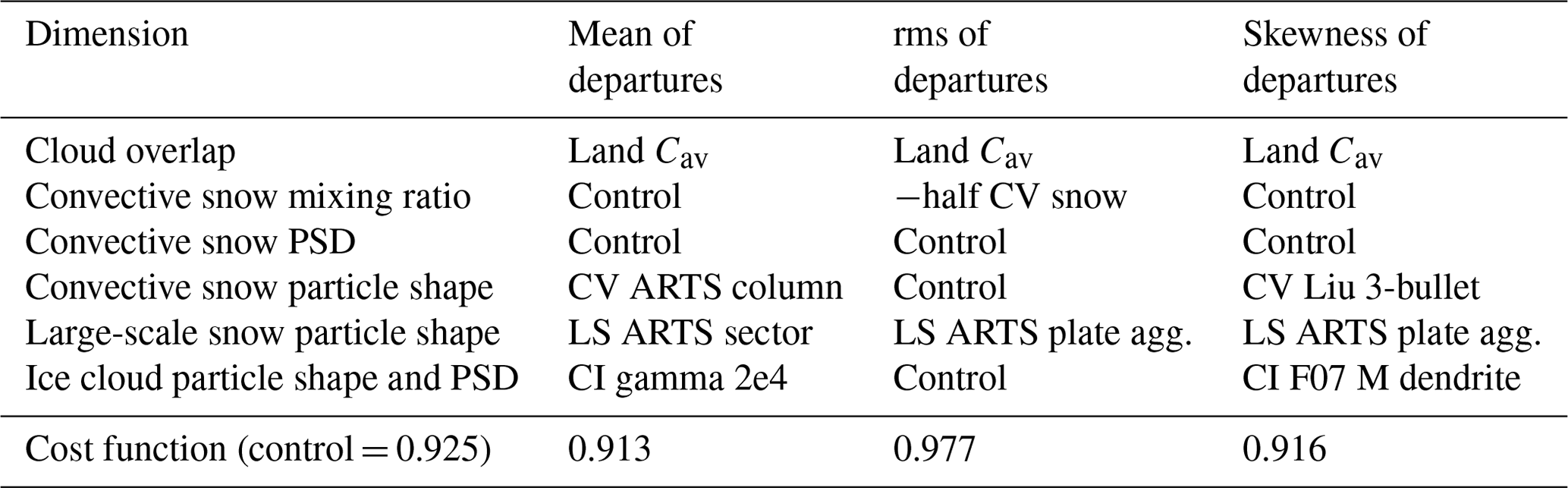
There are smaller changes in the other dimensions in Fig. 5. For the large-scale snow, a small improvement is found going to the ARTS sector, although the ARTS 6-bullet, ARTS plate aggregate, or Liu sector (the control configuration) would produce similar results. The lower-scattering end is not bounded, so it might be possible to further improve the simulations with a less-scattering configuration for large-scale snow. The least constrained dimension is the ice cloud microphysics: all configurations produce similar cost, with the MGD 1e4 PSD being only marginally better than the others. Only the F07M PSD with the Liu dendrite shows a visibly increased cost; as previously mentioned this was identified in initial work as having too much scattering. Table 4 summarises the best global configuration: overall this reduces cost to 0.908, compared to 0.925 at the control. This is only a small improvement, despite major adjustments to the parameters. As will be seen, these adjustments bring a mix of improvements and degradations that is overall just slightly better according to the cost function. Section 5.2 will show that bigger improvements can only come about by making the parameters situation-dependent.
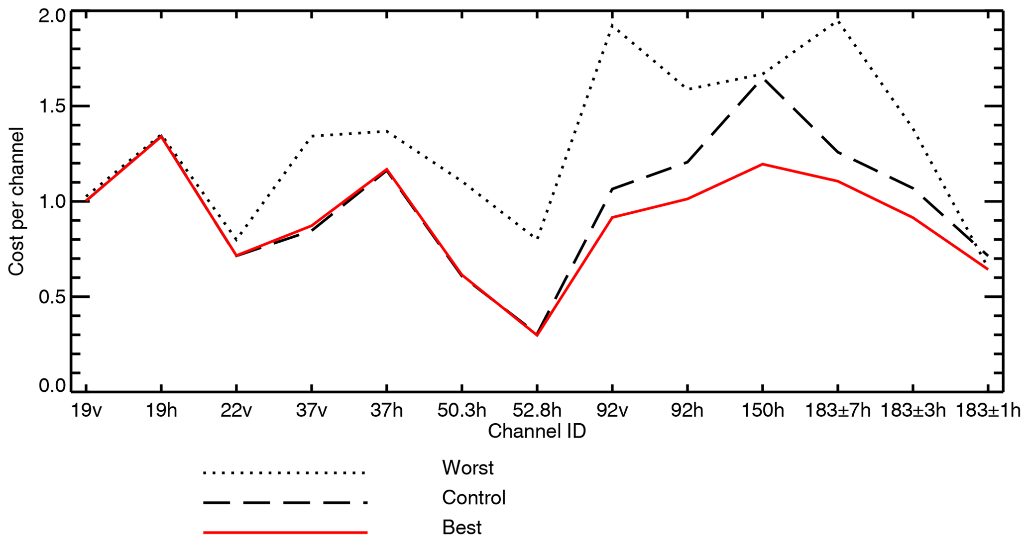
Figure 6Cost per channel of different sets of physical options in the parameter estimation. Shown are the configurations with the smallest and highest cost (best and worst) and the control.
Figure 6 examines the cost function broken down by SSMIS channel. The best option improves the fit to observations (reduced cost compared to control) in channels from 92v to 183 ± 1h. This can be contrasted with the worst possible option in the parameter search (the dotted line) which makes the cost higher in channels down to 22v. The worst possible option chooses all the most-scattering options available, such as the ARTS gem graupel particle for convective snow, and generates significantly increased scattering at low frequencies (20 to 50 GHz; see also Fig. 3), which does not agree with observations; this was also one of the problems with the Mie sphere snow representation rejected by Geer and Baordo (2014). The high-scattering options, including the ARTS graupel and the Mie sphere, tend to put deep TB depressions everywhere there is convection. But in the observations, deep scattering TB depressions are seen at these frequencies only in the very most intense convection (e.g. Zipser et al., 2006). The new search continues to constrain the choices to those that have relatively low scattering at the lower frequencies, while still being able to produce significant scattering at higher frequencies. This illustrates the importance of including the lower frequencies in the cost function.
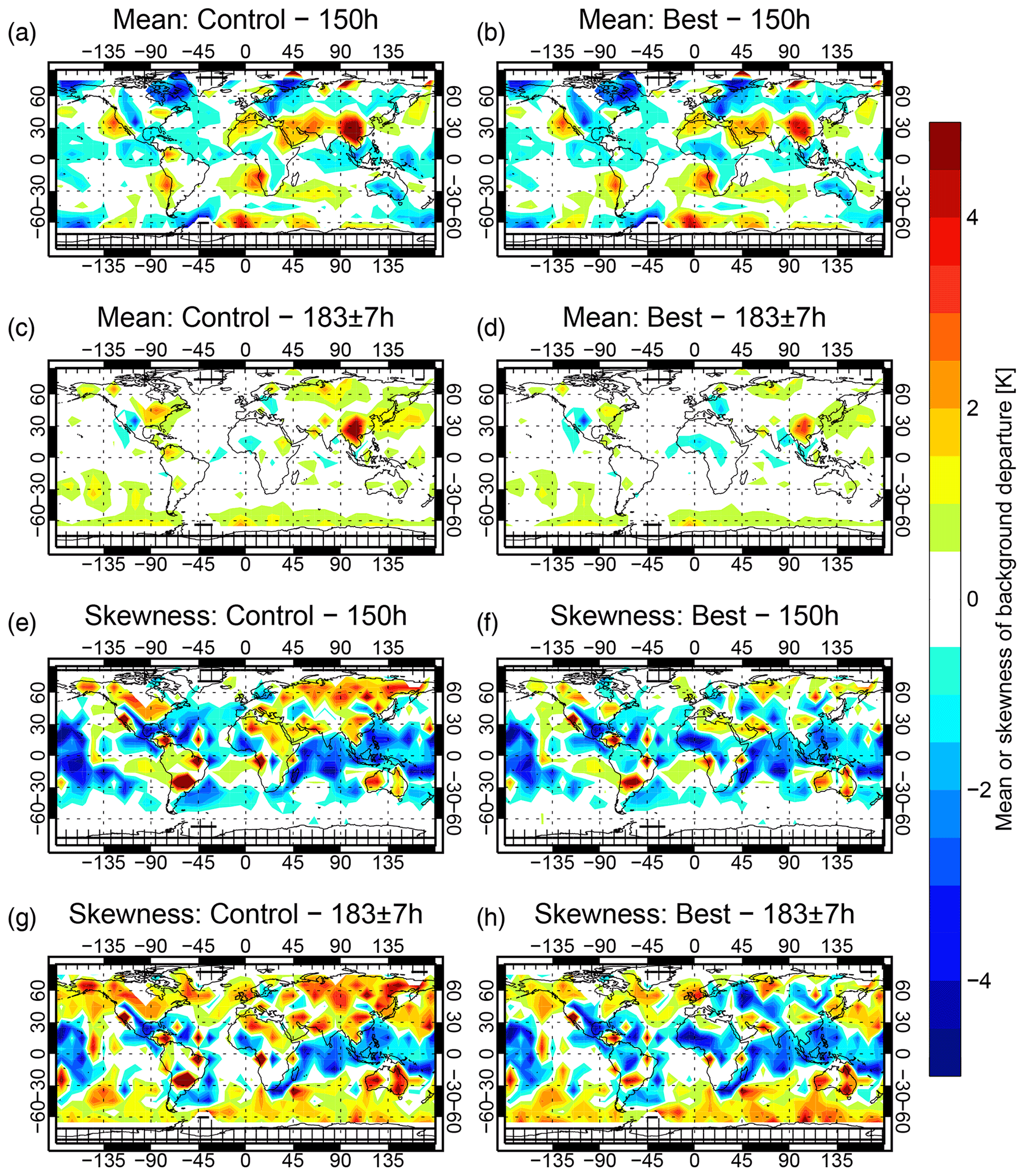
Figure 7Maps of mean and skewness of background departure in the control and in the best configuration.
Figure 7 shows maps of the mean and skewness of departures in the geographical bins that make up the cost function (Eq. 6). The best option improves the mean of binned departures over extratropical land surfaces, particularly in the NH at 183 ± 3 GHz. The skewness of binned departures in the control is around +3 in many of these areas; the best option reduces skewness mostly to the range −1 to +1, at both 150 GHz and 183 ± 3 GHz. However, some areas show worse levels of skewness. For example, there is more negative skewness in the ITCZ over central Africa at 150 GHz and 183 ± 3 GHz and slightly more positive skewness over the Southern Ocean at 183 GHz. To better understand these changes, Fig. 8 shows the histograms of brightness temperatures at 150 GHz over land, separated into broadly extratropical and tropical areas using a TCWV threshold. In extratropical locations the control has an order of magnitude too many occurrences of strong scattering (TBs less than 210 K) compared to observations, and the “best” configuration provides a much better distribution. This change is consistent with the move from positive to neutral skewness in extratropical land areas in Fig. 7. It is mainly the result of changing from Cmax to hydrometeor-weighted Cav cloud overlap over land surfaces.

Figure 8Histograms of SSMIS 150h brightness temperatures over land surfaces (greater than 0.5 land fraction): (a) locations with less than or equal to 25 kg m−2 total column water vapour (TCWV, approximately 125 000 observations); (b) locations with more than 25 kg m−2 TCWV (approximately 81 000 observations).
In contrast to the improvements over extratropical land surfaces, Fig. 8b shows that in tropical areas an overestimate of strong scattering events has been replaced by a more severe underestimation, consistent with the move to negative skewness in tropical convective areas. This exposes the problem of missing convection that the Cmax overlap had previously helped to hide. The best configuration (Table 4) also includes an increased convective mixing ratio and the move to ARTS column to represent convective snow, both of which significantly increase scattering (Table 2, Fig. 7); however, this is not enough to fully compensate. This worsening of results over tropical land surfaces illustrates the trade-offs required by a global parameter estimation and helps explain why the overall cost has not decreased by much.
Figure 9 illustrates the changes to the simulated SSMIS 150h brightness temperatures over Africa, Europe, and the Atlantic, on a day with a broad variety of cloud and precipitation features across these areas. Brightness temperatures below 240 K over land surfaces typically indicate scattering from convective snow. Simulated brightness temperatures in panels (c) and (d) are similar to the observations in panel (b), but with the exact placement of convection often in different locations – hence the need for a cost function that is resistant to the double-penalty effect. Over land, simulated TBs have increased by up to 100 K (panel a, where the changes are off scale), corresponding to the changes in the TB histograms discussed in previous paragraphs. Over the ocean, there is a general slight decrease in brightness temperatures and hence an increase in scattering. Here, the cloud overlap is not changed, but the other four changes in the best configuration (Table 4) decrease brightness temperatures by up to 5 to 10 K in cloud and precipitation areas, such as convection in the ITCZ around 8∘N, and in an extratropical cyclone in the North Atlantic. These changes are also present in the southern extratropics and are likely responsible for the reduction in mean departures over the Southern Ocean in the 183 ± 7 GHz channel (Fig. 7c and d).
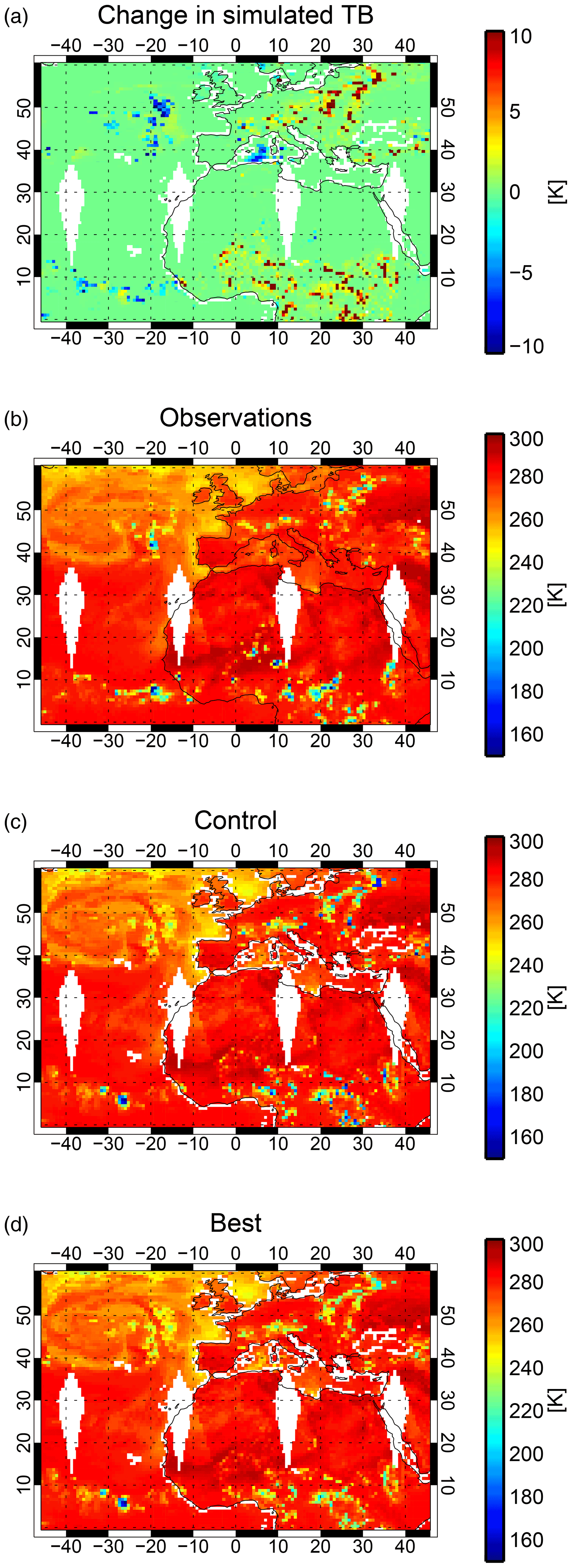
Figure 9Example of SSMIS 150h brightness temperatures on 21 June 2019 (00:00–24:00 UTC): (a) change between control and best configuration; (b) observations; (c) control simulations; (d) best configuration simulations. The colour scale in (a) is optimised to highlight the negative range; positive changes go off scale to as much as 100 K.
5.2 Sensitivity tests
The global best solution from Fig. 5 is fairly stable. Figure 10 shows slices through the cost function around the best solutions that can be obtained with the convective snow mixing ratio fixed to one of the three possible options. Along the dimensions representing cloud overlap, convective snow particle shape, and ice cloud particle shape and PSD, the cost function has a stable form and produces similar solutions in all cases. This suggests that all three choices are reasonably insensitive to the convective snow mixing ratio. However, for convective snow PSD and the large-scale particle, the shape of the cost function, and the best choice, varies depending on the convective snow mixing ratio. In particular the large-scale particle shape has two possible minima – one at the ARTS sector and one at the control (Liu sector) configuration. The latter is found, along with a change to the convective PSD, when the convective snow mixing ratio is halved.
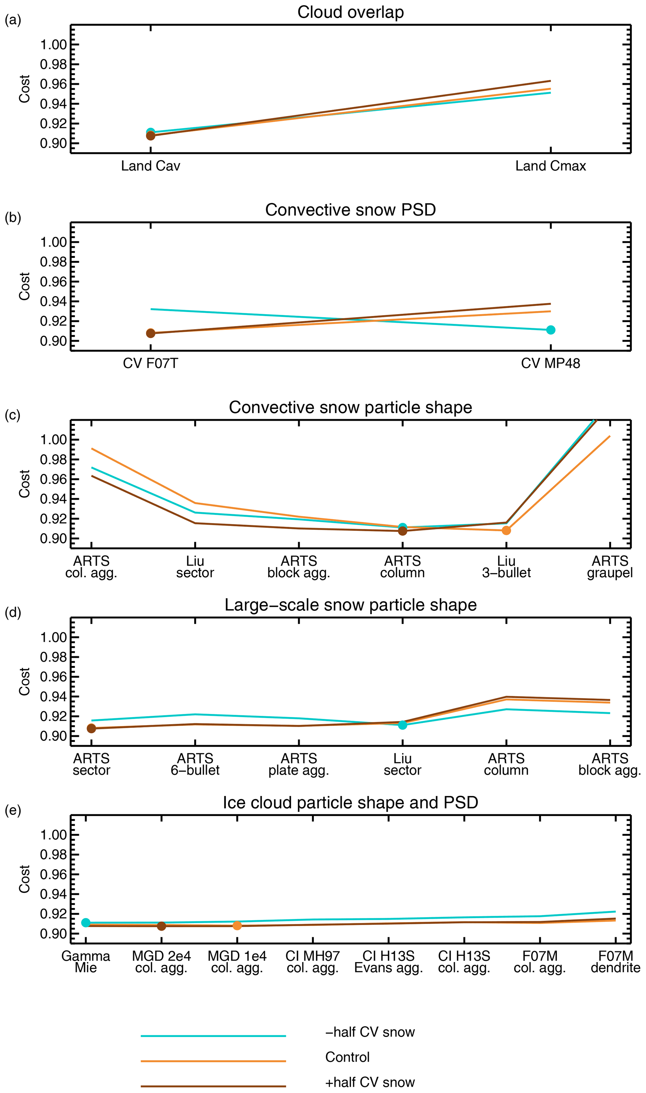
Figure 10Slices through the six-dimensional cost function around the best configuration when the convective mixing ratio is prescribed at −50 %, control, or +50 %. The +50 % lines are the same as the best solution in Fig. 5.
Similar figures can be constructed by holding the choices fixed across any other dimension (not shown). The cost function can be returned to something resembling its shape at control (as seen in Fig. 5) by retaining Cmax hydrometeor-weighted cloud overlap over land or by pushing the large-scale snow to either of the two most scattering shapes. Hence at the broadest scales the cost function has two stable areas giving reasonable solutions, one around the control and one around the new best configuration. Varying the convective snow PSD or the ice cloud particle shape has little effect on the shape of the cost function at solution, which remains close to the new best, further confirming its stability. Finally, setting the convective snow particle shape to the extreme possibilities can generate very different cost function shapes, but these lead to low-quality (high cost) configurations.
Table 5Results of parameter search using alternative cost functions.
The cost given is that of the chosen configuration but calculated with the standard cost function (half mean, half skewness – Eq. 6).
Table 5 explores sensitivity to the choice of cost function itself. The mean and skewness find similar solutions to those found using the average of both (Table 4). On their own they identify some of the reasonable alternative choices, such as the ARTS plate aggregate for large-scale snow, that could already be identified from Fig. 5. Neither the mean nor skewness-based cost function would on its own adjust the convective mixing ratio, consistent with the lack of sensitivity to adjustments in this parameter. A more unexpected aspect of the skewness-based cost function is the choice of the Liu dendrite and the Field et al. (2007) midlatitude PSD for ice cloud, which was identified as a poor choice in early experimentation (it causes significant degradation in observation fits in cycling data assimilation experiments). However, this choice increases the amount of scattering in tropical convective areas, which improves the skewness (figures not shown). The implications are discussed further in Sect. 6.1.
Table 5 also shows the results using a cost function based on the rms of the geographically binned departures. This puts most parameters towards the least-scattering end of the scale, and in particular it reduces convective snow by 50 %. This is not expected to be a valid solution: the double-penalty effect typically means that rms error can be minimised by reducing scattering, essentially by removing cloud from the simulations. This creates a model with an incorrect PDF of brightness temperatures, as measured by the skewness or by examining the PDF directly (not shown). Indeed the cost as measured by the standard cost function is increased substantially to 0.977 at this solution.
5.3 Situation-dependent parameter choices
The global one-shape-fits-all approach has always had trouble getting good results in the tropics and midlatitudes simultaneously (Geer and Baordo, 2014), and the new global solution remains a trade-off with too little scattering in tropical convection and too much scattering in the storm tracks (Fig. 7h). Table 6 summarises the best configurations when the globe is instead divided into three areas: ocean areas outside of tropical deep convection, ocean areas generally in or near tropical deep convection, and land surfaces. The distinction of tropical convection is made roughly using a TCWV threshold of 40 kg m−2 (this identifies a mostly equatorial band covering the ITCZ but extending to around 30∘ latitude in areas like the Pacific warm pool and the South Pacific convergence zone, SPCZ). The non-convective ocean solution is similar to the global solution, which is not surprising given these scenes dominate the global score numerically, but there is an unexpected reduction of 50 % in convective mixing ratio. Compared to Fig. 2, the skewness of background departures is brought much closer to zero at latitudes around 60∘ over ocean (not shown). This is consistent with the conjecture that particle fall speeds in the flux to mixing ratio conversion are too low (Geer et al., 2017a, and see earlier). This also demonstrates the importance of correctly modelling convection even in the midlatitudes.
Table 6Results of a situation-dependent parameter search. “n/a” means not applicable.
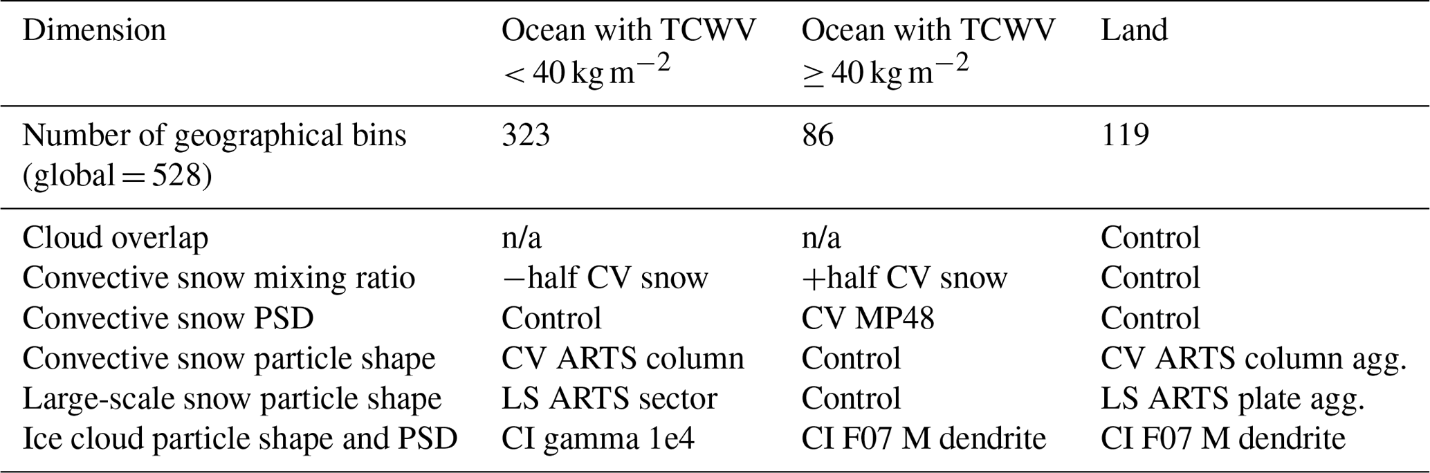
The tropical convective ocean solution is very different to the global solution. There is a 50 % increase in the convective snow mixing ratio and a move to the Marshall and Palmer (1948) PSD. Both of these changes significantly increase the scattering from convection. Further, the ice cloud is represented with the Liu dendrite, which is the most-scattering option. The solution over land is different again, boosting scattering in convective scenes by retaining the Cmax cloud overlap and again using the Liu dendrite for cloud ice. However, the convective and large-scale snow habits themselves move to slightly less scattering options. These solutions both make a substantial increase in the amount of scattering coming from convection, again illustrating that the simulations do not provide enough scattering in tropical areas over both land and ocean (with the problem mitigated over land in the control using an incorrect cloud overlap model). These results will be explored further in the discussion (Sect. 6.1). Using the situation-dependent choices from Table 6, the global cost function could be reduced to 0.886, more than doubling the improvements that were made with the best global solution (Table 4). However, the remaining cost is still high, suggesting many further improvements need to be found.
5.4 Final version for RTTOV v13.0
One drawback of developing models using parameter estimation is that they need to be updated when other components change. Table 7 shows an intermediate and a final configuration for v13.0 of RTTOV-SCATT. The intermediate configuration was found using the same global cost function from Sect. 4, but adjustments to the convective mixing ratio were prevented, being poorly constrained as shown in Sect. 5.2. Also the ice cloud was constrained to a solution using the Heymsfield et al. (2013) PSD, which was initially favoured as the most recent and hopefully most accurate PSD for cloud ice available in RTTOV-SCATT. This configuration is otherwise similar to the global best found in Sect. 4, but with slightly different microphysical choices from within the poorly constrained areas of the cost function (Fig. 5). This configuration was important for testing the other developments towards v13.0. In particular, it was used by Barlakas et al. (2021) to develop a representation of polarised scattering and to tune the required polarisation ratio parameter. In areas affected by strong scattering, the new approach to polarisation increases brightness temperatures by up to around 7 K in vertically polarised channels and decreases them by the same amount in horizontally polarised channels. Since all the high-frequency channels of SSMIS are horizontally polarised (≥ 150 GHz; see Table 1), this alters the reference against which the results in the current work were derived.
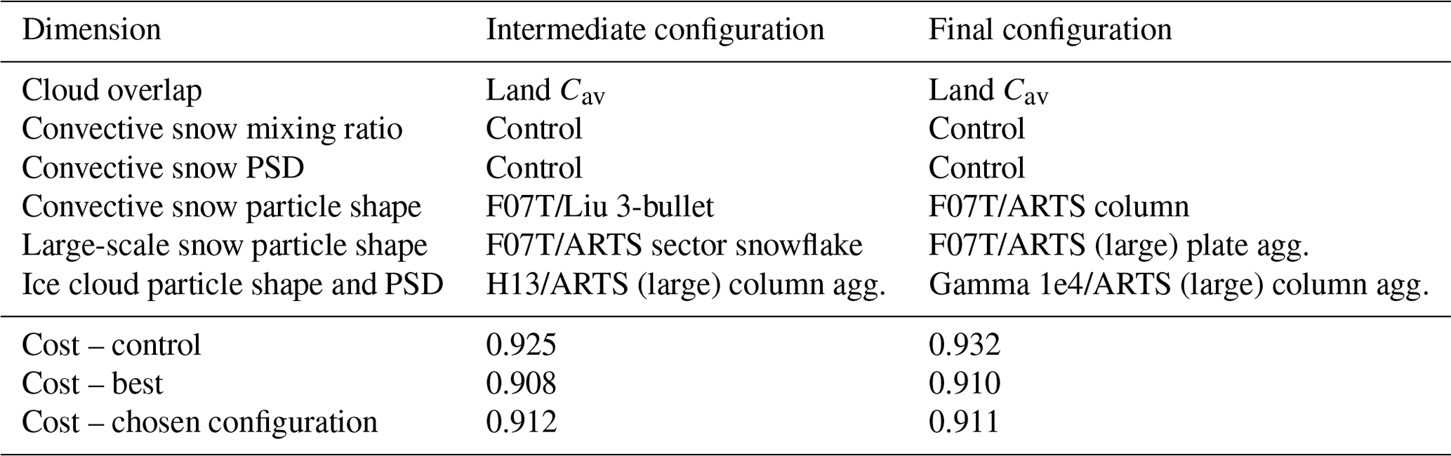
Two other changes were made to RTTOV-SCATT in the late stages of development for v13. First, there was a bug fix to the downward scattering source terms, leading to changes of up to around 1 K in simulated brightness temperatures in some situations. Second, there was a change to the minimum permitted effective cloud fraction, which gave changes mostly within 2 K but occasionally up to around 8 K (for more information on both, see Saunders et al., 2020). Mean changes were an order of magnitude smaller than those examined in typical perturbations in the parameter search (not shown), but, along with the polarisation update, it was important to take these modifications into account in a final re-run of the parameter estimation.
To come up with the final configuration for v13.0, the three late changes were imposed as additional deltas in Eq. (2), relying again on the linear additivity of the changes, which is not significantly affected compared to what is illustrated in Fig. 4. None of the changes was treated as optional, since they all make the radiative transfer more physically correct, and the tunable polarisation ratio parameter could not be constrained in the current work. The additional 3 deltas increased the control cost slightly (to 0.932, Table 7). The convective mixing ratio was held constant, given it is undesirable for future developments to build in a tuning factor in this way, and given the lack of sensitivity to this parameter (Sect. 5.2). Table 7 gives the final chosen configuration, again just a slight perturbation on the best configuration found earlier and still within the uncertainty zone of Figs. 5 and 10.
The final chosen configuration is the best configuration in the parameter estimation, but with an imposed change for cloud ice. The true minimum was found at the control settings for cloud ice (a Mie sphere). Any of the higher-scattering options for cloud ice now generates significantly increased cost, and although the shape of the cost function is similar to Fig. 5f, the gradient is increased (not shown). Hence it is not possible to force the choice of the preferred Heymsfield et al. (2013) PSD any longer. However, the control configuration for ice cloud is undesirable for future sub-mm applications since it uses the outdated Mie sphere approach. A compromise was possible, and the use of the MGD 1e4 PSD with the ARTS column aggregate has been imposed since, after this change, the cost function is only slightly increased.
6.1 Improved physical assumptions
This section discusses whether the parameter estimation has provided physical suggestions that may be generally applicable, or whether the results just reflect tuning to fit the biases of the forecast model used as the reference, and/or the limitations of the radiative transfer model. The biggest improvement was to change the effective cloud fraction over land, which is not surprising as it is the more physically correct approach (Geer et al., 2009a). However, there may be a number of more novel suggestions that could be generally applicable. The first of these relates to convective cloud in the tropics. When the search was confined to land areas (Table 6) it retained the Cmax cloud fraction, despite the fact it is less physical. It is hence worth asking if the specified 5 % convective fraction is too small to represent intense tropical convection systems, noting that even in cloud-resolving models this is an uncertain parameter (e.g. Varble et al., 2014). Radar cross sections can show vertically spreading high-reflectivity areas in the upper parts of these clouds (e.g. Hong et al., 2005, their Fig. 1). Hence a hypothesis, based also on results from cloud-resolving models, is that the frozen upper parts of the convective cores become more widely spread and merge together in a gradual transition to anvil cloud (Geer et al., 2017a). The basic representation of convection in the IFS and RTTOV-SCATT, as a narrow vertical core and a thin high anvil, may therefore be an overly severe truncation of reality.
Further justification for the hypothesis on the structure of intense tropical convection is seen over tropical ocean surfaces in the situation-dependent search (Table 6). The results over ocean are less affected by model bias: here the more physically correct Cav cloud fraction is used, and the all-sky infrared biases suggest only a slight overestimation of convective cirrus in frequency or coverage (Geer et al., 2019). But the parameter estimation still boosts scattering by increasing the convective mixing ratio, by increasing the size of the convective particles using the MP48 PSD, and by making the cirrus more scattering too (using the F07M PSD and the dendrite snow particle). All of these could suggest the need to represent either broader convective cores in the frozen parts of the cloud or, nearly equivalently, deeper convective anvils, containing higher mixing ratios of larger and more scattering particles. Hence an option to improve the results may be to represent convective anvil ice particles as a separate new hydrometeor type for the purposes of radiative transfer.
Another interesting point is the level of constraint on the convective snow particles. At the most scattering end, the ARTS graupel particle is decisively rejected. This is always a bad option, independent of the choice of cloud overlap over land (Fig. 5) and independent of convective mixing ratio (Fig. 10), because it generates too much scattering at lower frequencies. However, the global search finds solutions (such as the Liu 3-bullet or ARTS column) that strongly increase scattering at 150 and 183 GHz and by nearly as much as the ARTS graupel (Fig. 3). The parameter estimation prefers a spectral signature of scattering that is strong around 183 GHz but weak around 50 GHz. This eliminates a wide class of dense particles (Geer et al., 2021) and similarly rejects the least-scattering particles, particularly the ARTS column aggregate, which strongly reduces scattering around 183 GHz (Fig. 3). This spectral signature is hence strong enough to be mostly independent of both the sub-grid structure and the mixing ratio of the convective cloud.
The detectable influence of a particle model in this work is its scattering signature, as a function of frequency and geographical location, and not directly its physical properties. The scattering signature comes from the bulk scattering properties that arise from the combination of particle size distribution and the single-particle scattering properties. In the approach used here the chosen particle model affects both the single-particle scattering signature and the PSD, since the particle choice also defines the mass–size relation. Changing the mass–size relation changes the shape of the PSD (e.g. Eriksson et al., 2015; Geer et al., 2021). In the mass–size relation the ARTS graupel has an exponent of 2.96; the Liu 3-bullet and the ARTS column have exponents 2.37 and 2.05 (Geer et al., 2021). This suggests the scattering signature may be as sensitive to the exponent in the mass–size relation as to the actual particle shape. This would help explain how a habit that is physically unlikely in convection, such as the ARTS column, has ended up being chosen to represent convective snow.
One aspect of convection that is not examined in this study is the presence of supercooled raindrops above the freezing level. These are not represented in the rain and snow fluxes from the model's mass-flux convection scheme, but they are likely there in nature, where they help generate rimed particles and lightning (e.g. Kumjian et al., 2012; Fuchs and Rutledge, 2018). Compared to snow, raindrops are much-less-scattering particles (e.g. Geer et al., 2021) and could generate significant emission, warming the microwave brightness temperatures towards the physical temperature of the cloud and possibly making it harder to generate significant scattering brightness temperature depressions in deep convection. It would be important to address this in future work. Another aspect that could be improved is to use the recently derived hail PSD (Field et al., 2019) to represent the “convective snow” category rather than re-purposing other PSDs.
The results for ice cloud also provide some interesting results for further investigation. The parameter estimation rejected all the PSDs that were explored here as representations of ice cloud (McFarquhar and Heymsfield, 1997; Field et al., 2007; Heymsfield et al., 2013). Note the rejection was much clearer in the final search for RTTOV v13.0 in Sect. 5.4 than in the main search, presumably because the scattering generated by ice cloud had been boosted by the parametrisation for polarised scattering. The PSDs from the literature were trialled with the very-least-scattering particles available to RTTOV-SCATT, i.e. the ARTS column aggregate and the Evans snow aggregate (see Geer et al., 2021). Even so, the observations could only be matched by creating a modified gamma distribution (MGD) with the key property that it generated orders-of-magnitude-fewer centimetre-sized particles than the PSDs from the literature (see Geer et al., 2021). Therefore, although frequencies around 183 GHz are not expected to have strong sensitivity to smaller cloud ice particles, they still impose a constraint on the number of large particles in the PSD.
It is difficult to compare directly to other studies. A main reason is that the characterisation of frozen particles, into large-scale snow, convective snow, and cloud ice, is specific to certain types of global models. It is hard to map onto other representations of ice particle, particularly those in which no forecast model is available to categorise the hydrometeor type (e.g. Ekelund et al., 2020). Further, many studies do not attempt to fit such a range of frequencies or such a complete sample of observations (either in frequency or location), so they are able to find solutions that would not work here. Finally it is worth restating that the results are valid on the 80 km by 80 km smoothing/superobbing grid used for all-sky assimilation in the IFS; hence results may be different from a much-finer-scale cloud-resolving viewpoint. However the following examples based on regional models illustrate that there is plenty of common ground between them and the conclusions from the current parameter estimation.
Guerbette et al. (2016) used RTTOV-SCATT in combination with a tropical local area model to simulate all-sky microwave observations in the tropics around 183 GHz. Their study applies to snow but with a focus on tropical cyclones, so this is interpreted as mapping onto the convective snow category. They tried all the Liu (2008) particles available to RTTOV-SCATT, finding the best fit to observations using the Liu block hex column and the F07T particle size distribution. However they did not include any lower frequencies to help constrain their particle choice. If they had done that, the choice of the Liu block hex column would not have worked. At frequencies of 183 GHz and below, this particle is roughly the highest scattering of any particle available in RTTOV-SCATT. At 50 GHz, for example, it is much more scattering even than the ARTS graupel (Geer et al., 2021). However, what is consistent in their results compared to the current study is the need to generate as much scattering as possible in tropical convection at 183 GHz.
Fox (2020) performed a closure study between a regional forecast model and airborne observations over northern Europe covering the frequency range 89 to 874 GHz, using the ARTS model for radiative transfer. The regional forecast model had a hydrometeor category known as “cloud ice” which does not distinguish between suspended and falling particles, e.g. between ice cloud and snow. Using the Field et al. (2007) tropical PSD, the ARTS column aggregate gave the best results. The study also showed that the ARTS block aggregate produced too much scattering. Although there is no direct equivalent to the combined ice category, the choice of mid-to-less-scattering particles is still consistent with the parameter estimation finding less-scattering particles in the IFS snow and ice cloud categories (along with a less-scattering PSD in the ice cloud category).
Many other studies have explored the best representation of frozen particles using non-spherical particles, but there is no space for an exhaustive comparison (among them Kulie et al., 2010; Eriksson et al., 2015; Duruisseau et al., 2019; Fox et al., 2019; Ekelund et al., 2020). This discussion has at least shown it is possible, with careful consideration, to find consistency with other studies. However, it is important to consider the precise hydrometeor definitions, the cloud situations that are targeted, and even the level of constraint (whether one frequency or a wider spectrum, whether a globally representative study or one focusing on a smaller area). Since many of the results of this study can also be explained in a physically plausible way, these conclusions probably can be applied more widely than just to the modelling framework in which they were derived.
6.2 Parameter estimation methodology
This section explores the current parameter estimation in the context of wider efforts to learn models from data. Data assimilation, along with machine learning, can be derived from Bayesian principles (e.g. Bocquet et al., 2020) where knowledge is represented quantitatively using probability distribution functions (PDFs): this gives a fundamental framework for how observations can be combined with prior knowledge to provide improved knowledge of physical states and processes. The process of learning model parameters through the Bayesian framework is known as parameter estimation. In weather and ocean forecasting, the history of parameter estimation is long but sparse (e.g. Yu and O'Brien, 1991; Dee and Da Silva, 1999; Ruiz et al., 2013). Cloud and precipitation parameter estimation has been tried in simpler contexts (e.g. Norris and Da Silva, 2007; Posselt and Vukicevic, 2010; Posselt and Bishop, 2012) and within more complete atmospheric models (Ollinaho et al., 2013; Posselt, 2016; Ruckstuhl and Janjić, 2020; Kotsuki et al., 2020). However it has not yet reached a level of development to have been used in operational weather forecasts. The ultimate goal has been demonstrated in an idealised context by Zhu and Navon (1999): a combined state and parameter estimation where the improved model parameters benefit the quality of the forecasts, even at longer forecast ranges when the impact of improved initial conditions becomes small.
Parameter estimation remains challenging. Parameters may not be well constrained by the available observations (an issue known as identifiability; see e.g. Dee and Da Silva, 1999). When there are model components that are not subject to parameter estimation but have compensating errors, the estimated parameters will not be fully realistic (e.g. Ruiz and Pulido, 2015). Especially in cloud and precipitation, the uncertainty PDFs are highly non-Gaussian and quite often multimodal (Posselt and Bishop, 2012). Equivalently, cost functions have multiple minima, making for a difficult optimisation problem. The complexity of the cost function in the current parameter estimation is clear from Figs. 5 and 10. In the search for globally constant parameters, the parameter estimation had to jump from the existing “control” configuration to an area of parameter space that gave substantially better fits to observations. Hence this work further confirms the problem of multiple minima; this would make it hard to apply typical data assimilation frameworks, which use gradient descent methods that could get stuck in a local minimum.
When the cost function is complex and has multiple minima, it is important to search the parameter space broadly. The current work has explored the whole of the search space. In larger systems this would become infeasible due to the curse of dimensionality. Here, the space has been kept small (a total of 3456 discrete parameter combinations), and an assumption of linear addition of perturbations allowed the entire space to be approximated on the basis of only 22 simulation experiments: one for each parameter setting plus the control. The linear assumption has limited validity in the presence of cloud and precipitation processes that are known to be nonlinear, but with careful design and within the scope of the current study it gave reasonable results, to a maximum 30 % error in the reconstructed brightness temperature in one example. The method could be extended to much larger search spaces, allowing parameters from the forecast model to be included; however, the exhaustive evaluation of the cost function (Eqs. 4, 5, and 6) would itself become a burden, and the number of evaluations would have to be reduced by using a more efficient method such as Markov chain Monte Carlo or other known approaches (e.g. Gelman et al., 2013). In future work it would still be important to robustly test the quality of the assumption of linear addition of perturbations. One way to do this would be to re-run the underlying nonlinear experiments iteratively, a little bit like the incremental 4D-Var approach (Courtier et al., 1994); this would help improve the solution and also provide increased confidence in the use of the approximation.
Applying Bayesian methods in the form of data assimilation, it is normal to use a Gaussian error assumption, or equivalently a squared-error cost function (see e.g. Geer, 2021). This seems to be unsuitable for cloud and precipitation parameter estimation, and hence many different cost metrics (or equivalently, uncertainty representations) have been proposed, including both higher and lower order statistical moments (e.g. means, skewness, and kurtosis), threat scores, correlations, and PDF divergence (Geer and Baordo, 2014; Duan et al., 2017; Schneider et al., 2017; Ruckstuhl and Janjić, 2018). In the current work, the geographically binned mean and skewness have been used, and the rms error is shown to produce a false “minimum scattering” solution, in other words trying to remove cloud from the simulations. To avoid this, the mean targets broad systematic errors of the kind that can affect the model climate. The skewness provides higher sensitivity to errors in extreme cloud and precipitation situations and is a more feasible alternative to computing the full divergence between simulated and observed PDFs (Geer and Baordo, 2014). The statistics are aggregated across latitude–longitude bins and across a range of microwave frequencies from 19 to 183 GHz. Spatial binning provides regime sensitivity and helps make the parameters relating to large-scale snow, convection, and ice cloud more separately identifiable. The spectral dimension helps identify large-scale and convective snow particle shapes through their distinct spectral signatures.
It is also interesting to compare the current work to the ideal Bayesian approach (e.g. Gelman et al., 2013; Posselt and Bishop, 2012; Posselt, 2016; Geer, 2021) even if that is likely to be infeasible in a high-dimensional system. The first point of difference is the treatment of prior knowledge, which in a Bayesian approach is represented by a PDF, and in variational methods this corresponds to the background term in the cost function. Although substantial expert knowledge exists, for example the way ice particle habits vary with supersaturation and with temperature (e.g. Bailey and Hallett, 2009), this is hard to transfer into a quantitative form like a PDF or cost function. Further, as discussed by Geer and Baordo (2014), the aircraft data on which much of this knowledge is based can be limited to particular areas of the globe, and hence current knowledge may not be universally appropriate when trying to fit observations on a global basis. Here, the lack of an explicit prior means that every position in parameter space could be equally likely. This corresponds to the common Bayesian approach of “uniform priors”, which is a reasonable starting point when prior knowledge is hard to quantify. However, the choice of discrete options presented to the parameter search does encode substantial prior knowledge. For example, completely unrealistic particle and PSD choices have already been discarded. Where significant uncertainty exists, such as in the modelling of convective ice cloud, there are three dimensions of variability available and a broader range of options.
This severe restriction of the search space is perhaps the biggest difference compared to the ideal approach. To find the true best model configuration, every parameter should be infinitely variable, and every model component should be open to improvement, for example by changing the equations on which they are based. However, if the need for a new search point becomes obvious from the cost function, for example a 25 % increase in convective mixing ratio, it is still possible to add one and hence to refine the solution further. It is also possible to add new dimensions when they become necessary. Other aspects also map onto the broader field of Bayesian methods: the linear assumption is being used in a similar way to which a statistical emulator is often used to speed up a parameter estimation (e.g. Duan et al., 2017). Finally, although the current study is based on an ad hoc cost function, that cost function implies a PDF that could give a clue to the shape of the true, and non-Gaussian, likelihood PDF that could be employed in a more formally Bayesian approach.
This work presented a parameter search across six different microphysical and macrophysical assumptions associated with frozen cloud and precipitation in a scattering radiative transfer model. The search used a cost function based on the misfit (or departure) between observations and simulations based on geophysical fields from the Integrated Forecasting System (IFS). Precisely, this was based on the geographically binned mean and skewness of departures, in equal weights. A 10 d period of Special Sensor Microwave Imager Sounder (SSMIS) observations was used, providing around 106 observations with near-global sampling (ice-covered polar regions and high orography were the main exclusions) and frequency coverage from 19 to 190 GHz. The practical output was the recommended default configuration for version 13.0 of the Radiative Transfer for TOVS microwave scattering module (RTTOV-SCATT), released in late 2020 (Saunders et al., 2020). A main goal for the future is to optimise the parameters of the moist physics of the forecast model alongside those in the radiative transfer, to reduce the effect of compensating model errors, but for the moment these were held constant.
The new RTTOV-SCATT defaults (Table 7) are intended to provide a reasonable global one-shape-fits-all configuration for microwave and sub-mm scattering radiative transfer. New microphysical settings are provided for three frozen hydrometeor types. Cloud ice is moved from a Mie sphere to an ARTS large column aggregate, in order to provide more accurate simulations for the future ICI instrument, which will operate at frequencies high enough to be sensitive to the microstructure of cloud ice. However, standard ice PSDs from the literature have been rejected as they produce too many large (cm-sized) particles, which causes excessive scattering even around 183 GHz. A newly proposed exponential PSD is used to avoid this. The problem is likely to be the representation of separate snow and ice cloud categories, which is typical in global models like the IFS, whereas the PSDs based on in situ observations may represent the sum of both. The large-scale snow hydrometeor is moved from the Liu (2008) sector snowflake to a more physically representative ARTS large plate aggregate, which again should give better simulations at high frequencies. Finally, the new convective snow hydrometeor uses the Field et al. (2007) tropical PSD with the ARTS column. Though the habit is physically unlikely, it provides the best fit to the observed scattering signature of minimal scattering at 50 GHz and maximum scattering at 183 GHz. Apart from this one aspect, the settings can be justified physically and there is some consistency with other studies.
One issue that was clearly linked to a model bias was the move to the hydrometeor-weighted effective cloud fraction (Geer et al., 2009a) over land as well as ocean surfaces. This has always been the RTTOV-SCATT default, but Geer and Baordo (2014) used the maximum cloud fraction to boost scattering in tropical convection over land. In the new parameter estimation, the use of geographically binned skewness statistics gave a more appropriate representation of the extratropics in the cost function. This highlighted that the maximum cloud overlap causes large errors in convection outside the tropics. Going to the hydrometeor-weighted overlap reduced simulation errors in these conditions by up to around 50 K and was the single largest improvement compared to the previous (control) configuration.
The new global configuration reduces the cost function from 0.925 to 0.908, highlighting that many errors remain. A possible way forward is to use situation-dependent parameter choices. Here an example was to split the data into land, tropical ocean, and the rest of the ocean, as well as performing three separate parameter estimations. This allowed the global cost to be further reduced to 0.886. However, some of the chosen settings were unexpected, such as the retention of the less-physical maximum cloud fraction for land areas and the choice of the most scattering available representation for cloud ice over land and tropical ocean. These highlighted potential issues with the representation of tropical convection. A hypothesis is that the modelling should better represent the broadening of convective cores in the frozen upper parts of tropical convection or, nearly equivalently, a deeper anvil composed of larger and more scattering particles. Future work should also consider the presence of supercooled raindrops in convection (Kumjian et al., 2012) and try out the new hail PSD from Field et al. (2019). Hence there is still a way to go to better represent the true structure and microphysics of deep convection in the tropics.
Compared to the earlier work of Geer and Baordo (2014), the parameter search methodology is a step forward in two ways: a total of six parameters were adjusted simultaneously, and the quality of the parameter choices was measured using a single cost function. This latter makes the method a form of parameter estimation, which can be compared to a more ideal Bayesian approach (e.g. Posselt and Bishop, 2012; Posselt, 2016; Geer, 2021) in which the PDF of prior knowledge is updated based on observations, given the knowledge of the likelihood (conditional) PDF of those observations. Prior knowledge is not explicitly represented in the current work, but it is encoded in the range and choice of parameters for optimisation. The likelihood PDF is implicitly represented in the choice of cost function. The search space has been kept deliberately small (3456 possible combinations) so that it could be searched in its entirety. Even so, because the experimentation was done in a weather forecasting system, it was too costly to explore each combination exactly. Instead an approximate method was used, assuming that parameter perturbations could be tested separately (in 22 experiments) and then linearly added to explore the whole space. This assumption appeared to work well in the current study, but it should be carefully evaluated for every new configuration of parameter search; an iterative relinearisation approach like the one used in incremental 4D-Var (Courtier et al., 1994) is one way to address this. Further, the many links to the Bayesian approach should also help improve the method in the future, taking further ideas from a wide body of work on Bayesian inverse methods.
An important question in parameter estimation is whether the parameters are identifiable. Here, it has been shown that multiple physical parameters of large-scale snow, convective snow, and cloud ice can be separately identified. The particle model for convective snow is particularly well constrained, being mostly insensitive to variations in the mass mixing ratio. The constraint on the particle model comes from the strong frequency variations in the bulk scattering properties of frozen particles. This “spectral signature” of scattering is generated by the combination of the particle size distribution, the mass–size relation implied by the particle, and the effect of the particle habit on the single-particle scattering properties. The spectral signature is constrained by the inclusion of frequencies from 19 GHz to 190 GHz in the study. Particularly, the inclusion of lower microwave frequencies (e.g. 50 GHz) helps eliminate many proposed particle models that generate far too much scattering at these frequencies, such as the ARTS gem graupel. However it is important to be clear that the particle habit itself is not being precisely identified but rather the full “hydrometeor model” which is controlled by the choice of particle habit in the current framework but includes also an assumed mass–size relation (Geer et al., 2021). An important future step will be to better separate the PSD, the mass–size relation, and the particle habits in the parameter estimation.
There is an aspiration to do more cloud and precipitation parameter estimation within the data assimilation systems used at weather forecasting centres. The current work illustrates some difficulties: first, data assimilation usually makes the assumption of Gaussian errors, but the suggestion here is that they are far from Gaussian; second, the cost function has multiple minima, making it hard for conventional techniques to find the right solution and requiring a more complete search of the parameter space than is normally possible; third, it is difficult to quantify prior knowledge in the parameters. However, these issues might be addressed by including an ever-wider selection of cloud and precipitation-sensitive observations in the cost function, a strategy discussed by Geer et al. (2017a) as “microphysical and macrophysical closure”. The Ice Cloud Imager (ICI), when it is launched in 2024, will add new frequencies from 243 to 664 GHz, which will better constrain smaller frozen particles. Existing passive radiance observations in the infrared and visible parts of the spectrum will add much information on cloud fraction and the microphysics of ice and water cloud. Active measurements from cloud radar and lidar will be particularly useful in terms of the 3D structure of clouds, for example bringing further constraints on the convective core fraction and anvil coverage that has caused uncertainty in the current work. It would also be extremely useful to include field site and campaign data on clouds and precipitation directly in the parameter estimation rather than using indirect representations such as PSDs from the literature. This additional information could make any type of parameter estimation easier: first, by making the cost function less complex (by reducing ambiguity between parameters and by eliminating physically implausible choices); second, by reducing the need to quantify prior knowledge. Hence it is worth continuing to develop cloud and precipitation parameter estimation both inside and outside existing data assimilation systems, which will be greatly helped by an ever-wider set of observations from space- and ground-based instrumentation.
This work is based on RTTOV v13.0, which is available for free from https://nwp-saf.eumetsat.int/ (last access: 6 August 2021) to users who have registered and agreed to the licence conditions. The licence is available at https://nwp-saf.eumetsat.int/site/software/licence-agreement/ (last access: 6 August 2021) with the main condition being that onward redistribution of the code is not permitted. Data assimilation experiments were based on adaptations of version 46r1 of the ECMWF IFS, which is not publicly available code.
The author declares that there is no conflict of interest.
Publisher’s note: Copernicus Publications remains neutral with regard to jurisdictional claims in published maps and institutional affiliations.
Cristina Lupu, James Hocking, and Katrin Lonitz are thanked for scientific and technical developments supporting RTTOV and all-sky assimilation in the IFS. Vasileios Barlakas, Patrick Eriksson, Niels Bormann, Stephen English, and Richard Forbes are thanked for discussions and reviews. The three anonymous referees are thanked for comments that helped improve the manuscript.
This paper was edited by S. Joseph Munchak and reviewed by three anonymous referees.
Aires, F., Prigent, C., Bernardo, F., Jiménez, C., Saunders, R., and Brunel, P.: A Tool to Estimate Land-Surface Emissivities at Microwave frequencies (TELSEM) for use in numerical weather prediction, Q. J. Roy. Meteorol. Soc., 137, 690–699, https://doi.org/10.1002/qj.803, 2011. a
Allen, J. T., Tippett, M. K., Kaheil, Y., Sobel, A. H., Lepore, C., Nong, S., and Muehlbauer, A.: An extreme value model for US hail size, Mon. Weath. Rev., 145, 4501–4519, https://doi.org/10.1175/MWR-D-17-0119.1, 2017. a
Auligné, T., McNally, A. P., and Dee, D. P.: Adaptive bias correction for satellite data in a numerical weather prediction system, Q. J. Roy. Meteorol. Soc., 133, 631–642, https://doi.org/10.1002/qj.56, 2007. a
Bailey, M. P. and Hallett, J.: A comprehensive habit diagram for atmospheric ice crystals: Confirmation from the laboratory, AIRS II, and other field studies, J. Atmos. Sci., 66, 2888–2899, https://doi.org/10.1175/2009JAS2883.1, 2009. a
Baordo, F. and Geer, A. J.: Assimilation of SSMIS humidity-sounding channels in all-sky conditions over land using a dynamic emissivity retrieval, Q. J. Roy. Meteorol. Soc., 142, 2854–2866, https://doi.org/10.1002/qj.2873, 2016. a
Barlakas, V. and Eriksson, P.: Three Dimensional Radiative Effects in Passive Millimeter/Sub-Millimeter All-sky Observations, Remote Sens., 12, 531, https://doi.org/10.3390/rs12030531, 2020. a, b
Barlakas, V., Geer, A. J., and Eriksson, P.: Introducing hydrometeor orientation into all-sky microwave and submillimeter assimilation, Atmos. Meas. Tech., 14, 3427–3447, https://doi.org/10.5194/amt-14-3427-2021, 2021. a, b
Bauer, P., Moreau, E., Chevallier, F., and O'Keeffe, U.: Multiple-scattering microwave radiative transfer for data assimilation applications, Q. J. Roy. Meteorol. Soc., 132, 1259–1281, https://doi.org/10.1256/qj.05.153, 2006. a, b, c
Bechtold, P., Semane, N., Lopez, P., Chaboureau, J.-P., Beljaars, A., and Bormann, N.: Representing equilibrium and nonequilibrium convection in large-scale models, J. Atmos. Sci., 71, 734–753, https://doi.org/10.1175/JAS-D-13-0163.1, 2014. a, b, c
Bell, W., Candy, B., Atkinson, N., Hilton, F., Baker, N., Bormann, N., Kelly, G., Kazumori, M., Campbell, W., and Swadley, S.: The Assimilation of SSMIS Radiances in Numerical Weather Prediction Models, IEEE Trans. Geosci. Remote Sensing, 46, 884–900, https://doi.org/10.1109/TGRS.2008.917335, 2008. a
Bennartz, R. and Greenwald, T.: Current problems in scattering radiative transfer modelling for data assimilation, Q. J. Roy. Meteorol. Soc., 137, 1952–1962, https://doi.org/10.1002/qj.953, 2011. a
Bocquet, M., Brajard, J., Carrassi, A., and Bertino, L.: Bayesian inference of chaotic dynamics by merging data assimilation, machine learning and expectation-maximization, Foundations of Data Science, 2, 55–80, https://doi.org/10.3934/fods.2020004, 2020. a
Buehler, S. A., Jimenez, C., Evans, K., Eriksson, P., Rydberg, B., Heymsfield, A., Stubenrauch, C., Lohmann, U., Emde, C., John, V., Sreerekha, T. R., and Davis, C. P.: A concept for a satellite mission to measure cloud ice water path, ice particle size, and cloud altitude, Q. J. Roy. Meteorol. Soc., 133, 109–128, https://doi.org/10.1002/qj.143, 2007. a
Courtier, P., Thépaut, J.-N., and Hollingsworth, A.: A strategy for operational implementation of 4D-Var, using an incremental approach, Q. J. Roy. Meteorol. Soc., 120, 1367–1387, https://doi.org/10.1002/qj.49712051912, 1994. a, b
Dee, D.: Variational bias correction of radiance data in the ECMWF system, in: ECMWF workshop proceedings: Assimilation of high spectral resolution sounders in NWP, 28 June–1 July, 2004, Eur. Cent. for Med. Range Weather Forecasts, Reading, UK, 97–112, available at: http://www.ecmwf.int (last access: 4 August 2021), 2004. a
Dee, D. P. and Da Silva, A. M.: Maximum-likelihood estimation of forecast and observation error covariance parameters. Part I: Methodology, Mon. Weath. Rev., 127, 1822–1834, https://doi.org/10.1175/1520-0493(1999)127<1822:MLEOFA>2.0.CO;2, 1999. a, b
Di Michele, S., Ahlgrimm, M., Forbes, R., Kulie, M., Bennartz, R., Janiskova, M., and Bauer, P.: Interpreting an evaluation of the ECMWF global model with CloudSat observations: ambiguities due to radar reflectivity forward operator uncertainties, Q. J. Roy. Meteorol. Soc., 138, 2047–2065, https://doi.org/10.1002/qj.1936, 2012. a
Doherty, A. M., Sreerekha, T. R., O'Keeffe, U. M., and English, S. J.: Ice hydrometeor microphysical assumptions in radiative transfer models at AMSU-B frequencies, Q. J. Roy. Meteorol. Soc., 133, 1205–1212, https://doi.org/10.1002/qj.84, 2007. a
Draper, D. W., Newell, D. A., Wentz, F. J., Krimchansky, S., and Skofronick-Jackson, G. M.: The global precipitation measurement (GPM) microwave imager (GMI): Instrument overview and early on-orbit performance, IEEE J. Sel. Top. App. Earth Obs. Rem. Sens., 8, 3452–3462, https://doi.org/10.1109/JSTARS.2015.2403303, 2015. a
Duan, Q., Di, Z., Quan, J., Wang, C., Gong, W., Gan, Y., Ye, A., Miao, C., Miao, S., Liang, X., and Fan, S.: Automatic model calibration: a new way to improve numerical weather forecasting, Bull. Amer. Meteorol. Soc., 98, 959–970, https://doi.org/10.1175/BAMS-D-15-00104.1, 2017. a, b
Duruisseau, F., Chambon, P., Wattrelot, E., Barreyat, M., and Mahfouf, J.-F.: Assimilating cloudy and rainy microwave observations from SAPHIR on board Megha Tropiques within the ARPEGE global model, Q. J. Roy. Meteorol. Soc., 145, 620–641, https://doi.org/10.1002/qj.3456, 2019. a
ECMWF: IFS Documentation CY46R1, available at: https://www.ecmwf.int/en/forecasts/documentation-and-support/changes-ecmwf-model/ifs-documentation (last access: 4 August 2021), 2019. a, b
Ekelund, R., Eriksson, P., and Pfreundschuh, S.: Using passive and active observations at microwave and sub-millimetre wavelengths to constrain ice particle models, Atmos. Meas. Tech., 13, 501–520, https://doi.org/10.5194/amt-13-501-2020, 2020. a, b, c
Eriksson, P., Jamali, M., Mendrok, J., and Buehler, S. A.: On the microwave optical properties of randomly oriented ice hydrometeors, Atmos. Meas. Tech., 8, 1913–1933, https://doi.org/10.5194/amt-8-1913-2015, 2015. a, b, c
Eriksson, P., Ekelund, R., Mendrok, J., Brath, M., Lemke, O., and Buehler, S. A.: A general database of hydrometeor single scattering properties at microwave and sub-millimetre wavelengths, Earth Syst. Sci. Data, 10, 1301–1326, https://doi.org/10.5194/essd-10-1301-2018, 2018. a, b, c
Eriksson, P., Rydberg, B., Mattioli, V., Thoss, A., Accadia, C., Klein, U., and Buehler, S. A.: Towards an operational Ice Cloud Imager (ICI) retrieval product, Atmos. Meas. Tech., 13, 53–71, https://doi.org/10.5194/amt-13-53-2020, 2020. a
Field, P. R., Heymsfield, A. J., and Bansemer, A.: Snow Size Distribution Parameterization for Midlatitude and Tropical Ice Clouds, J. Atmos. Sci., 64, 4346–4365, https://doi.org/10.1175/2007JAS2344.1, 2007. a, b, c, d, e, f, g, h, i, j, k
Field, P. R., Heymsfield, A. J., Detwiler, A. G., and Wilkinson, J. M.: Normalized hail particle size distributions from the T-28 storm-penetrating aircraft, J. Appl. Meteorol. Clim., 58, 231–245, https://doi.org/10.1175/JAMC-D-18-0118.1, 2019. a, b, c
Forbes, R. M. and Tompkins, A. M.: An improved representation of cloud and precipitation, ECMWF Newsletter No. 129, ECMWF, Reading, UK, 13–18, 2011. a
Forbes, R. M., Tompkins, A. M., and Untch, A.: A new prognostic bulk microphysics scheme for the IFS, ECMWF Technical Memorandum, 649, https://doi.org/10.21957/bf6vjvxk, 2011. a
Forbes, R., Geer, A., Lonitz, K., and Ahlgrimm, M.: Reducing systematic errors in cold-air outbreaks, ECMWF newsletter, ECMWF, Reading, UK, 17–22, 2016. a
Fox, S.: An Evaluation of Radiative Transfer Simulations of Cloudy Scenes from a Numerical Weather Prediction Model at Sub-Millimetre Frequencies Using Airborne Observations, Rem. Sens., 12, 2758, https://doi.org/10.3390/rs12172758, 2020. a
Fox, S., Mendrok, J., Eriksson, P., Ekelund, R., O'Shea, S. J., Bower, K. N., Baran, A. J., Harlow, R. C., and Pickering, J. C.: Airborne validation of radiative transfer modelling of ice clouds at millimetre and sub-millimetre wavelengths, Atmos. Meas. Tech., 12, 1599–1617, https://doi.org/10.5194/amt-12-1599-2019, 2019. a, b, c
Fuchs, B. R. and Rutledge, S. A.: Investigation of lightning flash locations in isolated convection using LMA observations, J. Geophys. Res.-Atmos., 123, 6158–6174, https://doi.org/10.1002/2017JD027569, 2018. a
Geer, A. J.: Learning earth system models from observations: Machine learning or data assimilation?, Phil. Trans. R. Soc. A, 379, 20200089, https://doi.org/10.1098/rsta.2020.0089, 2021. a, b, c, d, e
Geer, A. J. and Baordo, F.: Improved scattering radiative transfer for frozen hydrometeors at microwave frequencies, Atmos. Meas. Tech., 7, 1839–1860, https://doi.org/10.5194/amt-7-1839-2014, 2014. a, b, c, d, e, f, g, h, i, j, k, l, m, n, o, p, q, r
Geer, A. J. and Bauer, P.: Enhanced use of all-sky microwave observations sensitive to water vapour, cloud and precipitation, Tech. Memo. 620, ECMWF, Reading, UK, https://doi.org/10.21957/mi79jebka, 2010. a
Geer, A. J., Bauer, P., and Lopez, P.: Lessons learnt from the 1D+4D-Var assimilation of rain and cloud affected SSM/I observations at ECMWF, Published simultaneously as ECMWF Technical Memoranda 535 and ECMWF/EUMETSAT fellowship reports 17, https://doi.org/10.21957/spjjsd73m, 2007. a
Geer, A. J., Bauer, P., and O'Dell, C. W.: A revised cloud overlap scheme for fast microwave radiative transfer, J. App. Meteor. Clim., 48, 2257–2270, https://doi.org/10.1175/2009JAMC2170.1, 2009a. a, b, c, d
Geer, A. J., Forbes, R., and Bauer, P.: Cloud and precipitation overlap in simplified scattering radiative transfer, EUMETSAT/ECMWF Fellowship Programme Research Report 18, ECMWF, Reading, UK, 2009b. a
Geer, A., Ahlgrimm, M., Bechtold, P., Bonavita, M., Bormann, N., English, S., Fielding, M., Forbes, R., Robin Hogan, E. H., Janisková, M., Lonitz, K., Lopez, P., Matricardi, M., Sandu, I., and Weston, P.: Assimilating observations sensitive to cloud and precipitation, Tech. Memo. 815, ECMWF, Reading, UK, https://doi.org/10.21957/sz7cr1dym, 2017a. a, b, c, d, e, f
Geer, A. J., Baordo, F., Bormann, N., English, S., Kazumori, M., Lawrence, H., Lean, P., Lonitz, K., and Lupu, C.: The growing impact of satellite observations sensitive to humidity, cloud and precipitation, Q. J. Roy. Meteorol. Soc., 143, 3189–3206, https://doi.org/10.1002/qj.3172, 2017b. a, b
Geer, A. J., Lonitz, K., Weston, P., Kazumori, M., Okamoto, K., Zhu, Y., Liu, E. H., Collard, A., Bell, W., Migliorini, S., Chambon, P., Fourrié, N., Kim, M.-J., Köpken-Watts, C., and Schraff, C.: All-sky satellite data assimilation at operational weather forecasting centres, Q. J. Roy. Meteorol. Soc., 144, 1191–1217, https://doi.org/10.1002/qj.3202, 2018. a, b
Geer, A. J., Migliorini, S., and Matricardi, M.: All-sky assimilation of infrared radiances sensitive to mid- and upper-tropospheric moisture and cloud, Atmos. Meas. Tech., 12, 4903–4929, https://doi.org/10.5194/amt-12-4903-2019, 2019. a, b, c
Geer, A. J., Bauer, P., Lonitz, K., Barlakas, V., Eriksson, P., Mendrok, J., Doherty, A., Hocking, J., and Chambon, P.: Bulk hydrometeor optical properties for microwave and sub-mm radiative transfer in RTTOV-SCATT v13.0, Geosci. Model Dev. Discuss. [preprint], https://doi.org/10.5194/gmd-2021-73, in review, 2021. a, b, c, d, e, f, g, h, i, j, k, l, m, n, o, p, q, r, s
Gelman, A., Carlin, J. B., Stern, H. S., Dunson, D. B., Vehtari, A., and Rubin, D. B.: Bayesian data analysis, CRC press, Boca Raton, Florida, USA, 2013. a, b
Guerbette, J., Mahfouf, J.-F., and Plu, M.: Towards the assimilation of all-sky microwave radiances from the SAPHIR humidity sounder in a limited area NWP model over tropical regions, Tellus A, 68, 28620, https://doi.org/10.3402/tellusa.v68.28620, 2016. a
Hersbach, H., Bell, B., Berrisford, P., Hirahara, S., Horányi, A., Muñoz-Sabater, J., Nicolas, J., Peubey, C., Radu, R., Schepers, D., Simmons, A., Soci, C., Abdalla, S., Abellan, X., Balsamo, G., Bechtold, P., Biavati, G., Bidlot, J., Bonavita, M., Chiara, G. D., Dahlgren, P., Dee, D., Diamantakis, M., Dragani, R., Flemming, J., Forbes, R., Fuentes, M., Geer, A., Haimberger, L., Healy, S., Hogan, R. J., Hólm, E., Janisková, M., Keeley, S., Laloyaux, P., Lopez, P., Lupu, C., Radnoti, G., de Rosnay, P., Rozum, I., Vamborg, F., Villaume, S., and Thépaut, J.: The ERA5 global reanalysis, Q. J. Roy. Meteorol. Soc., 146, 1999–2049, https://doi.org/10.1002/qj.3803, 2020. a
Heymsfield, A. J., Schmitt, C., and Bansemer, A.: Ice cloud particle size distributions and pressure-dependent terminal velocities from in situ observations at temperatures from 0∘ to −86 ∘C, J. Atmos. Sci., 70, 4123–4154, https://doi.org/10.1175/JAS-D-12-0124.1, 2013. a, b, c, d, e, f, g
Hogan, R. J. and Illingworth, A. J.: Deriving cloud overlap statistics from radar, Q. J. Roy. Meteorol. Soc., 126, 2903–2909, https://doi.org/10.1002/qj.49712656914, 2000. a
Hong, G., Heygster, G., Miao, J., and Kunzi, K.: Detection of tropical deep convective clouds from AMSU-B water vapor channels measurements, J. Geophys. Res., 110, D05205, https://doi.org/10.1029/2004JD004949, 2005. a, b
Joseph, J., Wiscombe, W. J., and Weinman, J. A.: The delta-Eddington approximation for radiative flux transfer, J. Atmos. Sci., 33, 2452–2459, https://doi.org/10.1175/1520-0469(1976)033<2452:TDEAFR>2.0.CO;2, 1976. a
Kazumori, M., Geer, A. J., and English, S. J.: Effects of all-sky assimilation of GCOM-W/AMSR2 radiances in the ECMWF numerical weather prediction system, Q. J. Roy. Meteorol. Soc., 142, 721–737, https://doi.org/10.1002/qj.2669, 2016. a
Klein, S. A., McCoy, R. B., Morrison, H., Ackerman, A. S., Avramov, A., de Boer, G., Chen, M., Cole, J. N. S., Del Genio, A. D., Falk, M., Foster, M. J., Fridlind, A., Golaz, J.-C., Hashino, T., Harrington, J. Y., Hoose, C., Khairoutdinov, M. F., Larson, V. E., Liu, X., Luo, Y., McFarquhar, G. M., Menon, S., Neggers, R. A. J., Park, S., Poellot, M. R., Schmidt, J. M., Sednev, I., Shipway, B. J., Shupe, M. D., Spangenberg, D. A., Sud, Y. C., Turner, D. D., Veron, D. E., von Salzen, K., Walker, G. K., Wang, Z., Wolf, A. B., Xie, S., Xu, K.-M., Yang, F., and Zhang, G.: Intercomparison of model simulations of mixed-phase clouds observed during the ARM Mixed-Phase Arctic Cloud Experiment. I: single-layer cloud, Q. J. Roy. Meteorol. Soc., 135, 979–1002, https://doi.org/10.1002/qj.416, 2009. a
Kneifel, S., Dias Neto, J., Ori, D., Moisseev, D., Tyynelä, J., Adams, I. S., Kuo, K.-S., Bennartz, R., Berne, A., Clothiaux, E. E., Eriksson, P., Geer, A. J., Honeyager, R., Leinonen, J., and Westbrook, C. D.: Summer snowfall workshop: Scattering properties of realistic frozen hydrometeors from simulations and observations, as well as defining a new standard for scattering databases, Bull. Amer. Meteorol. Soc., 99, ES55–ES58, https://doi.org/10.1175/BAMS-D-17-0208.1, 2018. a
Kotsuki, S., Sato, Y., and Miyoshi, T.: Data Assimilation for Climate Research: Model Parameter Estimation of Large-Scale Condensation Scheme, J. Geophys. Res.-Atmos., 125, e2019JD031304, https://doi.org/10.1029/2019JD031304, 2020. a, b
Kulie, M. S., Bennartz, R., Greenwald, T. J., Chen, Y., and Weng, F.: Uncertainties in microwave properties of frozen precipitation: implications for remote sensing and data assimilation, J. Atmos. Sci., 67, 3471–3487, https://doi.org/10.1175/2010JAS3520.1, 2010. a, b
Kullback, S. and Leibler, R. A.: On information and sufficiency, Ann. Math. Stat., 22, 79–86, https://doi.org/10.1214/aoms/1177729694, 1951. a
Kumjian, M. R., Ganson, S. M., and Ryzhkov, A. V.: Freezing of raindrops in deep convective updrafts: A microphysical and polarimetric model, J. Atmos. Sci., 69, 3471–3490, https://doi.org/10.1175/JAS-D-12-067.1, 2012. a, b
Kummerow, C.: On the accuracy of the Eddington approximation for radiative transfer in the microwave frequencies, J. Geophys. Res., 98, 2757–2765, https://doi.org/10.1029/92JD02472, 1993. a
Kummerow, C., Hong, Y., Olson, W., Yang, S., Adler, R., McCollum, J., Ferraro, R., Petty, G., Shin, D.-B., and Wilheit, T.: The evolution of the Goddard Profiling Algorithm (GPROF) for rainfall estimation from passive microwave sensors, J. Appl. Meteorol., 40, 1801–1820, https://doi.org/10.1175/1520-0450(2001)040<1801:TEOTGP>2.0.CO;2, 2001. a
Kunkee, D., Poe, G., Boucher, D., Swadley, S., Hong, Y., Wessel, J., and Uliana, E.: Design and evaluation of the first Special Sensor Microwave Imager/Sounder, IEEE Trans. Geosci. Remote Sensing, 46, 863–883, https://doi.org/10.1109/TGRS.2008.917980, 2008. a, b
Liu, G.: A database of microwave single-scattering properties for nonspherical ice particles, Bull. Am. Met. Soc., 111, 1563–1570, https://doi.org/10.1175/2008BAMS2486.1, 2008. a, b, c, d, e, f, g, h, i, j
Locatelli, J. D. and Hobbs, P. V.: Fall speeds and masses of solid precipitation particles, J. Geophys. Res., 79, 2185–2197, https://doi.org/10.1029/JC079i015p02185, 1974. a
Marshall, J. S. and Palmer, W. M. K.: The distribution of raindrops with size, J. Meteor., 5, 165–166, 1948. a, b, c
McFarquhar, G. M. and Heymsfield, A. J.: Parameterization of tropical cirrus ice crystal size distributions and implications for radiative transfer: Results from CEPEX, J. Atmos. Sci., 54, 2187–2200, https://doi.org/10.1175/1520-0469(1997)054<2187:POTCIC>2.0.CO;2, 1997. a, b, c
Morrison, H., van Lier-Walqui, M., Fridlind, A. M., Grabowski, W. W., Harrington, J. Y., Hoose, C., Korolev, A., Kumjian, M. R., Milbrandt, J. A., Pawlowska, H., Posselt, D. J., Prat, O. P., Reimel, K. J., Shima, S.-I., van Diedenhoven, B., and Xue, L.: Confronting the challenge of modeling cloud and precipitation microphysics, J. Adv. Model. Earth Sys., 12, e2019MS001689, https://doi.org/10.1029/2019MS001689, 2020. a
Norris, P. M. and Da Silva, A. M.: Assimilation of satellite cloud data into the GMAO finite-volume data assimilation system using a parameter estimation method. Part I: Motivation and algorithm description, J. Atmos. Sci., 64, 3880–3895, https://doi.org/10.1175/2006JAS2046.1, 2007. a, b
Ollinaho, P., Bechtold, P., Leutbecher, M., Laine, M., Solonen, A., Haario, H., and Järvinen, H.: Parameter variations in prediction skill optimization at ECMWF, Nonlin. Processes Geophys., 20, 1001–1010, https://doi.org/10.5194/npg-20-1001-2013, 2013. a
Petty, G. W. and Huang, W.: The modified gamma size distribution applied to inhomogeneous and nonspherical particles: Key relationships and conversions, J. Atmos. Sci., 68, 1460–1473, https://doi.org/10.1175/2011JAS3645.1, 2011. a
Posselt, D. J.: A Bayesian examination of deep convective squall-line sensitivity to changes in cloud microphysical parameters, J. Atmos. Sci., 73, 637–665, https://doi.org/10.1175/JAS-D-15-0159.1, 2016. a, b, c
Posselt, D. J. and Bishop, C. H.: Nonlinear parameter estimation: Comparison of an ensemble Kalman smoother with a Markov chain Monte Carlo algorithm, Mon. Weather Rev., 140, 1957–1974, https://doi.org/10.1175/MWR-D-11-00242.1, 2012. a, b, c, d
Posselt, D. J. and Vukicevic, T.: Robust Characterization of Model Physics Uncertainty for Simulations of Deep Moist Convection, Mon. Weath. Rev., 138, 1513–1535, https://doi.org/10.1175/2009MWR3094.1, 2010. a
Rabier, F., Järvinen, H., Klinker, E., Mahfouf, J.-F., and Simmons, A.: The ECMWF operational implementation of four-dimensional variational assimilation. I: Experimental results with simplified physics, Q. J. Roy. Meteorol. Soc., 126, 1148–1170, https://doi.org/10.1002/qj.49712656415, 2000. a
Rasp, S., Pritchard, M. S., and Gentine, P.: Deep learning to represent subgrid processes in climate models, Proc. Nat. Acad. Sci., 115, 9684–9689, https://doi.org/10.1073/pnas.1810286115, 2018. a
Ruckstuhl, Y. and Janjić, T.: Parameter and state estimation with ensemble Kalman filter based algorithms for convective-scale applications, Q. J. Roy. Meteorol. Soc., 144, 826–841, https://doi.org/10.1002/qj.3257, 2018. a
Ruckstuhl, Y. and Janjić, T.: Combined state-parameter estimation with the LETKF for convective-scale weather forecasting, Mon. Weather Rev., 148, 1607–1628, https://doi.org/10.1175/MWR-D-19-0233.1, 2020. a, b
Ruiz, J. and Pulido, M.: Parameter estimation using ensemble-based data assimilation in the presence of model error, Mon. Weath. Rev., 143, 1568–1582, https://doi.org/10.1175/MWR-D-14-00017.1, 2015. a
Ruiz, J. J., Pulido, M., and Miyoshi, T.: Estimating model parameters with ensemble-based data assimilation: A review, J. Meteorol. Soc. Jpn. Ser. II, 91, 79–99, https://doi.org/10.2151/jmsj.2013-201, 2013. a
Saunders, R., Hocking, J., Turner, E., Rayer, P., Rundle, D., Brunel, P., Vidot, J., Roquet, P., Matricardi, M., Geer, A., Bormann, N., and Lupu, C.: An update on the RTTOV fast radiative transfer model (currently at version 12), Geosci. Model Dev., 11, 2717–2737, https://doi.org/10.5194/gmd-11-2717-2018, 2018. a, b
Saunders, R., Hocking, J., Turner, E., Havemann, S., Geer, A., Lupu, C., Vidot, J., Chambon, P., Köpken-Watts, C., Scheck, L., Stiller, O., Stumpf, C., Borbas, E., and Brunel, P.: RTTOV-13 science and validation report, NWP-SAF report NWPSAF-MO-TV-046, EUMETSAT NWP-SAF, Met Office, Exeter, UK, 2020. a, b, c
Schneider, T., Lan, S., Stuart, A., and Teixeira, J.: Earth system modeling 2.0: A blueprint for models that learn from observations and targeted high-resolution simulations, Geophys. Res. Lett., 44, 12–396, https://doi.org/10.1002/2017GL076101, 2017. a, b
Sieron, S. B., Clothiaux, E. E., Zhang, F., Lu, Y., and Otkin, J. A.: Comparison of using distribution-specific versus effective radius methods for hydrometeor single-scattering properties for all-sky microwave satellite radiance simulations with different microphysics parameterization schemes, J. Geophys. Res.: Atmos., 122, 7027–7046, https://doi.org/10.1002/2017JD026494, 2017JD026494, 2017. a
Tiedtke, M.: A comprehensive mass flux scheme for cumulus parameterization in large-scale models, Mon. Weather Rev., 117, 1779–1800, https://doi.org/10.1175/1520-0493(1989)117<1779:ACMFSF>2.0.CO;2, 1989. a, b
Tiedtke, M.: Representation of clouds in large-scale models, Mon. Weather Rev., 128, 1070–1088, https://doi.org/10.1175/1520-0493(1993)121<3040:ROCILS>2.0.CO;2, 1993. a
Tompkins, A. M., Gierens, K., and Rädel, G.: Ice supersaturation in the ECMWF integrated forecast system, Q. J. Roy. Meteorol. Soc., 133, 53–63, https://doi.org/10.1002/qj.14, 2007. a
Varble, A., Zipser, E. J., Fridlind, A. M., Zhu, P., Ackerman, A. S., Chaboureau, J.-P., Collis, S., Fan, J., Hill, A., and Shipway, B.: Evaluation of cloud-resolving and limited area model intercomparison simulations using TWP-ICE observations: 1. Deep convective updraft properties, J. Geophys. Res.-Atmos., 119, 13–891, https://doi.org/10.1002/2013JD021371, 2014. a
Yu, L. and O'Brien, J. J.: Variational estimation of the wind stress drag coefficient and the oceanic eddy viscosity profile, J. Phys. Ocean., 21, 709–719, https://doi.org/10.1175/1520-0485(1991)021<0709:VEOTWS>2.0.CO;2, 1991. a
Zelinka, M. D., Myers, T. A., McCoy, D. T., Po-Chedley, S., Caldwell, P. M., Ceppi, P., Klein, S. A., and Taylor, K. E.: Causes of Higher Climate Sensitivity in CMIP6 Models, Geophys. Res. Lett., 47, e2019GL085782, https://doi.org/10.1029/2019GL085782, 2020. a
Zhu, Y. and Navon, I.: Impact of parameter estimation on the performance of the FSU global spectral model using its full-physics adjoint, Mon. Weather Rev., 127, 1497–1517, https://doi.org/10.1175/1520-0493(1999)127<1497:IOPEOT>2.0.CO;2, 1999. a
Zipser, E. J., Cecil, D. J., Liu, C., Nesbitt, S. W., and Yorty, D. P.: Where are the most intense thunderstorms on Earth?, Bull. Am. Meteorol. Soc., 87, 1057–1072, https://doi.org/10.1175/BAMS-87-8-1057, 2006. a, b
Here, the words hydrometeor and particle will be used interchangeably to describe liquid and frozen water particles in the atmosphere.
T: triangular truncation of the spectral fields; co: cubic octahedral reduced Gaussian grid for the gridded fields.
L: linear reduced Gaussian grid.
The ARTS aggregates here are based on the “large” pristine particles, but since there are no “small” versions available in RTTOV-SCATT, the distinction is not always made.