the Creative Commons Attribution 4.0 License.
the Creative Commons Attribution 4.0 License.
 | 25 Oct 2021
Quantification of isomer-resolved iodide chemical ionization mass spectrometry sensitivity and uncertainty using a voltage-scanning approach
Chenyang Bi
Jordan E. Krechmer
Graham O. Frazier
Andrew T. Lambe
Megan S. Claflin
Brian M. Lerner
John T. Jayne
Douglas R. Worsnop
Manjula R. Canagaratna
Chemical ionization mass spectrometry (CIMS) using iodide as a reagent ion has been widely used to classify organic compounds in the atmosphere by their elemental formula. Unfortunately, calibration of these instruments is challenging due to a lack of commercially available standards for many compounds, which has led to the development of methods for estimating CIMS sensitivity. By coupling a thermal desorption aerosol gas chromatograph (TAG) simultaneously to a flame ionization detector (FID) and an iodide CIMS, we use the individual particle-phase analytes, quantified by the FID, to examine the sensitivity of the CIMS and its variability between isomers of the same elemental formula. Iodide CIMS sensitivities of isomers within a formula are found to generally vary by 1 order of magnitude with a maximum deviation of 2 orders of magnitude. Furthermore, we compare directly measured sensitivity to a method of estimating sensitivity based on declustering voltage (i.e., “voltage scanning”). This approach is found to carry high uncertainties for individual analytes (0.5 to 1 order of magnitude) but represents a central tendency that can be used to estimate the sum of analytes with reasonable error (∼30 % differences between predicted and measured moles). Finally, gas chromatography (GC) retention time, which is associated with vapor pressure and chemical functionality of an analyte, is found to qualitatively correlate with iodide CIMS sensitivity, but the relationship is not close enough to be quantitatively useful and could be explored further in the future as a potential calibration approach.
- Article
(2439 KB) - Full-text XML
-
Supplement
(607 KB) - BibTeX
- EndNote


Air pollution is ranked as a major risk factor for global illness and death (Stanaway et al., 2018). Exposure to ambient fine particulate matter (PM2.5) is associated with severe health outcomes (Burnett et al., 2014; Pope and Dockery, 2006). A substantial fraction of PM2.5 is secondary organic aerosol (SOA) that is generated through atmospheric oxidation of volatile organic compounds (VOCs) (Hallquist et al., 2009; Kroll and Seinfeld, 2008; Shrivastava et al., 2017). Characterizing the molecular composition of organics in SOA and precursor gases is crucial for understanding the chemical fate, removal, and ultimately the impact on human and environmental health. However, the complexity of atmospheric mixtures represents a significant analytical challenge (Goldstein and Galbally, 2007; Jimenez et al., 2009; Kroll and Seinfeld, 2008).
High-resolution time-of-flight chemical ionization mass spectrometry (HR-ToF-CIMS) has been widely used to directly sample and characterize gas- and particle-phase organics in ambient and laboratory-generated atmospheres. Chemical ionization offers a relatively “soft” technique in which analytes form ions that do not significantly fragment within the mass spectrometer. Since the original ions (“parent ions”) are preserved for detection by a high-resolution mass spectrometer, their elemental formulas can be identified from the accurate mass of detected ions. These instruments consequently classify the diverse atmospheric components by their formulas, though they cannot provide much information regarding molecular structure. A variety of reagent ions are used in atmospheric applications of CIMS, each of which provides selectivity for analytes with a different range of chemical properties, with the most widely used including iodide for the detection of a wide range of polar organic compounds (Lee et al., 2014; Slusher et al., 2004), CF3O− for oxygenated organics including hydroperoxides (Crounse et al., 2006), acetate for organic acids (Bertram et al., 2011; Brophy and Farmer, 2016), nitrate for highly oxygenated organics (Jokinen et al., 2012; Krechmer et al., 2015), hydronium for VOCs (Yuan et al., 2016), benzene cation for select biogenic VOCs (Kim et al., 2016), and NO+ for branched alkanes, alkyl-substituted aromatics, and other VOCs (Koss et al., 2016). Iodide is frequently used as a reagent ion in CIMS due to its simple ionization chemistry (Aljawhary et al., 2013; Lee et al., 2014; Pagonis et al., 2019; Riva et al., 2019; Zhang et al., 2018). Iodide forms an adduct with the neutral analyte molecule, and the adduct can be used for compound identification and quantification. The iodide–molecule adduct can be easily resolved from any non-adduct ions due to the high negative mass defect of iodine. Therefore, an iodide CIMS enables the online measurement of oxygenated organic compounds with confident classification by an elemental formula and high time resolution.
The major limitation of an iodide CIMS is its large range of sensitivities to different molecules, which can range across several orders of magnitude (Iyer et al., 2016) due to variations in binding enthalpies between neutrals and the iodide anion. Quantification of an analyte consequently requires calibration using commercially available or synthesized chemical standards of the target analytes. However, doing so for many analytes is costly and labor-intensive, and many of the oxidation products present in ambient atmospheres cannot be efficiently synthesized or isolated as pure compounds (Brophy, 2016). Furthermore, an analyte of interest may exist in the atmosphere alongside other isomers of the same elemental formula, which are not resolved by a mass spectrometer alone, confounding efforts to calibrate using individual analytes. These difficulties have led to the development of empirical approaches to tackle the calibration of atmospheric constituents. In theory, iodide CIMS has a maximum sensitivity dictated by the collision rate of reagent ions (I−) with analyte ions, assuming that any collision forms an adduct. This maximum sensitivity can be calculated based on the interaction time of analyte molecules with reagent ions (Huey et al., 1995; Kercher et al., 2009; Lee et al., 2014). Experimentally, an analyte to which the iodide CIMS is known to be maximally sensitive (typically N2O5) can be used as a calibrant to determine the observed maximum sensitivity of the instrument, which typically agrees well (Lopez-Hilfiker et al., 2016) or at least within a factor of 4 (Isaacman-VanWertz et al., 2018) with the theoretical observed maximum sensitivity. However, these methods estimate only maximum possible sensitivity, while many analytes may not efficiently form iodide adducts, or the formed adducts may decompose to generate fewer detectable ions per molecule (Lopez-Hilfiker et al., 2016).
Quantification based on maximum sensitivity provides only a lower limit on the concentration of observed analytes. To refine this quantification method, Iyer et al. (2016) demonstrated through computational work that the binding energy of an analyte with the reagent ion is log-linearly correlated with observed sensitivity. The binding energy can, in turn, be estimated by varying the voltage differentials in the mass spectrometer focusing optics to induce de-clustering (specifically, the voltage differential between the skimmer of the first quadrupole and the entrance to the second quadrupole ion guide) (Lopez-Hilfiker et al., 2016). Lopez-Hilfiker et al. (2016) showed that “de-clustering scans” or “voltage scans” could empirically provide approximate sensitivity of an iodide CIMS, which has since been extended to estimate the sensitivity of other reagent ion chemistries (i.e., acetate and ) by modulating various operating conditions to probe product-ion formation and stability (Brophy and Farmer, 2016; Zaytsev et al., 2019). However, the quantitative relationships between sensitivity and variations in operating conditions are built on a small number of available chemical standards. It is not well known whether these relationships hold for the large number of short-lived and complex compounds generated in the atmospheric oxidative processes or how best to validate them for short-lived atmospheric components.
A further challenge for quantification of CIMS data is that isomers cannot be differentiated because analytes are measured only by their elemental formulas. These formulas likely represent multiple molecules, as isomers are found to be prevalent in the atmosphere and may vary by orders of magnitude in their CIMS sensitivity (Lee et al., 2014). Based on samples collected from a wide range of instruments and environments, Bi et al. (2021b) demonstrated that laboratory-generated samples of simulated atmospheric oxidation contain many molecules of the same elemental formula – typically 2 to 4 but up to nearly 20. Previous work has also found very high sample-to-sample and day-to-day variability in molecular-level particle composition (Ditto et al., 2018), suggesting a CIMS-detected elemental formula may represent a dynamic and variable set of isomers. These isomers, while having the same elemental formula, may have significantly different functional groups and detailed chemical structures which consequently determine their physical and chemical properties (Atkinson and Arey, 2003; Goldstein and Galbally, 2007). Vapor pressure, polarity, reactivity, and compound toxicity are all impacted by the functional groups present in a molecule (Arangio et al., 2016) and in some cases by its physical conformation (Atkinson, 2000; Lim and Ziemann, 2009). An accurate analysis of the deconvolution of isomers in complex samples is therefore necessary to determine the molecular-level composition of the atmosphere, study the formation, transport, and fate of airborne organics, and better understand their impacts on global climate and human health. To better apply CIMS instrumentation to these questions and understand the impacts of changing isomer composition on calibration, it is important to investigate the variability in CIMS sensitivity between isomers.
Isomer-resolved analysis is typically achieved using chromatography techniques. In this work, we focus on gas chromatography (GC), which has been demonstrated to be an effective way for the online analysis of low-polarity gas-phase components (Goldan et al., 2004; Goldstein et al., 1995; Helmig et al., 2007; Millet, 2005; Prinn et al., 2000; Vasquez et al., 2018). More recently, GC has been demonstrated as a field-deployable technique for the analysis of lower-volatility organics using the thermal desorption aerosol gas chromatograph (TAG), particularly with recent work expanding its application to oxygenates that might be detectable by iodide CIMS (Bi et al., 2021b; Isaacman-VanWertz et al., 2016; Isaacman et al., 2014; Thompson et al., 2017; Williams et al., 2006; Zhao et al., 2013). Typically, detection of analytes eluting from a GC is achieved by either a flame ionization detector (FID), which has near-universal response but provides no chemical information about an analyte (Grob and Barry, 2004; Kolb et al., 1977), or an electron ionization mass spectrometer (EI-MS). The latter provides identification of compounds with mass spectra available in existing libraries, but structural or molecular information of compounds not in those libraries requires careful interpretation of mass spectra. Unfortunately, compounds not in existing libraries account for a substantial fraction of compounds in SOA. This shortcoming has, in part, led to recent efforts to couple GC with CIMS for detection to provide the classification of unknown analytes by their elemental formulas (Bi et al., 2021b; Koss et al., 2016; Vasquez et al., 2018).
We recently demonstrated a coupled TAG-CIMS/FID, in which particle-phase organics are collected and analyzed by a TAG, with analyte detection simultaneously achieved by an FID and an iodide CIMS (Bi et al., 2021b). This approach allows quantification of individual analytes in particle-phase organics by the FID, with simultaneous classification by their elemental formula through CIMS. In this work, we focus on quantifying the sensitivity of an iodide CIMS to different isomers of the same elemental formula by comparing signals of a CIMS with quantification of each isomer mass based on FID response. Specific objectives are to (1) compare the iodide CIMS sensitivity of isomers of a given elemental formula, (2) examine the efficacy of voltage scans to predict the sensitivity of a given analyte or formula, and (3) determine the extent to which the additional dimension of GC retention time can inform estimates of iodide CIMS sensitivity.
2.1 Instrument operation
TAG configuration. The TAG-CIMS/FID couples a GC instrument, the TAG, with two detectors, a HR-ToF-CIMS (Aerodyne Research Inc.) using iodide as the reagent ion and an FID (Agilent Technologies). The TAG-CIMS/FID enables online, isomer-resolved analysis of particle-phase oxygenated organics through sample collection followed by separation of isomers by GC. Quantification relies on an FID, calibrated by automated injection of a small number of calibrants and internal standards. Details of the instrument, sampling procedure, and chemical analysis method are described by Bi et al. (2021b). In brief, the TAG collects aerosol samples by impaction into a passivated steel cell at a sample flow rate of 9 slpm, typically for 5–15 min in this work with an equivalent volume of 45–135 L air. Liquid chemical standards are injected into the cell through the automated liquid injection system of the TAG (Isaacman et al., 2011). Samples collected by the cell are then transferred to the GC column through programmed thermal desorption. A polar GC column (MXT-WAX, , Restek) wrapped on a temperature-controlled metal hub is used for the separation of oxygenated organic compounds (50 to 250 ∘C at a rate of 10 and then held for 25 min). Though analysis of oxygenates by GC (in general) or TAG (specifically) typically relies on derivatization to convert difficult-to-elute polar functional groups (e.g., hydroperoxides) into easier-to-elute groups (Isaacman et al., 2014), this approach is not employed here to minimize chemical alterations to the functionality of the analytes reaching the detectors. The GC column effluent is split to the two detectors, 0.7 sccm to CIMS and 0.3 sccm to FID, using a heated and passivated tee (SilcoNert 2000, SilcoTek Corp.) with heated fused-silica transfer lines for simultaneous measurements by CIMS and FID. The detailed validation of the split ratio is described by Bi et al. (2021b).
CIMS configuration. The configuration of the HR-ToF-CIMS using iodide as the reagent ion is described in detail by Bi et al. (2021b) and is operated similarly to typical direct air sampling by CIMS (e.g., Isaacman-VanWertz et al., 2018). Briefly, iodide ions are generated by passing a 2 slpm flow of humidified ultrahigh purity (UHP) N2 over a permeation tube filled with methyl iodide and then through a radioactive source (Po-210, 10 mCi, NRD) into the ion-molecule reactor (IMR), which is maintained at 100 mbar. Voltages for the ion transfer optics are instrument-dependent due to slight differences in geometry, so we recommend that other users tune the voltages to maximize sensitivity for a weak iodide adduct while minimizing the voltage gradient, which is the tuning approach taken in this study. Major differences between the current instrumental setup and a direct-air-sampling CIMS are highlighted here. The inlet of the CIMS is modified by adding a 225 ∘C metal cartridge with a bore-through hole to allow the insertion of the transfer line, a fused-silica guard column, into the IMR. Helium flow eluting from the GC (0.7 sccm) mixes with 2 slpm of reagent ion flow in the IMR; the dilution of this effluent is roughly balanced by the preconcentration of the sample in the impactor cell such that the detected concentrations are similar to those expected under typical direct-air-sampling conditions. The CIMS is operated in two modes, regular mode and voltage-scanning mode, which differ in their data acquisition rates and voltage settings. In regular mode, to obtain a smooth chromatographic peak, raw negative-ion spectra are acquired at a rate of 4 Hz, higher than the typical data acquisition rate for laboratory studies (1 Hz, with data typically reported as 1 min averages). Voltage-scanning mode requires even higher acquisition rates and is described below.
CIMS voltage scanning. A voltage-scanning mode is applied to examine the method for the prediction of analyte sensitivity in an iodide CIMS (Iyer et al., 2016; Lopez-Hilfiker et al., 2016). By scanning the voltage difference (dV) between the skimmer of the first quadrupole and the entrance to the second quadrupole ion guide of the mass spectrometer, the relationship between dV and signal fraction remaining is established and can be fit by a sigmoid function described by a maximum possible signal (S0) and a signal decay rate as a function of dV. The voltage difference at which half the maximum signal is removed (i.e., half the adducts that could be formed are de-clustered) is described by a critical parameter, dV50. This parameter has been shown to correlate with the binding enthalpy of the iodide–molecule adduct and the analyte sensitivity in an iodide CIMS (Lopez-Hilfiker et al., 2016). Quantification using these relationships has been previously shown to yield results within 60 % uncertainty in total measured carbon (Isaacman-VanWertz et al., 2018). Other researchers have applied variations of the voltage scan method to acetate or CIMS, such as scanning the voltage difference at seven different sections of the mass spectrometer (Brophy and Farmer, 2016) or using the ion kinetic energy (KE50) instead of dV50 (Zaytsev et al., 2019). These approaches all seek to quantify instrument response empirically through variations in the operating conditions; for this work, we follow the original approach described by Lopez-Hilfiker et al. (2016).
No consensus currently exists on the rate at which voltages can (or should) be scanned, the number of spectra collected at each dV level, or the number or range of dV levels scanned, but previous work has demonstrated complete voltage scans on timescales of minutes (Isaacman-VanWertz et al., 2018; Mattila et al., 2020; Zaytsev et al., 2019). This timescale is not practical for GC applications, in which chromatographic peak widths are typically less than tens of seconds. Generally, the voltages need to be switched quickly enough to have multiple dV levels across one chromatographic peak but slowly enough to reach a steady state before switching again. Data acquisition must occur more quickly than voltage switching, with sufficient time resolution to discard any data collected during voltage transitions (i.e., non-steady-state). In this study, these requirements were met by switching voltages at 2.5 Hz and acquiring data at 20 Hz. With this acquisition rate, eight (i.e., 20 Hz/2.5 Hz) data points per dV were collected, with at least the first two to three expected to be “transition spectra” that need to be ignored; practically speaking we find that only the last three to four spectra are stable (typical relative standard deviation <20 %), so the first five spectra of each level are ignored and the signal at a given dV level is taken as the average of the final three spectra collected. We note that voltage switching and data acquisition rates are likely instrument specific, and optimal settings may vary significantly across different CIMS instruments. Additionally, some peaks might be too small to finish a complete voltage scan and consequently cannot yield a reasonable dV50 unless multiple chromatograms containing the same compounds are collected.
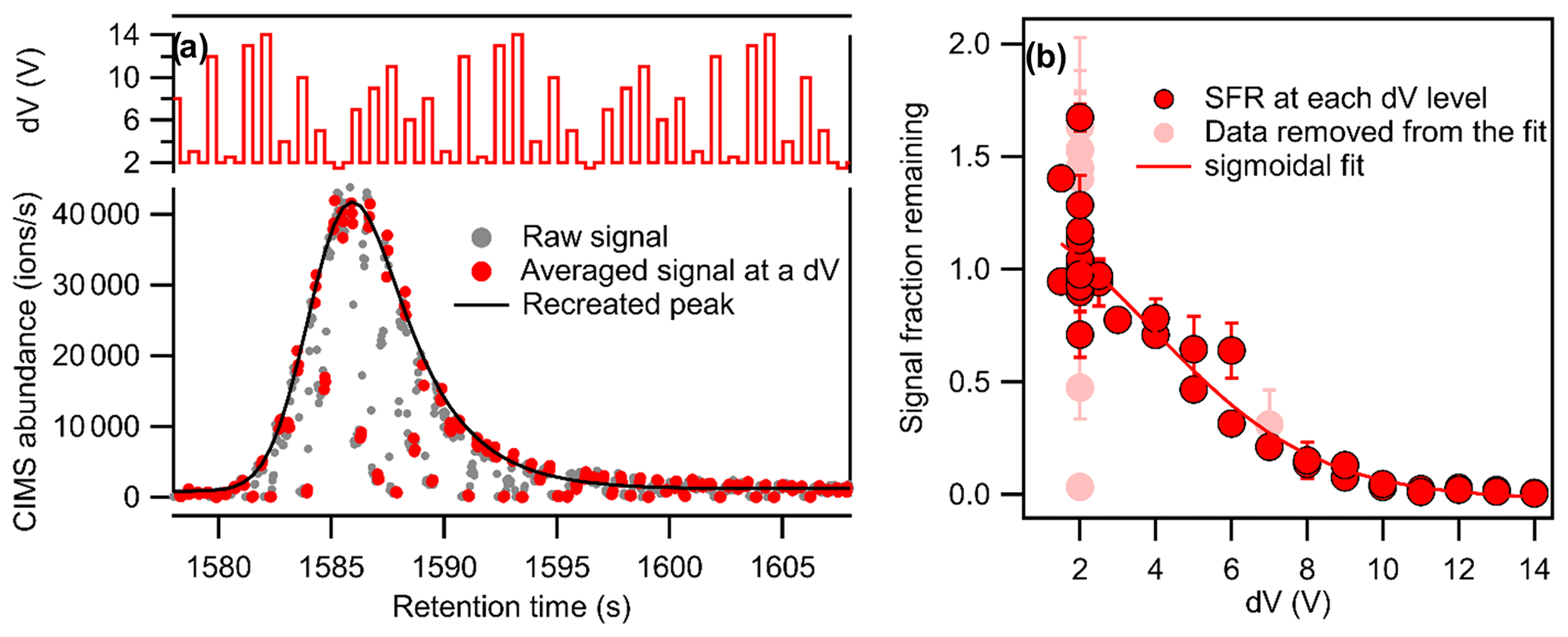
Figure 1Demonstration of the voltage scan method to the GC-CIMS with (a) recreation of the chromatographic peak (grey dots represent all data collected at 20 Hz, while the larger red dots represent the last three data points at each dV level, which are used to calculate the signal at the given dV level) and (b) signal fraction remaining at each voltage difference (dV). Data points in light red, excluded from the sigmoidal fit, are signals from each dV level that do not meet quality control metrics.
The voltage settings of the CIMS in the regular mode are used as a set of baseline values (designated as dV=2 V): fourteen different sets of voltage settings, each of which has a constant voltage deviation from the baseline values (−0.5 to +12 V). The voltage setting is varied at 2.5 Hz, alternating between the baseline values and a set of voltages representing a different dV level. The voltages upstream of the second quadrupole moved simultaneously with the change in dV to maintain a constant electric field gradient across the quadruples and consequently minimize impacts on ion transmission efficiency (Lopez-Hilfiker et al., 2016). As shown in the upper plot of Fig. 1a, the set of dV levels is always in the same order but is not monotonic, randomized to avoid the influence of potential memory effects on the results. An example of the output data for a signal chromatographic peak is shown in Fig. 1a. Grey dots represent all data collected at 20 Hz, while the larger red dots represent the last three spectra at each dV level, which are used to calculate the signal at that voltage scan with the given dV level. The signal fraction remaining (SFR) is calculated as the measured signal, S, at a certain voltage scan, n, of a given dV level, divided by the expected signal, S′, that would have been observed at that scan using baseline voltages, base (here, dV=2 V):
With direct air sampling, the signal changes sufficiently slowly that the baseline signal at a given dV level can be inferred from subsequent and following measurements at the baseline voltages, i.e., . However, in a chromatographic application, the signal varies so rapidly due to the rise and fall of chromatographic peaks that such an approximation is not necessarily reliable. Instead, the changes in the voltage settings back and forth between the baseline condition and a certain voltage difference allow us to recreate the chromatographic peaks for sample runs in the voltage scan mode. As shown in Fig. 1a, the signals obtained with the voltage setting at the baseline condition are used to recreate the chromatographic peak by fitting these points with an exponentially modified Gaussian peak, recreating the peak shown in black in the example. The signal fraction remaining at each voltage level is calculated as the ratio of the observed signal to the recreated peak at the same time.
An example of the obtained signal fraction remaining at different voltage differences is shown in Fig. 1b. The dV50 of the compound can be obtained by fitting the data with a sigmoidal function. Due to the fast acquisition and voltage-scanning rate, some additional quality control metrics are necessary. Specifically, we reject data from a given voltage level if the relative standard deviation of the three included spectra is larger than 20 %, indicating the voltage or signal level is not stable. Additionally, we observe that the set-point voltages are not always reached as expected, so we use the reagent ion signal (which also changes with dV) to evaluate whether or not a given voltage level represents the target dV setting. Specifically, the medians of reagent ion signals at each dV throughout a run cycle are used as standard values of reagent signals per dV, and data are rejected if their corresponding reagent signals are more than 15 % away from the standard value, indicating the target dV setting was not reached. Signals from each dV level that do not meet these quality control metrics (i.e., those in light red in Fig. 1b) are not included in the sigmoidal fit. The dV50 of each compound was calculated from duplicate samples and was excluded from analysis if found to differ by more than 50 %.
2.2 Experimental setup
The TAG-CIMS/FID is used to quantify SOA generated through gas-phase O3 and/or multiple levels of OH oxidation of limonene (Sigma Aldrich, 97 % purity) and 1,3,5-trimethylbenzene (TMB) (Sigma Aldrich, 98 % purity) in a potential aerosol mass (PAM) oxidation flow reactor (OFR) (Lambe et al., 2011). For the convenience of the discussions later, a given set of oxidation experiments is discussed as a “precursor-oxidant” (e.g., limonene-O3).
Experiments were conducted at 25 ∘C, 40 %–50 % relative humidity, and a constant gas flow rate of 12 L min−1 through the OFR. Limonene or TMB was injected into a carrier gas of synthetic air through use of an automated syringe pump at liquid flow rates ranging from 0.95 to 1.9 µL h−1 or corresponding mixing ratios of 236–472 ppbv. During ozonolysis experiments, 35 ppmv O3 was injected at the OFR inlet. During photooxidation experiments, OH and HO2 were generated via O2+H2O photolysis at 254 and 185 nm; over the range of conditions that were used, the estimated OH exposures in the OFR were in the range of (4×10¹⁰–7×10¹¹) (Rowe et al., 2020).
Between sampling from the flow reactor, liquid standards were introduced into the sample collection cell using the automated liquid standard injector on the TAG. Standards analyzed included 1,12-dodecanediol (Sigma Aldrich, 99 % purity), vanillin (Sigma Aldrich, 99 % purity), undecanoic acid (AccuStandard, 100 % purity), hexadecanoic acid (AccuStandard, 100 % purity), levoglucosan (Sigma Aldrich, 99 % purity), and an n-alkanes mixture (C10–C40, AccuStandard, 50 µg mL−1).
2.3 Data analysis
CIMS and FID chromatograms are collected as individual files in each GC run cycle. For each cycle, elemental formulas are identified through the high-resolution fitting of peaks in the mass spectra using the Tofware (Tofwerk, AG and Aerodyne Research, Inc., version 3.1.2) toolkit developed for the IGOR Pro 7 analysis software package (Wavemetrics, Inc.). The chromatograms (i.e., time-series data) of identified formulas in CIMS as well as the FID chromatograms are then imported into TERN, the freely available (https://sites.google.com/site/terninigor/, last access: 26 May 2021) Igor-based software tool for the quantification of chromatographic data (Isaacman-VanWertz et al., 2017), with custom modifications to analyze voltage-scanning data. Integration of CIMS peaks yields units of CIMS-response × s, where CIMS response is ions s−1 (i.e., counts per second, “cps”) normalized to the number of reagent ions (typically in millions). CIMS peak areas are therefore in the units of (ions per million reagent ions) s−1 × s = ions per million reagent ions. Normalization to the reagent ion was not used for generating voltage-scanning curves, following the published approach (Lopez-Hilfiker et al., 2016).
Quantification by FID. Analytes are quantified by integrating chromatographic peaks detected by the FID. Sensitivity of the FID to an oxygenated organic compound is estimated based on its elemental formula, identified by the CIMS, as described by Hurley et al. (2020). In brief, FID detection of hydrocarbons provides a near-universal response per unit carbon mass, which is easily obtained by a multi-point calibration to a hydrocarbon. The average response to carbon in oxygenates decreases proportionally to the oxygen-to-carbon ratio () of the compound. Though the exact decrease in response is driven by the chemical functional groups present, Hurley and co-workers have shown that per-carbon FID sensitivity can be estimated from to within approximately 20 % uncertainty for an individual analyte. We therefore calculate the mass or number of moles of an analyte from its FID peak area based on a calibration response factor to n-alkanes, with a correction for oxygenation based on the elemental formula identified by CIMS (specifically, the FID response per carbon atom relative to n-alkanes , where is the oxygen-to-carbon ratio in the target analyte, Hurley et al., 2020). The sensitivity of an analyte in CIMS, ions generated per mole introduced per million reagent ions, can be determined by dividing its CIMS peak area (ions per million reagent ions) by the number of moles calculated based on the FID peak, yielding units of ions per mole per million reagent ions. Due to the peak integration, this unit is atypical in the CIMS scientific community. Therefore, we also provide a conversion of this unit to the more common metric of CIMS sensitivity, cps per ppt per million reagent ions, based on a specific CIMS operating condition (i.e., 100 mbar in IMR, a 2 slpm sample flow rate, and a 2 slpm reagent ion flow rate). The detailed method of unit conversion is described in the Supplement but essentially involves a conversion by the number of moles entering the instrument per time for a given ppt and flow rate. In the analyses presented here, the sensitivity of an analyte is calculated in three different samples to avoid potential artifacts from data analysis; these three samples represent triplicate samples for the limonene-O3 experiment and three different OH oxidation levels for the precursor-OH experiments. To avoid potential errors introduced by poor chromatographic resolution, low signal, or other issues, we exclude from the analysis any analytes for which the sensitivity calculated from the three samples have a relative standard deviation greater than 50 %. It is critical to note that, because the FID is a single-channel detector, quantification by FID is only possible for peaks that are sufficiently well resolved to be confidently integrated and is not available for every peak observed by CIMS.
Since the determination of analyte sensitivities relies on both CIMS and FID peak area, it is crucial to make sure that the peaks of analyte from CIMS and FID are correctly aligned. To align peaks of the same compounds between CIMS and FID in chromatograms, retention times are corrected based on the linear regression of retention times of internal standards (i.e., vanillin and 1,12-dodecandiol) as well as the two largest peaks. We reject compounds that have differences in peak retention time between CIMS and FID more than 2 s after the retention time correction. We also reject compounds that have significant differences in peak shapes between CIMS and FID.
Instrument blank runs (i.e., runs without sample collection and liquid standard injections) are conducted prior to each oxidation experiment to make sure that there are no visible chromatographic peaks that can interfere with the data analysis later. Blank runs are also tested every five sample runs to check for carry-over or residuals of compounds within the instrument and that no carry-overs of analytes are detected. Additionally, triplicate sample runs are conducted to test for the stability and repeatability of the TAG-CIMS/FID. The results suggest that the relative standard deviations of signals in triplicate runs are within 15 % for CIMS and FID.
3.1 Variability in isomer sensitivity
As an example of the data, Fig. 2b shows the chromatograms of the ion (C9H14O4)I− from a sample of aerosol collected in the limonene-OH experiment. The FID abundance (y axis of Fig. 2a is a single-channel signal of total ions produced by the mass of carbon combusted; Holm, 1999), so each analyte (i.e., chromatographic peak eluting at a given retention time), responds with similar mass-based sensitivity. Co-eluting peaks are not well resolved and may not be able to be accurately integrated, as there is no additional dimension of separation (e.g., mass spectra) to improve resolution beyond what is shown. In contrast, CIMS signals include separation by mass of detected ions, so co-eluting analytes of different elemental formulas can be easily resolved. The chromatogram displayed, Fig. 2b, is the normalized ion count signals of a single ion, (C9H14O4)I−. Five isomers, highlighted with numbers in Fig. 2b, were able to be matched to FID peaks to calculate sensitivities with relative standard deviations less than 50 %. While larger peaks can be easily correlated between the FID and CIMS by retention time, compounds with small peak areas such as Compounds 3 and 4 in Fig. 2b are also correlated when their peak shapes between FID and CIMS are similar and they have comparable behavior across different oxidation levels to ensure the proper peak assignment. As an example, Fig. S1 in the Supplement shows the peaks representing Compounds 3 and 4, which have the same retention time and peak shape in the CIMS and FID and follow the similar trends with the change in OH exposure levels.

Figure 2An example of isomers quantified in (b) the chromatogram of ion (C9H14O4)I− in CIMS with (a) their corresponding FID peaks (highlighted in red). The peaks marked with numbers are those included in the analysis of isomer sensitivity.
Given that the FID sensitivity of oxygenated organics is primarily a function of carbon and oxygen content (to within ∼20 %) (Hurley et al., 2020) and that these isomers all have the same elemental formula, FID peak areas (highlighted in red in Fig. 2a) are proportional to the number of moles of those compounds. Differences in sensitivity are qualitatively clear: for example, Compounds 2 and 3 have a relatively similar number of moles in the sample (i.e., similar FID areas) yet show at least 1 order of magnitude difference in CIMS response. The CIMS sensitivities of the five compounds can be quantified as discussed and are found to span the range from 3.1×10¹⁶ ions per mole per million reagent ions (Compound 1) to 6.5×10¹⁴ ions per mole per million reagent ions (Compound 3). The 2 orders of magnitude range of sensitivities of the five identified isomers shows that, while sharing the same elemental formula, isomers may have significantly different CIMS sensitivities. These differences may result in biases during quantification when using a direct-air-sampling CIMS without GC pre-separation that provides resolution of isomers.
Notably, although this instrument TAG-CIMS/FID is specifically configured to collect only particle-phase samples, this calibration technique for quantifying CIMS sensitivity could be applied to gas-phase samples using a different instrument configuration and should be applicable to any GC-based instrument employed upstream of the two detectors as long as the analyte can be collected by the upstream instrument, separated by the GC column, and transferred to both detectors. Additionally, the coupled TAG-CIMS/FID can be applied to investigate the change in isomer composition with the increase in OH levels in future studies. It is possible that the isomers of a formula produced at higher OH levels are more oxidized compounds, thus changing the isomer distributions in the formula. In this case, the average sensitivity of the formula will likely increase at higher OH levels.
Calibration of CIMS using FID requires the target analyte to be detected by both detectors and to have a well-resolved chromatographic peak in FID. For example, there are certainly other isomers (i.e., chromatographic peaks) in Fig. 2b besides the highlighted five ones. However, some of those isomers are not included in the discussion because no FID peaks or well-resolved FID peaks are present at the same retention time as their CIMS peaks. Conversely, it is possible that some of the FID peaks are isomers of this formula that are not detectable by CIMS. Due to the higher chemical resolution of the CIMS, the number of isomers available for intercomparison is primarily limited by the chromatographic resolution of the FID since FID is a single-channel detector. This limitation can be mitigated by collecting data under a wide range of conditions or environments. Once the CIMS sensitivity of a compound is obtained, quantification can be achieved for those compounds in other poor-signal conditions or even without the coupling of the FID.
Additionally, the use of a GC column, which is selective towards a certain range of volatility and polarity of compounds, limits the detection to specific ranges of compounds and/or could induce thermal decomposition of some sampled compounds to form analytes not present in the original sample (Isaacman-VanWertz et al., 2016). Nevertheless, quantification of individual analytes can be critical for understanding source and chemical pathways (Nozière et al., 2015) and can provide fundamental insight into the capabilities and limitations of a given ion reagent chemistry. Furthermore, while decomposition during analysis may impact the scientific interpretation of the collected sample, decomposition is expected to primarily occur during desorption or GC analysis and is therefore upstream of the detectors; both detectors consequently “see” the same analyte whether or not decomposition occurs, and it does not impact measurements of CIMS sensitivity of the molecules that do reach the detectors. It is well established that sensitivity is humidity dependent for many chemicals in an iodide CIMS (Lee et al., 2014). Because analytes entering the IMR come from the GC in a dry helium flow, the relative humidity in the IMR is stable and can be controlled by adjusting the mixed water vapor in the reagent ion flow. Therefore, the coupled TAG-CIMS/FID provides opportunities for future work to quantitatively investigate the humidity dependency of sensitivity of those chemicals.
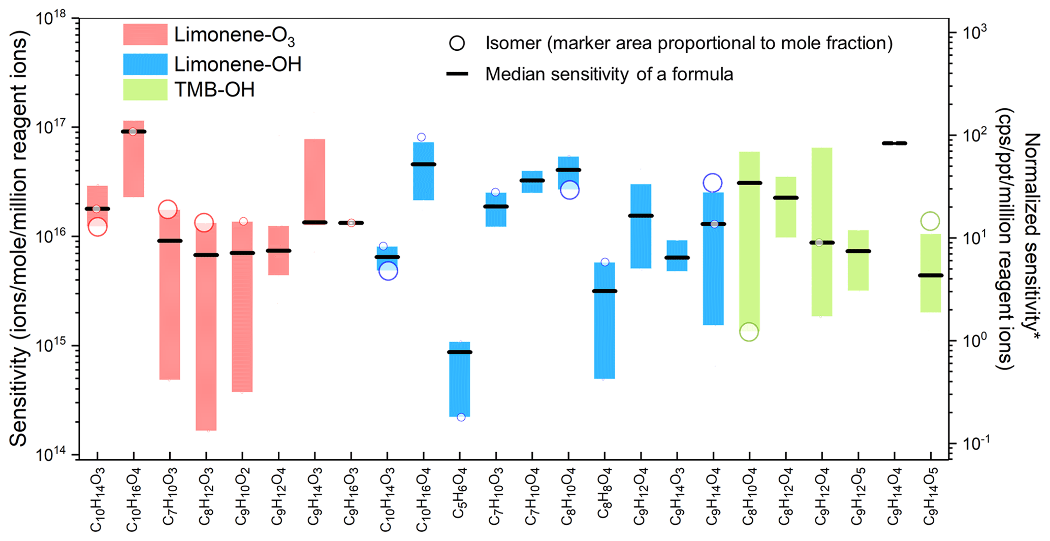
Figure 3Sensitivities of constituent isomers of formulas for which at least two isomers had sensitivities obtained in the oxidation experiments. Each circle shows the sensitivity of an isomer, and the area of the circle represents the mole fraction of the isomer in the formula. Boxes represent the first to third quartiles. Black lines are the median values of the sensitivities. *: unit converted for direct-air-sampling CIMS using 100 mbar in IMR, 2 slpm sample flow rate, and 2 slpm reagent ion flow rate.
To systematically study the variance of isomer sensitivity, formulas with multiple isomers identified in the oxidation experiments are summarized in Fig. 3 (as noted above, only isomers with sensitivities with less than 50 % relative standard deviation in three samples are included). The results suggest that the sensitivity of isomers typically vary by 1 order of magnitude, with a maximum deviation of 2 orders of magnitude, for instance, in the case of (C8H12O3)I− in limonene-O3, (C9H14O4)I− in limonene-OH (also shown in Fig. 2), and (C9H12O4)I− in TMB-OH. In a minority of cases, sensitivities vary by only a factor of 2 to 4 (e.g., (C9H16O3)I− in limonene-O3, (C10H14O3)I− in limonene-OH, and (C9H14O4)I− in TMB-OH). Notably, molecules of the same formula produced through two different chemistries (e.g., (C9H14O4)I− in limonene-OH and TMB-OH) also differ to approximately the same degree, supporting the conclusion that a measured formula may consist of a different set of isomers depending on the sampling environment. The significant variance of isomer sensitivity indicates that if a CIMS with direct air sampling is used, the concentration of a given formula may be significantly biased towards the concentration of the most sensitive isomer within the formula, while other isomers, which could actually be more abundant on a per-mole basis, may be overwhelmed. As an example, consider (C8H12O3)I− in the limonene-O3 experiment, which includes a low-sensitivity, high-concentration isomer and a high-sensitivity, low-concentration isomer. The low-concentration isomer is approximately 80× more sensitive but 5× less abundant (represented by the ratio of the marker area in Fig. 3) than the high-concentration isomer. In this example, ∼95 % of the CIMS signal is from an isomer that accounts for less than 20 % of the mass, which could introduce biases in data interpretation (if, for instance, the two isomers can come from different sources or represented different chemistries). The example demonstrates that isomer resolution, achieved by coupling a CIMS with a GC and a FID, consequently provides not only additional detail about a sample, but is also critical for the quantification of less sensitive isomers.
3.2 Prediction of sensitivity using dV50
Previous work has shown a log-linear relationship between sensitivity and dV50. However, these relationships were established based on only a limited number of chemical standards, mostly mono- and di-acids (Brophy and Farmer, 2016; Iyer et al., 2016; Lopez-Hilfiker et al., 2016), and demonstrate significant scatter around the trend. In this work, the quantification of compounds based on FID response allows us to broaden the investigation of this relationship from liquid standards to oxidation products. Of all observed analytes, sensitivities calculated for a total of 63 oxidation products and 3 liquid chemical standards passed all the data quality checks for inclusion in this analysis (i.e., sufficient FID resolution for quantification, relative standard deviations of sensitivity less than 50 % for triplicate (limonene-O3) or three different OH level measurements, relative standard deviations of dV50 less than 50 % for duplicate measurements). The calculated sensitivities of all 66 compounds and their dV50 obtained using the voltage scan method are plotted in Fig. 4. Sensitivities of analytes included in the discussion vary across 3 orders of magnitude. A plateau of sensitivity, which is an indication of maximum sensitivity, is observed for compounds with dV greater than 7 V. Levoglucosan, which is known to be detected at the collision limit (Lopez-Hilfiker et al., 2016), is one of the compounds that nearly reach the maximum sensitivity in this study. The finding agrees with those reported in the literature that the maximum sensitivity can be reached if the iodide–molecule reaction is only limited by the formation rate (i.e., collision limit) (Huey et al., 1995).
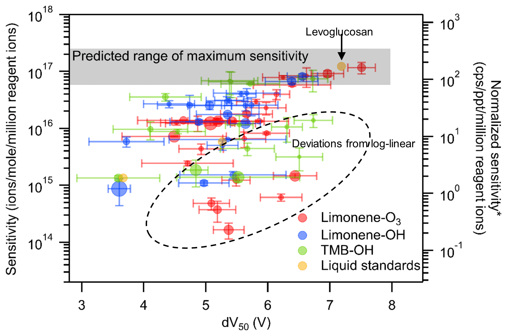
Figure 4Relationship between sensitivities and dV50 of compounds identified in oxidation experiments as well as liquid standards. Each data point is a compound identified with the marker area representing the moles of the compound. The error bars on the y axis are the standard deviation of sensitivity in triplicate (limonene-O3) or three different OH level measurements (limonene-OH and TMB-OH). The error bars on the x axis are the standard deviation of dV50 in duplicate measurements. *: unit converted for direct-air-sampling CIMS using 100 mbar in IMR, 2 slpm sample flow rate, and 2 slpm reagent ion flow rate.
The observed plateau of sensitivity is in the range expected for maximum sensitivity (calculated in the Supplement) based on instrument operating conditions; the colored grey bar in Fig. 4 spans the range from the calculated kinetic-limited maximum sensitivity to 4 times lower values (observed by Isaacman-VanWertz et al. (2018) to be the maximum sensitivity using an instrument of the same design as that used here). The right axis provides a direct mathematical conversion between the left axis and more typical CIMS units assuming a sample flow of 2 slpm (as opposed to the 0.7 sccm used here). It provides a general context for the conversion between the units but is not fully representative of the conversion due to differences in flow between our setup and typical operation and its concomitant impacts on the residence time within the reaction region. While the detailed analysis is in the Supplement, true maximum sensitivity under our IMR conditions but with typical flows is found to be 88 cps per ppt per million reagent ions (not 350 as implied in Fig. 4). For this large set of individual analytes, the relationship between sensitivity and dV50 shown by Iyer et al. (2016) and Lopez-Hilfiker et al. (2016) is not so clear. A log-linear relationship defines an apparent upper bound of sensitivity, but approximately one-quarter of compounds (dashed region) have sensitivities substantially lower than this relationship. These results suggest that, for calibrating individual components, the log-linear relationship between sensitivity and dV50 may provide some rough indications of sensitivity but is fairly imprecise.
The data shown in Fig. 4 are inherently different than the data from a typical, direct-air-sampling application of CIMS in ways that could impact the application of the relationship between sensitivity and dV50. Direct-air-sampling CIMS classifies analytes on an elemental formula basis, while a TAG-CIMS can differentiate isomers and provide quantification down to the isomer resolution. The analytes significantly deviating from the log-linear relationship are mostly less sensitive compounds. For CIMS with direct air sampling, the responses of the less sensitive isomers might be overwhelmed by the signals of more sensitive isomers of the same formula. Such an outcome would potentially strengthen the observed log-linear relationship but would underestimate the observed mass of that compound (and consequently formula). To examine the applicability of the voltage scan method to CIMS operated with direct air sampling, we convolute resolved isomers into their elemental formulas. The sensitivity of a formula is calculated as the average of isomer sensitivities weighted by their number of moles, while the dV50 of a formula is calculated as the average of dV50 weighted by their CIMS abundance (i.e., chromatographic peak area in CIMS data). Note that the signal-weighted method to calculate formula-based dV50 is found to yield reasonable approximations of the true dV50, and the detailed discussions are in the Supplement. The result of averaging and weighting each parameter in these ways recreates how that formula would respond in direct-air-sampling CIMS if it had the same isomer composition; we note that a direct comparison cannot be made by a simple direct air sample of the same mixture due to artifacts introduced by the GC (both positive – the formation of new compounds through thermal decomposition – and negative – the inability to elute highly polar compounds). To ensure averaged formulas are a reasonable representation of a hypothetical direct-air CIMS sample, formulas are removed from the analysis if (1) the formula has only two isomers and one of the isomers does not have a calculated sensitivity and/or (2) the isomer with the most abundant CIMS signal does not have a reported sensitivity. The resulting relationship between sensitivity and dV50 on a per-formula basis can be plotted (Fig. 5). The compounds that are filtered by these criteria are not statistically significantly different from the compounds that pass these criteria (one-way analysis of variance – ANOVA – test, p=0.36, and 0.71 for log-transformed sensitivity and dV50, respectively).
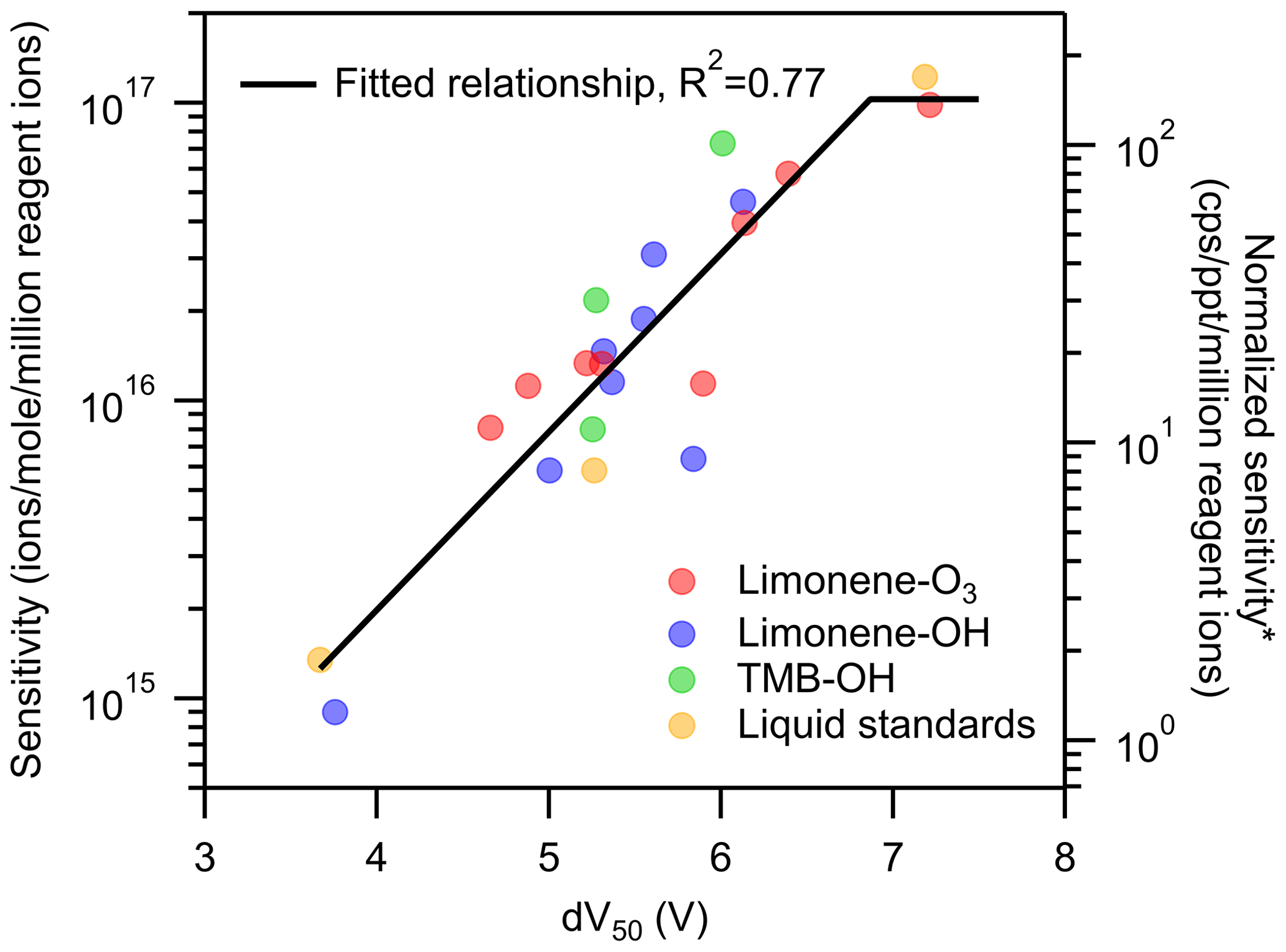
Figure 5Sensitivity vs. dV50 on a per-formula basis with a linear regression on the formulas. *: unit converted for direct-air-sampling CIMS using 100 mbar in IMR, a 2 slpm sample flow rate, and a 2 slpm reagent ion flow rate.
As shown in Fig. 5, the log-linear relationship improves when considered on a per-formula basis, though significant scatter remains. Linear regression for formulas of dV50<7 V (i.e., having lower than maximum sensitivity) has a reasonable correlation (R2=0.77), with a decrease of 0.6 log units (i.e., a factor of 100.6) of sensitivity per volt change in dV50. This slope is similar to, but slightly shallower than, the slope observed in previous work of 0.9 log units per volt (Lopez-Hilfiker et al., 2016).
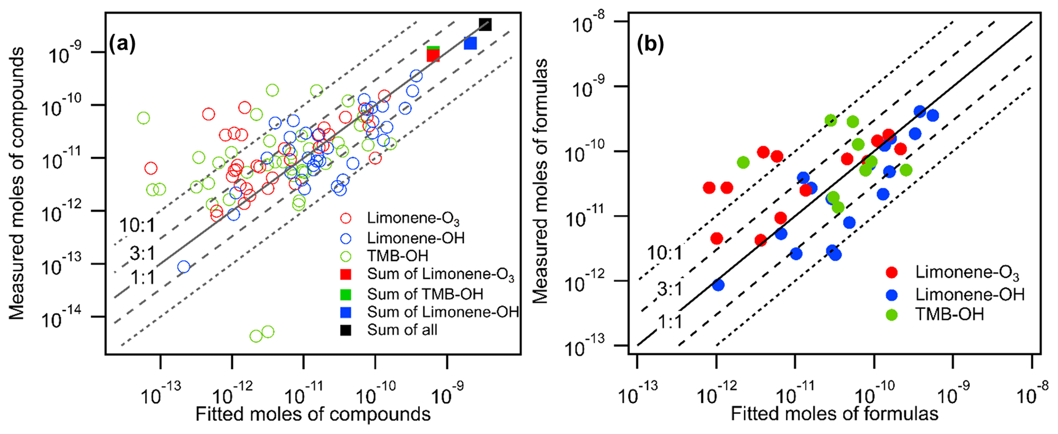
Figure 6Measured moles of (a) compounds and (b) formulas (i.e., summation of isomers within each formula) in all oxidation experiments vs. their fitted moles using the linear regression equation obtained in Fig. 5.
The goal of the voltage scan calibration approach is to predict the sensitivities of analytes without conducting individual calibrations with chemical standards in permeation tubes. To quantify the error introduced in this approach, we use the fitted linear regression equation in Fig. 5 to calculate a sensitivity for each compound based on its observed dV50. As described by Bi et al. (2021a), sensitivity predicted in the log-linear-based calibration method is inherently biased, and the bias can be corrected based on residual scatter around the nominal relationship, ; given that the calculated of a residual is 0.22, predicted sensitivities are expected to by biased low by a factor of 1.14 and so are adjusted by that factor here. In Fig. 6a, the moles of each compound calculated using the fit from their dV50 (“fitted moles”) are compared to the measured moles calculated using the FID data. Compounds that were filtered out of Fig. 5 using the criteria described above are included in the results shown in Fig. 6. By including compounds not used to generate the linear relationship, this approach therefore provides a more realistic and conservative evaluation of the approach. The results show that about 60 % and 80 % of compounds are estimated within factor of 3 and 10 uncertainties, respectively, indicating that the voltage scan approach has high uncertainties for individual components. The uncertainty for individual compounds found in this work is similar to the studies originally proposing this log-linear relationship (i.e., 77 % and 85 % of compounds are estimated within factor of 3 and 10 uncertainties, respectively) (Iyer et al., 2016). The uncertainty is likely caused by the transfer of uncertainty from the empirical correlation itself and the consideration of a wider range of chemical species. It is also possible that optimizing certain instrumental parameters could improve the accuracy of the voltage-scanning method, but future work is needed to investigate the optimization method further. Additionally, to examine the accuracy of the predictions for a direct-air-sampling CIMS, we compare the fitted moles with the measured moles on a per-formula basis (i.e., the summation of moles of isomers within each formula) in Fig. 6b. Most of the formulas are estimated within factor of 3 uncertainties. Notably, a factor of 3 is in approximate agreement with the uncertainty previously estimated for individual components quantified by iodide CIMS voltage scanning (Isaacman-VanWertz et al., 2018).
Because the log-linear relationship of voltage scanning provides a reasonable central tendency, its application does not introduce significant bias for quantifying the summation of a class of compounds. The predicted total moles of compounds measured agree well with the measured total moles (shown as rectangular markers in Fig. 6a, with errors within 30 % within an oxidation system and for all oxidation systems combined), although predicted moles of individual compounds have relatively high errors. The finding agrees with earlier statistical analysis suggesting that the summation of multiple analytes with high scatters of sensitivity around a nominal relationship can reduce uncertainty (Bi et al., 2021a) and is in qualitative agreement with the finding by Isaacman-VanWertz et al. (2018) that uncertainty in the sum of ions was substantially lower than uncertainty in an individual analyte. We conclude that, although using voltage scanning introduces high error into the estimation of sensitivity for individual compounds, the approach provides a reasonable estimate of the summed abundance.
3.3 Implications of the retention time index
The use of a GC expands the data with another dimension, retention time, which is generally governed by the polarity and vapor pressure of the compound and could potentially provide additional information to inform estimation of CIMS sensitivity. Since a GC column with a polar stationary phase is used in the TAG-CIMS/FID, we expect the compound with high polarity and/or low vapor pressure to have longer retention time in the chromatogram. Polarity and vapor pressure are not fully independent: the presence of polar functional groups (e.g., hydroxyl and carboxyl groups) tends to accompany larger decreases in vapor pressure than less polar groups (e.g., carbonyl groups) (Kroll and Seinfeld, 2008). Retention time is therefore expected to also positively correlate with iodide CIMS sensitivity, which generally increases with the presence of polar functional groups (Lee et al., 2014). To examine the hypothesis, we plot the relationship between sensitivity and retention index for compounds identified in oxidation experiments in Fig. 7 (retention index = retention time of an analyte adjusted such that n-alkanes are defined to elute at spacings of 100 units; Onuska and Karasek, 1984). The results suggest that there is a qualitative linear trend between log(sensitivity) and retention time index, particularly for analytes with higher abundances. Binning the data into equally distributed groups (octiles) reveals the tendency for later retention times to accompany higher sensitivity. Specifically, the latest eluting two bins are more sensitive than the earliest eluting two bins with statistical significance of p<0.05 using a Wilcoxon signed-rank test; differences between intermediate bins are not statistically significant. A major driver of retention time is molecule size (e.g., number of carbon atoms), which does not necessarily impact iodide CIMS sensitivity. Consequently, the coarseness and scatter of the relationship between retention time and iodide CIMS sensitivity may be due to the concurrent impacts on retention time of polarity and vapor pressure.
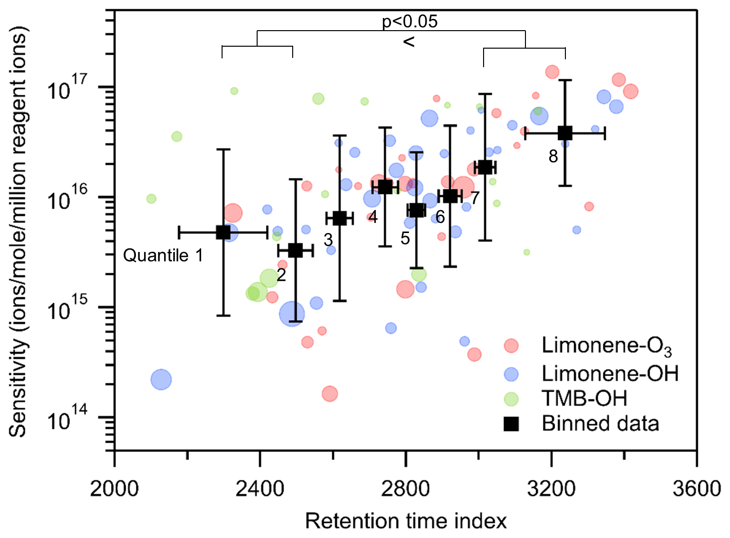
Figure 7Relationship between sensitivities and retention time index of all compounds in oxidation experiments. Black markers are all data equally divided into eight bins based on the ranking of their sensitivity and retention time index, centered on averages with error bars representing the standard deviation of sensitivity and retention time index. The size of the round marker represents the number of moles of each compound.
To better isolate the effects of polarity in the relationship between retention time and vapor pressure, we attempt to constrain molecule size. By examining differences between retention times of compounds with a given elemental formula, the effects of molecular structure and differences in chemical functionality can be separated from some of the features that impact vapor pressure (number of carbon atoms, molecular weight, etc.). If two isomers have a similar chemical structure and functional group, their retention time should be relatively close due to the minor differences in vapor pressure and polarity, and their iodide CIMS sensitivity is likely to be roughly similar. Conversely, an isomer with a higher retention time index is expected to contain more polar functional groups, which are also expected to have a large impact on vapor pressure. To test this hypothesis, we compare the sensitivities and retention index of all isomer pairs (i.e., for a formula of n isomers, there are unique isomer pairs). For each isomer pair, we calculate the difference between the log(sensitivity) of the later- vs. earlier-eluting isomers and compare it to their difference in retention index, shown in Fig. 8. Eight equally distributed bins (octiles) are included in Fig. 8 to better identify trends and allow statistical comparisons. Qualitatively, it is apparent that isomers with small differences in retention time vary widely in their sensitivities, frequently differing by 1 order of magnitude, while later-eluting isomers tend to have higher sensitivities. Isomers that elute substantially later (octiles 5–8) have statistically higher sensitivities by, on average, roughly half an order of magnitude (a factor of 3 to 4). Conversely, there is no statistical difference in the sensitivities of isomers with retention indices within ∼300 of each other (octiles 1–4). In other words, while iodide CIMS sensitivity of isomers with similar retention times is not a strong function of retention time, later elution does indicate some tendency for higher sensitivity, presumably driven by the presence of higher-polarity functional groups.
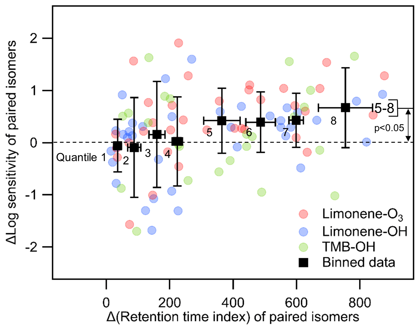
Figure 8The relationship between differences (Δ) in log(sensitivity) and retention index for all pairs of isomers with a given formula. Black markers are all data equally divided into eight bins (octiles) centered on averages with error bars representing standard deviations.
While the analysis here does not provide a sufficiently deep understanding of the relationship between sensitivity and column retention to produce a quantitative approach for estimating sensitivity, it does demonstrate an approach by which interactions with the GC column can provide insight into iodide CIMS sensitivity. These data suggest that the properties of a molecule that drive iodide CIMS sensitivity are correlated, but not tightly, with the properties that drive the retention time of this particular GC stationary phase. Future detailed studies and physicochemical modeling of the column retention of analytes could make use of these relationships to better understand the factors driving sensitivity and selectivity of a given CIMS reagent ion chemistry.
By coupling a TAG simultaneously to a FID and an iodide CIMS, we quantify isomer-resolved CIMS sensitivity (i.e., CIMS signal divided by the number of moles of analytes quantified using FID signal) for liquid standards as well as oxidation products for which commercial chemical standards are not available. The variance of isomer sensitivities for oxidation products in an iodide CIMS is found to be generally 1 order of magnitude and up to 2 orders of magnitude. The wide range of isomer sensitivities indicates that if an iodide CIMS with direct air sampling is used, measurements of formulas are likely to minimize the contributions of certain (likely less polar) isomers. The concentration of a given formula would be expected to be biased towards the concentration of the most sensitive isomer within the formula, even in cases where this isomer is not the most abundant.
We then investigate the previously reported log-linear calibration relationship between iodide CIMS sensitivity and dV50 by applying the relationship to a broader range of chemicals including oxidation products. We find that estimating sensitivity of a given compound from its declustering voltage (i.e., dV50) carries high uncertainties (0.5 to 1 order of magnitude). However, the voltage scan approach to calibration can be used to estimate aggregate/summed moles of all analytes with low error (∼30 % differences between predicted and measured moles) since summing multiple analytes statistically reduced the uncertainty in the sum (Bi et al., 2021a). These results imply that in the interpretation of direct-air-sampling CIMS data, quantification based on declustering voltage is highly uncertain for individual compounds and relatively uncertain for individual formulas. Nevertheless, a nominal voltage-scanning relationship built using elemental formulas represents a central tendency and can be used to estimate total mass or moles reasonably well.
We further find that the additional dimension of GC retention time provides some possible advantages to understand iodide CIMS sensitivity. There exists a positive relationship between retention time in the GC column and iodide CIMS sensitivity, but the relationship is not yet sufficiently well understood to become quantitatively useful. Future work is needed to investigate the relationship between GC retention time and iodide CIMS sensitivity.
All raw and processed data collected as part of this project are available upon request, which can be sent to Chenyang Bi (chenyangbi@vt.edu) or Gabriel Isaacman-VanWertz (ivw@vt.edu).
The supplement related to this article is available online at: https://doi.org/10.5194/amt-14-6835-2021-supplement.
CB led the instrumentation design, experimental setup, and consequent data analysis under the guidance of GIVW. GIVW, JEK, BML, and MRC contributed to the development of the theory of the described approach. GIVW, GOF, JEK, JTJ, and DRW contributed to hardware design and instrumentation. JEK, WX, ATL, and MSC contributed to data collection and analysis. CB prepared the manuscript with contributions from all the authors.
Jordan E. Krechmer, Megan S. Claflin, Wen Xu, Andrew T. Lambe, John T. Jayne, Douglas R. Worsnop, Brian M. Lerner, and Manjula R. Canagaratna are employed by Aerodyne Research, Inc., which commercializes TAG and CIMS instruments for geoscience research.
Publisher's note: Copernicus Publications remains neutral with regard to jurisdictional claims in published maps and institutional affiliations.
We would like to thank the Alfred P. Sloan Foundation Chemistry of the Indoor Environment Program for supporting this work.
This research has been supported by the Alfred P. Sloan Foundation (grant no. P-2018-11129).
This paper was edited by Bin Yuan and reviewed by two anonymous referees.
Aljawhary, D., Lee, A. K. Y., and Abbatt, J. P. D.: High-resolution chemical ionization mass spectrometry (ToF-CIMS): application to study SOA composition and processing, Atmos. Meas. Tech., 6, 3211–3224, https://doi.org/10.5194/amt-6-3211-2013, 2013.
Arangio, A. M., Tong, H., Socorro, J., Pöschl, U., and Shiraiwa, M.: Quantification of environmentally persistent free radicals and reactive oxygen species in atmospheric aerosol particles, Atmos. Chem. Phys., 16, 13105–13119, https://doi.org/10.5194/acp-16-13105-2016, 2016.
Atkinson, R.: Atmospheric chemistry of vocs and nox, Atmos. Environ., 34, 2063–2101, https://doi.org/10.1016/S1352-2310(99)00460-4, 2000.
Atkinson, R. and Arey, J.: Atmospheric degradation of volatile organic compounds, Chem. Rev., 103, 4605–4638, https://doi.org/10.1021/cr0206420, 2003.
Bertram, T. H., Kimmel, J. R., Crisp, T. A., Ryder, O. S., Yatavelli, R. L. N., Thornton, J. A., Cubison, M. J., Gonin, M., and Worsnop, D. R.: A field-deployable, chemical ionization time-of-flight mass spectrometer, Atmos. Meas. Tech., 4, 1471–1479, https://doi.org/10.5194/amt-4-1471-2011, 2011.
Bi, C., Krechmer, J. E., Canagaratna, M. R., and Isaacman-VanWertz, G.: Correcting bias in log-linear instrument calibrations in the context of chemical ionization mass spectrometry, Atmos. Meas. Tech., 14, 6551–6560, https://doi.org/10.5194/amt-14-6551-2021, 2021a.
Bi, C., Krechmer, J. E., Frazier, G. O., Xu, W., Lambe, A. T., Claflin, M. S., Lerner, B. M., Jayne, J. T., Worsnop, D. R., Canagaratna, M. R., and Isaacman-VanWertz, G.: Coupling a gas chromatograph simultaneously to a flame ionization detector and chemical ionization mass spectrometer for isomer-resolved measurements of particle-phase organic compounds, Atmos. Meas. Tech., 14, 3895–3907, https://doi.org/10.5194/amt-14-3895-2021, 2021b.
Brophy, P.: Development, characterization, and deployment of a high- resolution time-of-flight chemical ionization mass spectrometer (hr-tof-cims) for the detection of carboxylic acids and trace-gas species in the troposphere, PhD, Colorado State University, Fort Collins, Colorado, USA, 2016.
Brophy, P. and Farmer, D. K.: Clustering, methodology, and mechanistic insights into acetate chemical ionization using high-resolution time-of-flight mass spectrometry, Atmos. Meas. Tech., 9, 3969–3986, https://doi.org/10.5194/amt-9-3969-2016, 2016.
Burnett, R. T., Pope, C. A., Ezzati, M., Olives, C., Lim, S. S., Mehta, S., Shin, H. H., Singh, G., Hubbell, B., Brauer, M., Anderson, H. R., Smith, K. R., Balmes, J. R., Bruce, N. G., Kan, H., Laden, F., Prüss-Ustün, A., Turner, M. C., Gapstur, S. M., Diver, W. R., and Cohen, A.: An integrated risk function for estimating the global burden of disease attributable to ambient fine particulate matter exposure, Environ. Health Persp., 122, 397–403, https://doi.org/10.1289/ehp.1307049, 2014.
Crounse, J. D., McKinney, K. A., Kwan, A. J., and Wennberg, P. O.: Measurement of gas-phase hydroperoxides by chemical ionization mass spectrometry, Anal. Chem., 78, 6726–6732, https://doi.org/10.1021/ac0604235, 2006.
Ditto, J. C., Barnes, E. B., Khare, P., Takeuchi, M., Joo, T., Bui, A. A. T., Lee-Taylor, J., Eris, G., Chen, Y., Aumont, B., Jimenez, J. L., Ng, N. L., Griffin, R. J., and Gentner, D. R.: An omnipresent diversity and variability in the chemical composition of atmospheric functionalized organic aerosol, Commun. Chem., 1, 1–13, https://doi.org/10.1038/s42004-018-0074-3, 2018.
Goldan, P. D., Kuster, W. C., Williams, E., Murphy, P. C., Fehsenfeld, F. C., and Meagher, J.: Nonmethane hydrocarbon and oxy hydrocarbon measurements during the 2002 new england air quality study, J. Geophys. Res.-Atmos., 109, 1–14, https://doi.org/10.1029/2003JD004455, 2004.
Goldstein, A. H. and Galbally, I. E.: Known and unexplored organic constituents in the earth's atmosphere, Environ. Sci. Technol., 41, 1514–1521, https://doi.org/10.1021/es072476p, 2007.
Goldstein, A. H., Daube, B. C., Munger, J. W., and Wofsy, S. C.: Automated in-situ monitoring of atmospheric non-methane hydrocarbon concentrations and gradients, J. Atmos. Chem., 21, 43–59, https://doi.org/10.1007/BF00712437, 1995.
Grob, R. L. and Barry, E. F.: Modern practice of gas chromatography, 4th edition, John Wiley and Sons, Inc., Hoboken, New Jersey, USA, 2004.
Hallquist, M., Wenger, J. C., Baltensperger, U., Rudich, Y., Simpson, D., Claeys, M., Dommen, J., Donahue, N. M., George, C., Goldstein, A. H., Hamilton, J. F., Herrmann, H., Hoffmann, T., Iinuma, Y., Jang, M., Jenkin, M. E., Jimenez, J. L., Kiendler-Scharr, A., Maenhaut, W., McFiggans, G., Mentel, Th. F., Monod, A., Prévôt, A. S. H., Seinfeld, J. H., Surratt, J. D., Szmigielski, R., and Wildt, J.: The formation, properties and impact of secondary organic aerosol: current and emerging issues, Atmos. Chem. Phys., 9, 5155–5236, https://doi.org/10.5194/acp-9-5155-2009, 2009.
Helmig, D., Ortega, J., Duhl, T., Tanner, D., Guenther, A., Harley, P., Wiedinmyer, C., Milford, J., and Sakulyanontvittaya, T.: Sesquiterpene emissions from pine trees – identifications, emission rates and flux estimates for the contiguous united states, Environ. Sci. Technol., 41, 1545–1553, https://doi.org/10.1021/es0618907, 2007.
Holm, T.: Aspects of the mechanism of the flame ionization detector, J. Chromatogr. A, 842, 221–227, https://doi.org/10.1016/S0021-9673(98)00706-7, 1999.
Huey, L. G., Hanson, D. R., and Howard, C. J.: Reactions of sf6- and i- with atmospheric trace gases, J. Phys. Chem., 99, 5001–5008, https://doi.org/10.1021/j100014a021, 1995.
Hurley, J. F., Kreisberg, N. M., Stump, B., Bi, C., Kumar, P., Hering, S. V., Keady, P., and Isaacman-VanWertz, G.: A new approach for measuring the carbon and oxygen content of atmospherically relevant compounds and mixtures, Atmos. Meas. Tech., 13, 4911–4925, https://doi.org/10.5194/amt-13-4911-2020, 2020.
Isaacman-Vanwertz, G., Massoli, P., O'Brien, R., Lim, C., Franklin, J. P., Moss, J. A., Hunter, J. F., Nowak, J. B., Canagaratna, M. R., Misztal, P. K., Arata, C., Roscioli, J. R., Herndon, S. T., Onasch, T. B., Lambe, A. T., Jayne, J. T., Su, L., Knopf, D. A., Goldstein, A. H., Worsnop, D. R., and Kroll, J. H.: Chemical evolution of atmospheric organic carbon over multiple generations of oxidation, Nat. Chem., 10, 462–468, https://doi.org/10.1038/s41557-018-0002-2, 2018.
Isaacman-VanWertz, G., Yee, L. D., Kreisberg, N. M., Wernis, R., Moss, J. A., Hering, S. V., De Sá, S. S., Martin, S. T., Alexander, M. L., Palm, B. B., Hu, W., Campuzano-Jost, P., Day, D. A., Jimenez, J. L., Riva, M., Surratt, J. D., Viegas, J., Manzi, A., Edgerton, E., Baumann, K., Souza, R., Artaxo, P., and Goldstein, A. H.: Ambient gas-particle partitioning of tracers for biogenic oxidation, Environ. Sci. Technol., 50, 9952–9962, https://doi.org/10.1021/acs.est.6b01674, 2016.
Isaacman-VanWertz, G., Sueper, D. T., Aikin, K. C., Lerner, B. M., Gilman, J. B., de Gouw, J. A., Worsnop, D. R., and Goldstein, A. H.: Automated single-ion peak fitting as an efficient approach for analyzing complex chromatographic data, J. Chromatogr. A, 1529, 81–92, https://doi.org/10.1016/j.chroma.2017.11.005, 2017.
Isaacman, G., Kreisberg, N. M., Worton, D. R., Hering, S. V., and Goldstein, A. H.: A versatile and reproducible automatic injection system for liquid standard introduction: application to in-situ calibration, Atmos. Meas. Tech., 4, 1937–1942, https://doi.org/10.5194/amt-4-1937-2011, 2011.
Isaacman, G., Kreisberg, N. M., Yee, L. D., Worton, D. R., Chan, A. W. H., Moss, J. A., Hering, S. V., and Goldstein, A. H.: Online derivatization for hourly measurements of gas- and particle-phase semi-volatile oxygenated organic compounds by thermal desorption aerosol gas chromatography (SV-TAG), Atmos. Meas. Tech., 7, 4417–4429, https://doi.org/10.5194/amt-7-4417-2014, 2014.
Iyer, S., Lopez-Hilfiker, F., Lee, B. H., Thornton, J. A., and Kurtén, T.: Modeling the detection of organic and inorganic compounds using iodide-based chemical ionization, J. Phys. Chem. A, 120, 576–587, https://doi.org/10.1021/acs.jpca.5b09837, 2016.
Jimenez, J. L., Canagaratna, M. R., Donahue, N. M., Prevot, A. S. H., Zhang, Q., Kroll, J. H., DeCarlo, P. F., Allan, J. D., Coe, H., Ng, N. L., Aiken, A. C., Docherty, K. S., Ulbrich, I. M., Grieshop, A. P., Robinson, A. L., Duplissy, J., Smith, J. D., Wilson, K. R., Lanz, V. A., Hueglin, C., Sun, Y. L., Tian, J., Laaksonen, A., Raatikainen, T., Rautiainen, J., Vaattovaara, P., Ehn, M., Kulmala, M., Tomlinson, J. M., Collins, D. R., Cubison, M. J., Dunlea, E. J., Huffman, J. A., Onasch, T. B., Alfarra, M. R., Williams, P. I., Bower, K., Kondo, Y., Schneider, J., Drewnick, F., Borrmann, S., Weimer, S., Demerjian, K., Salcedo, D., Cottrell, L., Griffin, R., Takami, A., Miyoshi, T., Hatakeyama, S., Shimono, A., Sun, J. Y., Zhang, Y. M., Dzepina, K., Kimmel, J. R., Sueper, D., Jayne, J. T., Herndon, S. C., Trimborn, A. M., Williams, L. R., Wood, E. C., Middlebrook, A. M., Kolb, C. E., Baltensperger, U., and Worsnop, D. R.: Evolution of organic aerosols in the atmosphere, Science, 326, 1525–1529, https://doi.org/10.1126/science.1180353, 2009.
Jokinen, T., Sipilä, M., Junninen, H., Ehn, M., Lönn, G., Hakala, J., Petäjä, T., Mauldin III, R. L., Kulmala, M., and Worsnop, D. R.: Atmospheric sulphuric acid and neutral cluster measurements using CI-APi-TOF, Atmos. Chem. Phys., 12, 4117–4125, https://doi.org/10.5194/acp-12-4117-2012, 2012.
Kercher, J. P., Riedel, T. P., and Thornton, J. A.: Chlorine activation by N2O5: simultaneous, in situ detection of ClNO2 and N2O5 by chemical ionization mass spectrometry, Atmos. Meas. Tech., 2, 193–204, https://doi.org/10.5194/amt-2-193-2009, 2009.
Kim, M. J., Zoerb, M. C., Campbell, N. R., Zimmermann, K. J., Blomquist, B. W., Huebert, B. J., and Bertram, T. H.: Revisiting benzene cluster cations for the chemical ionization of dimethyl sulfide and select volatile organic compounds, Atmos. Meas. Tech., 9, 1473–1484, https://doi.org/10.5194/amt-9-1473-2016, 2016.
Kolb, B., Auer, M., and Pospisil, P.: Ionization detector for gas chromatography with switchable selectivity for carbon, nitrogen and phosphorus, J. Chromatogr. A, 134, 65–71, https://doi.org/10.1016/S0021-9673(00)82570-4, 1977.
Koss, A. R., Warneke, C., Yuan, B., Coggon, M. M., Veres, P. R., and de Gouw, J. A.: Evaluation of NO+ reagent ion chemistry for online measurements of atmospheric volatile organic compounds, Atmos. Meas. Tech., 9, 2909–2925, https://doi.org/10.5194/amt-9-2909-2016, 2016.
Krechmer, J. E., Coggon, M. M., Massoli, P., Nguyen, T. B., Crounse, J. D., Hu, W., Day, D. A., Tyndall, G. S., Henze, D. K., Rivera-Rios, J. C., Nowak, J. B., Kimmel, J. R., Mauldin, R. L., Stark, H., Jayne, J. T., Sipilä, M., Junninen, H., St. Clair, J. M., Zhang, X., Feiner, P. A., Zhang, L., Miller, D. O., Brune, W. H., Keutsch, F. N., Wennberg, P. O., Seinfeld, J. H., Worsnop, D. R., Jimenez, J. L., and Canagaratna, M. R.: Formation of low volatility organic compounds and secondary organic aerosol from isoprene hydroxyhydroperoxide low-no oxidation, Environ. Sci. Technol., 49, 10330–10339, https://doi.org/10.1021/acs.est.5b02031, 2015.
Kroll, J. H. and Seinfeld, J. H.: Chemistry of secondary organic aerosol: formation and evolution of low-volatility organics in the atmosphere, Atmos. Environ., 42, 3593–3624, https://doi.org/10.1016/j.atmosenv.2008.01.003, 2008.
Lambe, A. T., Onasch, T. B., Massoli, P., Croasdale, D. R., Wright, J. P., Ahern, A. T., Williams, L. R., Worsnop, D. R., Brune, W. H., and Davidovits, P.: Laboratory studies of the chemical composition and cloud condensation nuclei (CCN) activity of secondary organic aerosol (SOA) and oxidized primary organic aerosol (OPOA), Atmos. Chem. Phys., 11, 8913–8928, https://doi.org/10.5194/acp-11-8913-2011, 2011.
Lee, B. H., Lopez-Hilfiker, F. D., Mohr, C., Kurtén, T., Worsnop, D. R., and Thornton, J. A.: An iodide-adduct high-resolution time-of-flight chemical-ionization mass spectrometer: application to atmospheric inorganic and organic compounds, Environ. Sci. Technol., 48, 6309–6317, https://doi.org/10.1021/es500362a, 2014.
Lim, Y. B. and Ziemann, P. J.: Effects of molecular structure on aerosol yields from oh radical-initiated reactions of linear, branched, and cyclic alkanes in the presence of NOx, Environ. Sci. Technol., 43, 2328–2334, https://doi.org/10.1021/es803389s, 2009.
Lopez-Hilfiker, F. D., Iyer, S., Mohr, C., Lee, B. H., D'Ambro, E. L., Kurtén, T., and Thornton, J. A.: Constraining the sensitivity of iodide adduct chemical ionization mass spectrometry to multifunctional organic molecules using the collision limit and thermodynamic stability of iodide ion adducts, Atmos. Meas. Tech., 9, 1505–1512, https://doi.org/10.5194/amt-9-1505-2016, 2016.
Mattila, J. M., Lakey, P. S. J., Shiraiwa, M., Wang, C., Abbatt, J. P. D., Arata, C., Goldstein, A. H., Ampollini, L., Katz, E. F., Decarlo, P. F., Zhou, S., Kahan, T. F., Cardoso-Saldaña, F. J., Ruiz, L. H., Abeleira, A., Boedicker, E. K., Vance, M. E., and Farmer, D. K.: Multiphase chemistry controls inorganic chlorinated and nitrogenated compounds in indoor air during bleach cleaning, Environ. Sci. Technol., 54, 1730–1739, https://doi.org/10.1021/acs.est.9b05767, 2020.
Millet, D. B.: Atmospheric volatile organic compound measurements during the pittsburgh air quality study: results, interpretation, and quantification of primary and secondary contributions, J. Geophys. Res., 110, D07S07, https://doi.org/10.1029/2004JD004601, 2005.
Nozière, B., Kalberer, M., Claeys, M., Allan, J., D'Anna, B., Decesari, S., Finessi, E., Glasius, M., Grgić, I., Hamilton, J. F., Hoffmann, T., Iinuma, Y., Jaoui, M., Kahnt, A., Kampf, C. J., Kourtchev, I., Maenhaut, W., Marsden, N., Saarikoski, S., Schnelle-Kreis, J., Surratt, J. D., Szidat, S., Szmigielski, R., and Wisthaler, A.: The molecular identification of organic compounds in the atmosphere: state of the art and challenges, Chem. Rev., 115, 3919–3983, https://doi.org/10.1021/cr5003485, 2015.
Onuska, F. I. and Karasek, F. W.: The retention index system, in Open Tubular Column Gas Chromatography in Environmental Sciences, Springer US, Boston, MA., 153–159, 1984.
Pagonis, D., Price, D. J., Algrim, L. B., Day, D. A., Handschy, A. V., Stark, H., Miller, S. L., De Gouw, J., Jimenez, J. L., and Ziemann, P. J.: Time-resolved measurements of indoor chemical emissions, deposition, and reactions in a university art museum, Environ. Sci. Technol., 53, 4794–4802, https://doi.org/10.1021/acs.est.9b00276, 2019.
Pope, C. A. and Dockery, D. W.: Health effects of fine particulate air pollution: lines that connect, J. Air Waste Manage., 56, 709–742, https://doi.org/10.1080/10473289.2006.10464485, 2006.
Prinn, R. G., Weiss, R. F., Simmonds, P. J. F. P. G., Cunnold, D. M., Alyea, F. N., Doherty, S. O., Salameh, P., Miller, B. R., Huang, J., Wang, R. H. J., Hartley, D. E., Harth, C., Steele, L. P., Sturrock, G., Midgley, P. M., and Mcculloch, A.: A history of chemically and radiatively important gases in air deduced from ale/gage/agage, J. Geophys. Res., 105, 17751–17792, 2000.
Riva, M., Heikkinen, L., Bell, D. M., Peräkylä, O., Zha, Q., Schallhart, S., Rissanen, M. P., Imre, D., Petäjä, T., Thornton, J. A., Zelenyuk, A., and Ehn, M.: Chemical transformations in monoterpene-derived organic aerosol enhanced by inorganic composition, npj Clim. Atmos. Sci., 2, 1–9, https://doi.org/10.1038/s41612-018-0058-0, 2019.
Rowe, J. P., Lambe, A. T., and Brune, W. H.: Technical Note: Effect of varying the λ=185 and 254 nm photon flux ratio on radical generation in oxidation flow reactors, Atmos. Chem. Phys., 20, 13417–13424, https://doi.org/10.5194/acp-20-13417-2020, 2020.
Shrivastava, M., Cappa, C. D., Fan, J., Goldstein, A. H., Guenther, A. B., Jimenez, J. L., Kuang, C., Laskin, A., Martin, S. T., Ng, N. L., Petaja, T., Pierce, J. R., Rasch, P. J., Roldin, P., Seinfeld, J. H., Shilling, J., Smith, J. N., Thornton, J. A., Volkamer, R., Wang, J., Worsnop, D. R., Zaveri, R. A., Zelenyuk, A., and Zhang, Q.: Recent advances in understanding secondary organic aerosol: implications for global climate forcing, Rev. Geophys., 55, 509–559, https://doi.org/10.1002/2016RG000540, 2017.
Slusher, D. L., Huey, L. G., Tanner, D. J., Flocke, F. M., and Roberts, J. M.: A thermal dissociation – chemical ionization mass spectrometry (td-cims) technique for the simultaneous measurement of peroxyacyl nitrates and dinitrogen pentoxide, J. Geophys. Res.-Atmos., 109, 1–13, https://doi.org/10.1029/2004JD004670, 2004.
Stanaway, J. D., Afshin, A., Gakidou, E., et al.: Global, regional, and national comparative risk assessment of 84 behavioural, environmental and occupational, and metabolic risks or clusters of risks for 195 countries and territories, 1990–2017: a systematic analysis for the global burden of disease stu, Lancet, 392, 1923–1994, https://doi.org/10.1016/S0140-6736(18)32225-6, 2018.
Thompson, S. L., Yatavelli, R. L. N., Stark, H., Kimmel, J. R., Krechmer, J. E., Day, D. A., Hu, W., Isaacman-VanWertz, G., Yee, L., Goldstein, A. H., Khan, M. A. H., Holzinger, R., Kreisberg, N., Lopez-Hilfiker, F. D., Mohr, C., Thornton, J. A., Jayne, J. T., Canagaratna, M., Worsnop, D. R., and Jimenez, J. L.: Field intercomparison of the gas/particle partitioning of oxygenated organics during the southern oxidant and aerosol study (soas) in 2013, Aerosol Sci. Tech., 51, 30–56, https://doi.org/10.1080/02786826.2016.1254719, 2017.
Vasquez, K. T., Allen, H. M., Crounse, J. D., Praske, E., Xu, L., Noelscher, A. C., and Wennberg, P. O.: Low-pressure gas chromatography with chemical ionization mass spectrometry for quantification of multifunctional organic compounds in the atmosphere, Atmos. Meas. Tech., 11, 6815–6832, https://doi.org/10.5194/amt-11-6815-2018, 2018.
Williams, B., Goldstein, A., Kreisberg, N., and Hering, S.: An in-situ instrument for speciated organic composition of atmospheric aerosols: thermal desorption aerosol gc/ms-fid (tag), Aerosol Sci. Tech., 40, 627–638, https://doi.org/10.1080/02786820600754631, 2006.
Yuan, B., Koss, A., Warneke, C., Gilman, J. B., Lerner, B. M., Stark, H., and de Gouw, J. A.: A high-resolution time-of-flight chemical ionization mass spectrometer utilizing hydronium ions (H3O+ ToF-CIMS) for measurements of volatile organic compounds in the atmosphere, Atmos. Meas. Tech., 9, 2735–2752, https://doi.org/10.5194/amt-9-2735-2016, 2016.
Zaytsev, A., Breitenlechner, M., Koss, A. R., Lim, C. Y., Rowe, J. C., Kroll, J. H., and Keutsch, F. N.: Using collision-induced dissociation to constrain sensitivity of ammonia chemical ionization mass spectrometry ( CIMS) to oxygenated volatile organic compounds, Atmos. Meas. Tech., 12, 1861–1870, https://doi.org/10.5194/amt-12-1861-2019, 2019.
Zhang, H., Yee, L. D., Lee, B. H., Curtis, M. P., Worton, D. R., Isaacman-VanWertz, G., Offenberg, J. H., Lewandowski, M., Kleindienst, T. E., Beaver, M. R., Holder, A. L., Lonneman, W. A., Docherty, K. S., Jaoui, M., Pye, H. O. T., Hu, W., Day, D. A., Campuzano-Jost, P., Jimenez, J. L., Guo, H., Weber, R. J., De Gouw, J., Koss, A. R., Edgerton, E. S., Brune, W., Mohr, C., Lopez-Hilfiker, F. D., Lutz, A., Kreisberg, N. M., Spielman, S. R., Hering, S. V., Wilson, K. R., Thornton, J. A., and Goldstein, A. H.: Monoterpenes are the largest source of summertime organic aerosol in the southeastern united states, P. Natl. Acad. Sci. USA, 115, 2038–2043, https://doi.org/10.1073/pnas.1717513115, 2018.
Zhao, Y., Kreisberg, N. M., Worton, D. R., Teng, A. P., Hering, S. V., and Goldstein, A. H.: Development of an in situ thermal desorption gas chromatography instrument for quantifying atmospheric semi-volatile organic compounds, Aerosol Sci. Tech., 47, 258–266, https://doi.org/10.1080/02786826.2012.747673, 2013.