the Creative Commons Attribution 4.0 License.
the Creative Commons Attribution 4.0 License.
 | 18 Nov 2021
Neural-network-based estimation of regional-scale anthropogenic CO2 emissions using an Orbiting Carbon Observatory-2 (OCO-2) dataset over East and West Asia
Farhan Mustafa
Lingbing Bu
Qin Wang
Na Yao
Muhammad Shahzaman
Muhammad Bilal
Rana Waqar Aslam
Rashid Iqbal
Atmospheric carbon dioxide (CO2) is the most significant greenhouse gas, and its concentration is continuously increasing, mainly as a consequence of anthropogenic activities. Accurate quantification of CO2 is critical for addressing the global challenge of climate change and for designing mitigation strategies aimed at stabilizing CO2 emissions. Satellites provide the most effective way to monitor the concentration of CO2 in the atmosphere. In this study, we utilized the concentration of the column-averaged dry-air mole fraction of CO2, i.e., XCO2 retrieved from a CO2 monitoring satellite, the Orbiting Carbon Observatory-2 (OCO-2), and the net primary productivity (NPP) provided by the Moderate Resolution Imaging Spectroradiometer (MODIS) to estimate the anthropogenic CO2 emissions using the Generalized Regression Neural Network (GRNN) over East and West Asia. OCO-2 XCO2, MODIS NPP, and the Open-Data Inventory for Anthropogenic Carbon dioxide (ODIAC) CO2 emission datasets for a period of 5 years (2015–2019) were used in this study. The annual XCO2 anomalies were calculated from the OCO-2 retrievals for each year to remove the larger background CO2 concentrations and seasonal variability. The XCO2 anomaly, NPP, and ODIAC emission datasets from 2015 to 2018 were then used to train the GRNN model, and, finally, the anthropogenic CO2 emissions were estimated for 2019 based on the NPP and XCO2 anomalies derived for the same year. The estimated and the ODIAC CO2 emissions were compared, and the results showed good agreement in terms of spatial distribution. The CO2 emissions were estimated separately over East and West Asia. In addition, correlations between the ODIAC emissions and XCO2 anomalies were also determined separately for East and West Asia, and East Asia exhibited relatively better results. The results showed that satellite-based XCO2 retrievals can be used to estimate the regional-scale anthropogenic CO2 emissions, and the accuracy of the results can be enhanced by further improvement of the GRNN model with the addition of more CO2 emission and concentration datasets.
- Article
(3954 KB) - Full-text XML
- BibTeX
- EndNote


Climate change is one of the greatest challenges to the future of Earth, and it stems from global warming, which is accelerated by anthropogenic emissions of greenhouse gases (Lamminpää et al., 2019). The major warming effects are caused by atmospheric CO2 emissions, and significant amounts of these emissions are contributed by fossil fuel combustion and some industrial activities, such as the calcination of limestone during cement production (Hutchins et al., 2017). The levels of atmospheric CO2 are continuously increasing (Mustafa et al., 2020), and if these levels continue to increase at the same rate, 1.5 ∘C of global warming will be reached between 2030 and 2052, which will cause more climate extremes (Hoegh-Guldberg et al., 2021).
Estimates of CO2 emissions at national, regional, and global levels are now widely reported and have become an important element of public policy and mitigation strategies. Many countries are making efforts to reduce CO2 emissions. Over the past few decades, significant work has been carried out to compile the regional and the global inventories of CO2 emissions from anthropogenic activities (Olivier et al., 2005; Janssens-Maenhout et al., 2015; Gurney et al., 2009; Oda and Maksyutov, 2015). Most of the emission inventories employ bottom-up methods using available human activity data, emission factors, and corresponding technologies. The bottom-up methods incorporate energy consumption datasets along with other information, such as fuel purity and efficiency. However, it is known that such information can be subject to errors and biases, leading to considerable discrepancies and uncertainties in emission estimates, especially in the case of rapidly growing developing economies such as China and India (Guan et al., 2012; Korsbakken et al., 2016). These discrepancies can result in ∼40 % to ∼100 % uncertainty in emission estimations at the country and the local scales, respectively (Peylin et al., 2013; Wang et al., 2013). Moreover, defining the uncertainty in the inventory datasets is also a challenging task, and the intercomparisons of various inventories do not necessarily reveal all of the uncertainties, as different inventories sometimes use common sources of information (Konovalov et al., 2016). It is becoming increasingly important to find efficient and reliable ways of monitoring CO2 reduction progress and to evaluate how well specific CO2 reduction policies are working.
Satellites provide the most effective way of monitoring atmospheric CO2 with great spatiotemporal resolution. Several satellites such as the Greenhouse Gases Observing Satellite (GOSAT), GOSAT-2, the Orbiting Carbon Observatory-2 (OCO-2), OCO-3, and TanSAT are orbiting the Earth and are dedicated to monitoring atmospheric CO2 (Crisp, 2015; Liu et al., 2018; Matsunaga et al., 2019; Taylor et al., 2020; Bao et al., 2020; Hong et al., 2021; Yang et al., 2018). These satellites calculate the average atmospheric CO2 concentration in the path of sunlight reflected by the surface using spectrometers carried onboard. OCO-2 measures the CO2 optical depth with bands centered around 1.6 and 2.0 µm and determines the O2 optical depth using the A-band, which is centered around 0.76 µm (Crisp et al., 2017; O'Dell et al., 2012). The information from these bands is combined to calculate the column-averaged dry-air mole fraction of CO2 (XCO2) (Crisp et al., 2012). Several studies suggest that XCO2 can be used to detect the CO2 concentration induced by anthropogenic activities by removing the background concentration from the satellite XCO2 retrievals (Bovensmann et al., 2010; Hakkarainen et al., 2019; Keppel-Aleks et al., 2013). The results from these studies have reported an enhancement of nearly 2 ppm over megacities and high-density urban regions in the US and China. The XCO2 retrievals derived from the satellite measurements show a positive correlation with the CO2 emission inventories (Hakkarainen et al., 2016; Yang et al., 2019) which implies that these space-based observations can be used to assess the anthropogenic CO2 emissions by enhancing the anthropogenic XCO2 concentration.
Asia is home to the world's most populous nations with the highest CO2 emissions. East Asia, in particular China, significantly contributes to the global carbon budget and has accounted for ∼ 30 % of the overall growth in global CO2 emissions over the past 15 years (EDGAR, 2017). This increment in the CO2 levels is mainly due to the rapid economic growth and anthropogenic activities (Shan et al., 2018). China has pledged to make aggressive efforts to reduce the CO2 emissions per unit gross domestic product (GDP) by 60 %–65 % relative to 2005 levels, and peak carbon emissions overall, by 2030 (Horowitz, 2016). West Asia is also a region with higher rates of anthropogenic CO2 emissions (Mustafa et al., 2020), and some of its countries, such as Iran, Saudi Arabia, and Turkey, are listed among the 10 largest CO2 emitting nations in the world. Several studies have been carried out to estimate the CO2 emissions using various machine learning techniques, but most of them do not deal with the spatial distribution. Rao (2021) estimated the CO2 emissions using Support Vector Machine (SVM). Zhonghan et al. (2018) predicted the CO2 flux emissions based on published data including latitude, age, potential net primary productivity (NPP), and mean depth using the Back Propagation Neural Network (BPNN) and Generalized Regression Neural Network (GRNN) models. Yang et al. (2019) estimated the anthropogenic CO2 emissions using GOSAT XCO2 retrievals over China, and the results showed good agreement between the estimated values and the ODIAC CO2 emission dataset. In this study, we have improved the model initially developed by Yang et al. (2019) to estimate the regional-scale anthropogenic CO2 emissions using OCO-2 XCO2 retrievals over East and West Asia. MODIS NPP, OCO-2, and ODIAC CO2 datasets were obtained for a period of 5 years from January 2015 to December 2019. XCO2 anomalies were calculated from the OCO-2 retrievals for each year; the GRNN model was trained using XCO2 anomalies, MODIS NPP, and ODIAC CO2 emissions with 4 years of data from 2015 to 2018; and then anthropogenic CO2 emissions were estimated for the year 2019 based on 2019 NPP and XCO2 anomalies. Atmospheric CO2 monitoring satellites can detect and analyze the anthropogenic CO2 signatures, and the satellite-based estimation of anthropogenic CO2 emissions can be helpful in investigating the carbon emissions as a data-driven method, which is different from the conventional method of calculating an emission inventory. Although the estimation of anthropogenic CO2 emissions using satellite datasets is a challenging task, as some other factors such as the atmospheric transport and the terrestrial ecosystem play notable roles in controlling the spatial distribution of atmospheric CO2 (Cao et al., 2017), this data-driven method can still provide meaningful help with respect to quantifying anthropogenic CO2 emissions that will be important for evaluating the effects of anthropogenic CO2 emission reduction at regional as well as global scales.
The remainder of this paper is structured as follows: the details of the datasets and methods are provided in Sect. 2, and the results, including the estimated CO2 emissions, an evaluation of these emissions, and the correlation between ODIAC CO2 emissions and XCO2 anomalies are discussed in Sect. 3.
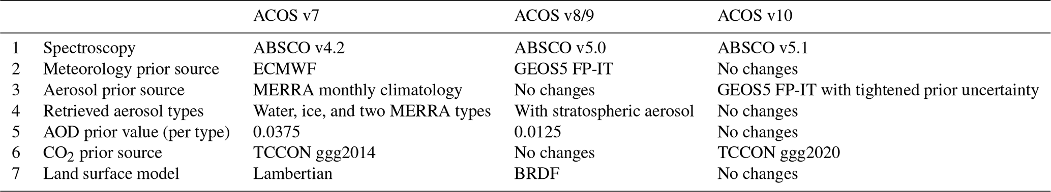
Table 1Evolution of the Atmospheric Carbon Observations from Space (ACOS) Level 2 Full Physics (L2FP) retrieval algorithm (Taylor et al., 2021).
2.1 Datasets
2.1.1 OCO-2 dataset
The Orbiting Carbon Observatory-2 (OCO-2) was launched by the National Aeronautics and Space Administration (NASA) on 2 July 2014 to monitor the concentration of atmospheric CO2 at regional and global levels (Crisp, 2015). It carries a three-channel imaging grating spectrometer that collects high-resolution, bore-sighted spectra of reflected sunlight. Spectra are collected in the molecular oxygen A-band at 0.765 µm and the CO2 bands at 1.61 and 2.06 µm (Hakkarainen et al., 2019). Information from all of these bands is combined to calculate the XCO2. The spatial resolution of OCO-2 is 2.25 km × 1.29 km. More details about the instrument design, calibration approach, in-orbit performance, and measurement principles are provided in a previous study (Crisp, 2015). In this study, we used the OCO-2 Atmospheric Carbon Observations from Space (ACOS)/XCO2 version 10r product that was generated using the ACOS Level 2 Full Physics (L2FP) retrieval algorithm, which used a Bayesian optimal estimation framework to derive estimates of XCO2 from spectral measurements of reflected solar radiation (O'Dell et al., 2012; Crisp et al., 2012). A comprehensive study on the validation of OCO-2 XCO2 retrievals against the Total Carbon Column Observing Network (TCCON) CO2 dataset reported an absolute median difference of less than 0.4 ppm and a root-mean-square (RMS) difference of less than 1.5 ppm between the two datasets (Wunch et al., 2017). Similar experiments have been carried out for the validation of different versions of OCO-2 XCO2 products, and the results have shown that the OCO-2 dataset was consistent and reliable for atmospheric CO2 monitoring (Kiel et al., 2019; O'Dell et al., 2018). The quality and the quantity of the XCO2 product have been improved with the developments in the ACOS FP retrieval algorithm. The latest OCO-2 XCO2 product has single sounding precision of ∼ 0.8 ppm over land and ∼ 0.5 ppm over water, and RMS biases of 0.5–0.7 ppm over both land and water (ODell et al., 2021). The evolution of the ACOS L2FP retrieval algorithm from v7 to v10 is summarized in Table 1.
No major changes were made in the ACOS v9 L2FP retrieval algorithm relative to v8 except for the sampling of the meteorological prior. The trace gas absorption coefficient tables (ABSCO) were updated in various versions of the ACOS L2FP retrieval algorithms. The source of the prior meteorology was changed from the European Center for Medium-Range Weather Forecasts (ECMWF) in ACOS v7 to the NASA Goddard Modeling and Assimilation Office (GMAO) Goddard Earth Observing System (GEOS) Forward Processing – Instrument Team (FP-IT) products for v8 and v9. The aerosol prior source was changed from the GMAO Modern-Era Retrospective analysis for Research and Applications (MERRA) product in v7–9 to Goddard Earth Observing System 5 (GEOS5) FP-IT in v10. Moreover, an additional stratospheric aerosol layer was introduced in ACOS v8–10. The prior value of aerosol optical depth (AOD) for each retrieved aerosol type was lowered from 0.0375 in v7 to 0.0125 in v8–10. The CO2 prior developed by the Total Carbon Column Observing Network (TCCON) team using the ggg2014 algorithm remained same in v7, v8, and v9 of the algorithm. Another major change was switching the land surface model from a purely Lambertian land surface model to a bidirectional reflectance distribution function (BRDF) model (Taylor et al., 2021).
2.1.2 ODIAC dataset
ODIAC is a global emission data product of CO2 emissions from fossil fuel combustion provided with 1 km × 1 km and 1∘ × 1∘ spatial resolutions (Oda, Tomohiro, 2015). It shares country-scale estimates with the Carbon Dioxide Information Analysis Center (CDIAC) but distributes the emissions differently within the countries and includes gridded international bunker emissions (Oda and Maksyutov, 2015). CDIAC distributes the CO2 emissions based on the population density, whereas ODIAC incorporates power plant profiles and nighttime light observations for emission distribution (Wang et al., 2020). ODIAC shows better agreement with the US bottom-up inventory (Gurney et al., 2009) than CDIAC, and it is commonly used in flux inversions (Crowell et al., 2019; Lauvaux et al., 2016; Maksyutov et al., 2013; Takagi et al., 2011). In this study, we used the 2020 version of ODIAC emission dataset that is freely available and can be downloaded from http://db.cger.nies.go.jp/dataset/ODIAC/ (last access: 3 June 2021).
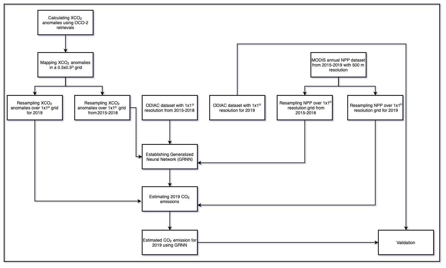
Figure 1Flowchart explaining the steps involved in estimating the anthropogenic CO2 emissions using MODIS NPP and OCO-2 XCO2 retrievals.
2.2 Methods
The estimation of anthropogenic CO2 emissions includes three major steps, as shown in Fig. 1: the first step includes enhancing the XCO2 concentration influenced by anthropogenic activities; the second step involves setting up the GRNN model using the XCO2, NPP, and ODIAC datasets; and the final step is the validation of estimated CO2 emissions against the actual ODIAC emission dataset.
The OCO-2 XCO2 dataset was downloaded from the EARTHDATA platform (https://earthdata.nasa.gov/, last access: 28 May 2021); to ensure the reliability of the data, screening and filtering of the dataset was carried out following the instructions given in the OCO-2 Data User Guide (DUG). Each sounding that is processed using the ACOS L2FP retrieval algorithm is assigned either a “good” (0) or “bad” (1) quality flag based on screening criteria derived from comparisons with TCCON and modeled CO2 fields. It is generally advised that users should use the good-quality soundings for regional- and local-scale studies because the soundings flagged as bad-quality might include biases that compromise their utility for the application. In this study, the OCO-2 XCO2 retrievals were included if (i) they were flagged good (flag of 0) and (ii) the standard deviation of the good soundings for the day was less than 2 ppm. CO2 has a larger background concentration and a longer atmospheric lifetime than other greenhouse gases (Hakkarainen et al., 2019). Hence, XCO2 varies by nearly 2 % over the seasonal cycle and from pole to pole. In addition, XCO2 variations influenced by anthropogenic activities are also smaller on the scale of satellite soundings (2–4 km2). Therefore, high precision is critical for the accurate quantification of the XCO2 anomalies related to anthropogenic activities. To highlight the emission areas, CO2 seasonal variability and the large background concentrations must be removed.
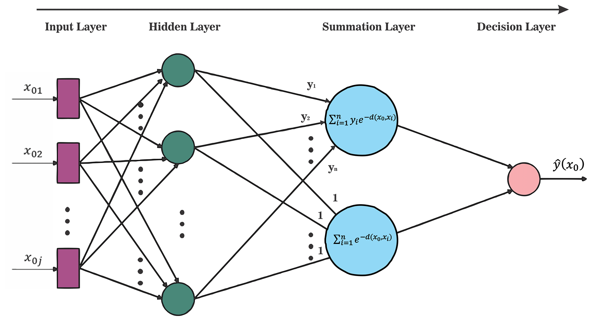
Figure 2Flowchart explaining the steps involved in estimating the anthropogenic CO2 emissions using OCO-2 XCO2 retrievals (Yang et al., 2019).
To highlight the areas associated with the anthropogenic CO2 emission, XCO2 anomalies were calculated by subtracting the daily XCO2 median (daily background) from the individual XCO2 observation – a method suggested by previous studies (Hakkarainen et al., 2019, 2016):
This equation calculated the XCO2 anomalies for each observation. Subtraction of the daily background concentration removes the seasonal variability. The space-based soundings are irregularly distributed and have spatiotemporal gaps because a large amount of the satellite observations is removed after screening for clouds and other artifacts. To deal with the spatiotemporal gaps, kriging interpolation was used, and a mapping dataset was generated with a spatial resolution of 0.5∘ × 0.5∘ (latitude × longitude) and a temporal resolution of 16 d. Finally, the mean of each grid cell was calculated for each year from 2015 to 2019. The annual mean of XCO2 (anomaly) can detrend the seasonal variation (Hakkarainen et al., 2016). The annually averaged XCO2 anomalies were resampled at a grid with a spatial resolution of 1∘ × 1∘ (latitude × longitude) and used along with 1∘ × 1∘ (latitude × longitude) ODIAC emission dataset to set up the GRNN model.
During the process of photosynthesis, living plants convert CO2 into sugar molecules that they use for food. In the process of making food, they also release the oxygen we breathe. Plant productivity plays a crucial role in the global carbon cycle by absorbing the CO2 released by anthropogenic activities. The net primary productivity (NPP) shows how much CO2 is absorbed by plants during photosynthesis minus how much CO2 is released during respiration. A negative NPP value means that CO2 is released into the atmosphere, and a positive value represents the absorption of atmospheric CO2. To improve the model results, an NPP dataset (MOD17A3HGF) provided by MODIS has also been used in this study. It provides information about annual NPP and is distributed by NASA's Land Processes Distributed Active Archive Center (LP DAAC). The NPP dataset with a spatial resolution of 500 m was downloaded from the LP DAAC website (https://lpdaac.usgs.gov/products/mod17a3hgfv006/, last access: 2 September 2021). The annual NPP is derived from the sum of all 8 d Net Photosynthesis (PSN) products (MOD17A2H) from the given year. The MODIS NPP dataset was reprojected and resampled to the spatial resolution of 1∘ × 1∘ (latitude × longitude) for each year and used along with the ODIAC and OCO-2 datasets to train the GRNN model and as well predict the CO2 emissions.
XCO2 variations are primarily influenced by anthropogenic activities and terrestrial ecosystems, and there is both linear and nonlinear mapping between the XCO2 and the emissions. We adopted the GRNN algorithm to represent the nonlinear mapping between the independent variables (XCO2 anomaly and NPP) and the dependent variable (CO2 emissions). The GRNN is a memory-based network that provides estimates of continuous variables and converges to an underlying regression. The regression of a dependent variable on an independent variable is the computation of the most probable value of the dependent variable for each value of the independent variable based on a finite number of possibly noisy measurements of the independent variable and the associated values of the dependent variable. The dependent and the independent variables are usually vectors (Rooki, 2016). The architecture of GRNN is shown in Fig. 2. It consists of four layers including an input layer, a hidden layer, a summation layer, and a decision layer. In the input layer, each neuron corresponds to the independent variable that is expressed as a mathematical function, and the independent variable values are standardized. The standardized values of the independent variable are then transferred to the neurons in the hidden layer. In this layer, each neuron stores the values of the dependent and independent variables and calculates a scalar function. The third layer, known as the summation layer, contains two neurons: the denominator summation unit, which sums the weight values being received from the hidden layer, and the numerator summation unit, which sums the weight values multiplied by the actual target-dependent variable value for each hidden neuron. Finally, the target-dependent value is obtained in the decision layer by dividing the value accumulated in the numerator summation unit by the value in the denominator summation unit. To develop a neural network, the dependent and the independent training variables must be standardized so that all training data will have the same order of magnitude in the input layer (Yang et al., 2019).
where p is the dimension of the variable vector xi, σ is the spread parameter, and an optimal spread parameter value is obtained after several runs following the mean squared error of the estimated values, which must be kept at a minimum (Rooki, 2016). In this study, values of spread parameters were optimized using the “Holdout Method”. More details about the Holdout Method are provided in a previous study (Specht, 1991). The weight of the denominator neuron was set to 1.0. The predicted target dependent variable was defined by the following equation:
where the values calculated with the scalar function in a hidden neuron i are weighted with the corresponding values of the training samples yi. n denotes the number of training samples.
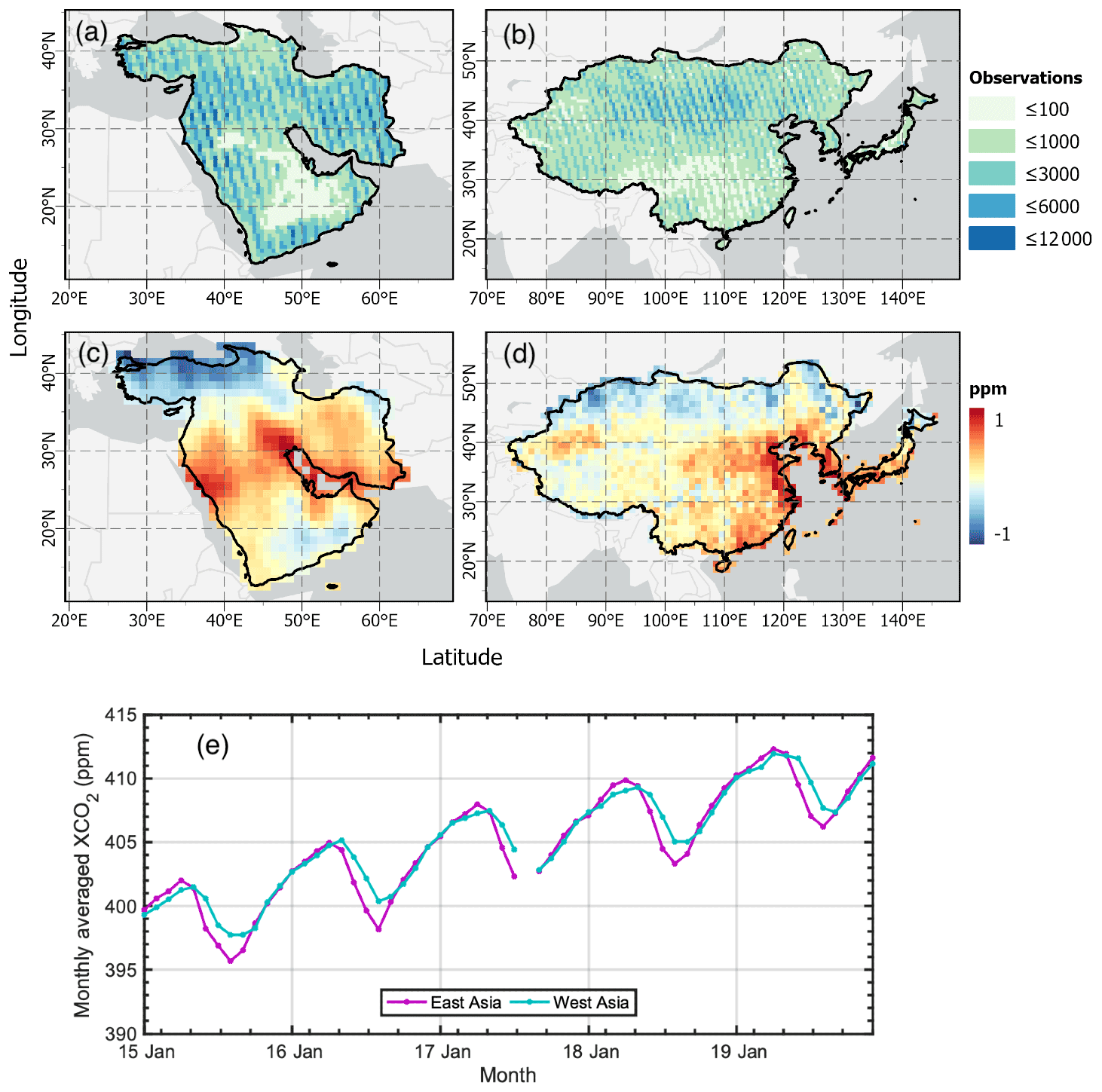
Figure 3Number of observations in each cell of a 0.5 × 0.5∘ grid for a period of 5 years from 2015 to 2019 over (a) West Asia and (b) East Asia; the 5-year mean of XCO2 anomalies calculated using OCO-2 retrievals over (c) West Asia and (d) East Asia; and (e) the monthly averaged XCO2 concentration from 2015 to 2019 over East and West Asia. (The base map was sourced from OpenStreetMap.)
3.1 Spatial distribution of XCO2 observations and anomalies
The satellite-based observations are sensitive to clouds and aerosols; therefore, many of the data are discarded during preprocessing due to the presence of clouds and aerosols (Mustafa et al., 2021b). Figure 3a and b show the quantity of XCO2 retrievals from 2015 to 2019 on a spatial grid of 0.5∘ × 0.5∘ (latitude × longitude) over West and East Asia, respectively. OCO-2 shows good spatial coverage over East Asia; however, the southern parts of the region, in particular the Tibetan Plateau, have a relatively lower number of XCO2 retrievals. The Tibetan Plateau is the most extensively elevated surface on Earth, and satellite measurements show larger uncertainties over this region (Yang et al., 2019). In the case of West Asia, the southern parts of the region have a lower number of XCO2 retrievals. A very large desert, the Rub' al Kahli, is located in this area; it stretches across Saudi Arabia, Yemen, Oman, and the United Arab Emirates (UAE) and often observes dust storms. The lower number of XCO2 retrievals in these parts of the region might be due to the ACOS XCO2 retrieval algorithm that excludes satellite measurements with a high aerosol optical depth and cloud optical thickness (Crisp et al., 2012; O'Dell et al., 2012).
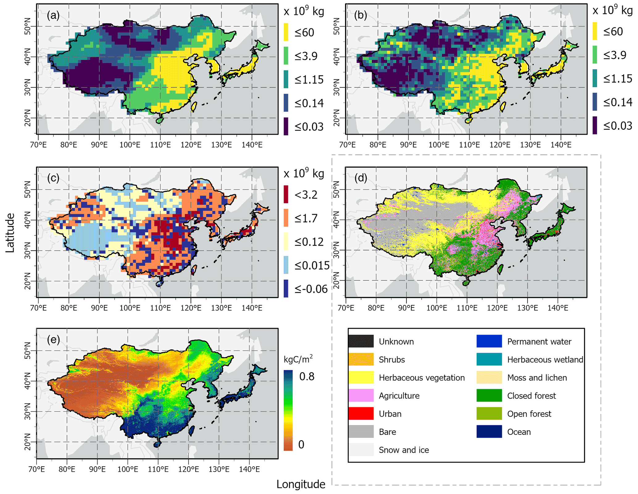
Figure 4Spatial distribution of (a) OCO-2 XCO2-based anthropogenic CO2 emission estimates for 2019, (b) actual ODIAC emissions for 2019, (c) their difference (estimated emission minus actual emission), (d) 100 m resolution land cover distribution provided by the Copernicus Global Land Service over East Asia, and (e) the spatial distribution of NPP. (The base map was sourced from OpenStreetMap.)
Figure 3c shows the spatial distribution of the 5-year averaged XCO2 anomalies calculated using the method described in Sect. 2.2 over West Asia. The higher concentrations of XCO2 anomalies were observed over the central parts of the region that included Iran, Kuwait, Saudi Arabia, and Iraq. Iran and Saudi Arabia are listed among the top 10 CO2 emitting nations and produce over 6 % of the global CO2 emissions (Jalil, 2014). In addition, Iran, Saudi Arabia, and Iraq are the major fuel consumers of the region and contribute more than 60 % of the region's total fossil fuel CO2 emissions (Boden et al., 2017). Figure 4d shows the multiyear averaged XCO2 anomalies over East Asia. The eastern parts of the region including eastern China, Japan, and South Korea show the highest concentrations of XCO2 anomalies. China's Beijing–Tianjin–Hebei area, Korea, and Japan are the most populated urban regions with high amounts of anthropogenic emissions in the world (Mustafa et al., 2020).
Figure 3e shows the monthly averaged XCO2 over East and West Asia. The monthly averaged XCO2 concentrations show seasonal fluctuations. Moreover, the XCO2 concentrations during each month are higher than those in the same month of the previous year, which reflects that the XCO2 concentration in the atmosphere is continuously increasing in both regions. The XCO2 concentration starts increasing from September and reaches its maximum value in April; it then starts decreasing and reaches its minimum value in August. The decrement in its concentration from May to August is due to several reasons; however, it is primarily owing to the strong photosynthesis and weak respiration rate of plants, which is enhanced during the monsoon or rainy season (Mustafa et al., 2020). The increment in the XCO2 concentration from September to April is likely to be caused by weak photosynthesis and strong respiration, the use of heating systems in winter, and strong microbial activity (Cao et al., 2017; Mustafa et al., 2021a).

Figure 5Spatial distribution of (a) OCO-2 XCO2-based anthropogenic CO2 emission estimates for 2019, (b) actual ODIAC emissions for 2019, (c) their difference (estimated emission minus actual emission), (d) 100 m resolution land cover distribution provided by the Copernicus Global Land Service over West Asia, and (e) the spatial distribution of NPP. (The base map was sourced from OpenStreetMap.)
3.2 Estimated CO2 emissions
The annually averaged XCO2 anomalies, MODIS NPP, and ODIAC CO2 emission datasets for a period of 4 years from 2015 to 2018 were used as a training dataset for the GRNN model built to estimate the CO2 emissions using the method described in Sect. 2.2. The GRNN model was then applied to 2019 annually averaged XCO2 anomalies and NPP datasets to predict the CO2 emissions with the same unit as the ODIAC CO2 emissions. The analyses were carried out separately over East and West Asia. Figure 4a and b show the estimated values and the ODIAC CO2 emissions over East Asia, respectively. The results show that the estimated values and the inventory CO2 emissions exhibit nearly the same spatial distribution pattern. The eastern part of the region shows higher CO2 emissions, and the western and northern parts, in particular the Tibetan Plateau and Mongolia, show the minimum CO2 emissions. The pattern is also similar to the XCO2 anomalies distribution over East Asia (Fig. 3d). The estimated CO2 emissions have a relatively smoother distribution pattern compared with the ODIAC CO2 emissions, which might be due to the interpolation of the OCO-2 dataset. Figure 4c shows the difference between the estimated and the inventory CO2 emissions over East Asia. The estimated CO2 emissions are generally overestimated relative to the ODIAC CO2 emissions; however, the emissions are underestimated over some parts of the region as well. Figure 4d shows the land cover distribution of East Asia provided by the Copernicus Global Land Service (Buchhorn et al., 2020). The predicted CO2 emissions are overestimated over most of the regional parts; however, this overestimation is more significant over agricultural areas that are located near high-density regions, e.g., eastern China. Eastern China, Japan, and Korea are known to be among the regions with the highest CO2 emissions, and this underestimation over the agricultural areas might be caused by the nearby CO2 emission sources which raise the CO2 concentration of the nearby areas through atmospheric transport. Previous studies have demonstrated that the concentration of atmospheric CO2 is influenced by atmospheric transport (Cao et al., 2017; Kumar et al., 2014). The areas where the predicted CO2 emissions are underestimated are covered by agriculture, forest, and vegetation. This underestimation of the predicted CO2 emissions over these areas indicates the presence of uncertainties in the XCO2 anomalies that are likely to be produced by the CO2 uptake of the biosphere which still remains in the XCO2 anomalies. In addition, the areas where the estimated CO2 emissions are overestimated have higher elevations. OCO-2 observations show larger uncertainties over elevated and mountainous areas, especially the Tibetan Plateau where the OCO-2 retrievals are significantly overestimated (Kong et al., 2019; Mustafa et al., 2020), and this might also have a contribution to the overestimation of estimated CO2 emissions. The difference between the estimated and the ODIAC CO2 emissions ranged from −0.06 × 10⁹ to 3.2 × 10⁹ kg, and the magnitude of difference between −1 × 10⁹ and 1 × 10⁹ kg accounted for 84 % of the total number of grid cells. Yang et al. (2019) estimated the CO2 emissions using a similar machine learning approach with GOSAT XCO2 retrievals over China, and the differences between the estimated values and the ODIAC CO2 emissions were between −5 × 10⁹ and 5 × 10⁹ kg. Moreover, the predicted results from the abovementioned study exhibited less CO2 emissions overall relative to the ODIAC emissions, contradicting our results. Our study showed better results, which may be due to the fact that (i) we improved the predictive model with the addition of an NPP dataset (Fig. 4e), (ii) we utilized the higher-resolution XCO2 retrievals provided by OCO-2, and (iii) we incorporated the OCO-2 XCO2 retrievals processed using the latest version of the retrieval algorithm. The newer version of the ACOS L2FP retrieval algorithm has improved the quantity and the quality of the satellite-based observations (Taylor et al., 2021).
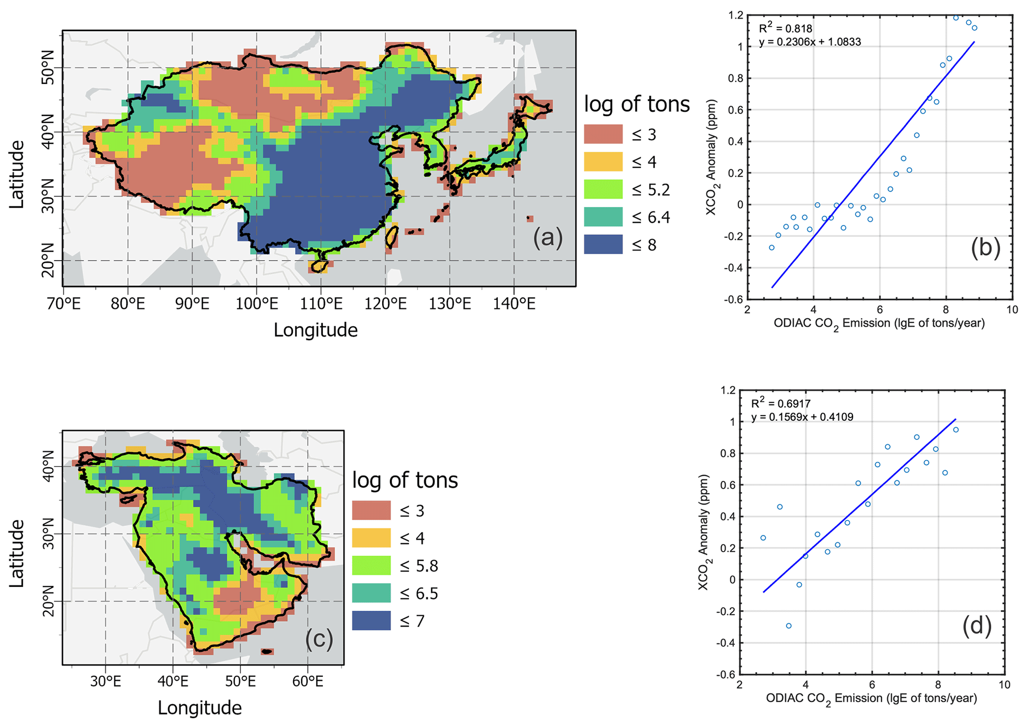
Figure 6The spatial distribution of segmented ODIAC emissions, where the data are binned in 0.3 t yr−1 of lgE (logarithm of base 10) bins using the mean emission calculated from the annual emissions from 2015 to 2019 over (a) East Asia and (c) West Asia. The correlation between mean ODIAC CO2 emissions and mean XCO2 anomalies calculated from annual XCO2 from 2015 to 2018 for (b) East Asia and (d) West Asia. (The base map was sourced from OpenStreetMap.)
Figure 5a and b show the spatial distribution of satellite-based estimated CO2 emissions and the actual ODIAC CO2 emissions over West Asia, respectively. The spatial distribution pattern of both the estimated and the original CO2 emissions is similar with some differences in their magnitudes. CO2 emissions in the eastern parts are relatively larger compared with other parts of the region. Figure 5c shows the difference between the estimated values and the ODIAC CO2 emissions. The satellite-based estimated CO2 emissions are generally overestimated compared with the actual ODIAC CO2 emissions. The estimated CO2 emissions are notably larger over Iran and Saudi Arabia. Figure 5d shows the land cover distribution of West Asia. It can be seen that the predicted CO2 emissions are overestimated over the areas that are covered by either urban settlements or bare land. The overestimation of estimated CO2 over these areas is likely to be caused by atmospheric transportation that influences the spatial distribution of atmospheric CO2 (Cao et al., 2017). Moreover, a large part of West Asia is covered by deserts, and these deserts observe a notably lower number of OCO-2 retrievals (Fig. 3a). The overestimation of the predicted CO2 emissions over the largest desert of the region, the Rub' al Kahli, located in southern parts is likely to be caused by the uncertainties in the satellite-based XCO2 anomalies, and these uncertainties are likely to be produced due to a lower number of OCO-2 retrievals. In addition, a previous study also indicated that the ACOS XCO2 retrieval algorithm showed uncertainties over deserts (Bie et al., 2018). Similar to East Asia, the predicted CO2 emissions over West Asia are also underestimated over areas that are covered by agriculture or vegetation, and this underestimation might be due to the presence of CO2 uptake by the biosphere in the XCO2 anomalies calculated using the satellite-based retrievals. The difference between the estimated values and the ODIAC CO2 emissions ranged from −0.16 × 10⁹ to 2.8 × 10⁹ kg, and the magnitude of the difference between −1 × 10⁹ and 1 × 10⁹ kg accounted for 88 % of the total number of grid cell.
3.3 Correlation analysis between OCO-2 XCO2 anomalies and ODIAC emissions
Figure 6 shows the correlation analysis between the ODIAC CO2 emissions and the XCO2 anomalies calculated using the OCO-2 retrievals over East and West Asia. Yang et al. (2019) found that the cluster of XCO2 changes derived from satellite-based observations showed a better and more significant correlation with the CO2 emissions relative to a single sounding of XCO2, which might have been due to the fact that the atmospheric CO2 measurement is an instantaneous snapshot of the realistic atmosphere (Liu et al., 2015). For the correlation analysis, we segmented the ODIAC emissions, which were binned every 0.3 t yr−1 of lgE (logarithm of base 10) using mean emissions calculated from annual emissions during 2015–2019, and then carried out an analysis between the mean of the emissions and the mean of the XCO2 anomalies within the binned regions. The results showed a positive and significant correlation between the two datasets. Figure 6a and b show the spatial distribution of segmented ODIAC emissions over East Asia and the scatterplot between the mean of the emissions and the mean of the XCO2 anomalies, respectively. The two datasets show a positive and significant correlation with a determined coefficient (R2) of 0.81. The spatial distribution of segmented ODIAC emissions over West Asia and the scatterplot between the mean of the emissions and the mean of the XCO2 anomalies for this region are shown in Fig. 6c and d, respectively. The two datasets showed a good correlation with a determined coefficient (R2) of 0.60. Several studies have correlated satellite-based XCO2 anomalies with CO2 emissions (Fu et al., 2019; Shekhar et al., 2020). Yang et al. (2019) performed a correlation analysis between the GOSAT-based XCO2 anomalies and the ODIAC CO2 emissions over China and found a significant correlation with a determined coefficient (R2) of 0.82 which increased up to 0.95 if the analysis was carried out with higher CO2 emission values. In our study, the correlation between the CO2 emissions and XCO2 anomalies is relatively low for West Asia, which might be due to the uncertainties in the OCO-2 retrievals. A large part of West Asia is covered by deserts, and, as previously stated, Bie et al. (2018) reported that the ACOS XCO2 retrieval algorithm showed uncertainties over deserts.
In this study, anthropogenic CO2 emissions were estimated using satellite datasets and employing a neural-network-based method. The study was carried out using ODIAC CO2 emissions, OCO-2 XCO2, and MODIS NPP datasets from 2015 to 2019. To remove the CO2 seasonal variability and the large background concentration from the OCO-2 XCO2 retrievals, XCO2 anomalies were calculated for each year. A GRNN model was then built; XCO2 anomalies, NPP, and CO2 emissions from 2015 to 2018 were used as a training dataset; and, finally, CO2 emissions were predicted for 2019 based on the NPP and XCO2 anomalies calculated for the same year. The analyses were carried out separately over East and West Asia. The satellite-based estimated values and the ODIAC CO2 emission datasets were compared, and both of the datasets showed good agreement in terms of spatial distribution. The estimated CO2 emissions showed better results over East Asia compared with West Asia, which might be due to the uncertainties in the XCO2 retrievals: previous studies have reported that the ACOS XCO2 retrieval algorithm produced uncertainties over deserts. The predicted CO2 emissions were generally overestimated, and this overestimation was larger over the areas that were closer to the high-density urban regions. The overestimations might be due to the nearby high-emission CO2 sources that raised the XCO2 concentration due to the effects of atmospheric transport. The satellite-based estimated CO2 emissions were underestimated over some parts of the regions, mostly areas covered by agricultural land and vegetation; this was likely caused by the uncertainties in the calculated XCO2 anomalies, and these uncertainties were produced due to the presence of the CO2 uptake of the biosphere. We compared our results with a previous study carried out using a similar predictive model incorporating GOSAT XCO2 retrievals (Yang et al., 2019). The referenced study generally underestimated the predicted CO2 emissions, with larger differences relative to ODIAC CO2 emissions, contradicting our results. Our study showed relatively better results, which might be due to several reasons: (i) we improved the predictive model with the addition of an NPP dataset, (ii) we incorporated OCO-2 XCO2 retrievals that have a higher spatial resolution compared with the GOSAT XCO2 retrievals, and (iii) we used a XCO2 product processed using the latest version of the ACOS L2FP retrieval algorithm. The newer version of the algorithm has improved the quantity and the quality of the XCO2 retrievals. Moreover, correlation analysis was also carried out between the ODIAC CO2 emissions and the OCO-2 XCO2 anomalies, and the results were significant with R2 values of 0.81 and 0.60 over East and West Asia, respectively. These results were in agreement with the previous studies.
The results from our study suggest that CO2 emissions can be estimated using observations obtained from CO2 monitoring satellites. Currently, several satellites are orbiting the Earth and are dedicated to monitoring atmospheric CO2. Joint utilization of the observations from the old and the latest satellites, such as OCO-3, GOSAT-2, and TanSAT, might reduce the spatiotemporal gaps and uncertainties. In future studies, we intend to improve the GRNN model via the addition of CO2 uptake datasets and the joint utilization of multi-sensor data.
The OCO-2 Level 2 XCO2 product is available from https://doi.org/10.5067/E4E140XDMPO2 (OCO-2 Science Team et al., 2020), and the ODIAC CO2 emission dataset is available from http://db.cger.nies.go.jp/dataset/ODIAC/ (CGER, 2021).
FM carried out the analysis under the supervision of LB, with input and support from QW, NY, MS, MB, RWA, and RI. FM wrote the original article with feedback from all the co-authors.
The contact author has declared that neither they nor their co-authors have any competing interests.
Publisher's note: Copernicus Publications remains neutral with regard to jurisdictional claims in published maps and institutional affiliations.
The authors acknowledge the efforts of NASA with respect to providing the OCO-2 data products. The authors are also thankful to the National Institute of Environmental Studies (NIES) for providing the ODIAC CO2 emission dataset. The lead author (Farhan Mustafa) is thankful to Thomas E. Taylor (Colorado State University, USA) for providing help with summarizing the evolution of the ACOS L2FP retrieval algorithm.
This research has been supported by the National Natural Science Foundation of China (NSFC; grant no. 42175145) and the Shanghai Aerospace Science and Technology Innovation Fund (grant no. SAST 2019-045).
This paper was edited by Dmitry Efremenko and reviewed by two anonymous referees.
Bao, Z., Zhang, X., Yue, T., Zhang, L., Wang, Z., Jiao, Y., Bai, W., and Meng, X.: Retrieval and Validation of XCO2 from TanSat Target Mode Observations in Beijing, Remote Sens.-Basel, 12, 3063, https://doi.org/10.3390/rs12183063, 2020.
Bie, N., Lei, L., Zeng, Z., Cai, B., Yang, S., He, Z., Wu, C., and Nassar, R.: Regional uncertainty of GOSAT XCO2 retrievals in China: quantification and attribution, Atmos. Meas. Tech., 11, 1251–1272, https://doi.org/10.5194/amt-11-1251-2018, 2018.
Boden, T. A., Andres, R. J., and Marland, G.: Global, regional, and national fossil-fuel CO2 emissions (1751–2014) (v. 2017), Environmental System Science Data Infrastructure for a Virtual Ecosystem (ESS-DIVE) (United States), Carbon Dioxide Information Analysis Center (CDIAC), Oak Ridge National Laboratory (ORNL), Oak Ridge, TN, USA, 2017.
Bovensmann, H., Buchwitz, M., Burrows, J. P., Reuter, M., Krings, T., Gerilowski, K., Schneising, O., Heymann, J., Tretner, A., and Erzinger, J.: A remote sensing technique for global monitoring of power plant CO2 emissions from space and related applications, Atmos. Meas. Tech., 3, 781–811, https://doi.org/10.5194/amt-3-781-2010, 2010.
Buchhorn, M., Lesiv, M., Tsendbazar, N.-E., Herold, M., Bertels, L., and Smets, B.: Copernicus Global Land Cover Layers—Collection 2, Remote Sens.-Basel, 12, 1044, https://doi.org/10.3390/rs12061044, 2020.
Cao, L., Chen, X., Zhang, C., Kurban, A., Yuan, X., Pan, T., and de Maeyer, P.: The Temporal and Spatial Distributions of the Near-Surface CO2 Concentrations in Central Asia and Analysis of Their Controlling Factors, Atmosphere, 8, 85, https://doi.org/10.3390/atmos8050085, 2017.
Center for Global Environmental Research (CGER): ODIAC Fossil Fuel Emission Dataset, CGER [data set], available at: http://db.cger.nies.go.jp/dataset/ODIAC/, last access: 3 June 2021.
Chen, Z., Ye, X., and Huang, P.: Estimating Carbon Dioxide (CO2) Emissions from Reservoirs Using Artificial Neural Networks, Water, 10, 26, https://doi.org/10.3390/w10010026, 2018.
Crisp, D.: Measuring atmospheric carbon dioxide from space with the Orbiting Carbon Observatory-2 (OCO-2), SPIE Optical Engineering + Applications, San Diego, California, United States, 8 September 2015, 960702, https://doi.org/10.1117/12.2187291, 2015.
Crisp, D., Fisher, B. M., O'Dell, C., Frankenberg, C., Basilio, R., Bösch, H., Brown, L. R., Castano, R., Connor, B., Deutscher, N. M., Eldering, A., Griffith, D., Gunson, M., Kuze, A., Mandrake, L., McDuffie, J., Messerschmidt, J., Miller, C. E., Morino, I., Natraj, V., Notholt, J., O'Brien, D. M., Oyafuso, F., Polonsky, I., Robinson, J., Salawitch, R., Sherlock, V., Smyth, M., Suto, H., Taylor, T. E., Thompson, D. R., Wennberg, P. O., Wunch, D., and Yung, Y. L.: The ACOS CO2 retrieval algorithm – Part II: Global data characterization, Atmos. Meas. Tech., 5, 687–707, https://doi.org/10.5194/amt-5-687-2012, 2012.
Crisp, D., Pollock, H. R., Rosenberg, R., Chapsky, L., Lee, R. A. M., Oyafuso, F. A., Frankenberg, C., O'Dell, C. W., Bruegge, C. J., Doran, G. B., Eldering, A., Fisher, B. M., Fu, D., Gunson, M. R., Mandrake, L., Osterman, G. B., Schwandner, F. M., Sun, K., Taylor, T. E., Wennberg, P. O., and Wunch, D.: The on-orbit performance of the Orbiting Carbon Observatory-2 (OCO-2) instrument and its radiometrically calibrated products, Atmos. Meas. Tech., 10, 59–81, https://doi.org/10.5194/amt-10-59-2017, 2017.
Crowell, S., Baker, D., Schuh, A., Basu, S., Jacobson, A. R., Chevallier, F., Liu, J., Deng, F., Feng, L., McKain, K., Chatterjee, A., Miller, J. B., Stephens, B. B., Eldering, A., Crisp, D., Schimel, D., Nassar, R., O'Dell, C. W., Oda, T., Sweeney, C., Palmer, P. I., and Jones, D. B. A.: The 2015–2016 carbon cycle as seen from OCO-2 and the global in situ network, Atmos. Chem. Phys., 19, 9797–9831, https://doi.org/10.5194/acp-19-9797-2019, 2019.
EDGAR: Emission Database for Global Atmospheric Research (EDGAR v4.3.2), European Commission, 2017.
Fu, P., Xie, Y., Moore, C. E., Myint, S. W., and Bernacchi, C. J.: A Comparative Analysis of Anthropogenic CO2 Emissions at City Level Using OCO-2 Observations: A Global Perspective, Earths Future, 7, 1058–1070, https://doi.org/10.1029/2019EF001282, 2019.
Guan, D., Liu, Z., Geng, Y., Lindner, S., and Hubacek, K.: The gigatonne gap in China's carbon dioxide inventories, Nat. Clim. Change, 2, 672–675, https://doi.org/10.1038/nclimate1560, 2012.
Gurney, K. R., Mendoza, D. L., Zhou, Y., Fischer, M. L., Miller, C. C., Geethakumar, S., and de la Rue du Can, S.: High Resolution Fossil Fuel Combustion CO2 Emission Fluxes for the United States, Environ. Sci. Technol., 43, 5535–5541, https://doi.org/10.1021/es900806c, 2009.
Hakkarainen, J., Ialongo, I., and Tamminen, J.: Direct space-based observations of anthropogenic CO2 emission areas from OCO-2, Geophys. Res. Lett., 43, 11400–11406, https://doi.org/10.1002/2016GL070885, 2016.
Hakkarainen, J., Ialongo, I., Maksyutov, S., and Crisp, D.: Analysis of Four Years of Global XCO2 Anomalies as Seen by Orbiting Carbon Observatory-2, Remote Sens.-Basel, 11, 850, https://doi.org/10.3390/rs11070850, 2019.
Hoegh-Guldberg, O., D. Jacob, M. Taylor, M. Bindi, S. Brown, I. Camilloni, A. Diedhiou, R. Djalante, K.L. Ebi, F. Engelbrecht, J.Guiot, Y. Hijioka, S. Mehrotra, A. Payne, S.I. Seneviratne, A. Thomas, R. Warren, and G. Zhou, 2018: Impacts of 1.5 ∘C Global Warming on Natural and Human Systems, in: Global Warming of 1.5 ∘C. An IPCC Special Report on the impacts of global warming of 1.5 ∘C above pre-industrial levels and related global greenhouse gas emission pathways, in the context of strengthening the global response to the threat of climate change, sustainable development, and efforts to eradicate poverty, edited by: Masson-Delmotte, V., Zhai, P., Pörtner, H.-O., Roberts, D., Skea, J., Shukla, P. R., Pirani, A., Moufouma-Okia, W., Péan, C., Pidcock, R., Connors, S., Matthews, J. B. R., Chen, Y., Zhou, X., Gomis, M. I., Lonnoy, E., Maycock, T., Tignor, M., and Waterfield, T., IPCC, in press, 2021.
Hong, X., Zhang, P., Bi, Y., Liu, C., Sun, Y., Wang, W., Chen, Z., Yin, H., Zhang, C., Tian, Y., and Liu, J.: Retrieval of Global Carbon Dioxide From TanSat Satellite and Comprehensive Validation With TCCON Measurements and Satellite Observations, IEEE T. Geosci. Remote, 1–16, https://doi.org/10.1109/TGRS.2021.3066623, 2021.
Horowitz, C. A.: Paris Agreement, Int. Leg. Mater., 55, 740–755, https://doi.org/10.1017/S0020782900004253, 2016.
Hutchins, M. G., Colby, J. D., Marland, G., and Marland, E.: A comparison of five high-resolution spatially-explicit, fossil-fuel, carbon dioxide emission inventories for the United States, Mitig. Adapt. Strat. Gl., 22, 947–972, https://doi.org/10.1007/s11027-016-9709-9, 2017.
Jalil, S. A.: Carbon Dioxide Emission in the Middle East and North African (MENA) Region: A Dynamic Panel Data Study, Journal of Emerging Economies and Islamic Research, 2, 5, https://doi.org/10.24191/jeeir.v2i3.9629, 2014.
Janssens-Maenhout, G., Crippa, M., Guizzardi, D., Dentener, F., Muntean, M., Pouliot, G., Keating, T., Zhang, Q., Kurokawa, J., Wankmüller, R., Denier van der Gon, H., Kuenen, J. J. P., Klimont, Z., Frost, G., Darras, S., Koffi, B., and Li, M.: HTAP_v2.2: a mosaic of regional and global emission grid maps for 2008 and 2010 to study hemispheric transport of air pollution, Atmos. Chem. Phys., 15, 11411–11432, https://doi.org/10.5194/acp-15-11411-2015, 2015.
Keppel-Aleks, G., Wennberg, P. O., O'Dell, C. W., and Wunch, D.: Towards constraints on fossil fuel emissions from total column carbon dioxide, Atmos. Chem. Phys., 13, 4349–4357, https://doi.org/10.5194/acp-13-4349-2013, 2013.
Kiel, M., O'Dell, C. W., Fisher, B., Eldering, A., Nassar, R., MacDonald, C. G., and Wennberg, P. O.: How bias correction goes wrong: measurement of affected by erroneous surface pressure estimates, Atmos. Meas. Tech., 12, 2241–2259, https://doi.org/10.5194/amt-12-2241-2019, 2019.
Kong, Y., Chen, B., and Measho, S.: Spatio-temporal consistency evaluation of XCO2 retrievals from GOSAT and OCO-2 based on TCCON and model data for joint utilization in carbon cycle research, Atmosphere, 10, 1–23, https://doi.org/10.3390/atmos10070354, 2019.
Konovalov, I. B., Berezin, E. V., Ciais, P., Broquet, G., Zhuravlev, R. V., and Janssens-Maenhout, G.: Estimation of fossil-fuel CO2 emissions using satellite measurements of “proxy” species, Atmos. Chem. Phys., 16, 13509–13540, https://doi.org/10.5194/acp-16-13509-2016, 2016.
Korsbakken, J. I., Peters, G. P., and Andrew, R. M.: Uncertainties around reductions in China's coal use and CO2 emissions, Nat. Clim. Change, 6, 687–690, https://doi.org/10.1038/nclimate2963, 2016.
Kumar, K. R., Revadekar, J. V., and Tiwari, Y. K.: AIRS retrieved CO2 and its association with climatic parameters over india during 2004-2011, Sci. Total Environ., 476–477, 79–89, https://doi.org/10.1016/j.scitotenv.2013.12.118, 2014.
Lamminpää, O., Hobbs, J., Brynjarsdóttir, J., Laine, M., Braverman, A., Lindqvist, H., and Tamminen, J.: Accelerated MCMC for Satellite-Based Measurements of Atmospheric CO2, Remote Sens.-Basel, 11, 2061, https://doi.org/10.3390/rs11172061, 2019.
Lauvaux, T., Miles, N. L., Deng, A., Richardson, S. J., Cambaliza, M. O., Davis, K. J., Gaudet, B., Gurney, K. R., Huang, J., O'Keefe, D., Song, Y., Karion, A., Oda, T., Patarasuk, R., Razlivanov, I., Sarmiento, D., Shepson, P., Sweeney, C., Turnbull, J., and Wu, K.: High-resolution atmospheric inversion of urban CO2 emissions during the dormant season of the Indianapolis Flux Experiment (INFLUX), J. Geophys. Res.-Atmos., 121, 5213–5236, https://doi.org/10.1002/2015JD024473, 2016.
Liu, D., Lei, L., Guo, L., and Zeng, Z.-C.: A Cluster of CO2 Change Characteristics with GOSAT Observations for Viewing the Spatial Pattern of CO2 Emission and Absorption, Atmosphere, 6, 1695–1713, https://doi.org/10.3390/atmos6111695, 2015.
Liu, Y., Wang, J., Yao, L., Chen, X., Cai, Z., Yang, D., Yin, Z., Gu, S., Tian, L., Lu, N., and Lyu, D.: The TanSat mission: preliminary global observations, Sci. Bull., 63, 1200–1207, https://doi.org/10.1016/j.scib.2018.08.004, 2018.
Maksyutov, S., Takagi, H., Valsala, V. K., Saito, M., Oda, T., Saeki, T., Belikov, D. A., Saito, R., Ito, A., Yoshida, Y., Morino, I., Uchino, O., Andres, R. J., and Yokota, T.: Regional CO2 flux estimates for 2009–2010 based on GOSAT and ground-based CO2 observations, Atmos. Chem. Phys., 13, 9351–9373, https://doi.org/10.5194/acp-13-9351-2013, 2013.
Matsunaga, T., Morino, I., Yoshida, Y., Saito, M., Noda, H., Ohyama, H., Niwa, Y., Yashiro, H., Kamei, A., Kawazoe, F., Saeki, T., Ishihara, Y., Imasu, R., Teruyuki, N., Nakajima, T. S. Y., Saitoh, N., and Hashimoto, M.: Early Results of GOSAT-2 Level 2 Products, in: AGU Fall Meeting Abstracts, December 2019, abstract #A52H-02, 2019.
Mustafa, F., Bu, L., Wang, Q., Ali, M. A., Bilal, M., Shahzaman, M., and Qiu, Z.: Multi-year comparison of CO2 concentration from NOAA carbon tracker reanalysis model with data from GOSAT and OCO-2 over Asia, Remote Sens.-Basel, 12, 2498, https://doi.org/10.3390/RS12152498, 2020.
Mustafa, F., Bu, L., Wang, Q., Yao, N., Shahzaman, M., Bilal, M., Aslam, R. W., and Iqbal, R.: Neural Network Based Estimation of Regional Scale Anthropogenic CO2 Emissions Using OCO-2 Dataset Over East and West Asia, Atmos. Meas. Tech. Discuss. [preprint], https://doi.org/10.5194/amt-2021-222, in review, 2021a.
Mustafa, F., Wang, H., Bu, L., Wang, Q., Shahzaman, M., Bilal, M., Zhou, M., Iqbal, R., Aslam, R. W., Ali, M. A., and Qiu, Z.: Validation of GOSAT and OCO-2 against In Situ Aircraft Measurements and Comparison with CarbonTracker and GEOS-Chem over Qinhuangdao, China, Remote Sens.-Basel, 13, 899, https://doi.org/10.3390/rs13050899, 2021b.
OCO-2 Science Team, Gunson, M., and Eldering, A.: OCO-2 Level 2 bias-corrected XCO2 and other select fields from the full-physics retrieval aggregated as daily files, Retrospective processing V10r, Greenbelt, MD, USA, Goddard Earth Sciences Data and Information Services Center (GES DISC) [data set], https://doi.org/10.5067/E4E140XDMPO2, 2020.
ODell, C., Eldering, A., Gunson, M., Crisp, D., Fisher, B., Kiel, M., Kuai, L., Laughner, J., Merrelli, A., Nelson, R., Osterman, G., Payne, V., Rosenberg, R., Taylor, T., Wennberg, P., Kulawik, S., Lindqvist, H., Miller, S., and Nassar, R.: Improvements in XCO2 accuracy from OCO-2 with the latest ACOS v10 product, EGU General Assembly 2021, online, 19–30 Apr 2021, EGU21-10484, https://doi.org/10.5194/egusphere-egu21-10484, 2021.
O'Dell, C. W., Connor, B., Bösch, H., O'Brien, D., Frankenberg, C., Castano, R., Christi, M., Eldering, D., Fisher, B., Gunson, M., McDuffie, J., Miller, C. E., Natraj, V., Oyafuso, F., Polonsky, I., Smyth, M., Taylor, T., Toon, G. C., Wennberg, P. O., and Wunch, D.: The ACOS CO2 retrieval algorithm – Part 1: Description and validation against synthetic observations, Atmos. Meas. Tech., 5, 99–121, https://doi.org/10.5194/amt-5-99-2012, 2012.
O'Dell, C. W., Eldering, A., Wennberg, P. O., Crisp, D., Gunson, M. R., Fisher, B., Frankenberg, C., Kiel, M., Lindqvist, H., Mandrake, L., Merrelli, A., Natraj, V., Nelson, R. R., Osterman, G. B., Payne, V. H., Taylor, T. E., Wunch, D., Drouin, B. J., Oyafuso, F., Chang, A., McDuffie, J., Smyth, M., Baker, D. F., Basu, S., Chevallier, F., Crowell, S. M. R., Feng, L., Palmer, P. I., Dubey, M., García, O. E., Griffith, D. W. T., Hase, F., Iraci, L. T., Kivi, R., Morino, I., Notholt, J., Ohyama, H., Petri, C., Roehl, C. M., Sha, M. K., Strong, K., Sussmann, R., Te, Y., Uchino, O., and Velazco, V. A.: Improved retrievals of carbon dioxide from Orbiting Carbon Observatory-2 with the version 8 ACOS algorithm, Atmos. Meas. Tech., 11, 6539–6576, https://doi.org/10.5194/amt-11-6539-2018, 2018.
Oda, T.: ODIAC Fossil Fuel CO2 Emissions Dataset (ODIAC2020, ODIAC2019, ODIAC2018, ODIAC2017, ODIAC2016, ODIAC2015a, ODIAC2013a), National Institute for Environmental Studies, Japan [data set], https://doi.org/10.17595/20170411.001, 2015.
Oda, T., Maksyutov, S., and Andres, R. J.: The Open-source Data Inventory for Anthropogenic CO2, version 2016 (ODIAC2016): a global monthly fossil fuel CO2 gridded emissions data product for tracer transport simulations and surface flux inversions, Earth Syst. Sci. Data, 10, 87–107, https://doi.org/10.5194/essd-10-87-2018, 2018.
Olivier, J. G. J., Van Aardenne, J. A., Dentener, F. J., Pagliari, V., Ganzeveld, L. N., and Peters, J. A. H. W.: Recent trends in global greenhouse gas emissions:regional trends 1970–2000 and spatial distributionof key sources in 2000, Environm. Sci., 2, 81–99, https://doi.org/10.1080/15693430500400345, 2005.
Peylin, P., Law, R. M., Gurney, K. R., Chevallier, F., Jacobson, A. R., Maki, T., Niwa, Y., Patra, P. K., Peters, W., Rayner, P. J., Rödenbeck, C., van der Laan-Luijkx, I. T., and Zhang, X.: Global atmospheric carbon budget: results from an ensemble of atmospheric CO2 inversions, Biogeosciences, 10, 6699–6720, https://doi.org/10.5194/bg-10-6699-2013, 2013.
Rao, M.: Machine Learning in Estimating CO2 Emissions from Electricity Generation, in: Uncertainty Management in Engineering – Topics in Pollution Prevention and Controls [Working Title], IntechOpen, https://doi.org/10.5772/intechopen.97452, 2021.
Rooki, R.: Application of general regression neural network (GRNN) for indirect measuring pressure loss of Herschel–Bulkley drilling fluids in oil drilling, Measurement, 85, 184–191, https://doi.org/10.1016/j.measurement.2016.02.037, 2016.
Shan, Y., Guan, D., Zheng, H., Ou, J., Li, Y., Meng, J., Mi, Z., Liu, Z., and Zhang, Q.: China CO2 emission accounts 1997–2015, Sci. Data, 5, 170201, https://doi.org/10.1038/sdata.2017.201, 2018.
Shekhar, A., Chen, J., Paetzold, J. C., Dietrich, F., Zhao, X., Bhattacharjee, S., Ruisinger, V., and Wofsy, S. C.: Anthropogenic CO2 emissions assessment of Nile Delta using XCO2 and SIF data from OCO-2 satellite, Environ. Res. Lett., 15, 095010, https://doi.org/10.1088/1748-9326/ab9cfe, 2020.
Specht, D. F.: A general regression neural network, IEEE T. Neural Networ., 2, 568–576, https://doi.org/10.1109/72.97934, 1991.
Takagi, H., Saeki, T., Oda, T., Saito, M., Valsala, V., Belikov, D., Saito, R., Yoshida, Y., Morino, I., Uchino, O., Andres, R. J., Yokota, T., and Maksyutov, S.: On the Benefit of GOSAT Observations to the Estimation of Regional CO2 Fluxes, SOLA, 7, 161–164, https://doi.org/10.2151/sola.2011-041, 2011.
Taylor, T. E., Eldering, A., Merrelli, A., Kiel, M., Somkuti, P., Cheng, C., Rosenberg, R., Fisher, B., Crisp, D., Basilio, R., Bennett, M., Cervantes, D., Chang, A., Dang, L., Frankenberg, C., Haemmerle, V. R., Keller, G. R., Kurosu, T., Laughner, J. L., Lee, R., Marchetti, Y., Nelson, R. R., O'Dell, C. W., Osterman, G., Pavlick, R., Roehl, C., Schneider, R., Spiers, G., To, C., Wells, C., Wennberg, P. O., Yelamanchili, A., and Yu, S.: OCO-3 early mission operations and initial (vEarly) XCO2 and SIF retrievals, Remote Sen. Environ., 251, 112032, https://doi.org/10.1016/j.rse.2020.112032, 2020.
Taylor, T. E., O'Dell, C. W., Crisp, D., Kuze, A., Lindqvist, H., Wennberg, P. O., Chatterjee, A., Gunson, M., Eldering, A., Fisher, B., Kiel, M., Nelson, R. R., Merrelli, A., Osterman, G., Chevallier, F., Palmer, P. I., Feng, L., Deutscher, N. M., Dubey, M. K., Feist, D. G., Garcia, O. E., Griffith, D., Hase, F., Iraci, L. T., Kivi, R., Liu, C., De Mazière, M., Morino, I., Notholt, J., Oh, Y.-S., Ohyama, H., Pollard, D. F., Rettinger, M., Roehl, C. M., Schneider, M., Sha, M. K., Shiomi, K., Strong, K., Sussmann, R., Té, Y., Velazco, V. A., Vrekoussis, M., Warneke, T., and Wunch, D.: An eleven year record of XCO2 estimates derived from GOSAT measurements using the NASA ACOS version 9 retrieval algorithm, Earth Syst. Sci. Data Discuss. [preprint], https://doi.org/10.5194/essd-2021-247, in review, 2021.
Wang, J. S., Oda, T., Kawa, S. R., Strode, S. A., Baker, D. F., Ott, L. E., and Pawson, S.: The impacts of fossil fuel emission uncertainties and accounting for 3-D chemical CO2 production on inverse natural carbon flux estimates from satellite and in situ data, Environ. Res. Lett., 15, 085002, https://doi.org/10.1088/1748-9326/ab9795, 2020.
Wang, R., Tao, S., Ciais, P., Shen, H. Z., Huang, Y., Chen, H., Shen, G. F., Wang, B., Li, W., Zhang, Y. Y., Lu, Y., Zhu, D., Chen, Y. C., Liu, X. P., Wang, W. T., Wang, X. L., Liu, W. X., Li, B. G., and Piao, S. L.: High-resolution mapping of combustion processes and implications for CO2 emissions, Atmos. Chem. Phys., 13, 5189–5203, https://doi.org/10.5194/acp-13-5189-2013, 2013.
Wunch, D., Wennberg, P. O., Osterman, G., Fisher, B., Naylor, B., Roehl, C. M., O'Dell, C., Mandrake, L., Viatte, C., Kiel, M., Griffith, D. W. T., Deutscher, N. M., Velazco, V. A., Notholt, J., Warneke, T., Petri, C., De Maziere, M., Sha, M. K., Sussmann, R., Rettinger, M., Pollard, D., Robinson, J., Morino, I., Uchino, O., Hase, F., Blumenstock, T., Feist, D. G., Arnold, S. G., Strong, K., Mendonca, J., Kivi, R., Heikkinen, P., Iraci, L., Podolske, J., Hillyard, P. W., Kawakami, S., Dubey, M. K., Parker, H. A., Sepulveda, E., García, O. E., Te, Y., Jeseck, P., Gunson, M. R., Crisp, D., and Eldering, A.: Comparisons of the Orbiting Carbon Observatory-2 (OCO-2) measurements with TCCON, Atmos. Meas. Tech., 10, 2209–2238, https://doi.org/10.5194/amt-10-2209-2017, 2017.
Yang, D., Liu, Y., Cai, Z., Chen, X., Yao, L., and Lu, D.: First Global Carbon Dioxide Maps Produced from TanSat Measurements, Adv. Atmos. Sci., 35, 621–623, https://doi.org/10.1007/s00376-018-7312-6, 2018.
Yang, S., Lei, L., Zeng, Z., He, Z., and Zhong, H.: An Assessment of Anthropogenic CO2 Emissions by Satellite-Based Observations in China, Sensors-Basel, 19, 1118, https://doi.org/10.3390/s19051118, 2019.