the Creative Commons Attribution 4.0 License.
the Creative Commons Attribution 4.0 License.
 | 21 Dec 2021
Phosgene distribution derived from MIPAS ESA v8 data: intercomparisons and trends
Paolo Pettinari
Flavio Barbara
Simone Ceccherini
Bianca Maria Dinelli
Marco Gai
Piera Raspollini
Luca Sgheri
Massimo Valeri
Gerald Wetzel
Nicola Zoppetti
Marco Ridolfi
The Michelson Interferometer for Passive Atmospheric Sounding (MIPAS) measured the middle-infrared limb emission spectrum of the atmosphere from 2002 to 2012 on board ENVISAT, a polar-orbiting satellite. Recently, the European Space Agency (ESA) completed the final reprocessing of MIPAS measurements, using version 8 of the level 1 and level 2 processors, which include more accurate models, processing strategies, and auxiliary data. The list of retrieved gases has been extended, and it now includes a number of new species with weak emission features in the MIPAS spectral range. The new retrieved trace species include carbonyl chloride (COCl2), also called phosgene. Due to its toxicity, its use has been reduced over the years; however, it is still used by chemical industries for several applications. Besides its direct injection in the troposphere, stratospheric phosgene is mainly produced from the photolysis of CCl4, a molecule present in the atmosphere because of human activity. Since phosgene has a long stratospheric lifetime, it must be carefully monitored as it is involved in the ozone destruction cycles, especially over the winter polar regions.
In this paper we exploit the ESA MIPAS version 8 data in order to discuss the phosgene distribution, variability, and trends in the middle and lower stratosphere and in the upper troposphere. The zonal averages show that phosgene volume mixing ratio is larger in the stratosphere, with a peak of 40 pptv (parts per trillion by volume) between 50 and 30 hPa at equatorial latitudes, while at middle and polar latitudes it varies from 10 to 25 pptv. A moderate seasonal variability is observed in polar regions, mostly between 80 and 50 hPa. The comparison of MIPAS–ENVISAT COCl2 v8 profiles with the ones retrieved from MIPAS balloon and ACE-FTS (Atmospheric Chemistry Experiment – Fourier Transform Spectrometer) measurements highlights a negative bias of about 2 pptv, mainly in polar and mid-latitude regions. Part of this bias is attributed to the fact that the ESA level 2 v8 processor uses an updated spectroscopic database. For the trend computation, a fixed pressure grid is used to interpolate the phosgene profiles, and, for each pressure level, VMR (volume mixing ratio) monthly averages are computed in pre-defined 10∘ wide latitude bins. Then, for each latitudinal bin and pressure level, a regression model has been fitted to the resulting time series in order to derive the atmospheric trends. We find that the phosgene trends are different in the two hemispheres. The analysis shows that the stratosphere of the Northern Hemisphere is characterized by a negative trend of about −7 pptv per decade, while in the Southern Hemisphere phosgene mixing ratios increase with a rate of the order of +4 pptv per decade. This behavior resembles the stratospheric trend of CCl4, which is the main stratospheric source of COCl2. In the upper troposphere a positive trend is found in both hemispheres.
- Article
(3523 KB) - Full-text XML
- BibTeX
- EndNote


Phosgene (COCl2) is a poisonous gas that was used as chemical weapon during the First World War (Fitzgerald, 2008). Today, it is still used by chemical industries, in particular in insecticides, in herbicides, and for pharmaceuticals preparation, even though its use has declined over the years.
The major source of atmospheric phosgene production is the decomposition of chlorocarbon compounds. In particular, the photolysis of carbon tetrachloride (CCl4) and the reaction between methyl chloroform (CH3CCl3) and hydroxyl radical (OH) are its main sources in the lower stratosphere, where phosgene peaks. Losses of phosgene in the stratosphere occur via photodissociation to produce ClO (Fu et al., 2007). However, since phosgene does not react with OH and since it is a weak absorber of ultraviolet radiation, the vertical transport is faster than this process (Kindler et al., 1995). The main loss mechanisms of COCl2 in the troposphere are the hydrolysis in cloud water and ocean deposition (Toon et al., 2001).
Phosgene is also produced, to a lesser extent, from the atmospheric degradation of the anthropogenic chlorinated very short-lived substances (VSLSs), which have a tropospheric lifetime under 6 months. Namely, these are dichloromethane (methylene chloride, CH2Cl2), chloroform (trichloromethane, CHCl3), tetrachloroethene (perchloroethylene, CCl2CCl2, shortened to C2Cl4), trichloroethene (C2HCl3), and dichloroethane (CH2ClCH2Cl), the most abundant of them being CH2Cl2, (65 % of the whole chlorinated VSLS budget), then CHCl3 (20 %), and CH2ClCH2Cl (13 %). Degradation of these substances to produce COCl2 and HCl may occur either in the troposphere, where the resulting products are then injected in the stratosphere (product gas injection, PGI), or in the stratosphere (source gas injection, SGI). Although industrial emissions of all chlorinate VSLSs except CHCl3 dominate over natural sources, these compounds are not yet regulated; therefore, the concentration of some of them is increasing in the atmosphere (Engel and Rigby, 2019). Even if the contribution of chlorinated VSLSs to the total tropospheric chlorine (Cl) is approximately only 3 % (Engel and Rigby, 2019), their relative contribution to the Cl abundance may increase in the future, when the concentration of substances regulated by the Montreal Protocol will be significantly reduced.
Singh (1976) performed the first in situ measurement of atmospheric phosgene concentrations. Phosgene data acquired 12 years later from aircraft revealed a discrepancy between its measurement and the concentrations predicted on the basis of the CCl4 photochemical breakdown alone (Wilson et al., 1988). A total of 12 phosgene profiles were recorded by the MklV spectrometer during nine balloon flights between 1992 and 2000, at latitudes near 34 and 68∘ N, using the solar occultation technique (Toon et al., 2001). Recently, a long-term record (2004–2016) of COCl2 observations was obtained from the measurements of the Atmospheric Chemistry Experiment – Fourier Transform Spectrometer (ACE-FTS) (Harrison et al., 2019).
Long-term records are important to study the COCl2 temporal variation that, in turn, provides information on the temporal variation in the substances responsible for its production, namely CCl4, CH3CCl3, and Cl-containing VSLSs. Recently Harrison et al. (2019) estimated the trend of COCl2 from ACE-FTS measurements in the period 2004–2016 and compared the results with the TOMCAT/SLIMCAT three-dimensional chemical transport model (CTM). A negative COCl2 trend was found in the stratosphere and a positive trend in the upper troposphere, compatible with TOMCAT results when VSLSs are taken into account. The authors also identified a positive bias of 10–20 pptv (parts per trillion by volume) of the ACE-FTS measurements with respect to the model data.
Due to the solar occultation technique used by ACE-FTS, its measurements are denser over the polar regions, with relatively poor coverage in the tropics. For the estimation of global data and trends, the ACE-FTS sparse spatial sampling makes the averaging of the occultation data for periods of several months necessary, both to reduce the random error down to acceptable levels and to enhance the density of its coverage. The Michelson Interferometer for Passive Atmospheric Sounding (MIPAS) covers the spectral region where phosgene signatures are present; therefore, its measurements can also be used to retrieve the phosgene vertical distribution (Valeri et al., 2016). MIPAS measured the middle-infrared limb emission spectrum of the atmosphere on board the European Space Agency (ESA) Environmental Satellite (ENVISAT) from 2002 to 2012. Being based on the observation of the infrared limb emission, MIPAS–ENVISAT data are quite dense and uniform both in space and time, providing a better temporal and spatial coverage than the ACE-FTS measurements. Due to the lower intensity of the measured signal, the individual MIPAS spectra show a lower signal to noise ratio (SNR) than the ACE-FTS ones. Despite the larger noise error of the MIPAS profiles retrieved from single scans, Valeri et al. (2016) showed that high-vertical-resolution, good-quality distributions of COCl2 can be obtained by MIPAS on a per profile basis. Therefore, Valeri et al. (2016) were able to study the seasonality and the latitudinal distribution of phosgene based on a restricted set of MIPAS measurements: the data acquired over 2 d month−1 in the year 2008.
Recently, ESA completed the final full MIPAS mission re-analysis with version 8 of both the level 1 and level 2 processors. As compared to earlier versions, these processors include several new features, leading to a significant improvement in the products' accuracy (Raspollini et al., 2021). Among the new features, the list of retrieved atmospheric constituents has been significantly extended, and, based on the work of Valeri et al. (2016), also phosgene has been included. In this work we analyze the MIPAS level 2 v8 phosgene dataset (Dinelli, 2021) in terms of global distribution, seasonality, and trends.
Here, the paper organization is described. In Sect. 2 MIPAS measurements are introduced. In Sect. 3 the phosgene mean global distribution and seasonality at different latitudes are discussed. In Sect. 4 MIPAS phosgene profiles are compared to those retrieved from ACE-FTS and MIPAS balloon (MIPAS-B) measurements. In Sect. 5 the trend estimation strategy is illustrated, and the results are discussed. Finally, in Sect. 6 the analysis conclusions are drawn.
The Fourier transform spectrometer MIPAS (Fischer et al., 2008), on board the European satellite ENVISAT which flew in a polar sun-synchronous orbit, acquired atmospheric limb emission spectra from July 2002 to April 2012 in the mid-infrared region, from 680 to 2410 cm−1. In the first period of the MIPAS mission, between July 2002 and March 2004, measurements were acquired, almost continuously, at the full spectral resolution (FR) of 0.025 cm−1. This measurement strategy was stopped on 26 March 2004 due to a mechanical problem in the interferometer drive unit. In January 2005, measurements were resumed with a reduced spectral resolution of 0.0625 cm−1. Since the new measurement strategy was faster than the FR one, the spatial sampling was increased, and the new measurements, acquired after January 2005, belong to the so called optimized resolution (OR) period. In addition to the finer horizontal and vertical spatial sampling, the OR measurements have also a reduced noise-equivalent spectral radiance (NESR). Details regarding FR and OR MIPAS measurements can be found in Raspollini et al. (2013), Raspollini et al. (2021), and Dinelli (2021). The important aspect is that MIPAS data, acquired during both mission phases, have a dense coverage over the whole globe, allowing us to study the atmospheric composition and its evolution in great detail. In particular, about 950 profiles per day are measured during the FR period and about 1350 profiles per day during the OR period.
Radiometrically calibrated and geolocated spectra are created by the level 1b processor (Kleinert et al., 2007) from the MIPAS interferograms. Version 8 of the level 1b processor includes several improvements as compared to earlier versions (Kleinert et al., 2018). The most relevant for our analysis is the detector nonlinearity correction. Since photoconductive detectors are subject to aging, their response slowly decreases with time and becomes more linear as a function of the input signal. If not properly corrected, this effect causes a drift of the instrument response and thus of the retrieved profile values. Starting from version 7 of the level 1b processor, time-dependent coefficients, determined from in-flight characterization, are used to correct for detector nonlinearity. In the level 1b processor version 8, the algorithm used to compute these coefficients has been further refined. Now it accounts for the actual instrument temperature and for the degree of ice contamination. This correction leads to a further reduction in the drift caused by the progressive aging of the photoconductive detectors. Now the drift error is estimated to be less than 0.5 % across the entire MIPAS mission (Kleinert et al., 2018).
The calibrated level 1b limb emission spectral radiances are further processed by the ESA level 2 processor version 8 that now coincides with the scientific prototype code named the optimized retrieval model (ORM; Ridolfi et al., 2000; Raspollini et al., 2006, 2013). Full details and an assessment of the improvements implemented in the ORM version 8 (v8) as compared to earlier versions are provided in Raspollini et al. (2021). Here we only list the main new features of the ORM v8, which are relevant to the results presented in this paper:
-
use of the optimal estimation method (Rodgers, 2000) to retrieve the volume mixing ratio (VMR) of gases with extremely low signal to noise ratio;
-
modeling of the horizontal variability in the atmosphere using horizontal gradients of temperature, ozone, and water vapor, extracted from ECMWF ERA Interim reanalysis at the geolocation and time of each limb scan measurement;
-
use of latitude- and height-dependent cloud-index thresholds to detect and filter limb measurements affected by clouds;
-
use of the updated spectroscopic database HITRAN_mipas_pf4.45 (Raspollini et al., 2021), containing in particular updated data for COCl2 (Tchana et al., 2015) and HNO3 (Perrin et al., 2016), now contained also in HITRAN_2016 database (Gordon et al., 2017); updated absorption cross-section data for some heavy molecules: CFC−11 (Harrison, 2018) and CFC−113 (Bris et al., 2011), as well as CFC−12, CFC−14, CCl4, HCFC−22, ClONO2, and HNO4 taken from HITRAN 2016 (Gordon et al., 2017).
As reported in Dinelli (2021), for the retrieval of COCl2, the optimal estimation functionality of the ORM v8 has been exploited. The a priori COCl2 profile used is a global climatological average (Remedios et al., 2007; Raspollini et al., 2021), independent of both latitude and time. The choice of using a fixed a priori profile to process all measurements guarantees that the observed variability in the retrieved profiles can be solely ascribed to the variability in the measurements. The covariance matrix representing the a priori error has been built assuming an error made of two components: an absolute, altitude-independent component of 1 pptv and a relative component equal to the 95 % of the a priori profile. The off-diagonal elements of this covariance matrix are computed assuming a vertical correlation length of 6 km.
The COCl2 retrieval is performed using optimized spectral intervals (microwindows, MWs) chosen by the MWMAKE algorithm (Dudhia et al., 2002), which selects MWs by minimizing a cost function that takes into account the total retrieval error achieved when a given test set of MWs is used at specific tangent heights. Therefore, the algorithm also provides an optimized vertical range for the retrieval and the resulting error components of the retrieved profile. The MWs selected for COCl2 retrieval are listed in Table 1. Note that, due to recent updates in the MWMAKE algorithm and in its assumed error figures (Dudhia, 2019), the selected MWs are different from those used in the work of Valeri et al. (2016). The selection process of the new MWs has removed the strong interference of the CFC−11 emissions found by Valeri et al. (2016), enabling the retrieval of COCl2 as a single target. The vertical retrieval range for COCl2 is from 6 to 36 km for the FR measurements and from 9 to 54 km for the OR measurements.
Table 1Microwindows used for the COCl2 retrievals of FR (left column) and OR (right column) measurements.
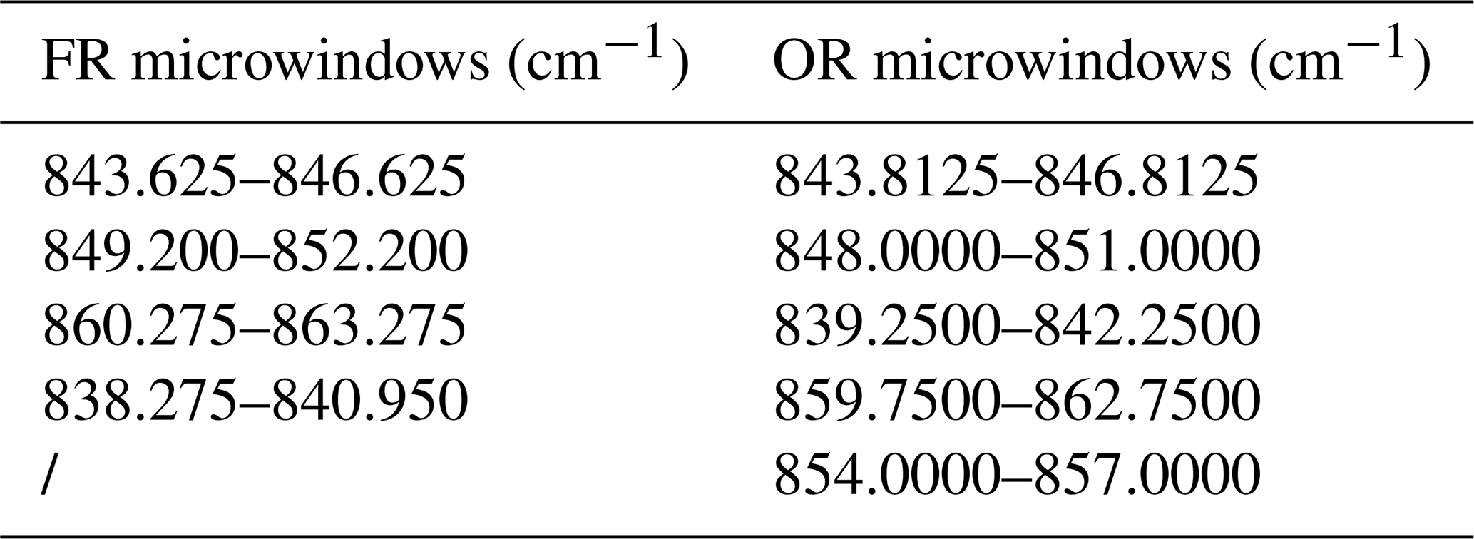
Figure 1 shows the most relevant error components affecting the phosgene mid-latitude day profiles for the FR (Fig. 1a) and OR (Fig. 1b) MIPAS measurements. In Fig. 1, the error propagating from the measurement noise is labeled as “noise”, and the errors induced by uncertainties in the assumed temperature and pressure profiles are labeled “pt”. The errors due to the uncertainty in the spectrally interfering gases are labeled with the gas name on the plot's labels. The label “hialtx” refers to the error due to assuming the climatological profile shape above the highest point of the retrieval grid, “nonlte” is the error arising from the local thermal equilibrium assumption in the radiative transfer model, “lut” is the error due to using the radiative transfer cross-section lookup tables (LUTs) compressed with the truncated singular value decomposition method, “gain-a” is the error in the radiometric calibration of the instrument, and, finally, “spcdb” is the error due to the uncertainties in the spectroscopic parameters. A more exhaustive list and a more thorough description of the various error components are presented in Dudhia (2019). All the errors presented in Fig. 1, except the “noise” and the “pt” errors, have been calculated by MWMAKE by propagating the uncertainties coming from both the instrument and the radiative transfer model onto the retrieved profiles. The “noise” and “pt” errors are a yearly average of the “noise” and “pt” error components, as computed by the ORM v8 (Raspollini et al., 2021). In Fig. 1, we can see a pronounced peak of the “pt” error component mainly observed in the OR period. It is caused by an increased sensitivity to “pt” variations in the VMR between 25 and 30 km, and it is larger in the OR period due to both the different MWs (see Table 1) and the finer limb scan pattern implemented in the OR part of the mission.
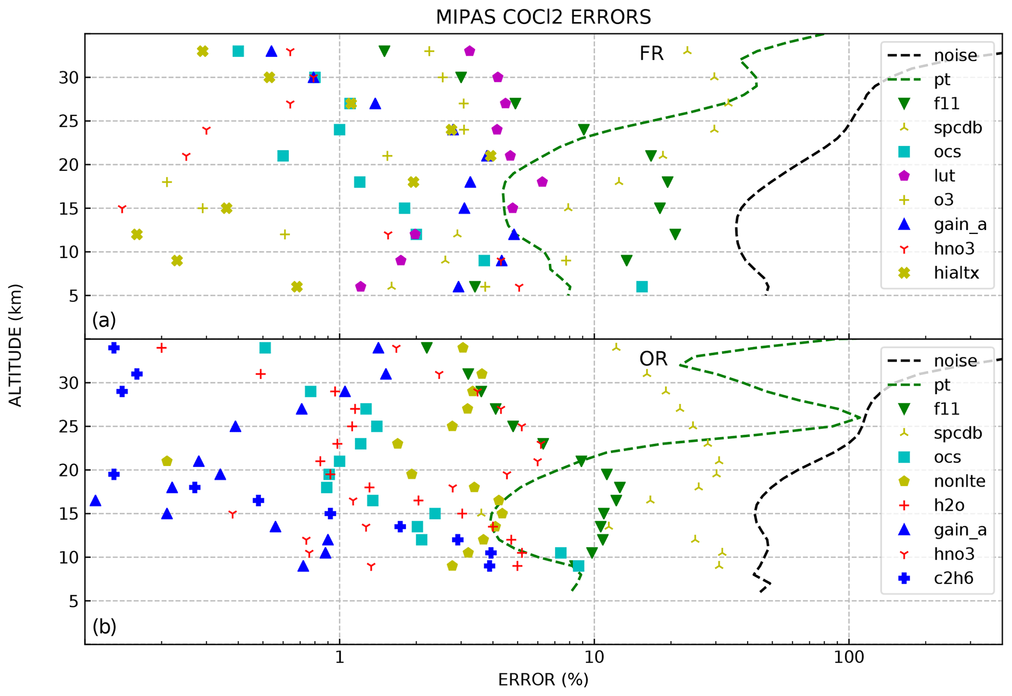
Figure 1Error components affecting the individual retrieved COCl2 profiles in mid-latitude day conditions. Panel (a) refers to FR and panel (b) to OR measurements.
The most important contributions to the total error are due to the measurement noise, to the error in tangent pressures and the temperature profile (“pt”), and to the spectroscopic errors (“spcdb”). Although most of the error components remain quite constant with the season and latitude, some differences exist. Information about the error analysis in different scenarios can be found in Dudhia (2019). When the retrieved profiles are averaged, the individual error components combine differently according to their variability from profile to profile. In our analysis, “noise”, “pt”, and all errors due to the interference with other gases, for example “ocs” or “f11”, are considered as random; i.e., in the averages they are assumed to decrease inversely to the square root of the number of averaged profiles. Indeed, interference uncertainties depend on the difference between the assumed and real concentrations of the interfering gas, which is expected to change from scan to scan. On the other hand, spectroscopic (“spcdb”), lookup table (“lut”), and radiometric calibration (“gain-a”) errors do not change from profile to profile; thus they are assumed to be systematic and are not damped in the averaging process.
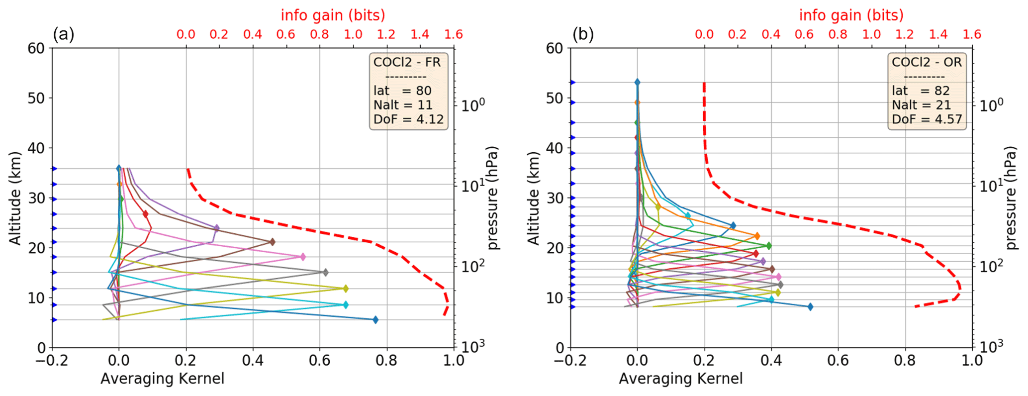
Figure 2Typical AKs of individual COCl2 profiles retrieved from FR (a) and OR (b) MIPAS measurements. The dashed red lines represent the information gain due to the retrieval.
The averaging kernel (AK) matrix represents a linear approximation of the vertical response function that characterizes the measurement chain (Rodgers, 2000; Ceccherini and Ridolfi, 2010). Both the instrument and the retrieval characteristics contribute to the AK. With the retrieval setup described above, the individual phosgene profiles retrieved show typical AKs (rows of the AK matrix) as in Fig. 2 for the FR (Fig. 2a) and OR (Fig. 2b) mission phases. AK peak values approaching unity denote heights where the contribution of the measurements to the retrieval is significantly larger than that of the a priori information. The trace of the AK matrix quantifies the number of degrees of freedom (DOFs) of the retrieval, i.e., the number of independent pieces of information on the profile extracted from the measurements. As indicated in the plot's key, the number of DOFs of the individual profiles is around 4. The vertical resolution of the retrieved profiles can be estimated on the basis of the full width at half maximum (FWHM) of the AKs using the formula proposed in Eq. (8) of Ridolfi and Sgheri (2009). According to that equation, wider AKs correspond to lower vertical resolution. In particular, the vertical resolution of the FR (OR) period is about 5 km (3.5 km) below 17 km. It starts to degrade with the altitude, reaching 10 km at the altitude of 25 km. Indeed, Fig. 2 shows that the AK diagonal elements become smaller and smaller as altitude increases. For this reason, although the retrieval is performed up to 36 (FR) and 54 km (OR), in our analysis we only use COCl2 profiles retrieved inside its useful range (Dinelli, 2021), which is below 28 km. The dashed red lines represent the information gain, defined in Dinelli et al. (2010). It provides an estimate of the information gain due to the measurement with respect to the a priori knowledge. Its value is zero when the retrieval and a priori errors are equal, and it increases when the retrieval error reduces. We can see that the information gain decreases with the altitude, denoting the important role of the a priori profile at high altitudes.
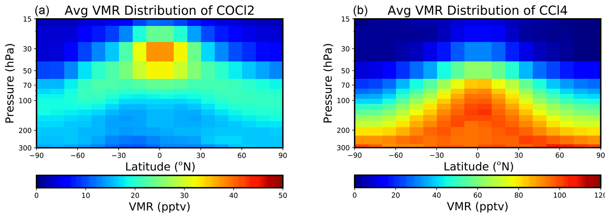
Figure 3COCl2 (a) and CCl4 (b) global distributions. Average over the whole MIPAS mission period (2002–2012).
We interpolated each of the retrieved COCl2 profiles to the SPARC data initiative (Hegglin et al., 2013) pressure grid, consisting of the following 28 levels: 300, 250, 200, 170, 150, 130, 115, 100, 90, 80, 70, 50, 30, 20, 15, 10, 7, 5, 3, 2, 1.5, 1, 0.7, 0.5, 0.3, 0.2, 0.15, and 0.1 hPa. Then, we grouped the interpolated profiles into 18 latitude bins, each 10∘ wide. For each pressure level and latitude bin, we computed the COCl2 average VMR over the whole MIPAS mission. Figure 3a shows the global vertical distribution of the COCl2 VMR as a function of latitude. Its distribution is driven by the Brewer–Dobson circulation and presents the largest VMR values located at the equatorial regions between about 30 and 50 hPa. This behavior is due to the fact that phosgene is mainly produced by the photolysis of CCl4; thus the peak is located where the sun contribution is maximum and CCl4 is available. The CCl4 global distribution, as obtained by ORM v8 with the same procedure as phosgene, is shown in Fig. 3b. We see that the COCl2 peak is located in the lower stratosphere, well above the maximum of CCl4. This mismatch stems from the fact that at low altitudes, CCl4 photodissociation becomes less efficient; moreover COCl2 destruction processes, involving hydrolysis, start to become important. In the polar regions phosgene VMR does not exceed the value of 25 pptv because of the low insolation. In troposphere, the VMR is below 15 pptv.
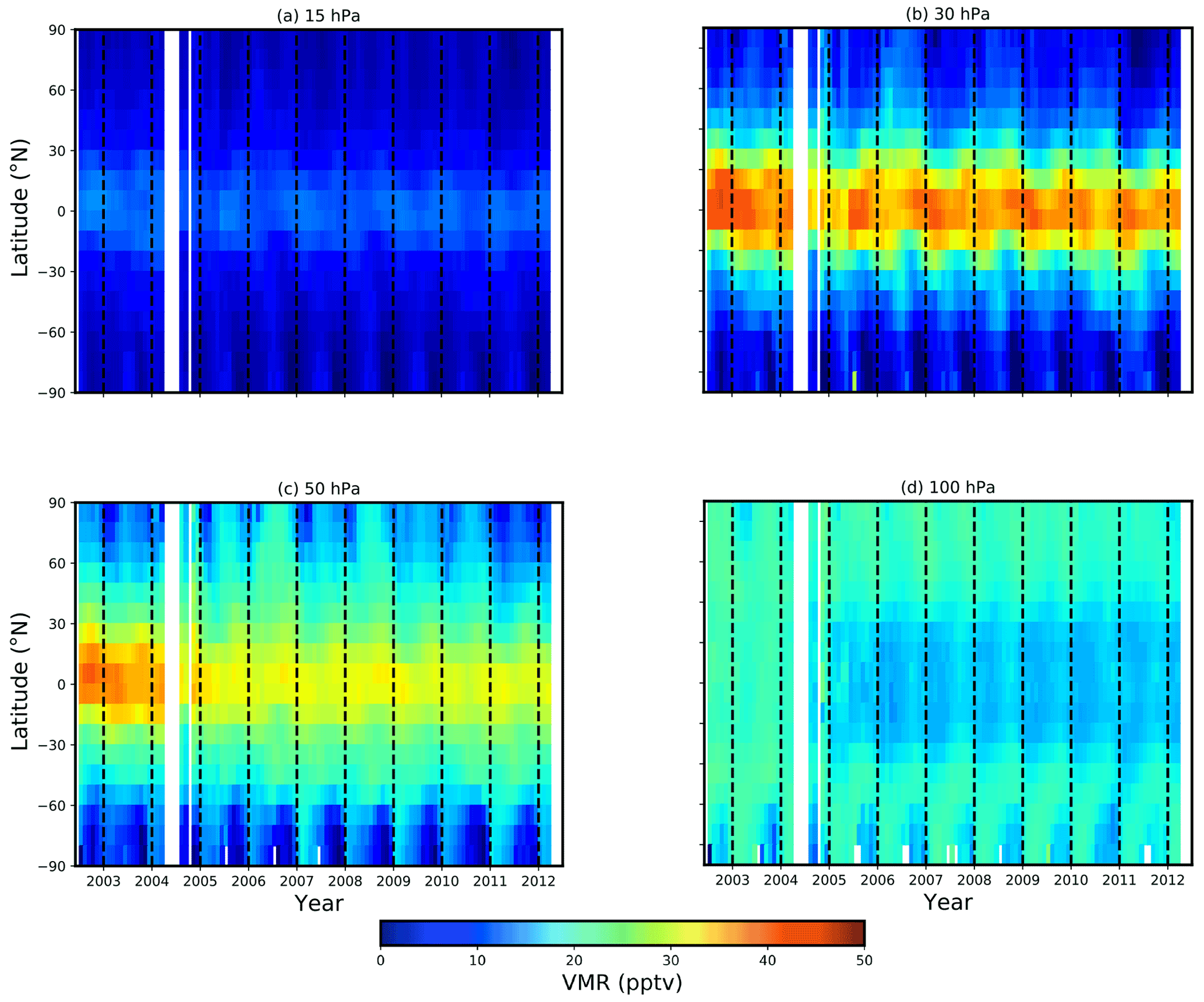
Figure 4Time series of monthly mean COCl2 VMR as a function of latitude (vertical scale). The four panels refer to different pressure levels: 15 hPa (a), 30 hPa (b), 50 hPa (c), and 100 hPa (d). The white areas denote periods of missing measurements. Labels on the x axis indicate the beginning of the years.
The four panels of Fig. 4 illustrate the seasonal and latitudinal variability in the phosgene VMR at four different pressure levels. In general, the seasonal variability is more pronounced in polar regions that are subject to both the largest insolation variability during the year and the presence of a strong vortex during wintertime. At high altitudes (15 hPa), as shown in Fig. 4a, phosgene concentrations are small and rather constant in time, both at the Equator, because of the stable insolation, and at the poles, because at this pressure level CCl4 concentration is very small. Moving downward, down to 50 hPa, the COCl2 VMR increases almost everywhere except at high latitudes during the polar winter. The periodic change in the insolation at the poles originates a COCl2 variability in polar regions, with an alternation between summer peaks and winter deficiencies. The seasonal oscillation becomes less evident at 100 hPa, as shown in Fig. 4d. This is due to the smaller efficiency of the CCl4 photodissociation. An evident offset is present at 50 hPa between FR and OR periods, mainly in the equatorial region. The main reason is the use of different MWs, as shown in Table 1. Other contributions are also due to different vertical resolutions and measurement vertical steps.
To the best of our knowledge, the only available COCl2 measurements that cover the time period of the ENVISAT mission are those of the Atmospheric Chemistry Experiment – Fourier Transform Spectrometer (ACE-FTS) and those of the balloon version of the MIPAS instrument (MIPAS-B). In this section we show the results of the comparison of our products with these measurements.
4.1 Comparison to ACE-FTS
ACE-FTS is a Fourier transform spectrometer on board the SCISAT-1 satellite, launched in August 2003. Starting from February 2004, ACE-FTS has been acquiring solar occultation measurements in the middle infrared (Bernath et al., 2005; Bernath, 2017). From these spectral absorption measurements it is possible to infer the vertical distribution of many atmospheric constituents (Hase et al., 2010). For this intercomparison exercise, we use ACE-FTS v3.5 COCl2 products (Koo et al., 2017), retrieved using the spectroscopic database described in Brown et al. (1996) for COCl2.
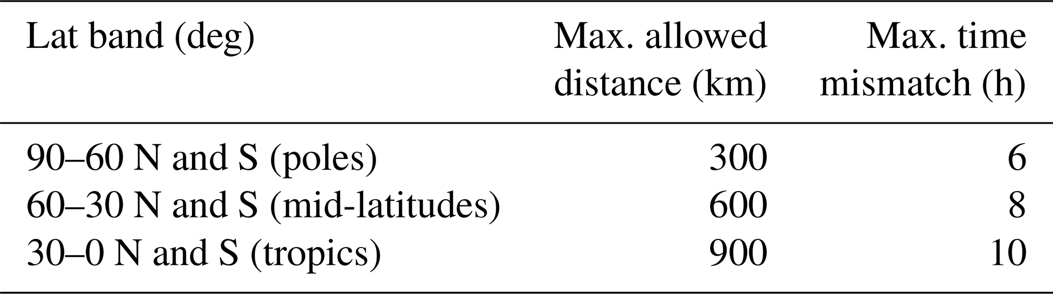
Due to the solar occultation technique, ACE-FTS measurements are quite dense near the poles and sparse in the equatorial regions. For this reason, to have a distribution of co-located measurements as homogeneous as possible all over the globe, latitude-dependent matching criteria have to be used. After some tuning, we adopted the matching criteria described in Table 2. We verified that if more stringent criteria are used, the conclusions of the intercomparison to ACE measurements will not change.
Table 2Latitude-dependent matching criteria used for the intercomparisons with ACE-FTS measurements.
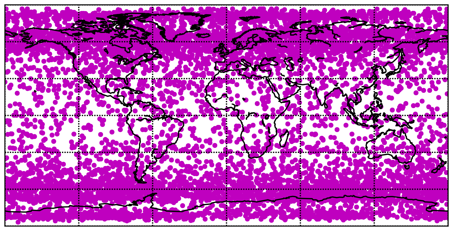
This choice provides 8445 matching measurements distributed as shown in Fig. 5, allowing us to perform a statistically significant intercomparison in all the relevant latitude bands. Note, however, that the number of coincidences in the tropical region is still significantly smaller than at polar and middle latitudes.
First, we interpolated the matching COCl2 profiles to a fixed altitude grid made of the following 14 levels: 9, 10, 11, 12.5, 14, 15.5, 17, 18.5, 20, 21.5, 23, 24.5, 26, and 27.5 km. We then computed the median and the mean of the profile differences for the three latitudinal bands indicated in Table 2. The results are illustrated in Fig. 6.
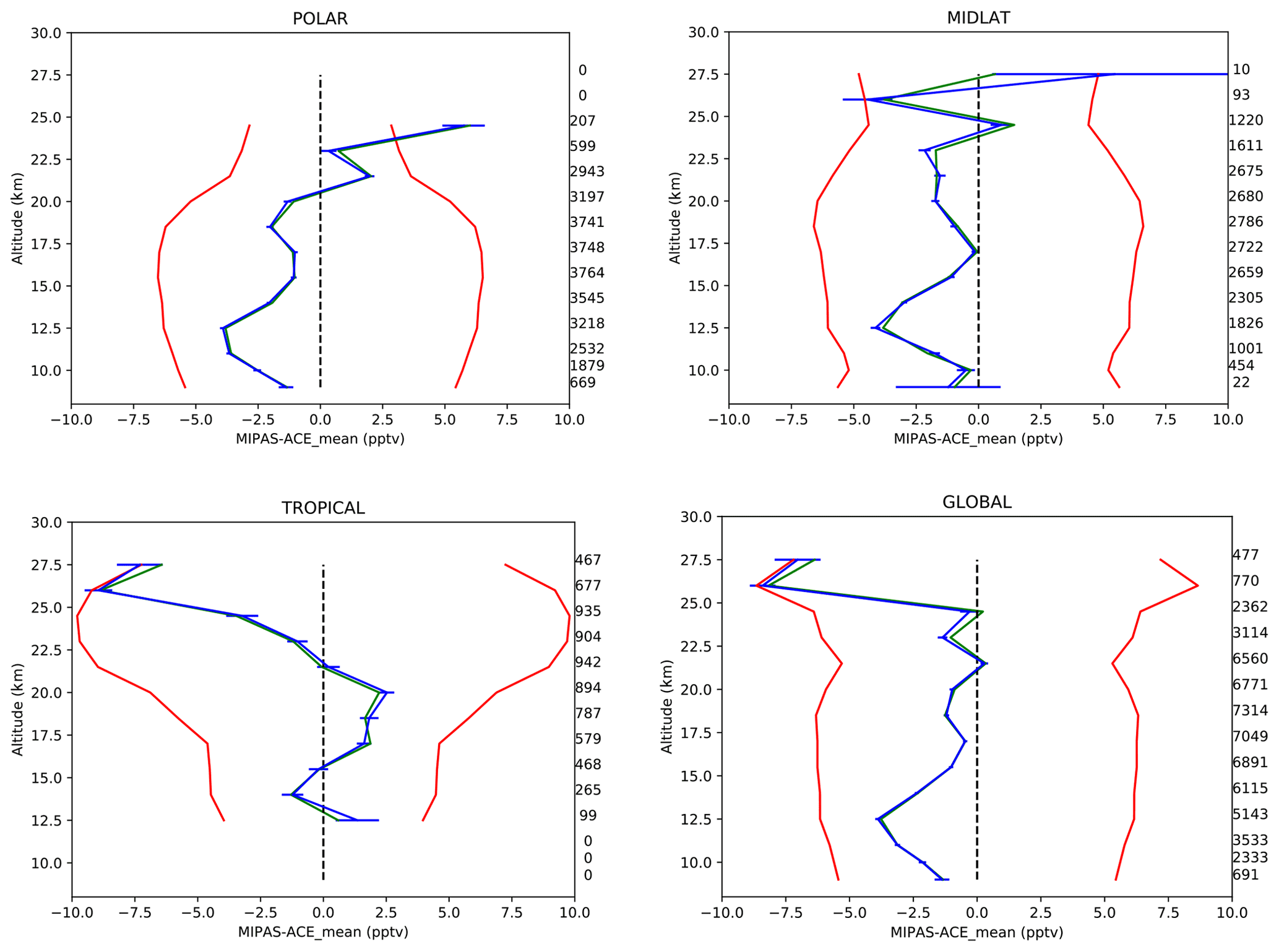
Figure 6Average differences (blue) between MIPAS and ACE-FTS COCl2 profiles for several latitude bands (see plot's key). The median differences are shown in green. Blue bars and red lines represent the random and systematic combined error components, respectively. The number of matching measurements is indicated on the right-hand axis.
Figure 6 shows the average (blue) and median (green) differences between MIPAS and ACE-FTS COCl2 profiles. The blue error bars represent the total random error of the average differences, while the red curves represent the plus/minus combined systematic error bounds. The total systematic error of the average differences was computed as the quadratic summation of MIPAS and ACE-FTS systematic errors. For MIPAS systematic errors, we assumed only the contributions from “spcdb”, “lut”, and “gain-a” as described in Sect. 2. The assumed systematic error on ACE-FTS profiles is 30 %, as suggested in Fu et al. (2007). The combined random error is estimated as the standard deviation of the profile differences divided by the square root of the number of matching measurements.
We see that MIPAS systematically underestimates ACE-FTS in polar and middle latitudes at almost all altitudes. On average, the negative bias is generally smaller than 2 pptv, with the exception of the altitudes around the upper-troposphere–lower-stratosphere, where the negative difference peaks to almost 4 pptv. On the other hand, the equatorial mean differences oscillate around zero, changing from positive values smaller than 2 pptv at about 18 km to negative values, decreasing with altitude, down to about −7 pptv at 26 km. Note that the observed systematic differences are mostly comparable to the estimated systematic errors; therefore, the MIPAS phosgene profiles have a satisfactory agreement with the ACE-FTS ones. It is important to note that the discrepancy with ACE-FTS at high altitudes is not observed in the comparison between MIPAS–ENVISAT (MIPAS-E) and MIPAS balloon (MIPAS-B) (see Fig. 8 in the next section). Part of the systematic differences between MIPAS-E and ACE-FTS can be ascribed to the different spectroscopic databases used in the analysis. Indeed, the analysis of ACE-FTS was performed with the COCl2 spectroscopic database from Brown et al. (1996), while the MIPAS-E analysis uses the newer spectroscopic database (Tchana et al., 2015; Gordon et al., 2017). Figure 7 shows the average difference between COCl2 profiles retrieved with ORM v8 using the two different spectroscopic databases. Some features of these differences are similar to those observed in the intercomparison of Fig. 6. Specifically, we refer to the negative bias in polar regions, and to the shape of the difference profile in the equatorial regions. Another contribution to the bias comes from the different vertical resolutions between MIPAS and ACE; indeed the vertical resolution of ACE profiles is about 3 km, while MIPAS resolution in the OR period (the period considered for this comparison) is about 3.5 km below the altitude of 15 km and degrades with height, reaching the vertical resolution of 10 km at the altitude of 25 km. Since the two vertical resolutions are almost equivalent below 15 km, this effect does not affect the bias at lower altitudes. On the other hand, it can produce a bias above 15 km and in particular a negative bias around the COCl2 peak. Finally, the negative bias that MIPAS profiles have with respect to ACE-FTS ones should not be exclusively regarded as a deficiency in MIPAS data. Indeed, while comparing the upper tropospheric ACE-FTS COCl2 to the chemical transport model TOMCAT (Monks et al., 2017), Harrison et al. (2019) found a positive bias of 10–20 pptv between measurements and model, while the results of the present intercomparison hint to a slightly smaller bias between MIPAS and TOMCAT concentrations. However, the inconsistency is still not completely solved.
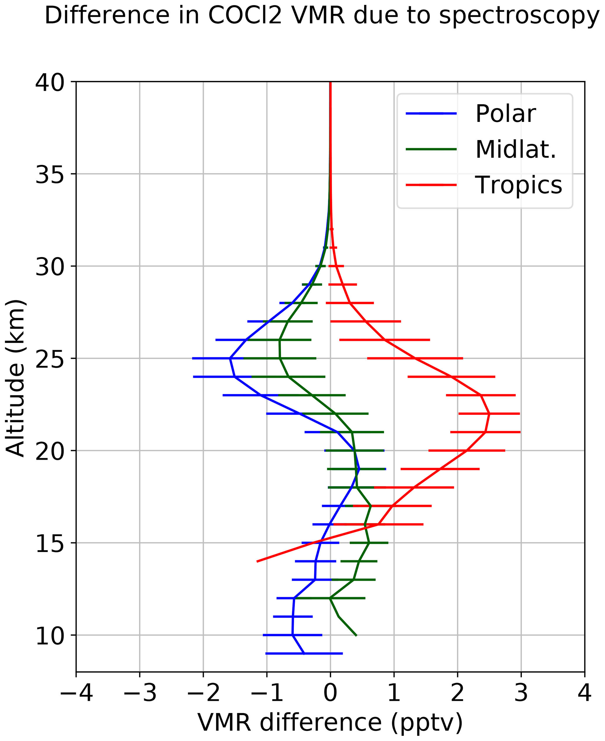
Figure 7Average differences between COCl2 retrieved by ORM v8 using the spectroscopic database described in Gordon et al. (2017) and in Brown et al. (1996). The average was computed using the scans of one orbit of OR measurements, grouped into three latitude bands as described in the label of the figure. The error bars are the errors of the average.
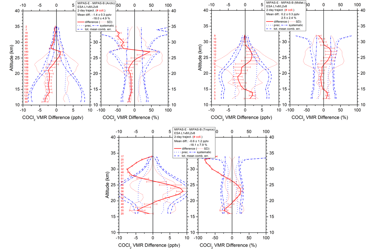
Figure 8Average differences between MIPAS-E and MIPAS-B (Wetzel et al., 2018). The plots show the absolute (left) and relative (right) VMR mean differences between MIPAS-E and MIPAS-B (solid red line) for the match collocations found (red numbers). The standard deviation of the mean and standard deviation of the differences are represented by the error bars and the dotted red lines, respectively. The other curves displayed are systematic (dash-dotted blue lines), precision (dotted blue lines), and total combined errors (dashed blue lines) obtained by adding the errors in quadrature.
4.2 Comparison to MIPAS balloon
The MIPAS-E phosgene profiles have been compared also to MIPAS-B (Wetzel et al., 2018) measurements. Since the balloon-borne sounder MIPAS-B has a number of instrumental characteristics similar to MIPAS-E, like the spectral coverage (750–2500 cm−1) and the spectral resolution (0.0345 cm−1), it can be considered as its precursor. However, the radiometric (NESR) and pointing performances of MIPAS-B are superior. In particular, the error of the tangent altitude is reduced to 90 m (3σ) thanks to the new line-of-sight stabilization. Also the MIPAS-B NESR is improved by computing the average of several spectra acquired at the same elevation angle. Generally, every measurement of a MIPAS-B scan is recorded every 1.5 km of vertical tangent altitude, with a vertical resolution between 3 and 4 km, which is insofar consistent with the ACE's one. The least squares fitting algorithm used to retrieve all the species, on a 1 km grid, is based on analytical derivative spectra computed by the Karlsruhe Optimized and Precise Radiative transfer Algorithm (KOPRA) (Höpfner et al., 1998; Stiller et al., 2002). A regularization approach constrains the difference between the first derivative of the retrieved and an a priori profile in order to avoid retrieval instabilities due to the vertical oversampling. The MIPAS-B phosgene retrieval is performed in the spectral interval between 838.8 and 860.0 cm−1. Spectroscopic parameters from both the MIPAS-E dedicated spectroscopic database (Raspollini et al., 2013; Perrin et al., 2016) and the HITRAN 2008 database (Rothman et al., 2009) are used to simulate the infrared emission spectra. For the COCl2 spectroscopic database, data from Brown et al. (1996) are used. All the details regarding the MIPAS-B error estimation and data analysis can be found in Wetzel et al. (2018). The intercomparison with MIPAS-E is performed using the MIPAS-B flights listed in Table 3. For the intercomparison, both direct matches and trajectory matches are considered. Direct matches occur when both instruments sound the same air mass simultaneously. In the case of trajectory matches, forward and backward trajectories were calculated by the Free University of Berlin (Naujokat and Grunow, 2003) from the balloon measurement geolocation in order to look for air masses observed by MIPAS-E.
Table 3Overview of MIPAS-B flights used for intercomparison with MIPAS–ENVISAT.
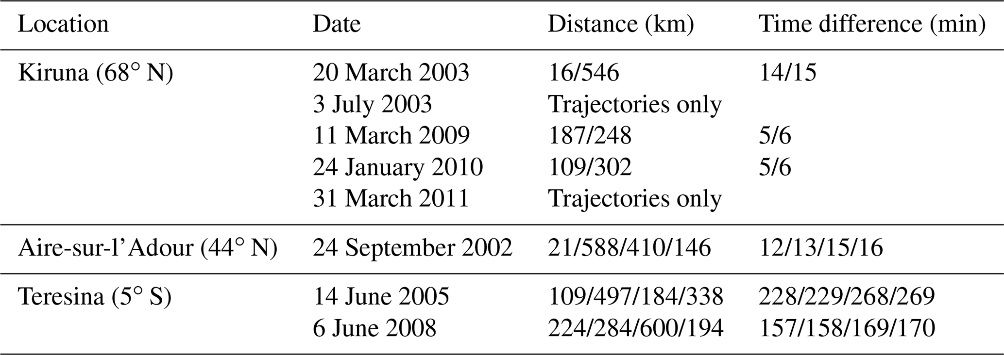
The coincidence criterion, adopted for the identification of both direct and trajectory matches, was of 1 h and 500 km. For a direct comparison to the MIPAS-B data, the MIPAS-E VMR and temperature profiles were interpolated to the altitudes relative to the trajectory matches.
The results in Fig. 8 indicate that MIPAS-E profiles are generally underestimated for arctic and mid-latitude atmospheric conditions with respect to MIPAS-B. In the tropics, the differences oscillate around zero, MIPAS-E being overestimated in the lower-stratosphere–upper-troposphere and underestimated below and above.
Despite some systematic differences, the consistency between the two MIPAS instruments is good; indeed the mean differences, with their error bars, are smaller than the estimated systematic errors almost everywhere. Some exceptions occur at high altitudes.
The behavior of the differences between MIPAS-E and MIPAS-B is still similar to the one obtained in the comparison between MIPAS-E and ACE-FTS presented in Fig. 6, although the amplitude of the differences and the location of the maxima are in some cases different. As already mentioned, the retrievals from both ACE-FTS and MIPAS-B are performed with the COCl2 spectroscopic database from Brown et al. (1996), while MIPAS-E retrievals use data from Tchana et al. (2015). Therefore, we can safely say that part of the differences between MIPAS-E and MIPAS-B are due to the different spectroscopic data used.
To compute COCl2 trends we use the algorithm developed by Valeri et al. (2017). For each pressure level and latitude bin mentioned in Sect. 3, a model VMR(t) is adapted, with the least squares approach, to the time series of the monthly COCl2 averages. As explained in Valeri et al. (2017), the model includes two different offsets for the two mission phases (FR and OR), a common linear term (the trend we are interested in), quasi-biennial-oscillation- and solar-flux-related terms, and the characteristic atmospheric periodicities of 24, 18, 12, 9, 8, 6, 4, and 3 months.
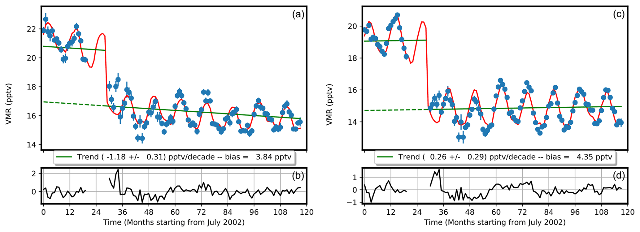
Figure 9Blue dots are the monthly average VMRs with their error bars. The VMR(t) model and the linear term are represented by the red curve and the green line, respectively, with two different intercepts for the FR and the OR mission phases. The trend is the slope of the green lines. Panels (a) and (b) refer to the latitude bin centered at 15∘ N at the pressure level of 100 hPa, and panels (c) and (d) refer to 25∘ S and 115 hPa. The black lines in (b) and (d) show the residuals of the fits.
Figure 9 illustrates the behavior of the fit of the monthly averages for two specific pressure levels and latitude bins. Figure 9a refers to the latitude bin centered at 15∘ N and the pressure level of 100 hPa, and the right plot refers to 25∘ S and 115 hPa. Blue dots are the monthly mean VMRs with their error bars, computed as the standard deviation of the mean. The VMR(t) model and the linear term are represented by the red curve and the green lines, respectively, with two different offsets for the FR and the OR mission phases. The slope of the green lines represents the linear trend we estimate. The black lines plotted in Fig. 9b and d represent the residuals of the fit, computed as the observed monthly means minus the model VMR(t) values. Note that the residuals oscillate around zero, except in the first half of 2005 (between the 24th and 36th months), which corresponds to the transition period between FR and OR mission phases. The two plots show that the same model VMR(t) used in Valeri et al. (2017) to fit the time series of the CCl4 monthly means is able to properly capture also the COCl2 variability. In the fitting procedure we associate to each monthly mean the standard error of the mean. This error accounts for both the variable error components (see Sect. 2) of the individual measurements that contribute to the average and the temporal and spatial variability in the atmosphere within the considered month and latitude band. Systematic error components such as spectroscopic errors and errors due to lookup-table compression (“lut”) provide a constant contribution during the entire mission; thus they do not affect the trend estimate. A different consideration applies to the radiometric calibration error (“gain-a”) which, due to the detector aging, may drift during the mission and, thus, affect the trend estimate. According to the most recent assessment for the level 1b version 8 products (see Sect. 2 and Kleinert et al., 2007), however, the drift of the calibration error has been estimated to be less than 0.5 % across the whole MIPAS mission. Since the COCl2 error due to the uncertainty in radiometric calibration (“gain-a”, see Fig. 1) on its own is generally smaller than 5 %, its drift can be considered to have a negligible impact on the estimated trends, as compared to the random error.
In summary, we compute the trend error by simply propagating the monthly mean standard error onto the derived trends. To account for the quality of the retrieval, we multiply this number by the square root of the normalized chi-square of the trend fit (i.e., the normalized error-weighted L2 norm of the residuals of the fit).
Figure 10 shows the COCl2 absolute trends (a) and their errors (b). Percentage trends (c) and errors (d), computed as the ratio between their absolute values and the average VMR in the corresponding grid cell, are shown in the same figure. In Fig. 11 we show the inverse of the trends' relative error. This is a quantifier for the statistical significance of the trends themselves. Whenever the computed trend is smaller or of the same order of its error, the trend has little statistical significance and, actually, could be either positive or negative. Values of the inverse relative error greater than 2 or 3 indicate a statistically significant trend. Among the determined trends, the ones with the largest statistical significance are located in the Northern Hemisphere.
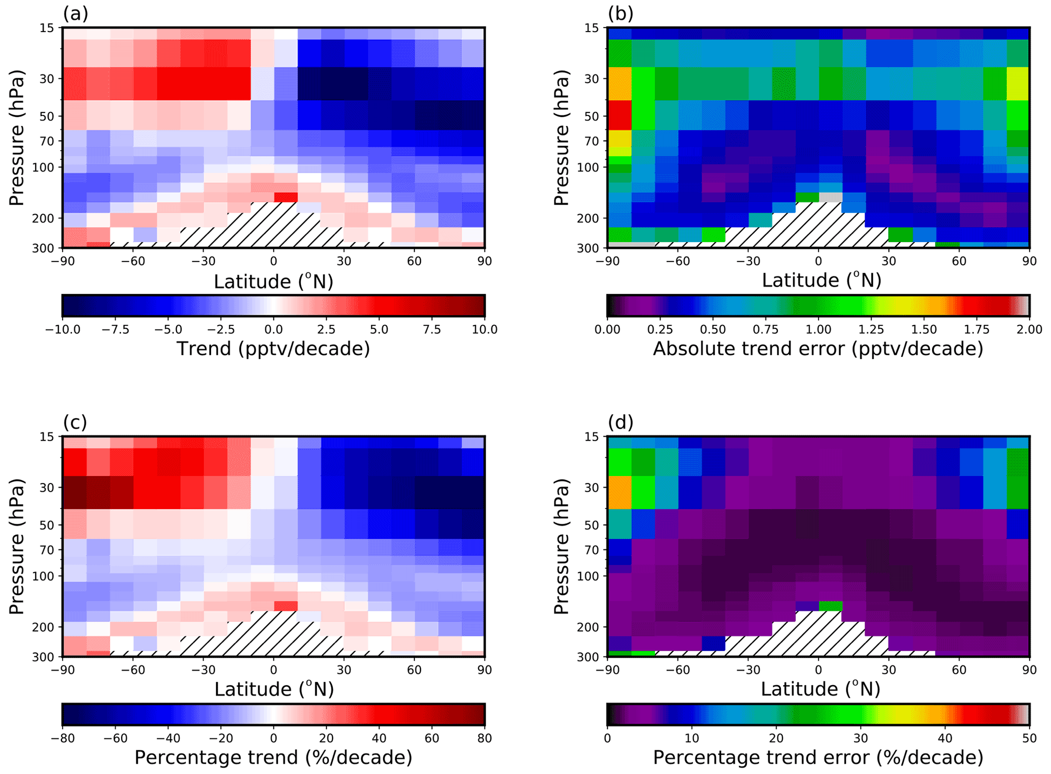
Figure 10Absolute (a) and percentage (c) COCl2 trends for each latitude and pressure bin. Absolute and percentage trend errors are reported in panels (b) and (d), respectively. Dashed areas represent pressure levels and latitude bins with too few data.
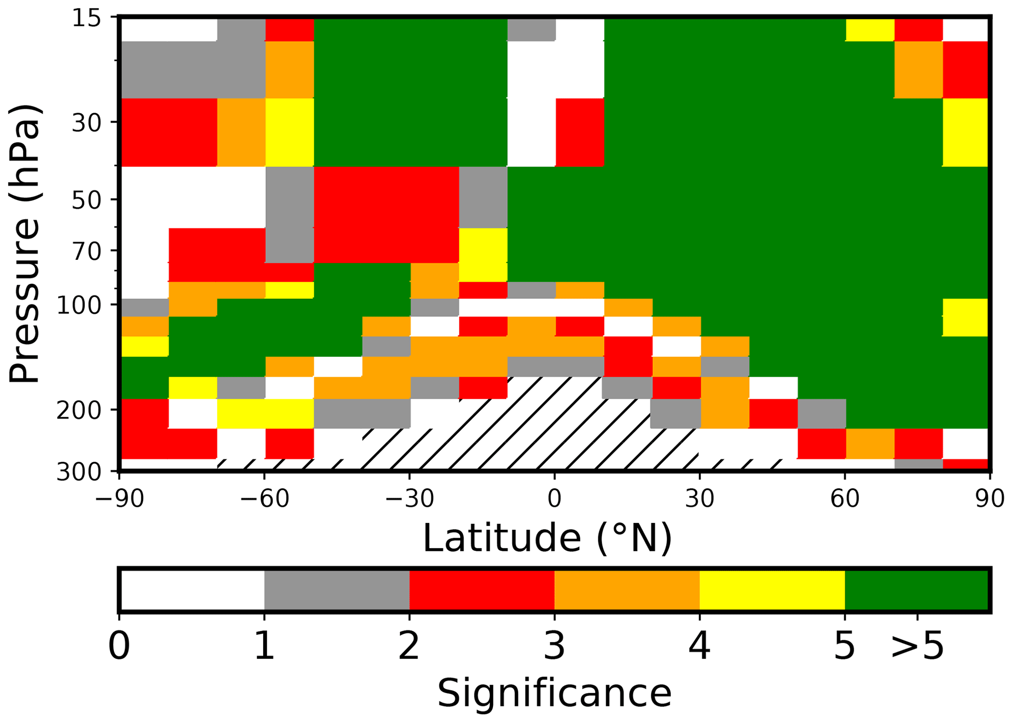
Figure 11Statistical significance (inverse relative error) of the determined trends. Dashed areas represent pressure levels and latitude bins with too few data.
From Fig. 10 we see that negative trends characterize the stratosphere in the Northern Hemisphere with values down to −7 pptv per decade at 30 hPa. In the Southern Hemisphere the trend values range from negative (about −2 pptv per decade) for pressures between 200 and 70 hPa to positive (about 4 pptv per decade) above 50 hPa. At high altitudes there is an evident asymmetry between the Northern Hemisphere and Southern Hemisphere. In the upper troposphere we find a positive trend in both hemispheres even if its statistical significance (see Fig. 11) is smaller than in the stratosphere.
A similar analysis of COCl2 trends resolved in latitude and altitude has recently been published by Harrison et al. (2019). In that work, phosgene trends based on ACE-FTS measurements and on the TOMCAT/SLIMCAT model (Chipperfield, 2006) were derived for the period from January 2004 to December 2016. The trends from ACE-FTS measurements were computed from monthly percentage anomalies in COCl2 zonal means. The authors did not include additional terms such as the annual cycle and its harmonics, claiming that they cause no additional improvements in the regression. The map of the trends versus pressure and latitude derived from MIPAS ESA v8 products is consistent with the results from both ACE-FTS measurements and TOMCAT simulations, i.e., the negative trend in the lower stratosphere in both hemispheres, the trend asymmetry in the two hemispheres in the middle stratosphere, and the positive trend in the upper troposphere. In particular the latter, attributed by Harrison et al. (2019) to the increase in Cl-containing VSLSs, confirms the importance of COCl2 as a marker for Cl-containing VSLSs.
In their paper, Harrison et al. (2019) also computed the overall VMR-weighted trend from both ACE measurements and TOMCAT simulations. This parameter is calculated as the average of the trends at all latitude and altitude bins, weighted with the mean VMR in each bin. The results of Harrison et al. (2019) are pptv yr−1 for the trend from ACE data and pptv yr−1 for the trend from the TOMCAT model. To compare more quantitatively MIPAS and ACE-FTS trends we also computed from our MIPAS trends an overall VMR-weighted trend with the same procedure. We get pptv yr−1, in which the error has been estimated by propagating the errors of each individual trend and monthly mean VMR. Although ACE-FTS and TOMCAT overall trends are not self-consistent, the MIPAS result falls within these two values at a distance of 2.5 to 3σ from them.
Concerning the trend asymmetry in the upper stratosphere, a similar feature has been also observed for (Kellmann et al., 2012), and CCl4 (Valeri et al., 2017) trends. According to some recent research (Harrison et al., 2019; Mahieu et al., 2014; Ploeger et al., 2015), the stratospheric circulation variability is able to affect the stratospheric trends of several halogen source gases and the derived compounds, i.e., HF and HCl. Such results give a partial explanation as to why the stratospheric trend does not always resemble the tropospheric one with a time lag.
The production of atmospheric phosgene is mainly due to the chlorocarbon compounds' decomposition, primarily CCl4 and, secondarily, CH3CCl3 and VSLSs. In this study, the global vertical distribution of upper tropospheric and lower and middle stratospheric COCl2, retrieved by the ESA level 2 v8 processor (ORM v8) from the full set of MIPAS-E measurements in the decade 2002–2012, is reported. We find peak values of phosgene of the order of ≈40 pptv in the tropical lower stratosphere. This is the latitude and altitude where both sun insolation and CCl4 VMR (a species of anthropogenic origin and whose concentration decreases with altitude) are high enough to trigger COCl2 production. Minimum values, approaching 0 pptv, are found between 15 and 30 hPa over polar regions, where both insolation and CCl4 VMR are scarce.
Intercomparisons of MIPAS phosgene profiles with ACE-FTS and MIPAS-B measurements reveal a slight negative bias of MIPAS at polar and middle latitudes of the order of 2 pptv. Analyzing both MIPAS-B and ACE intercomparisons, we can say that part of the bias is due to the fact that the retrieval of MIPAS-E measurements uses the most recent COCl2 spectroscopic database (Tchana et al., 2015; Gordon et al., 2017).
For the computation of the trends, we interpolated the MIPAS phosgene profiles retrieved at fixed pressure levels and grouped them into 10∘ latitude bins. For each pressure level and latitude bin, we calculated monthly averages for the whole period of the MIPAS mission, from July 2002 to April 2012. By fitting a model to the monthly averages, we determined the COCl2 trends. Negative trends characterize the lowest and middle stratosphere of the Northern Hemisphere with values down to −7 pptv per decade at 30 hPa. In the Southern Hemisphere the trend values range from negative (about −2 pptv per decade) for pressures between 200 and 70 hPa to positive (about 4 pptv per decade) over 70 hPa. In the upper troposphere we find positive trends at all latitudes in both hemispheres. However, such values are never larger than 1 or 2 times their error bars; therefore, their statistical significance is lower than in the stratosphere. A similar tropospheric trend distribution has been found by Harrison et al. (2019) using ACE-FTS measurements. This behavior was attributed to the increase in Cl-containing VSLSs, and so this result confirms the importance of COCl2 as a marker for Cl-containing VSLSs.
As stratospheric COCl2 is primarily generated by the photolysis of CCl4, the stratospheric COCl2 trend is similar to the one of CCl4, which is negative almost everywhere, except in the Southern Hemisphere over 50 hPa where the trend is positive in some regions (Valeri et al., 2017). However, some differences exist. A positive trend in the Southern Hemisphere is more evident for COCl2 where peaks of more than 60 % per decade are present, while CCl4 does not increase more than 30 % per decade and is in a more limited region. Indeed, despite the photolysis of CCl4 being the main stratospheric source of phosgene, other chlorocarbon compounds, like VSLSs, whose stratospheric concentration is increasing (Hossaini et al., 2019), can play an important role. MIPAS COCl2 trend behavior is similar to that found by Harrison et al. (2019) from ACE-FTS results, and both the signs and the asymmetry between the two hemispheres are in good agreement. Regarding the overall VMR-weighted trend values, our result of pptv yr−1 falls right in between the value inferred from ACE of pptv yr−1 and the TOMCAT model estimate of pptv yr−1 (Harrison et al., 2019).
The knowledge of the COCl2 distribution and trend, estimated by MIPAS measurements, can be important to improve the chemical transport models and to better understand the atmospheric sources and sinks of Cl-containing species. This study also provides an independent confirmation, obtained with a better temporal and spatial coverage, of the ACE results. In the future, the continuity of this study will be provided by ACE-FTS measurements, which are still being acquired.
MIPAS ESA level 2 v8 products can be obtained via https://earth.esa.int/eogateway/ (last access: 16 December 2021, European Space Agency, 2021, https://doi.org/10.5270/EN1-c8hgqx4) (registration required). Trend values are available upon request to the authors.
ACE-FTS level 2 version v3.5 products can be obtained via http://www.ace.uwaterloo.ca/data.php (last access: 16 December 2021, Bernath et al., 2021, https://doi.org/10.20383/102.0495) (upon request).
PR, MR, LS, MG, BMD, FB, and SC are the main authors of the MIPAS ESA ORM v8 processor. NZ computed from the MIPAS level 2 v8 products the monthly means that were used to derive the trends and the global distribution maps. MV and MR designed and implemented the algorithm to derive trends. PP computed trends and compared MIPAS COCl2 profiles to ACE-FTS. Comparisons to MIPAS-B measurements were done by GW. PP, PR, and BMD discussed the results. The paper was first drafted by PP and then carefully reviewed by all co-authors. BMD and MR procured funding for the research contract of PP.
The contact author has declared that neither they nor their co-authors have any competing interests.
Publisher's note: Copernicus Publications remains neutral with regard to jurisdictional claims in published maps and institutional affiliations.
This article is part of the special issue “MIPAS ESA Level 2 version 8 products: algorithms, product features and validation”. It is not associated with a conference.
The Atmospheric Chemistry Experiment (ACE), also known as SCISAT, is a Canadian-led mission mainly supported by the Canadian Space Agency.
We thank the MIPAS Quality Working Group for the work done to improve the level 1 and the level 2 processors.
The MIPAS COCl2 VMR dataset was generated as part of the ESA level 2 v8 full mission reprocessing of MIPAS measurements performed under ESA contract no. 4000112093/14/I-LG.
This paper was edited by Martin Riese and reviewed by two anonymous referees.
Bernath, P. F.: The Atmospheric Chemistry Experiment (ACE), J. Quant. Spectrosc. Ra., 186, 3–16, https://doi.org/10.1016/j.jqsrt.2016.04.006, 2017. a
Bernath, P. F., McElroy, C. T., Abrams, M. C., Boone, C. D., Butler, M., Camy-Peyret, C., Carleer, M., Clerbaux, C., Coheur, P.-F., Colin, R., DeCola, P., DeMazière, M., Drummond, J. R., Dufour, D., Evans, W. F. J., Fast, H., Fussen, D., Gilbert, K., Jennings, D. E., Llewellyn, E. J., Lowe, R. P., Mahieu, E., McConnell, J. C., McHugh, M., McLeod, S. D., Michaud, R., Midwinter, C., Nassar, R., Nichitiu, F., Nowlan, C., Rinsland, C. P., Rochon, Y. J., Rowlands, N., Semeniuk, K., Simon, P., Skelton, R., Sloan, J. J., Soucy, M.-A., Strong, K., Tremblay, P., Turnbull, D., Walker, K. A., Walkty, I., Wardle, D. A., Wehrle, V., Zander, R., and Zou, J.: Atmospheric Chemistry Experiment (ACE): Mission overview, Geophys. Res. Lett., 32, L15S01, https://doi.org/10.1029/2005GL022386, 2005. a
Bernath, P., Boone, C., Steffen, J., and Crouse, J.: Atmospheric Chemistry Experiment SciSat Level 2 Processed Data, v3.5/v3.6, Federated Research Data Repository [data set], https://doi.org/10.20383/102.0495, 2021 (data available at: http://www.ace.uwaterloo.ca/data.php, last access: 16 December 2021). a
Bris, K., Pandharpurkar, R., and Strong, K.: Mid-infrared absorption cross-sections and temperature dependence of CFC-113, J. Quant. Spectrosc. Ra., 112, 1280–1285, https://doi.org/10.1016/j.jqsrt.2011.01.023, 2011. a
Brown, L. R., Gunson, M. R., Toth, R. A., Irion, F. W., Rinsland, C. P., and Goldman, A.: 1995 Atmospheric Trace Molecule Spectroscopy (ATMOS) linelist, Appl. Optics, 35, 2828–2848, https://doi.org/10.1364/AO.35.002828, 1996. a, b, c, d, e
Ceccherini, S. and Ridolfi, M.: Technical Note: Variance-covariance matrix and averaging kernels for the Levenberg-Marquardt solution of the retrieval of atmospheric vertical profiles, Atmos. Chem. Phys., 10, 3131–3139, https://doi.org/10.5194/acp-10-3131-2010, 2010. a
Chipperfield, M. P.: New version of the TOMCAT/SLIMCAT off-line chemical transport model: Intercomparison of stratospheric tracer experiments, Q. J. Roy. Meteor. Soc., 132, 1179–1203, https://doi.org/10.1256/qj.05.51, 2006. a
Dinelli, B. M., Arnone, E., Brizzi, G., Carlotti, M., Castelli, E., Magnani, L., Papandrea, E., Prevedelli, M., and Ridolfi, M.: The MIPAS2D database of MIPAS/ENVISAT measurements retrieved with a multi-target 2-dimensional tomographic approach, Atmos. Meas. Tech., 3, 355–374, https://doi.org/10.5194/amt-3-355-2010, 2010. a
Dinelli, B. M., Raspollini, P., Gai, M., Sgheri, L., Ridolfi, M., Ceccherini, S., Barbara, F., Zoppetti, N., Castelli, E., Papandrea, E., Pettinari, P., Dehn, A., Dudhia, A., Kiefer, M., Piro, A., Flaud, J.-M., Lopez-Puertas, M., Moore, D., Remedios, J., and Bianchini, M.: The ESA MIPAS/ENVISAT Level2-v8 dataset: 10 years of measurements retrieved with ORM v8.22, Atmos. Meas. Tech. Discuss. [preprint], https://doi.org/10.5194/amt-2021-215, in review, 2021. a, b, c, d
Dudhia, A.: MIPAS L2 Error Analyses, available at: http://eodg.atm.ox.ac.uk/MIPAS/err/ (last access: 16 December 2021), 2019. a, b, c
Dudhia, A., L Jay, V., and D Rodgers, C.: Microwindow Selection for High-Spectral-Resolution Sounders, Appl. Optics, 41, 3665–3673, https://doi.org/10.1364/AO.41.003665, 2002. a
Engel, A. and Rigby, M.: Chapter 1: Update on Ozone Depleting Substances (ODSs) and Other Gases of Interest to the Montreal Protocol, in: Global Ozone Research and Monitoring Project, vol. 58, World Meteorological Organization Technical Document, 2019. a, b
European Space Agency: Envisat MIPAS L2 – Temperature, Pressure and Atmospheric Constituents Profiles Product, Version 8.22, ESA [data set], https://doi.org/10.5270/EN1-c8hgqx4, 2021. a
Fischer, H., Birk, M., Blom, C., Carli, B., Carlotti, M., von Clarmann, T., Delbouille, L., Dudhia, A., Ehhalt, D., Endemann, M., Flaud, J. M., Gessner, R., Kleinert, A., Koopman, R., Langen, J., López-Puertas, M., Mosner, P., Nett, H., Oelhaf, H., Perron, G., Remedios, J., Ridolfi, M., Stiller, G., and Zander, R.: MIPAS: an instrument for atmospheric and climate research, Atmos. Chem. Phys., 8, 2151–2188, https://doi.org/10.5194/acp-8-2151-2008, 2008. a
Fitzgerald, G.: Chemical warfare and medical response during World War I, Am. J. Public Health, 98, 611–625, 2008. a
Fu, D., D. Boone, C., F. Bernath, P., A. Walker, K., Nassar, R., Manney, G., and D. McLeod, S.: Global phosgene observations from the Atmospheric Chemistry Experiment (ACE) mission, Geophys. Res. Lett., 34, L17815, https://doi.org/10.1029/2007GL029942, 2007. a, b
Gordon, I., Rothman, L., Hill, C., Kochanov, R., Tan, Y., Bernath, P., Birk, M., Boudon, V., Campargue, A., Chance, K., Drouin, B., Flaud, J.-M., Gamache, R., Hodges, J., Jacquemart, D., Perevalov, V., Perrin, A., Shine, K., Smith, M.-A., Tennyson, J., Toon, G., Tran, H., Tyuterev, V., Barbe, A., Császár, A., Devi, V., Furtenbacher, T., Harrison, J., Hartmann, J.-M., Jolly, A., Johnson, T., Karman, T., Kleiner, I., Kyuberis, A., Loos, J., Lyulin, O., Massie, S., Mikhailenko, S., Moazzen-Ahmadi, N., Müller, H., Naumenko, O., Nikitin, A., Polyansky, O., Rey, M., Rotger, M., Sharpe, S., Sung, K., Starikova, E., Tashkun, S., Auwera, J. V., Wagner, G., Wilzewski, J., Wcisło, P., Yu, S., and Zak, E.: The HITRAN2016 molecular spectroscopic database, J. Quant. Spectrosc. Ra., 203, 3–69, https://doi.org/10.1016/j.jqsrt.2017.06.038, hITRAN2016 Special Issue, 2017. a, b, c, d, e
Harrison, J. J.: New and improved infrared absorption cross sections for trichlorofluoromethane (CFC-11), Atmos. Meas. Tech., 11, 5827–5836, https://doi.org/10.5194/amt-11-5827-2018, 2018. a
Harrison, J. J., Chipperfield, M. P., Hossaini, R., Boone, C. D., Dhomse, S., Feng, W., and Bernath, P. F.: Phosgene in the Upper Troposphere and Lower Stratosphere: A Marker for Product Gas Injection Due to Chlorine-Containing Very Short Lived Substances, Geophys. Res. Lett., 46, 1032–1039, https://doi.org/10.1029/2018GL079784, 2019. a, b, c, d, e, f, g, h, i, j, k
Hase, F., Wallace, L., D. McLeod, S., Harrison, J., and F. Bernath, P.: The ACE-FTS atlas of the infrared solar spectrum, J. Quant. Spectrosc. Ra., 111, 521–528, https://doi.org/10.1016/j.jqsrt.2009.10.020, 2010. a
Hegglin, M. I., Tegtmeier, S., Anderson, J., Froidevaux, L., Fuller, R., Funke, B., Jones, A., Lingenfelser, G., Lumpe, J., Pendlebury, D., Remsberg, E., Rozanov, A., Toohey, M., Urban, J., von Clarmann, T., Walker, K. A., Wang, R., and Weigel, K.: SPARC Data Initiative: Comparison of water vapor climatologies from international satellite limb sounders, J. Geophys. Res.-Atmos., 118, 11824–11846, https://doi.org/10.1002/jgrd.50752, 2013. a
Hossaini, R., Atlas, E., Dhomse, S. S., Chipperfield, M. P., Bernath, P. F., Fernando, A. M., Mühle, J., Leeson, A. A., Montzka, S. A., Feng, W., Harrison, J. J., Krummel, P., Vollmer, M. K., Reimann, S., O'Doherty, S., Young, D., Maione, M., Arduini, J., and Lunder, C. R.: Recent Trends in Stratospheric Chlorine From Very Short-Lived Substances, J. Geophys. Res.-Atmos., 124, 2318–2335, https://doi.org/10.1029/2018JD029400, 2019. a
Höpfner, M., P. Stiller, G., Kuntz, M., Clarmann von, T., Echle, G., Funke, B., Glatthor, N., Hase, F., Kemnitzer, H., and Zorn, S.: The Karlsruhe optimized and precise radiative transfer algorithm. Part II. Interface to retrieval applications, Optical Remote Sensing of the Atmosphere and Clouds, 3501, 187–195, https://doi.org/10.1117/12.317753, 1998. a
Kellmann, S., von Clarmann, T., Stiller, G. P., Eckert, E., Glatthor, N., Höpfner, M., Kiefer, M., Orphal, J., Funke, B., Grabowski, U., Linden, A., Dutton, G. S., and Elkins, J. W.: Global CFC-11 (CCl3F) and CFC-12 (CCl2F2) measurements with the Michelson Interferometer for Passive Atmospheric Sounding (MIPAS): retrieval, climatologies and trends, Atmos. Chem. Phys., 12, 11857–11875, https://doi.org/10.5194/acp-12-11857-2012, 2012. a
Kindler, T. P., Chameides, W. L., Wine, P. H., Cunnold, D. M., Alyea, F. N., and Franklin, J. A.: The fate of atmospheric phosgene and the stratospheric chlorine loadings of its parent compounds: CCl4, C2Cl4, C2HCl3, CH3CCl3, and CHCl3, J. Geophys. Res.-Atmos., 100, 1235–1251, https://doi.org/10.1029/94JD02518, 1995. a
Kleinert, A., Aubertin, G., Perron, G., Birk, M., Wagner, G., Hase, F., Nett, H., and Poulin, R.: MIPAS Level 1B algorithms overview: operational processing and characterization, Atmos. Chem. Phys., 7, 1395–1406, https://doi.org/10.5194/acp-7-1395-2007, 2007. a, b
Kleinert, A., Birk, M., Perron, G., and Wagner, G.: Level 1b error budget for MIPAS on ENVISAT, Atmos. Meas. Tech., 11, 5657–5672, https://doi.org/10.5194/amt-11-5657-2018, 2018. a, b
Koo, J.-H., Walker, K. A., Jones, A., Sheese, P. E., Boone, C. D., Bernath, P. F., and Manney, G. L.: Global climatology based on the ACE-FTS version 3.5 dataset: Addition of mesospheric levels and carbon-containing species in the UTLS, J. Quant. Spectrosc. Ra., 186, 52–62, https://doi.org/10.1016/j.jqsrt.2016.07.003, 2017. a
Mahieu, E., Chipperfield, M. P., Notholt, J., Reddmann, T., Anderson, J. J., Bernath, P. F., Blumenstock, T., Coffey, M. T., Dhomse, S. S., Feng, W., Franco, B., Froidevaux, L., Griffith, D. W. T., Hannigan, J. W., Hase, F., Hossaini, R., Jones, N. G. B., Morino, I., Murata, I., Nakajima, H., Palm, M., Paton-Walsh, C., Russell, J. M., Schneider, M., Stiller, G. P., Smale, D. A., and Walker, K. A.: Recent Northern Hemisphere stratospheric HCl increase due to atmospheric circulation changes, Nature, 515, 104–107, 2014. a
Monks, S. A., Arnold, S. R., Hollaway, M. J., Pope, R. J., Wilson, C., Feng, W., Emmerson, K. M., Kerridge, B. J., Latter, B. L., Miles, G. M., Siddans, R., and Chipperfield, M. P.: The TOMCAT global chemical transport model v1.6: description of chemical mechanism and model evaluation, Geosci. Model Dev., 10, 3025–3057, https://doi.org/10.5194/gmd-10-3025-2017, 2017. a
Naujokat, B. and Grunow, K.: The stratospheric Arctic winter 2002/03: balloon flight planning by trajectory calculations, European Space Agency, (Special Publication) ESA SP, 530, 421–425, 2003. a
Perrin, A., Flaud, J.-M., Ridolfi, M., Vander Auwera, J., and Carlotti, M.: MIPAS database: new HNO3 line parameters at 7.6 µm validated with MIPAS satellite measurements, Atmos. Meas. Tech., 9, 2067–2076, https://doi.org/10.5194/amt-9-2067-2016, 2016. a, b
Ploeger, F., Riese, M., Haenel, F., Konopka, P., Müller, R., and Stiller, G.: Variability of stratospheric mean age of air and of the local effects of residual circulation and eddy mixing, J. Geophys. Res.-Atmos., 120, 716–733, https://doi.org/10.1002/2014JD022468, 2015. a
Raspollini, P., Belotti, C., Burgess, A., Carli, B., Carlotti, M., Ceccherini, S., Dinelli, B. M., Dudhia, A., Flaud, J.-M., Funke, B., Höpfner, M., López-Puertas, M., Payne, V., Piccolo, C., Remedios, J. J., Ridolfi, M., and Spang, R.: MIPAS level 2 operational analysis, Atmos. Chem. Phys., 6, 5605–5630, https://doi.org/10.5194/acp-6-5605-2006, 2006. a
Raspollini, P., Carli, B., Carlotti, M., Ceccherini, S., Dehn, A., Dinelli, B. M., Dudhia, A., Flaud, J.-M., López-Puertas, M., Niro, F., Remedios, J. J., Ridolfi, M., Sembhi, H., Sgheri, L., and von Clarmann, T.: Ten years of MIPAS measurements with ESA Level 2 processor V6 – Part 1: Retrieval algorithm and diagnostics of the products, Atmos. Meas. Tech., 6, 2419–2439, https://doi.org/10.5194/amt-6-2419-2013, 2013. a, b, c
Raspollini, P., Arnone, E., Barbara, F., Bianchini, M., Carli, B., Ceccherini, S., Chipperfield, M. P., Dehn, A., Della Fera, S., Dinelli, B. M., Dudhia, A., Flaud, J.-M., Gai, M., Kiefer, M., López-Puertas, M., Moore, D. P., Piro, A., Remedios, J. J., Ridolfi, M., Sembhi, H., Sgheri, L., and Zoppetti, N.: Level 2 processor and auxiliary data for ESA Version 8 final full mission analysis of MIPAS measurements on ENVISAT, Atmos. Meas. Tech. Discuss. [preprint], https://doi.org/10.5194/amt-2021-235, in review, 2021. a, b, c, d, e, f
Remedios, J. J., Leigh, R. J., Waterfall, A. M., Moore, D. P., Sembhi, H., Parkes, I., Greenhough, J., Chipperfield, M. P., and Hauglustaine, D.: MIPAS reference atmospheres and comparisons to V4.61/V4.62 MIPAS level 2 geophysical data sets, Atmos. Chem. Phys. Discuss., 7, 9973–10017, https://doi.org/10.5194/acpd-7-9973-2007, 2007. a
Ridolfi, M. and Sgheri, L.: A self-adapting and altitude-dependent regularization method for atmospheric profile retrievals, Atmos. Chem. Phys., 9, 1883–1897, https://doi.org/10.5194/acp-9-1883-2009, 2009. a
Ridolfi, M., Carli, B., Carlotti, M., von Clarmann, T., Dinelli, B. M., Dudhia, A., Flaud, J.-M., Höpfner, M., Morris, P. E., Raspollini, P., Stiller, G., and Wells, R. J.: Optimized forward model and retrieval scheme for MIPAS near-real-time dataprocessing, Appl. Optics, 39, 1323–1340, https://doi.org/10.1364/AO.39.001323, 2000. a
Rodgers, C. D.: Inverse methods for atmospheric sounding: theory and practice, World Scientific Book, https://doi.org/10.1142/3171, 2000. a, b
Rothman, L., Gordon, I., Barbe, A., Benner, D., Bernath, P., Birk, M., Boudon, V., Brown, L., Campargue, A., Champion, J.-P., Chance, K., Coudert, L., Dana, V., Devi, V., Fally, S., Flaud, J.-M., Gamache, R., Goldman, A., Jacquemart, D., Kleiner, I., Lacome, N., Lafferty, W., Mandin, J.-Y., Massie, S., Mikhailenko, S., Miller, C., Moazzen-Ahmadi, N., Naumenko, O., Nikitin, A., Orphal, J., Perevalov, V., Perrin, A., Predoi-Cross, A., Rinsland, C., Rotger, M., Šimeçková, M., Smith, M., Sung, K., Tashkun, S., Tennyson, J., Toth, R., Vandaele, A., and Auwera, J. V.: The HITRAN 2008 molecular spectroscopic database, J. Quant. Spectrosc. Ra., 110, 533–572, https://doi.org/10.1016/j.jqsrt.2009.02.013, hITRAN, 2009. a
Singh, H.: Phosgene in the ambient air, Nature, 264 428–429, https://doi.org/10.1038/264428a0, 1976. a
Stiller, G. P., von Clarmann, T., Funke, B., Glatthor, N., Hase, F., Höpfner, M., and Linden, A.: Sensitivity of trace gas abundances retrievals from infrared limb emission spectra to simplifying approximations in radiative transfer modelling, J. Quant. Spectrosc. Ra., 72, 249–280, https://doi.org/10.1016/S0022-4073(01)00123-6, 2002. a
Tchana, F., Lafferty, W., Flaud, J.-M., Manceron, L., and Ndao, M.: High-resolution analysis of the v1 and v5 bands of phosgene 35Cl2CO and 35Cl37ClCO, Mol. Phys., 113, 1–6, https://doi.org/10.1080/00268976.2015.1015638, 2015. a, b, c, d
Toon, G. C., Blavier, J.-F., Sen, B., and Drouin, B. J.: Atmospheric COCl2 measured by solar occultation spectrometry, Geophys. Res. Lett., 28, 2835–2838, https://doi.org/10.1029/2000GL012156, 2001. a, b
Valeri, M., Carlotti, M., Flaud, J.-M., Raspollini, P., Ridolfi, M., and Dinelli, B. M.: Phosgene in the UTLS: seasonal and latitudinal variations from MIPAS observations, Atmos. Meas. Tech., 9, 4655–4663, https://doi.org/10.5194/amt-9-4655-2016, 2016. a, b, c, d, e, f
Valeri, M., Barbara, F., Boone, C., Ceccherini, S., Gai, M., Maucher, G., Raspollini, P., Ridolfi, M., Sgheri, L., Wetzel, G., and Zoppetti, N.: CCl4 distribution derived from MIPAS ESA v7 data: intercomparisons, trend, and lifetime estimation, Atmos. Chem. Phys., 17, 10143–10162, https://doi.org/10.5194/acp-17-10143-2017, 2017. a, b, c, d, e
Wetzel, G., Hoepfner, M., and Oelhaf, H.: Validation of new MIPAS species (ESA L1v8/L2v8) with MIPAS-B measurements: C2H2, C2H6, COCl2, OCS and CH3Cl, Tech. rep., Institute of Meteorology and Climate Research, Karlsruhe, Germany, 2018. a, b, c
Wilson, S., J. Crutzen, P., Schuster, G., W. T. Griffith, D., and Helas, G.: Phosgene Measurements in the Upper Troposphere and Lower Stratosphere, Nature, 334, 689–691, https://doi.org/10.1038/334689a0, 1988. a
- Abstract
- Introduction
- MIPAS measurements and retrievals
- COCl2 average distribution and variability
- Comparisons to balloon and other satellite measurements
- Phosgene trends
- Conclusions
- Data availability
- Author contributions
- Competing interests
- Disclaimer
- Special issue statement
- Acknowledgements
- Financial support
- Review statement
- References