the Creative Commons Attribution 4.0 License.
the Creative Commons Attribution 4.0 License.
 | 14 Mar 2022
Analytic characterization of random errors in spectral dual-polarized cloud radar observations
Alexander Myagkov
Davide Ori
This study presents the first-ever complete characterization of random errors in dual-polarimetric spectral observations of meteorological targets by cloud radars. The characterization is given by means of mathematical equations for joint probability density functions (PDFs) and error covariance matrices. The derived equations are checked for consistency using real radar measurements. One of the main conclusions of the study is that the convenient representation of spectral polarimetric measurements including differential reflectivity ZDR, correlation coefficient ρHV, and differential phase ΦDP is not suited for the proper characterization of the error covariance matrix. This is because the aforementioned quantities are complex, non-linear functions of the radar raw data, and thus their error covariance matrix is commonly derived using simplified linear relations and by neglecting the correlation of errors. This study formulates the spectral polarimetric measurements in terms of a different set of quantities that allows for a proper analytic treatment of their error covariance matrix. The results given in this study allow for utilization of spectral polarimetric measurements for advanced meteorological applications, among which are variational retrieval techniques, data assimilation, and sensitivity analysis.
- Article
(2875 KB) - Full-text XML
-
Supplement
(62 KB) - BibTeX
- EndNote


Cloud radars are a major component of state-of-the-art, ground-based observation platforms (Illingworth et al., 2007; Kollias et al., 2020). Their unique capabilities make these instruments extremely valuable for cloud and precipitation research. First, these radars have Doppler capabilities; i.e., they can independently characterize hydrometeors coexisting in the same volume but moving with different speeds relative to the radar (Kollias et al., 2007). Second, the high sensitivity and vast dynamic range make cloud radars capable of measuring return signals from a wide range of particle sizes, which is a challenging task for other instruments like lidars (Bühl et al., 2013). Third, due to relatively low attenuation of microwave signals by liquid water, cloud radars profile clouds up to the top even in the presence of light to moderate rain. These capabilities promote cloud radars for investigation of different formation and development processes throughout the life cycle of clouds. For instance, cloud radars help to characterize initial ice formation and development in mixed-phase clouds (Bühl et al., 2019a, b), improve characterization of pure liquid clouds (Rusli et al., 2017; Acquistapace et al., 2017), estimate rates of aggregation (Kneifel et al., 2015, 2016) and riming (Kalesse et al., 2016; Moisseev et al., 2017; Kneifel and Moisseev, 2020), and quantitatively analyze solid and liquid precipitation (Matrosov, 2005; Matrosov et al., 2006, 2008; Tridon and Battaglia, 2015; Tridon et al., 2017, 2019).
Many cloud radars have dual-polarization capabilities. An interest in polarimetry-based methods in the cloud radar community has been growing, which is indicated by a number of studies during the last decade (Matrosov et al., 2012; Oue et al., 2015; Lu et al., 2015; Myagkov et al., 2016a, b; Matrosov et al., 2017; Oue et al., 2018; Myagkov et al., 2020). Vertically pointed cloud radars often operate in the LDR (linear depolarization ratio) mode; i.e., they transmit a linearly polarized wave (either horizontally or vertically) and receive co- and cross-polarized components of the backscattered signal (e.g., Görsdorf et al., 2015). The LDR mode is efficient for clutter removal and detection of the melting layer and columnar-shaped ice particles. As shown by Matrosov et al. (2001), however, the applicability of the LDR mode at low elevation angles might be limited due to its high sensitivity to the orientation of cloud particles. Therefore, scanning polarimetric cloud radars often have polarimetric modes which are less sensitive to the orientation. One such mode is the hybrid mode (also denoted as the STSR (simultaneous transmission and simultaneous reception) or STAR (simultaneous transmission and reception) mode in the literature). Radars with the hybrid mode emit the horizontal and vertical components of the transmitted wave simultaneously (Myagkov et al., 2015; Bringi and Chandrasekar, 2001, Sect. 4.7). Cloud radars with the hybrid mode allow for adoption of polarimetry-based methods developed during the last several decades for centimeter-wavelength meteorological radars (further denoted as precipitation radars).
Operational precipitation radars are used by weather services to continuously scan the atmosphere, providing polarimetric variables integrated for a scattering volume. In addition to the integrated quantities, cloud radars with the hybrid mode enable spectrally resolved polarimetric observations and, therefore, can provide the same set of polarimetric variables for different types of cloud particles coexisting in the same resolution volume (Oue et al., 2015; Myagkov et al., 2016b, 2020). Spectral observations are in general possible with precipitation radars (Spek et al., 2008; Dufournet and Russchenberg, 2011; Pfitzenmaier et al., 2018). Such measurements, however, are not performed by operational radars due to fast azimuth scanning.
Spectral polarimetry can be used for a development of advanced retrieval methods. For example variational retrievals developed for dual-frequency spectra (Tridon and Battaglia, 2015; Tridon et al., 2017) could be applied also to spectral polarimetry. Moisseev and Chandrasekar (2007) presented first attempts to retrieve profiles of raindrop size distributions using polarimetric spectra from a precipitation radar. This approach, however, has not yet been explored in polarimetric cloud radars.
Recent review studies (Zhang et al., 2019; Morrison et al., 2020; Ryzhkov et al., 2020) demonstrate that polarimetric observations from precipitation radar networks are highly beneficial for the evaluation and development of numerical weather prediction and cloud resolving models. The high value of polarimetric observations is given by their sensitivity to microphysical properties of cloud and precipitation particles such as size, shape, number concentration, state of matter, density, and orientation (Kumjian, 2013). Polarimetric cloud radars are not yet widely used for model improvement. This, however, does not indicate that cloud radar polarimetry is not informative relative to precipitation radars. Conversely, the cloud radar spectral polarimetry can essentially complement available measurements.
The development of both quantitative retrievals and data assimilation algorithms requires the characterization of the systematic and random measurement errors. The former type of errors is solved by a calibration. Calibration aspects of polarimetric quantities have been intensively studied for both precipitation and cloud radars (Chandrasekar et al., 2015) and are out of the scope of this study. In the case of radar observations of meteorological targets, random errors can be characterized from measurements if raw (unaveraged) data are available. Cloud radars, however, rarely store raw data because of the high data rate. Therefore, commonly used approaches to characterize random errors are based on statistical models of the received radar signals. Random errors in radar signals can be represented by a joint probability density function (PDF) of amplitudes and phases in the two orthogonal polarimetric channels. The joint PDF for polarimetric observations obtained for a single pulse can be found in Middleton (1996, chap. 9.2). Single-pulse measurements, however, are rarely used in the radar meteorology because of the low sensitivity and higher requirement for storage space. The observed radar spectra almost always result from the averaging of a number of return pulses. Lee et al. (1994) showed a derivation of a joint probability density function of polarimetric variables for the case of averaging. The authors used a number of assumptions applicable for Earth's surface observations using synthetic-aperture radars. It turns out that the same assumptions are applicable to spectral polarimetric observations of meteorological targets. This allows for using a similar approach in analytic characterization of errors in spectral polarimetric observations.
A number of studies (e.g., Hogan, 2007; Cao et al., 2013; Yoshikawa et al., 2014; Chang et al., 2016; Huang et al., 2020) characterize the joint PDF of polarimetric radar measurements by the error covariance matrix. There are, however, problems with existing approximations of the error covariance matrix for polarimetric observations. First, the elements in the main diagonal of the error covariance matrix – variances of random errors – are found using the first-order Taylor approximation following Bringi and Chandrasekar (2001). Conventional polarimetric variables such as differential reflectivity, correlation coefficient, and differential phase are, however, highly non-linear functions. Therefore, the approximation may lead to biases in the error variance estimates, especially when signal-to-noise ratios (SNRs) and/or the number of averaged samples is low. This problem becomes important for cloud radars collecting polarimetric variables with a high spatial, temporal, and spectral resolution. Second, non-diagonal components of the error covariance matrix are typically set to zero assuming no correlation between errors in measured quantities, but validity and effects of this assumption are not discussed. The information content of measurements is, however, higher when errors are correlated (chap. 3.2.6 in Rodgers, 2000), and therefore non-negligible off-diagonal elements of the covariance matrix should not be ignored.
This study is based on well-known statistical properties of polarimetric radar signals. Using certain simplifications valid for spectral measurements we extend the error model available in the literature and thus derive mathematical expressions characterizing random errors in spectral polarimetric observations of meteorological targets. The study is organized as follows. We review the measurement method of spectral polarimetry with radars operating in the hybrid mode in Sect. 2. In Sect. 3 the likelihood functions of the common polarimetric radar variables are rigorously derived. The error covariance matrix of polarimetric measurements is derived in Sect. 4 by taking into account the correlations among the various measurement random errors. In Sect. 5 the validity of expressions derived for the likelihood functions and error covariance matrix is checked using real raw measurements from a cloud radar.
This section introduces known relations between a raw cloud radar signal, complex amplitudes, and spectral polarimetric variables for observations of meteorological targets. These relations are based on the same set of assumptions introduced in classical works of Doviak et al. (1979) and Bringi and Chandrasekar (2001) for precipitation radars.
Note that since pulsed radars are currently more common in the meteorological community, we use the term “pulse” to refer to a type of the transmitted radar signal in Sects. 2–4. For radars with frequency-modulated continuous wave (FMCW) signals, however, the term “chirp” should be used. Later, in Sect. 5 we use measurements from a FMCW radar, and therefore the term “chirp” is used there.
2.1 Complex amplitudes of radar measurements
Radar polarimetric measurements are made on an orthogonal measurement basis defined by feeders of the antenna system. In the hybrid mode the measurement basis is typically Cartesian and formed by the horizontal (h) and vertical (v) components. Further this basis is denoted as the h–v basis. Dual-polarimetric cloud radars have two receivers dedicated to the orthogonal polarimetric components of the received signal. For each transmitted pulse the receivers provide range profiles of in-phase Ih,v and quadrature Qh,v components, where indices h and v denote the polarization state. Note that this study does not cover the radar signal processing to get the Ih,v and Qh,v profiles. This information can be found in a radar handbook (e.g., Skolnik, 2008, chap. 6). Using Nfft profiles of Ih+iQh and Iv+iQv, where i is the imaginary unit, the radar calculates complex Doppler spectra in the horizontal and vertical channel, respectively, applying the fast Fourier transformation (FFT) along the time dimension. The complex Doppler spectra are represented by complex amplitudes for each spectral component and each range bin. In the following, and denote the measured complex amplitudes of the analyzed spectral component in the horizontal and vertical channels, respectively (the dot hereafter denotes a complex quantity).
2.2 Coherency of complex amplitudes in range and velocity domain
Different range bins as well as different spectral components are often considered to be statistically independent because the corresponding complex amplitudes result from non-coherent scattering of numerous independently moving particles. Some correlation, however, can be expected due to sampling effects and the FFT spectral leakages (e.g., Sect. 5.3 in Marple, 2019). For instance, the power scattered from particles located close to the end of a range bin is distributed between this and the following range bins. These effects depend on filter properties and used FFT windows. It is challenging to give a general analytical solution taking these effects into account. Therefore, these effects are out of the scope of this study. For the sake of simplicity the following analysis is shown only for a single range bin and a single spectral component. Since movements of particles in neighboring range and spectral bins are not related, statistical properties of an individual bin considered in the following are not affected by sampling effects and spectral leakages. The neglection of the dependence of the neighboring bins (due to sampling effects and spectral leakages) leads to an underestimation of the information entropy when a complete spectrum and/or spectral profile is analyzed. This worst case assumption, however, allows for a relatively easy and universal characterization of measurement errors. Future studies may improve the error characterization by considering the sampling and leakage effects.
2.3 Coherency of complex amplitudes in time domain
Unlike precipitation radars which perform rapid azimuth scans, cloud radars are typically pointed to a certain direction or make slow scans to get non-broadened Doppler spectra. Doviak et al. (1979) showed (Eq. 5.2 therein) that the coherency between the adjacent samples depends on the wavelength and the sample repetition period. Cloud radars typically have the pulse repetition frequency on the order of 10 kHz and Nftt in the range of 128 to 1024. This results in getting a single spectrum every 0.01–0.1 s. For such sampling properties of cloud radars any significant coherency between adjacent samples of a spectral line requires the spectral broadening not exceeding at most a few centimeters per second. The turbulent spectral broadening, however, exceeds a few centimeters per second even in stratiform non-precipitating clouds (Borque et al., 2016). Therefore, consecutive samples of complex amplitudes for a spectral line can be considered to be independent.
2.4 Statistical properties of complex amplitudes
Introduce a measurement column vector
with and being real and imaginary parts of a complex amplitude , indices h and v denoting the polarization state, and T being the transposition sign; the circumflex is used hereafter to emphasize measured quantities. The probability density function (PDF) of , given the true covariance matrix Σm of , can be written as follows:
Note that throughout the study a PDF is a function of measured quantities (e.g., in Eq. 2) with fixed parameters (e.g., Σm in Eq. 2). The same PDF is called a likelihood function if the measured quantities are fixed, and the PDF is viewed as a function of parameters.
Doviak et al. (1979) showed that for meteorological targets I and Q components are jointly normal with zero mean, zero correlation, and equal standard deviation. The authors explain that these properties are due to scattering from a large number of particles moving in an unpredictable way in a scattering volume. Since Nfft is much smaller than the number of particles in a resolution volume, the properties are also valid for relations between and and between and .
The measured complex amplitudes and , however, can be correlated. Taking these properties into account, the true covariance matrix Σm is defined in the following way (Eq. 5.178 in Bringi and Chandrasekar, 2001):
where σh is the standard deviation of and , σv is the standard deviation of and , q is the correlation between and , and s is the correlation between and .
2.5 Polarimetric variables
Since for meteorological targets is not correlated with , and is not correlated with , the absolute phases of and are uniformly distributed from 0 to 2π and thus uninformative. Therefore, the polarimetric observations in the hybrid mode can be represented by a 2×2 covariance matrix B (Eq. 4.130 in Bringi and Chandrasekar, 2001) instead of the true covariance matrix Σm:
where
the overline indicates the expected value; Bhh and Bvv represent total powers of the horizontal and vertical components of the received signal, respectively; is the covariance between the horizontal and vertical components of the received signal; and ∗ is the complex conjugation sign. Note that in general Bhh, Bvv, and real and imaginary parts of can be calibrated in any quantity that is proportional to the power (watts) received by the radar, e.g., classical radar reflectivity (mm6 m−3) or even arbitrary units (Myagkov et al., 2016a). Recall that in this study the covariance matrix B corresponds to a single spectral component. Such spectral representation of vector signals was introduced by Wiener (1930).
The elements of B are related to the statistics of the complex amplitudes and as follows:
where Rhv and Jhv are real and imaginary parts of .
In the precipitation radar community, dual-polarized measurements are rarely represented by B. Instead a set of polarimetric variables are used. Therefore, the same polarimetric variables (but spectrally resolved) are introduced in this study. Introduce a vector
where ZDR is the differential reflectivity, ρHV is the correlation coefficient, and ΦDP is the differential phase. In this study ZDR, ρHV, and ΦDP are defined for each spectral line using elements of corresponding B:
Note that elements of the matrix B are in general affected by noise. The noise in both polarimetric channels is not known exactly. Typically, it is estimated from spectra using, for example, the algorithm from Hildebrand and Sekhon (1974). A subtraction of noise levels from corresponding diagonal terms of the covariance matrix B to get an estimate of signal-only powers leads to occasions when the covariance matrix is no longer positively semi-definite. In this case, ρHV calculated from the noise-corrected covariance matrix can exceed 1, which is beyond the range of valid values. In order to avoid this problem, we characterize radar measurements without noise subtraction. A further advantage of this approach is that spectral lines containing noise only can also be correctly characterized.
Any measurement is affected by inherent uncertainty. As many other measurement devices, radars also attempt to reduce uncertainty in measurements by means of an average over multiple independent samples. The result of the average maximizes the likelihood of the measurements, while the characterization of the distribution of the observations yields an estimate of the uncertainty in the measurements.
Assume the following problem. The state of the atmosphere is represented by the state vector x. A forward model F maps x into a vector
in the space of observations. The actual measurement vector is
where
are constituents of the measured covariance matrix , and ϵ represents the vector of measurement random errors in each component of . In Eqs. (15)–(18) Re and Im are the real and imaginary parts of a complex number; denotes averaging over Ns independent complex spectra calculated from non-overlapping time sequences. The estimators Eqs. (15)–(18) are the same as given in Bringi and Chandrasekar (2001, chap. 6.4.5). The only difference is that within this work the variables are calculated using complex amplitudes for a spectral line instead of using in-phase and quadrature components (I/Q hereafter) as is done by precipitation radars. What is the likelihood of given the state vector x? In the case that the forward model provides a unique and accurate relation between x and b, the problem is equivalent to finding – the likelihood of – given the true vector of measurements b and the number of averaged spectra Ns.
In a general case, elements of the vector can be correlated. In this case the derivation of the likelihood function is challenging. In order to simplify the derivation, we follow an approach identical to the one demonstrated in Rodgers (2000, Sect. 2.3.1 therein). The author considers a multivariate PDF with correlated errors. He transforms the coordinate system in such a way that orthogonal components of the error vector are independent (uncorrelated). On this basis, the joint PDF can be represented by the product of independent, univariate PDFs for each individual component. Thus, following a similar approach, the derivation of provided in this section is developed in four steps.
In Sect. 3.1 we change the basis from h–v to the one on which elements of the vector become independent. On the new basis, the joint multivariate likelihood function can be represented by the product of the likelihood functions of each independent element. The likelihood of a single independent element is relatively simple to describe analytically. In Sect. 3.2 a formal derivation of the likelihood function on this new basis is provided. The solution for is given in Sect. 3.3 converting back to the original space and applying the rule of change in variables. As mentioned above, the radar observations are often represented by the vector c. Therefore, Sect. 3.3 also provides the likelihood for the conventional representation of polarimetric measurements.
Note that in this section we keep only equations required to understand the principle of the derivation. The extensive calculus required to prove the formulas used in the section is provided in the Appendix.
3.1 Step 1: change in basis and diagonalization of the covariance matrix B
As previously mentioned, and are, in general, correlated. There is, however, always a basis on which the projections of and become completely uncorrelated. This basis is further denoted as the c–x (co-polar and cross-polar) basis. The conversion of the vector e on the h–v basis to the vector eD on c–x basis is made using the unitary operator Q:
The calculation of the matrix Q is given in Appendix A. Real and imaginary parts of are jointly distributed normally with the zero mean, zero correlation, and standard deviation σc. Real and imaginary parts of are also jointly distributed normally with zero mean and zero correlation but have, in general, a different standard deviation σx.
A transformation from the basis h–v to the basis c–x also changes the covariance matrix of the measurements. The covariance matrix D of measurements on the c–x basis is diagonal and can be found as follows:
In Eq. (20) † is the Hermitian conjugate. Zero off-diagonal terms in D indicate that there is no correlation between the orthogonal components, i.e., and . Expanding Eq. (20), the elements of the matrix D can be found as follows:
where represents elements of Q, with n and m being indices of row and column, respectively;
Similar to relations between the powers and the standard deviations given in Eqs. (6) and (7), σ1 and σ2 are related to Dcc and Dxx, respectively:
The measured values ,
and represent elements of the matrix :
Note that the operator Q here is the same as in Eq. (20) and not recalculated using .
3.2 Step 2: likelihood function of the measurements on the c–x basis
In the previous step, measurements were represented on a new – c–x – basis on which the orthogonal components of the measurement vector are independent. On this basis the joint multivariate likelihood function can be represented as a product of likelihood functions with a single element as an argument. This allows for a relatively easy mathematical description of the likelihood function on the c–x basis.
By definition, the off-diagonal elements of the covariance matrix D are zeros (see Eq. 20). This implies no correlation between and . In this case, the likelihood function , where
can be written as a multiplication of likelihood functions of individual components:
The derivation of the formulas for the calculation of the likelihood functions is tedious and provided in full in Appendix B for the interested reader. The likelihoods of the individual components can be computed as follows:
where is the chi-squared distribution with k degrees of freedom,
Γ is the gamma function, and Kμ is the Bessel function of the second kind of order μ. Recall that σc and σx in Eqs. (30)–(33) are derived from the elements of b using Eqs. (21)–(22) and Eqs. (24) and (25). Derivation and Monte Carlo evaluation of Eqs. (30)–(33) are given in Appendix B. Appendix B3 shows how to handle Eqs. (32) and (33) when and are close to 0.
3.3 Step 3: likelihood function on the h–v basis
In the previous step, the likelihood function of measurements represented on the c–x basis was derived. In this subsection we perform a transformation back from the c–x basis to the original h–v basis that allows for the comparison of radar measurements in a common orthogonal reference frame.
Applying the rule of changing variables in a multivariate PDF (e.g., Walpole et al., 2012, Theorem 7.4), can be found from Eq. (29) as follows:
As shown in Appendix E, the determinant of the Jacobian Jbd of the transformation from to is equal to 1.
3.4 Step 4: likelihood for the conventional representation of polarimetric measurements
As already mentioned, the polarimetric measurements are commonly described by means of a set of quantities (ZDR, ρHV, ΦDP) that are non-linear functions of the elements of B. It is therefore interesting to derive the likelihood function of those quantities.
Likelihood of a vector
can be found by multiplying by , with
being the Jacobian of the transformation from to (see Appendix F):
The final results of this section – Eqs. (36) and (39) – can be used for the maximum likelihood optimization and Bayesian inference methods. Ready-to-use MATLAB implementations of these equations are provided in the Supplement.
In the previous section we derived mathematical expressions for the likelihood for polarimetric radar observations. A number of scientific studies, however, require the numerical computation of the covariance matrix of the measurement errors. For instance, optimal estimation, data assimilation, and sensitivity analysis are often performed using error covariance matrices. Unfortunately, an analytical integration of Eqs. (29), (36), and (39) required for the statistical moment calculation is challenging. In this section we therefore follow a different and more viable way to calculate elements of the error covariance matrix. This is done by going back to the representation of the measurements on the convenient c–x basis and applying well-known rules for the calculation of the covariance matrix after a linear transformation.
4.1 Error covariance matrix of b
In this section we start from the representation of measurements on the c–x basis because the measurement errors are independent in this case. Recall that Eq. (27) relates the covariance matrix and . This equation thus can be used to find relations between elements of the vector on the original h–v basis and elements of the vector on the c–x basis.
The covariance matrix estimated from measurements is related to the matrix as follows:
After expanding Eq. (40) it can be seen that the elements of the vector can be found as linear combinations of the elements of the vector :
Or they can be found in matrix form:
In this case, as shown in Wilks (chap. 10.4.3), the error covariance matrix Σb of can be calculated from the error covariance matrix Σd of :
where
Recall that the off-diagonal terms of Σd are set to 0 taking into account that the elements of are not correlated. The derivation of diagonal terms – variances of elements of – is given in Appendix C.
The main result of this subsection – Eq. (46) – was implemented as a ready-to-use MATLAB function that is available in the Supplement.
In the next subsection we also consider the error covariance matrix of the vector – the conventional representation of polarimetric measurements. Note however that, as is shown in Sect. 5, the approximation of the error covariance matrix of has issues which may limit its applicability.
4.2 Error covariance matrix of the conventional measurement vector c
As is shown in Sect. 4.1, the error covariance matrix Σb can be used to characterize uncertainties in spectral radar observations. By analogy to what is done in Sect. 3.4, one might think about applying again the rules of linear transformation to obtain the error covariance of the vector . In this section we do that by means of a linearization of the formulas that define the components of c (Eqs. 10, 11, and 12). It is further demonstrated in Sect. 5 that such representation of measurement uncertainties for is deficient.
Recall that the calculation of includes highly non-linear functions (see Sect. 2.5). Therefore, the error covariance matrix Σc of the vector is estimated using the first-order Taylor approximation:
where S is the sensitivity matrix:
Note that the utilization of the first-order Taylor approximation for variances of polarimetric variables was proposed in the classical book of Bringi and Chandrasekar (2001). Equation (D1) in Appendix D shows the complete matrix S in terms of Bhh, Bvv, , Rhv, and Jhv.
A ready-to-use MATLAB implementation of Eq. (48) is provided in the Supplement. As is shown in the next section, the error covariance matrix Σc does not always reflects the true statistical properties of polarimetric observations. Therefore, this approximation is provided only for demonstration purposes, and it is not recommended.
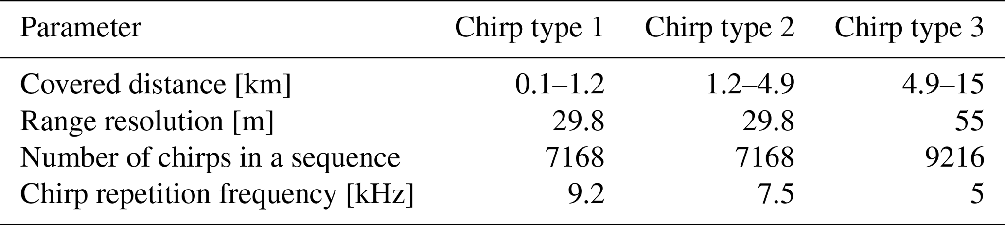
In order to check consistency of Eqs. (36), (39), (46), and (48) with radar measurements, I/Q data collected with a W-band cloud radar with the hybrid polarimetric mode were used (Myagkov and Unal, 2021). The radar is a part of a dual-frequency system owned and operated by the Technical University of Delft in Cabauw, the Netherlands. Technical specifications of the radar can be found in Myagkov et al. (2020). The radar uses frequency-modulated continuous signals. Küchler et al. (2017) explain the operation principle and show that the radar profiles the atmosphere using several chirp types. Each chirp type is dedicated to a certain distance range. During measurements chirp types are switched consequently. For each chirp type a number of chirps (chirp sequence hereafter) are processed continuously. Operational settings used during I/Q measurements are listed in Table 1.
Measurements were made during a rain event on 21 June 2021 at 7:44 UTC. I/Q measurements provide a high data rate of about 900 MB min−1. Therefore, about 3 min of I/Q measurements were collected for the analysis. The radar was pointed to 45∘ elevation. Since different chirp types have different properties, in the following only I/Q data collected with the first chirp type are used. Since the first chirp sequence covers the lowest part of the atmosphere, the analyzed data correspond to rain. As explained in Sect. 2, no noise subtraction is required to describe the statistics of the measurements. We therefore use all available spectral lines, including those containing noise only. A total of 90 % of spectral noise power was from 0.2–1.3 a.u (arbitrary units). Signal-to-noise ratio (defined here as a ratio of signal power in a spectral line divided by the mean spectral noise power in the same range bin) specified in linear units was from 0 (no signal) to 106. We would like to emphasize that no filtering based on signal-to-noise ratio was applied. Taking into account that the first chirp type has 37 range bins, in total 2.2×10³ chirp sequences (15.9×10⁶ chirps) are available in each polarimetric channel.
5.1 Processing
All I/Q measurements within a chirp sequence in every polarimetric channel are split into 224 continuous blocks. Each block contains 32 I/Q pairs. The FFT with the Blackman weighting window is applied to each block to get complex Doppler spectra. Then the 224 blocks are split into 28 sub-blocks with 8 spectra in each sub-block. Within each sub-block elements of the vector are calculated according to Eqs. (15)–(18) with Ns=8 for every spectral line. For each the vector is obtained. Note that for this, Eqs. (10)–(12) were applied to elements of instead of b. Using vectors and within a sequence, the error covariance matrices and are calculated numerically. The circumflex here indicates that the error covariance matrices are estimated from measurements.
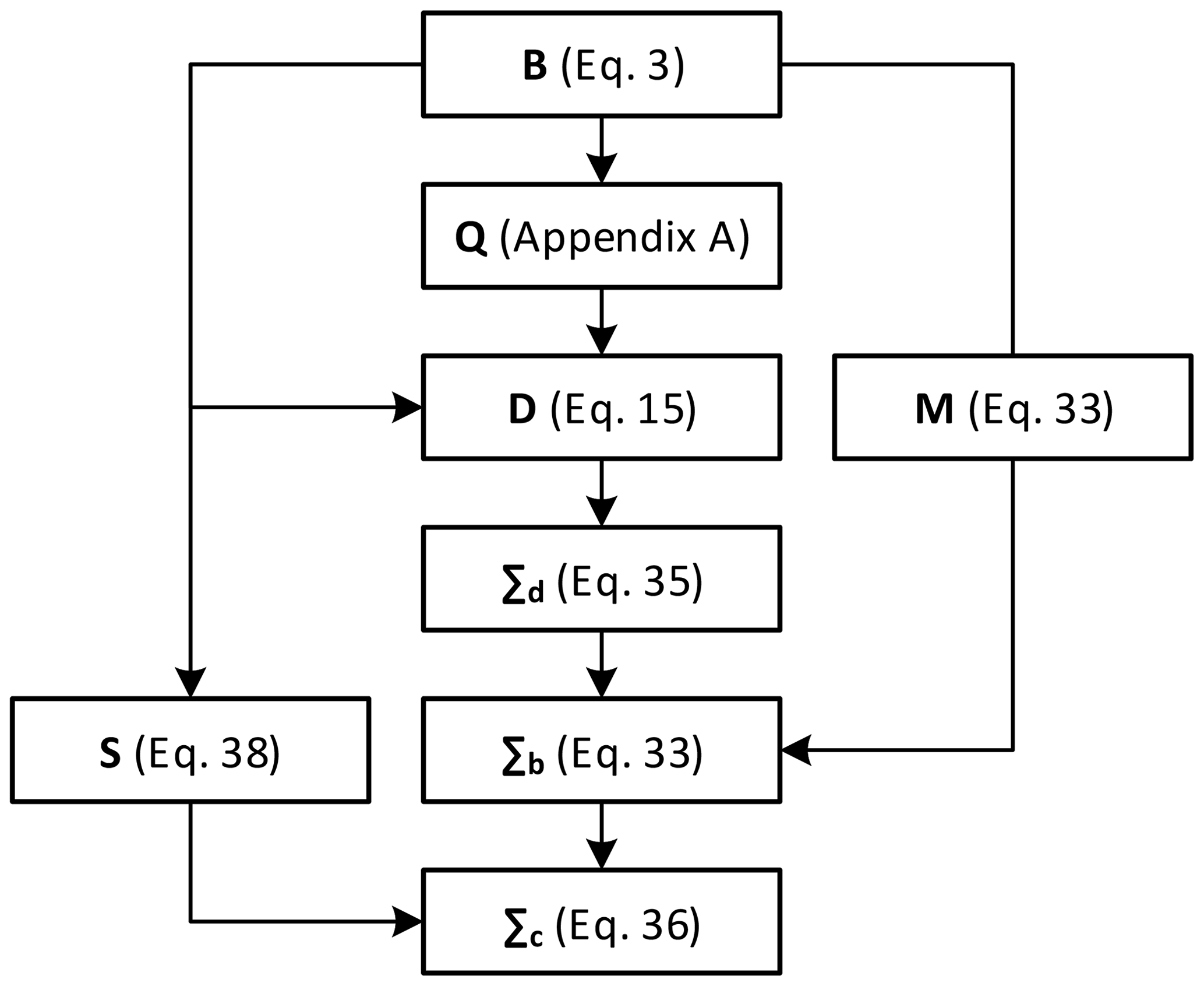
The calculation of the likelihood functions using Eqs. (36) and (39) requires b. The approximation of covariance matrices using Eqs. (46) and (48) requires the matrix B. In order to estimate b and B, elements of the vector are averaged over 28 sub-blocks available within a single chirp sequence. These averaged values are assumed to be elements of the vector b from which the matrix B is obtained. Using B and Ns=8, Σb and Σc are calculated for each chirp sequence as shown in Fig. 1.
5.2 Filtering
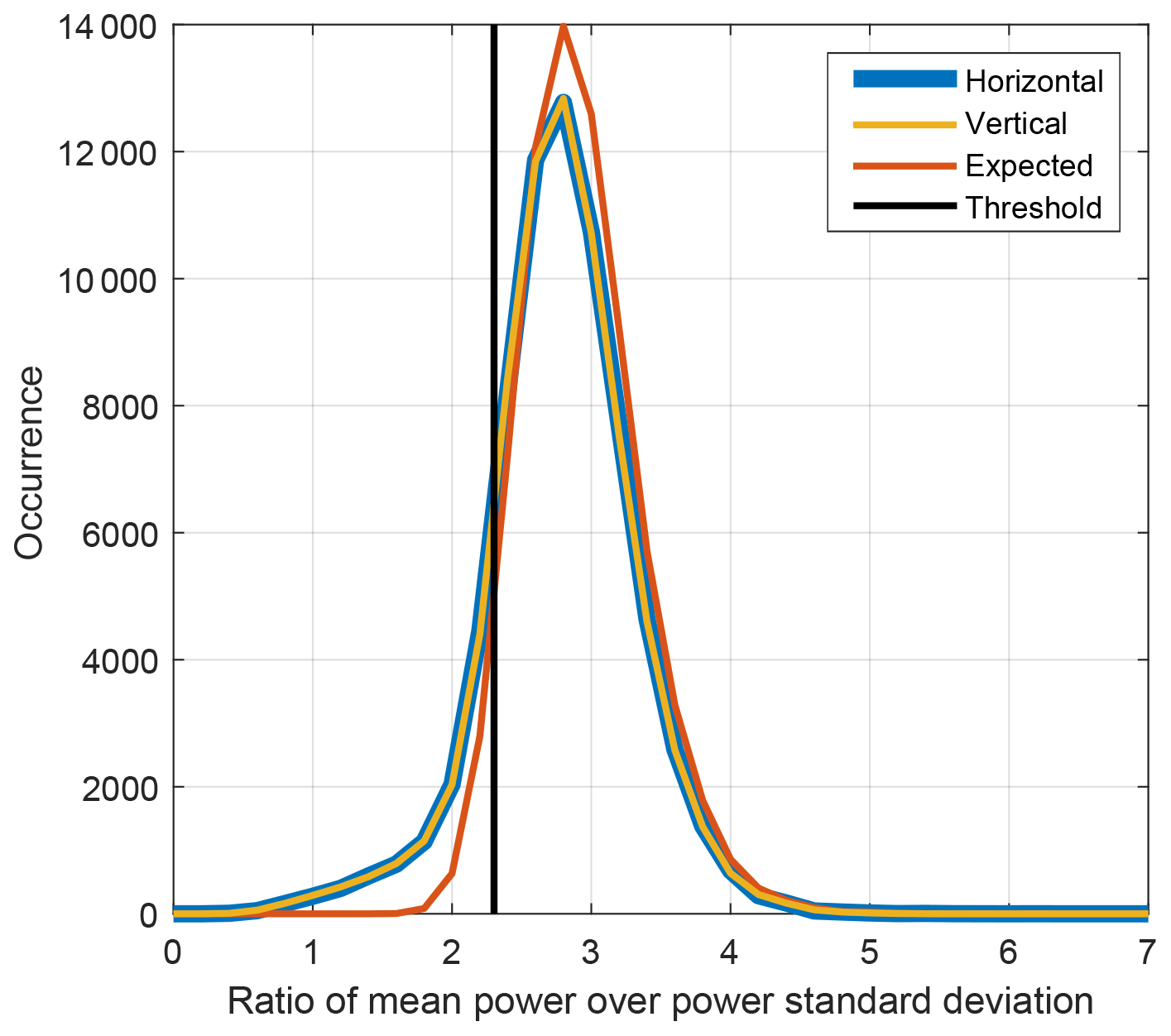
Figure 2Distributions of the ratio of mean power over the power standard deviation for the horizontal (blue line) and vertical (yellow line) channels. The expected distribution is shown with the red line. The vertical black line indicates the threshold corresponding to the 5th percentile of the distribution for the randomly generated complex numbers.
The random error analysis provided in this study is only applicable to volume-distributed scattering and noise. As discussed in Sect. 2, in this case is not correlated with , and is not correlated with . However, radar observations in general contain scattering from atmospheric plankton, ground clutter, and coherent receiver noise, which do not fulfill the assumption. In order to filter out spectral lines with correlated real and imaginary parts, a simple filtering rule was applied. It is known that for a signal with uncorrelated in-phase and quadrature components, its mean power and power standard deviation are related to each other (Eq. 5.193 in Bringi and Chandrasekar, 2001). Figure 2 shows distributions of the mean power over the power standard deviation calculated in the horizontal and vertical polarization channels shown by blue and yellow lines, respectively. It can be seen that the mode of the distributions is close to the theoretical value of . The distributions, however, have a considerable tail on the left side. These small values of the ratio are expected for correlated in-phase and quadrature components. Thus, a threshold in the ratio of the mean power over the standard deviation of power can be used to filter out unwanted spectral lines. In order to specify the threshold, the Monte Carlo approach was used. A total of 15.9×10⁶ random complex values with normal distribution, zero mean, and a standard deviation of 1 were generated. The same processing as for measured I/Q data was applied to the generated complex values. The distribution of the ratio of the mean power over the power standard deviation for the generated data (denoted as expected distribution) is shown in Fig. 2 by the red line. The expected distribution has a much smaller tail on the left side relative to the ones of the measured distributions. The threshold of 2.3 used for filtering is chosen as the 5th percentile of the expected distribution. Vectors and are excluded from the analysis if for the corresponding spectral component within a chirp sequence the ratio of the mean power over the power standard deviation is below the threshold in at least one of the polarimetric channels. Around 18 % of the data are excluded.
5.3 Evaluation of and
Recall that b is estimated from measurements by averaging all available sub-blocks within a chirp sequence; b, however, can also be estimated by maximization of the likelihood functions given in Eqs. (36) and (39). In this case, an optimization algorithm needs to be employed to find a set of elements of b corresponding to the global maximum in either Eq. (36) or Eq. (39). This study uses a derivative-free optimization method available by default in MATLAB (Lagarias et al., 1998). Since the optimization method minimizes a function, the likelihood functions were not used directly. Instead, the following cost functions were used for the minimization:
Here the index l runs over 28 sub-blocks within a chirp sequence. Equations (50) and (51) take into account that the consecutive vectors are not correlated. In this case the total likelihood of 28 vector 's is a product of likelihood of each individual . In order to avoid an overflow of double numbers, the logarithm was used. In this case the logarithm of the product is replaced by the sum of logarithms. The logarithm is a monotonically increasing function, and therefore it does not change the position of the maximum of the likelihood function. Finally, the minus sign was introduced to have a smaller value of a cost function corresponding to a higher value of the likelihood. For the evaluation, 1000 chirp sequences were chosen randomly for the maximum likelihood estimation using . In each chirp sequence a single spectral line was randomly chosen for the analysis. Thus, there are 28 vector 's available in each of the 1000 chirp sequences. For each sequence, the optimization algorithm requires an initial guess of b. In order to avoid local minima, five different initial guesses were used, which are a coefficient P multiplied by the first in the analyzed chirp sequence. The values of P were 0.5, 0.75, 1, 1.25, and 1.5. The solution giving the lowest cost function out of the five outcomes was chosen as the result. Similarly the maximum likelihood estimation using was done using independently chosen 1000 chirp sequences. Figure 3 shows a comparison of elements of b estimated by averaging over 28 sub-blocks and those estimated by the maximum likelihood approach. All panels show a good agreement indicated by the close-to-unity slope of the linear regression. Both (results in the first row of Fig. 3) and (results in the second row of Fig. 3) show the same level of agreement and, therefore, can be used with no difference.

Figure 3Comparison of elements of b estimated by averaging over 28 sub-blocks (x axis) with those estimated by the maximum likelihood approach (y axis); was used for (a)–(d). was used for (e)–(h). Each panel contains 1000 points described in the text. Linear regressions are shown by solid red lines. Each panel has a text box with the slope of the corresponding linear regression. Uncertainties in the slopes were estimated using bootstrapping. Note that units are not critical for the evaluation of the correctness of the derived likelihood functions. Therefore, arbitrary units (a.u.) are used.
5.4 Evaluation of Σc
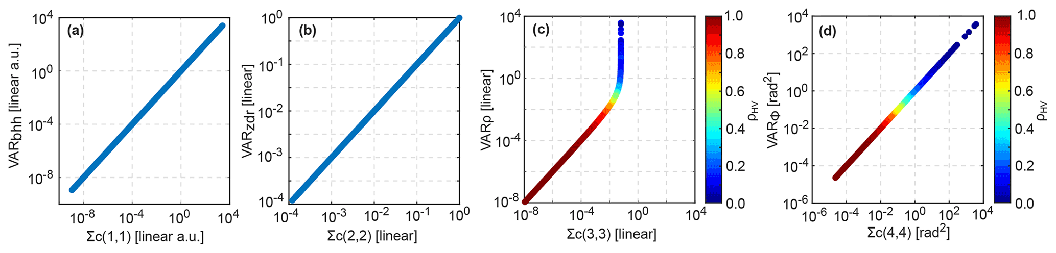
Figure 4Comparison of variances of (a) , (b) , (c) , and (d) . Approximations developed in this study are on the x axis. Approximations from Bringi and Chandrasekar (2001) are on the y axis; ρHV is color-coded in (c) and (d) to illustrate the values of ρHV at which approximations lead to erroneous values (see details in text). Note that units are not critical for the evaluation of the derived equations. Therefore, arbitrary units (a.u.) are used in (a).
Diagonal elements of Σc – variances of , , , and – were checked against those calculated using Eqs. (6.139a), (6.141), (6.144), and (6.143) in Bringi and Chandrasekar (2001), respectively. Taking into account that samples for a spectral line are not correlated, approximations for variances of , , , and based on the equations in Bringi and Chandrasekar (2001) are
respectively.
Figure 4 shows that VARbhh, VARzdr, and VARΦ match exactly Σc(1,1), Σc(2,2), and Σc(4,4), respectively. VARρ, however, agrees with Σc(3,3) only at values of ρHV>0.95. Below this value VARρ overestimates the variance of . At values of ρHV close to 0, VARρ has unrealistically high values, which result from ρHV in the denominator of Eq. (54).
Figure 4d also shows unrealistic values with both approximations of the variance. Taking into account that can take values within the range of 0 to 2π rad, the variance of exceeding 103 rad2 is definitely erroneous. The high variance of corresponds to values of ρHV<0.3. This effect results from the first-order Taylor approximation of Eq. (12), which is a highly non-linear function.

Figure 5Comparison of estimated from the radar measurements with Σc obtained from Eq. (48). Elements of Σc are given on the x axes. Elements of are given on the y axes. The first and the second numbers in brackets indicate the row and the column of the corresponding matrix, respectively. Linear regressions are shown by red lines. Slopes of the linear regressions and Pearson correlations are given in boxes in each panel. Uncertainties in the slope and the correlation are represented by ±1 standard deviation of the corresponding parameter. The standard deviations are obtained using bootstrapping. Panels without linear regressions show elements for which Eq. (48) gives only near-zero values. Note that units are not critical for the evaluation of the derived equations. Therefore, arbitrary units (a.u.) are used. Also note that only values on the x and y axes in an individual panel should be compared. Values in different panels should not be compared.
A comparison of the error covariance matrices with the calculated one Σc is shown in Fig. 5. Figure 5f, k, and p indicate considerable differences caused by the first-order Taylor approximation in variances of , , and , respectively. The results also reveal that the first-order Taylor approximation cannot adequately represent most of the non-diagonal components of the error covariance matrix.
5.5 Evaluation of Σb
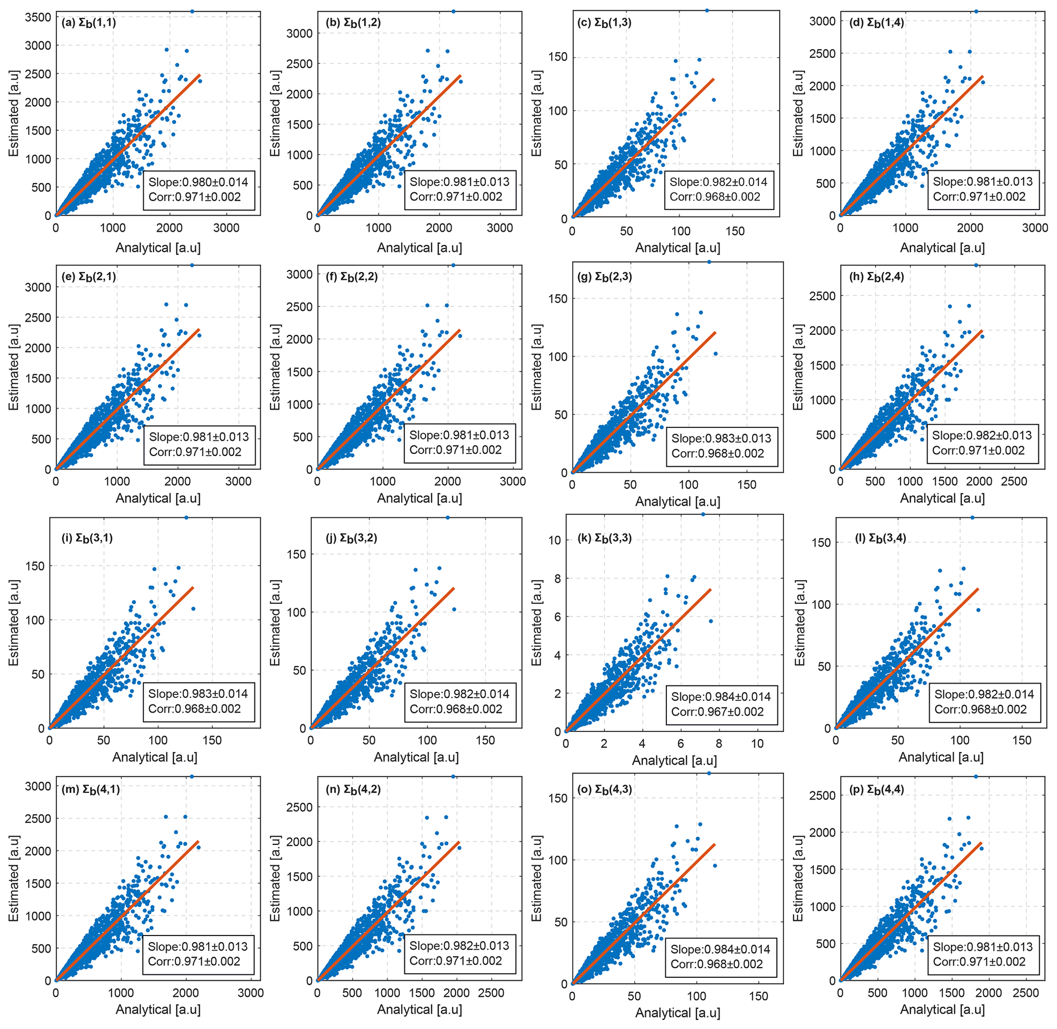
Figure 6Comparison of estimated from the radar measurements with Σb obtained from Eq. (46). Elements of Σb are given on the x axes. Elements of are given on the y axes. The first and the second numbers in brackets indicate the row and the column of the corresponding matrix, respectively. Linear regressions are shown by red lines. Slopes of the linear regressions and Pearson correlations are given in boxes in each panel. Uncertainties in the slope and the correlation are represented by ±1 standard deviation of the corresponding parameter. The standard deviations are obtained using bootstrapping. Note that units are not critical for the evaluation of the derived equations. Therefore, arbitrary units (a.u.) are used.
Figure 6 shows a comparison of elements of error covariance matrices estimated from the radar measurements with those calculated using Eq. (46). Estimated and calculated elements are in a good agreement. Linear regressions shown in the panels by red lines have slopes close to 1. Pearson correlations between estimated and calculated elements exceed 0.96. These results indicate an agreement of the theoretical calculation with measurements and thus confirm the correctness of Eq. (46). As expected, Figs. 6a and 5a show equivalent results. This is because the co-polar signal Bhh is effectively the same in both measurement representations and highlights the relevance of the present study only for dual-polarimetric quantities.
It is thus concluded that any application of spectral polarimetric measurements which requires the estimate of the error covariance matrix (e.g., variational retrievals, data assimilation, and sensitivity analysis) should be performed in the space of observations rather than .
Spectral and polarimetric cloud radar observations have a great potential in the cloud science (Kollias et al., 2020). Decades of such measurements have been already collected by, for example, the ARM (Atmospheric Radiation Measurement) and CLOUDNET communities. An advanced application of these vast datasets requires an accurate characterization of measurement uncertainties. Systematic errors in moment radar data and polarimetric variables have been discussed in many studies. Random measurement errors, in contrast, are rarely considered in the literature. There are three main problems in existing random-error-characterization methods in meteorological studies, namely (1) a lack of joint PDFs for averaged spectral polarimetric measurements, (2) neglection of non-diagonal components of the error covariance matrix, and (3) inaccuracy of the first-order approximation in variances of polarimetric variables. This study thus aims to provide solutions for these three problems.
Equations provided in Sect. 3 give an exact mathematical solution for the joint PDFs of spectral polarimetric observations. The PDFs are given for two equivalent representations of the measurements: (1) and (2) . The obtained equations take into account non-coherent averaging of spectra, which is applied by a majority of cloud radars to improve the sensitivity. Maximum likelihood estimators of b based on Eqs. (36) and (39) were compared with the estimator based on longer averaging. The comparison was based on dual-polarimetric cloud radar observations. The comparison showed a good agreement. Both PDFs can be equivalently used for methods based on the maximum likelihood and Bayesian inference.
Section 4 is focused on the error covariance matrix required for a number of applications such as data assimilation, sensitivity analysis, and variational retrievals. The error covariance matrices Σb and Σc for b and c, respectively, are obtained using the characteristic functions of the PDFs described in Sect. 3. Since the calculation of the c includes highly non-linear functions, Σc was derived using the first-order Taylor approximation. The same approach was used by Bringi and Chandrasekar (2001) to get equations for variances of polarimetric observations.
The error covariance matrices were evaluated using I/Q observations from a polarimetric W-band radar. It is illustrated that elements of Σc have considerable differences from those estimated from the measurements. First, we found differences in variances of ZDR, ρHV, and ΦDP of up to a factor of 10, 5, and 100, respectively. Second, the calculated variance of ΦDP shows unrealistically high values by far exceeding the range of possible values. Third, most of the off-diagonal terms of Σc are not correlated with corresponding values estimated from observations. We relate the differences to the first-order Taylor approximation. The Taylor approximation assumes linear relations between elements of the vector b and the elements of the vector c, while the relations include highly non-linear functions. In contrast, Σb agrees well with the observations. The correlation between calculated elements of Σb with those estimated from the observations exceeds 0.965.
Thus, based on the results found within this study, it is recommended to use the vector b to represent polarimetric cloud radar observations for applications requiring the error covariance matrix. This representation has a better characterization of random errors in comparison with widely used representation c. When the signal-to-noise ratio is high (>35 dB), however, the variances are quite low, and the Taylor approximation may give reasonable results. We would like to emphasize that there is no additional processing required to get the vector b. Elements of the vector b are an intermediate processing step on the way from I/Q data to conventional spectral polarimetric variables and thus have been already calculated by Doppler cloud radars with the hybrid mode.
In order to demonstrate a practical application of the developed characterization of the measurements errors, a few retrieval techniques are currently being developed. The first one is an improvement of the ice-shape retrieval described in Myagkov et al. (2016a). Another one is an adoption of the drop size distribution retrieval from Tridon and Battaglia (2015) for dual-polarimetric cloud radar observations.
The operator Q, which is used to diagonalize the covariance matrix B in Eq. (20), is calculated as follows (Kanareykin et al., 1968, chap. 2.5):
where
In Eq. (A4) Tr is the matrix trace.
B1 Change in variables in a PDF
Consider a vector a with n random variables a1…n. Assume the joint PDF fa(a) of the variables is known. The joint PDF fy(y) of a vector
can be found by changing the variables in fa(a):
where G−1 is the reverse transformation from y to a, and J is the determinant of the Jacobian of the transformation .
B2 Likelihood functions for Dcc and Dxx
It is known that the PDF of zs being a sum of squares of independent standard normal samples (i.e., distributed normally with a mean of 0 and standard deviation of 1) is the chi-squared distribution , where the degree of freedom k shows how many samples have been summed. Taking into account that
where the first and the second summed terms in the curly brackets are sums of squares of independent standard normal samples, the likelihood function can be found by changing the variable zs to :
The factor of 2 in the degree of freedom is because there are 2Ns summed components in the curly brackets in Eq. (B3). The equation for is derived in a similar manner as for , resulting in
B3 Likelihood functions for Rcx and Jcx
Nadarajah and Pogány (2016) provide a solution for the PDF of an averaged multiplication zm of two standard normal variables. For two uncorrelated variables the PDF is defined as follows:
where n is the number of averaged multiplications, Γ is the gamma function, and Kμ is the Bessel function of the second kind of order μ.
is calculated as follows:
where the term in the curly brackets is an average over 2Ns multiplications of independent standard normal samples. In this case, the likelihood function can be found by changing zm by :
where , , Γ is the gamma function, and Kμ is the Bessel function of the second kind of order μ. When , the modified Bessel function . Therefore, for close to 0, the following approximation based on Eqs. (9.6.6) and (9.6.8) from Abramowitz and Stegun (1972) should be used:
Formulas for are defined in a similar manner:
The approximation for is close to 0:
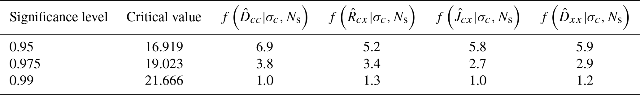
B4 Monte Carlo evaluation of Eqs. (B4), (B5), (B8), and (B10)
Table B1Percentage of test-statistic values exceeding critical values for different significance levels. Percentages are given in percent. The names of the four columns on the right side of the table indicate the distribution for which a percentage is given.
For the equation evaluation a simulated dataset was generated. In total 1000 sets of distributions were simulated using the Monte Carlo approach. A single set included distributions of , , , and . For a single set 105 vector 's were generated. A single vector resulted from Ns randomly generated vector m's. For a single set of distributions a single covariance matrix B was taken. The elements of the covariance matrix B and Ns were randomly generated according to the following rules (values have linear arbitrary units):
-
Bhh is a sum of mean powers of signal Psh and noise Pnh.
-
Bvv is a sum of mean powers of signal Psv and noise Pnv.
-
.
-
Psh and Psv were randomly and independently generated using the uniform distribution from 1 to 5.
-
was calculated as .
-
ρHV was chosen randomly using the uniform distribution from 0 to 1.
-
ΦDP was chosen randomly using the uniform distribution from 0 to 2π.
-
Ns was chosen as a random integer number in the range of 2 to 80.
From the covariance matrix B the true covariance matrix Σm was obtained. A total of 105×Ns vector m's were generated according to the PDF given in Eq. (2). Then, 105 elements of the were calculated according to Eqs. (15)–(18). Elements of the vector were derived from the vector 's using Eq. (27).
Using the 105 vector 's individual histograms for each of the variables , , , and are derived. A histogram has 10 bins covering the range from the minimum to maximum values of the corresponding variable. Widths of bins were adjusted to have 10 000 samples in each bin. For the same bins the expected number of samples is calculated using the corresponding PDF. Since integration of Eqs. (B4), (B5), (B8), and (B10) is challenging, the integration is done numerically. Then the Pearson's chi-squared test is applied. The same procedure is repeated for all 1000 sets of distributions. Thus, for each PDF (Eqs. B4, B5, B8, and B10) 1000 test-statistic values were obtained.
The Pearson's chi-squared test implies a comparison of the test-statistic values with critical values for a given level of significance. A test-statistic value exceeding the critical value would indicate that there is a chance (equal to the significance level) that the data significantly differ from the PDF. There is, however, a small chance that the conclusion that the data differ from the PDF is erroneous. Table B1 shows the percentage of the test-statistic values exceeding critical values. It can be seen that the number of test-statistic values exceeding corresponding critical values is very close to the theoretical values, i.e., 5, 2.5, and 1 % at 0.95, 0.975, and 0.99 significance levels, respectively. This confirms the validity of the obtained PDFs.
To derive solutions for the mean and variances of elements of , the distribution of the elements is represented by characteristic functions. A γth raw statistical moment Mγ of a random variable with a characteristic function ϕ(t) can be found as follows:
The calculation of derivatives of the characteristic functions is in general easier to obtain than integration of the corresponding PDFs.
The characteristic function of the chi-squared distribution is
Therefore, the characteristic function for for a given σc and Ns can be written in the following way:
The mean value and variance of are calculated as follows:
Similarly,
Based on Nadarajah and Pogány (2016) the characteristic function corresponding to fz(zm) is
Therefore, the characteristic function for and for given σc, σx, and Ns is as follows:
As expected for a multiplication of two uncorrelated variables, the mean values of and are as follows:
The variance of and can be found as follows:
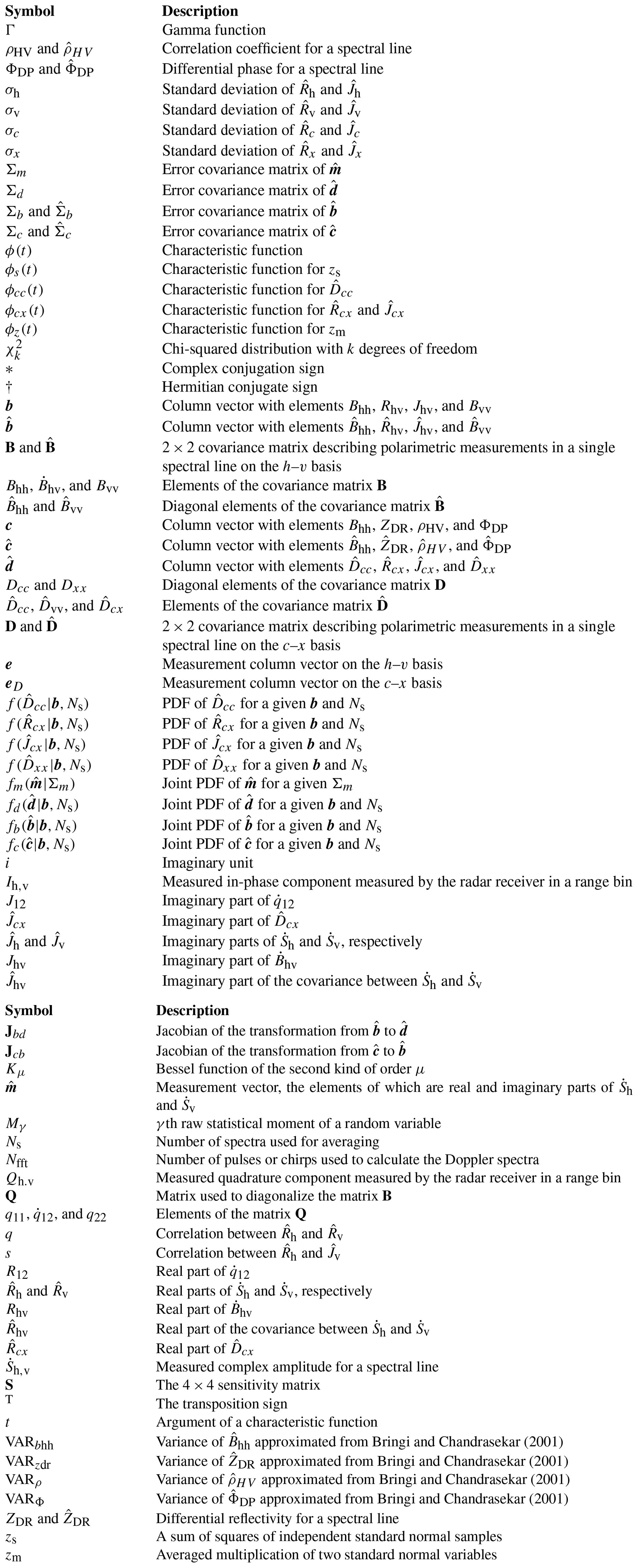
Table G1Main symbols used throughout the study. The overdot indicates a complex number. Indices h and v indicate the polarization of the receiver channel. The circumflex indicates a measured quantity.
I/Q data used in this study are available on Zenodo (Myagkov and Unal, 2021). MATLAB code used to process I/Q data is provided in the Supplement to this paper. Ready-to-use MATLAB implementations for Eqs. (36), (39), (46), and (48) are given in the Supplement.
The supplement related to this article is available online at: https://doi.org/10.5194/amt-15-1333-2022-supplement.
AM derived equations for PDFs and error covariance matrices, made evaluation using the radar observations, and prepared the first draft of the manuscript. DO reviewed the draft and essentially improved the manuscript.
Alexander Myagkov is an employee of Radiometer Physics GmbH, and Davide Ori has no competing interests.
Publisher’s note: Copernicus Publications remains neutral with regard to jurisdictional claims in published maps and institutional affiliations.
This article is part of the special issue “Fusion of radar polarimetry and numerical atmospheric modelling towards an improved understanding of cloud and precipitation processes (ACP/AMT/GMD inter-journal SI)”. It is not associated with a conference.
This work was carried out as a collaboration within the IMPRINT (Understanding Ice Microphysical Processes by combining multi-frequency and spectral Radar polarImetry aNd super-parTicle modelling) project (project no. 408011764), which is a part of the German Research Foundation (DFG) Priority Program SPP2115 PROM (Fusion of Radar Polarimetry and Numerical Atmospheric Modelling Towards an Improved Understanding of Cloud and Precipitation Processes). The authors acknowledge Ruisdael Observatory (the Netherlands) and Christine Unal from TU Delft for granting access to the W-band radar in Cabauw to collect I/Q data used in this study. The work of Davide Ori is funded by the German Research Foundation (DFG) under the grant SCHE 2074/1-1 (SPP HALO). The authors thank the editor and the two reviewers for comments and suggestions, which helped to improve the paper.
Radiometer Physics GmbH covered the publication fees.
This paper was edited by Ulrich Löhnert and reviewed by Dmitri Moisseev and one anonymous referee.
Abramowitz, M. and Stegun, I. A.: Handbook of Mathematical Functions With Formulas, Graphs, and Mathematical Tables, in: Applied Mathematics Series 55, 10th edn., edited by: Abramowitz, M. and Stegun, I. A., United States National Bureau of Standards, 1972.
Acquistapace, C., Kneifel, S., Löhnert, U., Kollias, P., Maahn, M., and Bauer-Pfundstein, M.: Optimizing observations of drizzle onset with millimeter-wavelength radars, Atmos. Meas. Tech., 10, 1783–1802, https://doi.org/10.5194/amt-10-1783-2017, 2017.
Borque, P., Luke, E., and Kollias, P.: On the unified estimation of turbulence eddy dissipation rate using Doppler cloud radars and lidars, J. Geophys. Res.-Atmos., 121, 5972–5989, https://doi.org/10.1002/2015JD024543, 2016.
Bringi, V. N. and Chandrasekar, V.: Polarimetric Doppler Weather Radar, Cambridge University Press, ISBN 0521623847, 2001.
Bühl, J., Ansmann, A., Seifert, P., Baars, H., and Engelmann, R.: Toward a quantitative characterization of heterogeneous ice formation with lidar/radar: Comparison of CALIPSO/CloudSat with ground-based observations, Geophys. Res. Lett., 40, 4404–4408, https://doi.org/10.1002/grl.50792, 2013.
Bühl, J., Seifert, P., Engelmann, R., and Ansmann, A.: Impact of vertical air motions on ice formation rate in mixed-phase cloud layers, NPJ Clim. Atmos. Sci., 2, 36, https://doi.org/10.1038/s41612-019-0092-6, 2019a.
Bühl, J., Seifert, P., Radenz, M., Baars, H., and Ansmann, A.: Ice crystal number concentration from lidar, cloud radar and radar wind profiler measurements, Atmos. Meas. Tech., 12, 6601–6617, https://doi.org/10.5194/amt-12-6601-2019, 2019b.
Cao, Q., Zhang, G., and Xue, M.: A Variational Approach for Retrieving Raindrop Size Distribution from Polarimetric Radar Measurements in the Presence of Attenuation, J. Appl. Meteorol. Clim., 52, 169–185, https://doi.org/10.1175/JAMC-D-12-0101.1, 2013.
Chandrasekar, V., Baldini, L., Bharadwaj, N., and Smith, P. L.: Calibration procedures for global precipitation-measurement ground-validation radars, URSI Radio Sci. Bull., 2015, 45–73, https://ieeexplore.ieee.org/document/7909473 (last access: 6 March 2022), 2015.
Chang, W.-Y., Vivekanandan, J., Ikeda, K., and Lin, P.-L.: Quantitative Precipitation Estimation of the Epic 2013 Colorado Flood Event: Polarization Radar-Based Variational Scheme, J. Appl. Meteorol. Clim., 55, 1477–1495, https://doi.org/10.1175/JAMC-D-15-0222.1, 2016.
Doviak, R. J., Zrnic, D. S., and Sirmans, D. S.: Doppler weather radar, Proc. IEEE, 67, 1522–1553, https://doi.org/10.1109/PROC.1979.11511, 1979.
Dufournet, Y. and Russchenberg, H. W. J.: Towards the improvement of cloud microphysical retrievals using simultaneous Doppler and polarimetric radar measurements, Atmos. Meas. Tech., 4, 2163–2178, https://doi.org/10.5194/amt-4-2163-2011, 2011.
Görsdorf, U., Lehmann, V., Bauer-Pfundstein, M., Peters, G., Vavriv, D., Vinogradov, V., and Volkov, V.: A 35-GHz polarimetric Doppler radar for long term observations of cloud parameters – Description of system and data processing, J. Atmos. Ocean. Tech., 32, 675–690, https://doi.org/10.1175/JTECH-D-14-00066.1, 2015.
Hildebrand, P. H. and Sekhon, R. S.: Objective determination of the noise level in Doppler spectra, J. Appl. Meteorol., 13, 808–811, https://doi.org/10.1175/1520-0450(1974)013<0808:ODOTNL>2.0.CO;2, 1974.
Hogan, R. J.: A Variational Scheme for Retrieving Rainfall Rate and Hail Reflectivity Fraction from Polarization Radar, J. Appl. Meteorol. Clim., 46, 1544, https://doi.org/10.1175/JAM2550.1, 2007.
Huang, H., Zhao, K., Zhang, G., Hu, D., and Yang, Z.: Optimized raindrop size distribution retrieval and quantitative rainfall estimation from polarimetric radar, J. Hydrol., 580, 124248, https://doi.org/10.1016/j.jhydrol.2019.124248, 2020.
Illingworth, A. J., Hogan, R. J., O'Connor, E. J., Bouniol, D., Delanoé, J., Pelon, J., Protat, A., Brooks, M. E., Gaussiat, N., Wilson, D. R., Donovan, D. P., Baltink, H. K., van Zadelhoff, G.-J., Eastment, J. D., Goddard, J. W. F., Wrench, C. L., Haeffelin, M., Krasnov, O. A., Russchenberg, H. W. J., Piriou, J.-M., Vinit, F., Seifert, A., Tompkins, A. M., and Willén, U.: Cloudnet, B. Am. Meteorol. Soc., 88, 883–898, https://doi.org/10.1175/BAMS-88-6-883, 2007.
Kalesse, H., Szyrmer, W., Kneifel, S., Kollias, P., and Luke, E.: Fingerprints of a riming event on cloud radar Doppler spectra: observations and modeling, Atmos. Chem. Phys., 16, 2997–3012, https://doi.org/10.5194/acp-16-2997-2016, 2016.
Kanareykin, D. B., Potechin, V. A., and Shishkin, I. F.: Marine Radio Polarimetry, Sudostroenie, 1968.
Kneifel, S. and Moisseev, D.: Long-Term Statistics of Riming in Nonconvective Clouds Derived from Ground-Based Doppler Cloud Radar Observations, J. Atmos. Sci., 77, 3495–3508, https://doi.org/10.1175/JAS-D-20-0007.1, 2020.
Kneifel, S., von Lerber, A., Tiira, J., Moisseev, D., Kollias, P., and Leinonen, J.: Observed relations between snowfall microphysics and triple-frequency radar measurements, J. Geophys. Res.-Atmos., 6034–6055, 2015JD023156, https://doi.org/10.1002/2015JD023156, 2015.
Kneifel, S., Kollias, P., Battaglia, A., Leinonen, J., Maahn, M., Kalesse, H., and Tridon, F.: First observations of triple-frequency radar Doppler spectra in snowfall: Interpretation and applications, J. Geophys. Res.-Atmos., 43, 2225–2233, https://doi.org/10.1002/2015GL067618, 2016.
Kollias, P., Clothiaux, E. E., Miller, M. A., Albrecht, B. A., Stephens, G. L., and Ackerman, T. P.: Millimeter-Wavelength Radars: New Frontier in Atmospheric Cloud and Precipitation Research, B. Am. Meteorol. Soc., 88, 1608–1624, https://doi.org/10.1175/BAMS-88-10-1608, 2007.
Kollias, P., Bharadwaj, N., Clothiaux, E. E., Lamer, K., Oue, M., Hardin, J., Isom, B., Lindenmaier, I., Matthews, A., Luke, E. P., Giangrande, S. E., Johnson, K., Collis, S., Comstock, J., and Mather, J. H.: The ARM Radar Network: At the Leading Edge of Cloud and Precipitation Observations, B. Am. Meteorol. Soc., 101, E588–E607, https://doi.org/10.1175/BAMS-D-18-0288.1, 2020.
Küchler, N., Kneifel, S., Löhnert, U., Kollias, P., Czekala, H., and Rose, T.: A W-Band Radar-Radiometer System for Accurate and Continuous Monitoring of Clouds and Precipitation, J. Atmos. Ocean. Tech., 34, 2375–2392, https://doi.org/10.1175/JTECH-D-17-0019.1, 2017.
Kumjian, M.: Principles and Applications of Dual-Polarization Weather Radar. Part I: Description of the Polarimetric Radar Variables, J. Operational Meteor., 1, 226–242, https://doi.org/10.15191/nwajom.2013.0119, 2013.
Lagarias, J. C., Reeds, J. A., Wright, M. H., and Wright, P. E.: Convergence Properties of the Nelder–Mead Simplex Method in Low Dimensions, SIAM J. Optim., 9, 112–147, https://doi.org/10.1137/S1052623496303470, 1998.
Lee, J.-S., Hoppel, K. W., Mango, S. A., and Miller, A. R.: Intensity and phase statistics of multilook polarimetric and interferometric SAR imagery, IEEE T. Geosci. Remote, 32, 1017–1028, https://doi.org/10.1109/36.312890, 1994.
Lu, Y., Aydin, K., Clothiaux, E. E., and Verlinde, J.: Retrieving Cloud Ice Water Content Using Millimeter- and Centimeter-Wavelength Radar Polarimetric Observables, J. Appl. Meteorol. Clim., 54, 596–604, https://doi.org/10.1175/JAMC-D-14-0169.1, 2015.
Marple, S.: Digital Spectral Analysis, 2nd edn., Dover Books on Electrical Engineering, Dover Publications, ISBN 9780486780528, 2019.
Matrosov, S. Y.: Attenuation-Based Estimates of Rainfall Rates Aloft with Vertically Pointing Ka-Band Radars, J. Atmos. Ocean. Tech., 22, 43, https://doi.org/10.1175/JTECH-1677.1, 2005.
Matrosov, S. Y., Reinking, R. F., Kropfli, R. A., Martner, B. E., and Bartram, B. W.: On the Use of Radar Depolarization Ratios for Estimating Shapes of Ice Hydrometeors in Winter Clouds, J. Appl. Meteorol., 40, 479–490, https://doi.org/10.1175/1520-0450(2001)040<0479:OTUORD>2.0.CO;2, 2001.
Matrosov, S. Y., May, P. T., and Shupe, M. D.: Rainfall Profiling Using Atmospheric Radiation Measurement Program Vertically Pointing 8-mm Wavelength Radars, J. Atmos. Ocean. Tech., 23, 1478, https://doi.org/10.1175/JTECH1957.1, 2006.
Matrosov, S. Y., Shupe, M. D., and Djalalova, I. V.: Snowfall Retrievals Using Millimeter-Wavelength Cloud Radars, J. Appl. Meteorol. Clim., 47, 769, https://doi.org/10.1175/2007JAMC1768.1, 2008.
Matrosov, S. Y., Mace, G. G., Marchand, R., Shupe, M. D., Hallar, A. G., and McCubbin, I. B.: Observations of ice crystal habits with a scanning polarimetric W-band radar at slant linear depolarization ratio mode, J. Atmos. Ocean. Tech., 29, 989–1008, https://doi.org/10.1175/JTECH-D-11-00131.1, 2012.
Matrosov, S. Y., Schmitt, C. G., Maahn, M., and de Boer, G.: Atmospheric Ice Particle Shape Estimates from Polarimetric Radar Measurements and In Situ Observations, J. Atmos. Ocean. Tech., 34, 2569–2587, https://doi.org/10.1175/JTECH-D-17-0111.1, 2017.
Middleton, D.: An Introduction to Statistical Communication Theory: An IEEE Press Classic Reissue, Wiley, ISBN 9780780311787, 1996.
Moisseev, D. N. and Chandrasekar, V.: Nonparametric Estimation of Raindrop Size Distributions from Dual-Polarization Radar Spectral Observations, J. Atmos. Ocean. Tech., 24, 1008, https://doi.org/10.1175/JTECH2024.1, 2007.
Moisseev, D., von Lerber, A., and Tiira, J.: Quantifying the effect of riming on snowfall using ground-based observations, J. Geophys. Res.-Atmos., 122, 4019–4037, https://doi.org/10.1002/2016JD026272, 2017.
Morrison, H., van Lier-Walqui, M., Fridlind, A. M., Grabowski, W. W., Harrington, J. Y., Hoose, C., Korolev, A., Kumjian, M. R., Milbrandt, J. A., Pawlowska, H., Posselt, D. J., Prat, O. P., Reimel, K. J., Shima, S.-I., van Diedenhoven, B., and Xue, L.: Confronting the Challenge of Modeling Cloud and Precipitation Microphysics, J. Adv. Model. Earth Sy., 12, e01689, https://doi.org/10.1029/2019MS001689, 2020.
Myagkov, A. and Unal, C.: W-band dataset with I/Q measurement for an AMT manuscript (1.0), Zenodo [data set], https://doi.org/10.5281/zenodo.5126813, 2021.
Myagkov, A., Seifert, P., Wandinger, U., Bauer-Pfundstein, M., and Matrosov, S. Y.: Effects of antenna patterns on cloud radar polarimetric measurements, J. Atmos. Ocean. Tech., 32, 1813–1828, https://doi.org/10.1175/JTECH-D-15-0045.1, 2015.
Myagkov, A., Seifert, P., Bauer-Pfundstein, M., and Wandinger, U.: Cloud radar with hybrid mode towards estimation of shape and orientation of ice crystals, Atmos. Meas. Tech., 9, 469–489, https://doi.org/10.5194/amt-9-469-2016, 2016a.
Myagkov, A., Seifert, P., Wandinger, U., Bühl, J., and Engelmann, R.: Relationship between temperature and apparent shape of pristine ice crystals derived from polarimetric cloud radar observations during the ACCEPT campaign, Atmos. Meas. Tech., 9, 3739–3754, https://doi.org/10.5194/amt-9-3739-2016, 2016b.
Myagkov, A., Kneifel, S., and Rose, T.: Evaluation of the reflectivity calibration of W-band radars based on observations in rain, Atmos. Meas. Tech., 13, 5799–5825, https://doi.org/10.5194/amt-13-5799-2020, 2020.
Nadarajah, S. and Pogány, T. K.: On the distribution of the product of correlated normal random variables, C. R. Math., 354, 201–204, https://doi.org/10.1016/j.crma.2015.10.019, 2016.
Oue, M., Kumjian, M. R., Lu, Y., Verlinde, J., Aydin, K., and Clothiaux, E. E.: Linear depolarization ratios of columnar ice crystals in a deep precipitating system over the Arctic observed by zenith-pointing Ka-band Doppler radar, J. Appl. Meteorol. Clim., 54, 1060–1068, https://doi.org/10.1175/JAMC-D-15-0012.1, 2015.
Oue, M., Kollias, P., Ryzhkov, A., and Luke, E. P.: Toward Exploring the Synergy Between Cloud Radar Polarimetry and Doppler Spectral Analysis in Deep Cold Precipitating Systems in the Arctic, J. Geophys. Res.-Atmos., 123, 2797–2815, https://doi.org/10.1002/2017JD027717, 2018.
Pfitzenmaier, L., Unal, C. M. H., Dufournet, Y., and Russchenberg, H. W. J.: Observing ice particle growth along fall streaks in mixed-phase clouds using spectral polarimetric radar data, Atmos. Chem. Phys., 18, 7843–7862, https://doi.org/10.5194/acp-18-7843-2018, 2018.
Rodgers, C. D.: Inverse Methods for Atmospheric Sounding, Series on Atmospheric, Oceanic and Planetary Physics, 2, ISBN 981022740X, World Scientific, https://doi.org/10.1142/3171, 2000.
Rusli, S. P., Donovan, D. P., and Russchenberg, H. W. J.: Simultaneous and synergistic profiling of cloud and drizzle properties using ground-based observations, Atmos. Meas. Tech., 10, 4777–4803, https://doi.org/10.5194/amt-10-4777-2017, 2017.
Ryzhkov, A. V., Snyder, J., Carlin, J. T., Khain, A., and Pinsky, M.: What Polarimetric Weather Radars Offer to Cloud Modelers: Forward Radar Operators and Microphysical/Thermodynamic Retrievals, Atmosphere, 11, 362, https://doi.org/10.3390/atmos11040362, 2020.
Skolnik, M.: Radar Handbook, 3rd edn., McGraw-Hill Education, ISBN 9780071485470, 2008.
Spek, A. L. J., Unal, C. M. H., Moisseev, D. N., Russchenberg, H. W. J., Chandrasekar, V., and Dufournet, Y.: A new technique to categorize and retrieve the microphysical properties of ice particles above the melting layer using radar dual-polarization spectral analysis, J. Atmos. Ocean. Tech., 25, 482–497, https://doi.org/10.1175/2007JTECHA944.1, 2008.
Tridon, F. and Battaglia, A.: Dual-frequency radar Doppler spectral retrieval of rain drop size distributions and entangled dynamics variables, J. Geophys. Res.-Atmos., 120, 5585–5601, https://doi.org/10.1002/2014JD023023, 2015.
Tridon, F., Battaglia, A., Luke, E., and Kollias, P.: Rain retrieval from dual-frequency radar Doppler spectra: validation and potential for a midlatitude precipitating case-study, Q. J. Roy. Meteor. Soc., 143, 1364–1380, https://doi.org/10.1002/qj.3010, 2017.
Tridon, F., Battaglia, A., Chase, R. J., Turk, F. J., Leinonen, J., Kneifel, S., Mroz, K., Finlon, J., Bansemer, A., Tanelli, S., Heymsfield, A. J., and Nesbitt, S. W.: The Microphysics of Stratiform Precipitation During OLYMPEX: Compatibility Between Triple-Frequency Radar and Airborne In Situ Observations, J. Geophys. Res.-Atmos., 124, 8764–8792, https://doi.org/10.1029/2018JD029858, 2019.
Walpole, R. E., Myers, R. H., Myers, S. L., and Ye, K.: Probability and Statistics for Engineers and Scientists, 9th edn., edited by: Lynch, D., Prentice Hall, ISBN 9780321629111, 2012.
Wiener, N.: Generalized harmonic analysis, Acta Math., 55, 117–258, 1930.
Wilks, D. S.: Statistical methods in the atmospheric sciences, 3rd edn., in: International geophysics series, 100, ISBN 9780123850225, 2011.
Yoshikawa, E., Chandrasekar, V., and Ushio, T.: Raindrop Size Distribution (DSD) Retrieval for X-Band Dual-Polarization Radar, J. Atmos. Ocean. Tech., 31, 387–403, https://doi.org/10.1175/JTECH-D-12-00248.1, 2014.
Zhang, G., Mahale, V. N., Putnam, B. J., Qi, Y., Cao, Q., Byrd, A. D., Bukovcic, P., Zrnic, D. S., Gao, J., Xue, M., Jung, Y., Reeves, H. D., Heinselman, P. L., Ryzhkov, A., Palmer, R. D., Zhang, P., Weber, M., Mcfarquhar, G. M., Moore, B., Zhang, Y., Zhang, J., Vivekanandan, J., Al-Rashid, Y., Ice, R. L., Berkowitz, D. S., Tong, C.-c., Fulton, C., and Doviak, R. J.: Current Status and Future Challenges of Weather Radar Polarimetry: Bridging the Gap between Radar Meteorology/Hydrology/Engineering and Numerical Weather Prediction, Adv. Atmos. Sci., 36, 571–588, https://doi.org/10.1007/s00376-019-8172-4, 2019.
- Abstract
- Introduction
- Basics of radar spectral polarimetry in the hybrid mode
- Likelihood of elements of the covariance matrix B
- Error covariance matrices
- Consistency checks on radar observations
- Summary and outlook
- Appendix A: Diagonalization matrix Q
- Appendix B: Derivation of likelihood functions
- Appendix C: Variances of elements of the vector
- Appendix D: Sensitivity S
- Appendix E: Jacobian Jbd of the transformation from to
- Appendix F: Jacobian Jcb of the transformation from to
- Appendix G: Table of symbols
- Code and data availability
- Author contributions
- Competing interests
- Disclaimer
- Special issue statement
- Acknowledgements
- Financial support
- Review statement
- References
- Supplement