Characteristics of the derived energy dissipation rate using the 1 Hz commercial aircraft quick access recorder (QAR) data

The cube root of the energy dissipation rate (EDR), as a standard reporting metric of atmospheric turbulence, is estimated using 1 Hz quick access recorder (QAR) data from Korean-based national air carriers with two different types of aircraft (Boeing 737 (B737) and Boeing 777 (B777)), archived for 12 months from January to December 2012. The EDRs are estimated using three wind components (zonal, meridional, and derived vertical wind) and the derived equivalent vertical gust (DEVG) of the 1 Hz post-flight data by applying all possible EDR methods. Wind components are used to calculate three different EDRs, utilizing the second-order structure function, power spectral density, and von Kármán wind spectrum and maximum-likelihood method. In addition, two DEVG-based EDRs are calculated using the lognormal mapping technique and the predefined parabolic relationship between the observed EDR and DEVG. When the reliability of lower-rate (1 Hz) data to estimate the EDR is examined using the higher-rate (20 Hz) wind data obtained from a tall tower observatory, it is found that the 1 Hz EDR can be underestimated (2.19 %–12.56 %) or overestimated (9.32 %–10.91 %). In this study, it is also found that the structure-function-based EDR shows lower uncertainty (2.19 %–8.14 %) than the energy spectrum-based EDRs (9.32 %–12.56 %) when the 1 Hz datasets are used. The observed EDR estimates using 1 Hz QAR data are examined in three strong turbulence cases that are relevant to clear-air turbulence (CAT), mountain wave turbulence (MWT), and convectively induced turbulence (CIT). The observed EDR estimates derived from three different wind components show different characteristics depending on potential sources of atmospheric turbulence at cruising altitudes, indicating good agreement with selected strong turbulence cases with respect to turbulence intensity and incident time. Zonal wind-based EDRs are stronger in the CAT case that is affected by synoptic-scale forcing such as upper-level jet/frontal system. In the CIT case, vertical wind-based EDRs are stronger, which is related to convectively induced gravity waves outside the cloud boundary. The MWT case has a peak of the EDR based on both the zonal and vertical winds, which can be related to the propagation of mountain waves and their subsequent breaking. It is also found that the CAT and MWT cases occurred by synoptic-scale forcing have longer variations in the observed EDRs before and after the turbulence incident, while the CIT case triggered by a mesoscale convective cell has an isolated peak of the EDR. Current results suggest that the 1 Hz aircraft data can be an additional source of the EDR estimations contributing to expand more EDR information at the cruising altitudes in the world and that these data can be helpful to provide a better climatology of aviation turbulence and a situational awareness of cruising aircraft.

1 Introduction

Turbulence encounters are major threats to the aviation industry that can result in serious structural damage to aircraft and injuries to passengers and flight crew (Sharman and Lane, 2016; Gultepe et al., 2019). To mitigate the risk associated with turbulence, the use of a large number of reliable turbulence observations is essential, both for extending our understanding of turbulence and accurately forecasting it. Routinely, turbulence observations are provided in the form of verbal reports by pilots (PIREPs). In PIREPs, information is given on turbulence intensity (null, light, moderate, severe, extreme), time, and location (longitude, latitude, and flight levels) for turbulence encounters. However, the turbulence intensity in PIREPs is determined by a pilot's subjective assessment of the aircraft response to turbulence encounters, and this may introduce uncertainty into turbulence information (Schwartz, 1996; Sharman et al., 2014). Considering that null reports are not routine, PIREPs are not sufficient for constructing reliable maps of turbulence globally. To address these issues, objective aircraft-based turbulence observations have been widely used in the research community via collaborations with airline industries (e.g., Haverdings and Chan, 2010; Kim and Chun, 2012, 2016; Sharman et al., 2012, 2014; Gill, 2014; Kim et al., 2017, 2018, 2020; J.-H. Kim et al., 2021; Sharman and Pearson, 2017) and field experiments using research aircraft (e.g., Koch et al., 2005; Strauss et al., 2015; Williams and Meymaris, 2016; Bramberger et al., 2018).

There are two representative turbulence metrics based on in situ aircraft measurements: the derived equivalent vertical gust velocity (DEVG) (Hoblit, 1988) and the cube root of the energy dissipation rate (EDR) (Sharman et al., 2014). These two metrics are included in some of the Aircraft Meteorological Data Relay (AMDAR) data as turbulence information (WMO, 2003). Given that the DEVG is a gust-load transfer factor and is not a direct turbulence estimate, the EDR is more useful and preferred over the DEVG for turbulence forecasting applications and turbulence detection (Sharman et al., 2014; Kim et al., 2020). Indeed, the EDR is designated as a standard reporting metric of turbulence by the International Civil Aviation Organization (ICAO) (ICAO, 2001, 2010). The National Center for Atmospheric Research (NCAR) developed the EDR algorithm based on aircraft vertical acceleration or derived vertical velocity (Sharman et al., 2014; Cornman, 2016), and it has been implemented on several international air carriers, such as United Airlines, Delta Air Lines, and Southwest Airlines (Sharman et al., 2014; Kim et al., 2020; see also https://sites.google.com/a/wmo.int/amdar-news-and-events/newsletters/volume-20-october-2020, last access: 31 December 2021). This has made it possible to produce automatic EDR measurements. Haverdings and Chan (2010) also developed a post-flight vertical-velocity-based EDR algorithm and tested it on in situ data from Hong Kong-based airline fleets.

The in situ EDR reports of turbulence have been widely used in many case studies on turbulence detection (e.g., Kim and Chun, 2012; Trier et al., 2012; Trier and Sharman, 2018; Zovko-Rajak et al., 2019) and in performance evaluations of turbulence forecasts (e.g., Kim et al., 2015, 2018; J.-H. Kim et al., 2019; Pearson and Sharman, 2017; Sharman and Pearson, 2017). However, these in situ EDR reports are only available by negotiation with commercial airlines, which limits the volume and extent of turbulence observations. In addition, considering that the minimum recommended sampling frequency for flight parameters (e.g., angle of attack, pitch, and roll) is 4 Hz (Sharman et al., 2014), investigations based on EDR estimates have been conducted under restrictions, with enough data to satisfy the minimum requirements. Although there have been attempts to estimate the EDR using other sources of data, such as weather radar, lidar, radiosonde, and sonic anemometers (e.g., Muñoz-Esparza et al., 2018; Bodini et al., 2019; Ko et al., 2019; J.-H. Kim et al., 2021), measurements by commercial civil aviation aircraft worldwide remain the most important source of information from which to estimate turbulence intensity and climatology at cruising altitudes. To complement the limited availability of global turbulence observations, Kim et al. (2020) retrieved the EDR from the DEVG, originating from AMDAR data, using two conversion methods – one based on the lognormal mapping technique of Sharman and Pearson (2017) and the other based on the predefined parabolic relationship between the EDR and the DEVG constructed by Kim et al. (2017). Given that the DEVG is based on the gust-load transfer factor, additional approaches to retrieve direct turbulence estimates using aircraft measurements should be considered. It is also noted that Kopeć et al. (2016) proposed methods to estimate the EDR using the 1 Hz sampling rate of navigational information of commercial aircraft in the form of mode-S enhanced surveillance (EHS) and automatic dependent surveillance–broadcast (ADS-B) to complement the measurements obtained from on-board devices. As an additional data source of turbulence, turbulence estimates using the mode-S EHS and ADS-B can be valuable additions; however, it remains important to maximize the utilization of in situ data from aircraft measurements.

In the current study, we used the 1 Hz commercial aircraft quick access recorder (QAR) data to calculate the EDR based on five different methods. This included the EDR conversion from the DEVG proposed by Kim et al. (2020). The high-frequency (e.g., 8 or 10 Hz) aircraft data have been used to estimate EDR, which can capture highly transient and intermittent small-scale turbulence hazardous to cruising aircraft. For instance, the high-frequency NCAR EDR algorithm has been developed and implemented in some United States (US)-based commercial aircraft and will be extended to more airliners worldwide in the future (e.g., Sharman et al., 2014; Cornman, 2016). However, when the high-frequency in situ aircraft measurement is not available, 1 Hz aircraft data can be used as an additional source for measuring EDR. This can contribute to expand more EDR information at the cruising level in the upper troposphere and lower stratosphere (UTLS) in the world. A similar attempt can be made for other lower-frequency QAR and/or other navigational information of commercial aircraft such as mode-S EHS and ADS-B in the future. The main purpose of this study is trying to find out an additional source of EDR estimations by applying all possible EDR methods to the currently available sources of aircraft data (1 Hz post flight data). The QAR data used in the current study were not the real-time data but the retrieved post-flight data obtained from Korean Air (KA) Boeing (B) 737 and B777 aircraft recorders over a 12-month period (January–December 2012). The feasibility of using EDR estimates calculated from the QAR data is evaluated using selected moderate-or-greater (MOG)-level turbulence cases. This paper is organized as follows. A description of the QAR data and estimation of wind velocity are provided in Sect. 2. In Sect. 3, the descriptions of EDR estimation and EDR statistics are provided. In Sect. 4, the EDR estimates are examined with selected MOG-level turbulence cases that are determined based on the DEVG (≥4.5 m s⁻¹, Gill, 2014). In Sect. 5, a summary and discussion are provided.

2 Data and methodology

2.1 QAR data

The QAR data used in the current study were obtained from the on-board recorders of 99 flights (B737: 64 flights; B777: 35 flights) operated by KA from January to December 2012. The aircraft flight parameters including wind direction, wind speed, aircraft inertial vertical velocity, and positioning angles used in the current study were recorded every second (1 Hz) for both the B737 and B777. For the EDR estimations, we use two groups of EDRs. The first is wind-based EDRs using the three wind components (zonal, meridional, and vertical wind components). The second is the DEVG-based EDRs calculated using the time series of aircraft vertical acceleration, aircraft mass, airspeed, altitude in flight levels, and aircraft type (Truscott, 2000; Kim and Chun, 2016; Kim et al., 2020). The details of the DEVG calculation can be found in Kim and Chun (2016).

Kim and Chun (2016) conducted quality control procedures to remove erroneous data related to the aircraft vertical acceleration, static air temperature, altitude, and aircraft mass. Additionally, the lower limit of altitude was set to 15 kft (1 kft = ∼ 0.3 km) in order to remove a misleading value obtained while aircraft are maneuvering. Thus, the current study uses the QAR data above 15 kft qualified by Kim and Chun (2016) and examines the B737 and B777 QAR data separately. The total number of B737 and B777 QAR data above 15 kft useful for analysis is 264 867 and 1 065 855, respectively.

Figure 1 shows the horizontal distribution of the number of B737 and B777 aircraft data collected over 12 months (from January to December 2012) above 15 kft, accumulated within a 0.5^∘ × 0.5^∘ horizontal grid box. As shown in Fig. 1, the B737 (mid-size aircraft) data used in the current study had a time series of flight parameters over some of Asia (relatively shorter flight routes), while the B777 data included relatively longer flights over some of Asia, Oceania, Europe, North America, and South America. For both aircraft types, the number of QAR data collected along flight routes over some of the Pacific Ocean, North America, and South America is much smaller than that over some of Asia, such as Hong Kong, Taiwan, and South Korea. Given that statistical analyses on the aircraft-based EDR estimates over Asia have not been sufficient, the current study can provide valuable information on the characteristics of turbulence over Asia, together with suggesting the feasibility of EDR estimation methods using 1 Hz sampling of aircraft measurements. In the following section, wind estimation for deriving the wind-based EDR estimation is described.

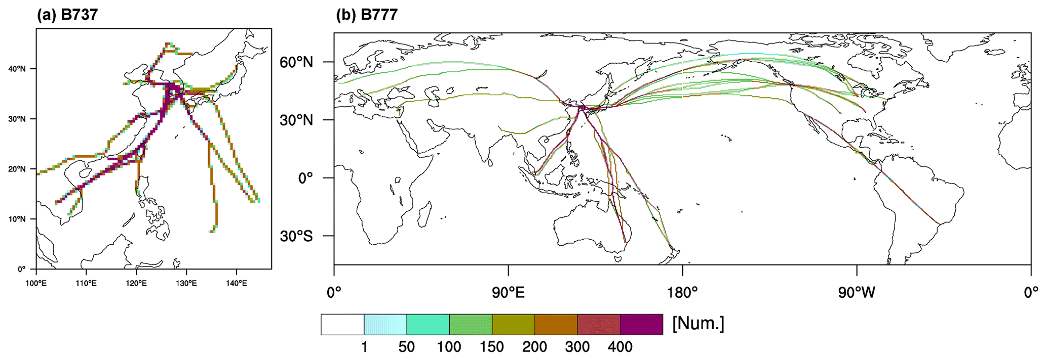
Figure 1 The horizontal distribution of the number of (a) B737 and (b) B777 aircraft data at altitudes above 15 kft, accumulated within a 0.5^∘ × 0.5^∘ horizontal grid box for the 12 months from January to December 2012.

2.2 Wind estimation

Using wind direction and wind speed of the on-board aircraft data, the zonal (U) and meridional (V) wind is computed. The vertical wind (W) is estimated as the difference between the true airspeed and the aircraft inertial vertical velocity (IVV) (e.g., Lenschow, 1972; Sharman et al., 2014):

$$\begin{array}{}\text{(1)}& \begin{array}{rl}W& =V_{\mathrm{T}}\left(\sin {\mathit{\alpha }}_{\mathrm{b}}\cos \mathit{\theta }\cos \mathit{\phi }+\sin \mathit{\beta }\cos \mathit{\theta }\sin \mathit{\phi }\right.\\ & \left.-\cos {\mathit{\alpha }}_{\mathrm{b}}\cos \mathit{\beta }\sin \mathit{\theta }\right)-\mathrm{IVV}-M\dot{\mathit{\theta }}\cos \mathit{\theta },\end{array}\end{array}$$

where V_T is the true airspeed in meters per second (m s⁻¹); α_b, θ, φ, and β are the body-axis angle of attack, the pitch angle, the roll angle, and the sideslip angle, respectively; $\dot{\mathit{\theta }}$ is the pitch rate; and M is the distance between the measurement location of the angle of attack and the aircraft center of gravity.

Given that the sideslip (β) can be negligible (Haverdings and Chan, 2010) and the rightmost term related to the pitch rate ($\dot{\mathit{\theta }})$ contributes less to the resultant EDR estimates (Sharman et al., 2014), Eq. (1) can be approximated to a simpler form (Haverdings and Chan, 2010; Sharman et al., 2014):

$$\begin{array}{}\text{(2)}& W=V_{\mathrm{T}}(\sin {\mathit{\alpha }}_{\mathrm{b}}\cos \mathit{\theta }\cos \mathit{\phi }-\cos {\mathit{\alpha }}_{\mathrm{b}}\sin \mathit{\theta })-\mathrm{IVV}.\end{array}$$

The α_b is computed from the measured right and left vane angle of attack (α_R and α_L, respectively) as

$$\begin{array}{}\text{(3)}& \begin{array}{rl}{\mathit{\alpha }}_{\mathrm{b}}& ={\mathrm{a}}_{\mathrm{0}}+{\mathrm{a}}_{\mathrm{1}}\stackrel{\mathrm{‾}}{\mathit{\alpha }}\text{and}\\ \stackrel{\mathrm{‾}}{\mathit{\alpha }}& =\left({\mathit{\alpha }}_{\mathrm{R}}+{\mathit{\alpha }}_{\mathrm{L}}\right)/\mathrm{2},\end{array}\end{array}$$

where $\stackrel{\mathrm{‾}}{\mathit{\alpha }}$ is the locally observed angle of attack that averages the α_R and α_L, and a₀ and a₁ are calibration coefficients. Since the pitch angle θ can be assumed to equal the body-axis angle of attack α_b during steady flight (Williams and Marcotte, 2000; Drüe and Heinemann, 2013; Sharman et al., 2014), Eq. (3) can be written as

$$\begin{array}{}\text{(4)}& \mathit{\theta }={\mathit{\alpha }}_{\mathrm{b}}=a_{\mathrm{0}}+a_{\mathrm{1}}\stackrel{\mathrm{‾}}{\mathit{\alpha }}.\end{array}$$

In Eq. (4), the calibration coefficients a₀ and a₁ are computed through the least-squares linear regression between θ and $\stackrel{\mathrm{‾}}{\mathit{\alpha }}$ following Sharman et al. (2014). The slope and y-axis intercept yield from the linear regression of $\stackrel{\mathrm{‾}}{\mathit{\alpha }}$ and θ are assigned to calibration coefficients a₁ and a₀, respectively. A similar approach was conducted by Williams and Marcotte (2000) and Drüe and Heinemann (2013).

Figure 2 shows scatter density plots of the measured angle of attack ($\stackrel{\mathrm{‾}}{\mathit{\alpha }})$ and aircraft pitch angle (θ), as well as linear regression fits for the B737 and B777. To objectively retrieve the intensity of atmospheric turbulence using the aircraft data (especially using derived W), the best relationship between the angle of attack ($\stackrel{\mathrm{‾}}{\mathit{\alpha }})$ and aircraft pitch angle (θ) for estimating the derived W should be found. Because two parameters (pitch angle and angle of attack) are highly sensitive to the navigation of aircraft, any data where the altitude rate is less than or equal to 10 ft s⁻¹ and the altitude is greater than or equal to 15 kft are used exclusively. Using this criterion, we found that most of the flight data (81 % of the B737 data (214 450 reports) and 94 % of the B777 data (1 004 037 reports)) are in the cruising mode of the steady flights, which are eventually used to construct the best linear regression between the angle of attack ($\stackrel{\mathrm{‾}}{\mathit{\alpha }})$ and aircraft pitch angle (θ). As a result, both B737 and B777 QAR data yield representative linear fits (a₀=3.154 and a₁=0.594 for B737 and a₀=2.096 and a₁=0.517 for B777). These calibration coefficients are used to calculate the vertical wind (W) using Eq. (2). This derived vertical wind is used to compute the EDR, together with zonal and meridional winds and the DEVG.

Figure 2 Scatter density plots (circle) of the measured angle of attack ($\stackrel{\mathrm{‾}}{\mathit{\alpha }})$ and pitch angle (θ), along with the least-squares linear regression fits (dashed line), for the (a) B737 and (b) B777. The least-squares intercept, slope, and degree of goodness of fit are written as a₀, a₁, and R², respectively.

3 EDR estimations

The EDR is estimated from 1 Hz B737 and B777 QAR data, as shown in Fig. 1 using five methods: three methods calculate the EDRs from the wind components based on the inertial dissipation method (IDM, also known as inertial range technique) (Champagne et al., 1977), and two methods estimate the EDR from the DEVG, based on the lognormal mapping scheme of Sharman and Pearson (2017) and the prescribed best-fit curve of Kim et al. (2017, 2020). Kim et al. (2020) showed that the statistical occurrence of turbulence by DEVG-derived EDRs calculated from AMDAR data is similar to that from in situ EDR measurements. Descriptions of the five methods are provided in the following sections.

3.1 EDR estimation using the IDM (EDR1, EDR2, and EDR3)

In the EDR estimation based on the IDM, Taylor's frozen turbulence hypothesis (Hinze, 1975) is invoked to express the EDR in a temporal domain. It is noted that the high true airspeed of aircraft relative to the perturbation of velocity ($u^{\prime }=u-\stackrel{\mathrm{‾}}{V_{\mathrm{T}}}$, where overbar is mean true airspeed) can hold this hypothesis to be valid ($u^{\prime }/\stackrel{\mathrm{‾}}{V_{\mathrm{T}}}\ll \mathrm{1})$. The EDR can be estimated from the three methods utilizing (i) the second-order structure function (e.g., Frehlich and Sharman, 2004), (ii) the power spectral density (PSD), and (iii) the maximum-likelihood estimation using the von Kármán spectral model (Sharman et al., 2014).

First, applying Kolmogorov's second hypothesis of similarity (Kolmogorov, 1941) and Taylor's hypothesis, the EDR can be expressed in terms of temporal increment (τ) of wind velocity, as

$$\begin{array}{}\text{(5)}& \begin{array}{r}\mathrm{EDR}={\left({\displaystyle \frac{\mathrm{1}}{\stackrel{\mathrm{‾}}{V_{\mathrm{T}}}}}\right)}^{\mathrm{1}/\mathrm{3}}{\left[{\displaystyle \frac{\stackrel{\mathrm{‾}}{D_i\left(\mathit{\tau }\right)}}{{\mathit{\tau }}^{-\mathrm{2}/\mathrm{3}}{C}_{\mathrm{K}}}}\right]}^{\mathrm{1}/\mathrm{2}}\text{and}\\ {\mathrm{D}}_i\left(\mathit{\tau }\right)=\langle {\left[u_i(t+\mathit{\tau })-u_i\left(t\right)\right]}^{\mathrm{2}}\rangle .\end{array}\end{array}$$

Here, $\stackrel{\mathrm{‾}}{V_{\mathrm{T}}}$ is the averaged true airspeed for a 2 min time window; D_i is the second-order structure function of the wind velocity component $u_i=[U,V$, and W] with a 2 min window; C_K is the Kolmogorov constant set as 0.52 for U and 0.707 for V and W (Wyngaard and Coté, 1971; Oncley et al., 1996; Strauss et al., 2015); the overbar is the arithmetic average over the predefined inertial range ($\mathrm{2}\le \mathit{\tau }\le \mathrm{5}$ s) that is about 400–1000 m of horizontal scale, considering airspeed is about 200 m s⁻¹; and angle brackets indicate an ensemble average. This is sufficiently small enough to feel atmospheric turbulent eddies that directly affect mid-size aircraft at cruising altitudes in the UTLS (e.g., Sharman et al., 2006, 2014). It is noted that the predefined inertial range is selected to minimize discrepancy between the theoretical slope and observed one for both types of aircraft, whole altitude ranges (above 15 kft), and both high- and low-turbulence regimes having the minimum size of the horizontal wavelengths.

Figure 3 shows an example of the computed second-order structure function (D_i) of meridional wind within 2 min (from 11:28 to 11:30 UTC on 11 October 2012) when strong turbulence is observed, with a change in the vertical acceleration of more than 0.8 g (g is the gravitational acceleration) and the DEVG of 5.555 m s⁻¹, which is categorized as moderate turbulence (Truscott, 2000). The structure function within the defined inertial range ($\mathrm{2}\le \mathit{\tau }\le \mathrm{5}$ s) closely follows the ${\mathit{\tau }}^{\mathrm{2}/\mathrm{3}}$ inertial range slope by the Kolmogorov turbulence hypothesis in the selected case. Although the degree of agreement between the observed wind structure functions and theoretical slope may be different case by case and according to the wind component (not shown), the observed structure functions calculated using 1 Hz QAR data represent, qualitatively, the property of turbulence within the inertial range. Finally, from this second-order structure function, the EDR can be calculated using Eq. (5), which is defined as EDR1. When the EDR is calculated from the zonal (meridional and derived vertical) wind velocity using this method, it is referred to as EDR1U (EDR1V and EDR1W, respectively).

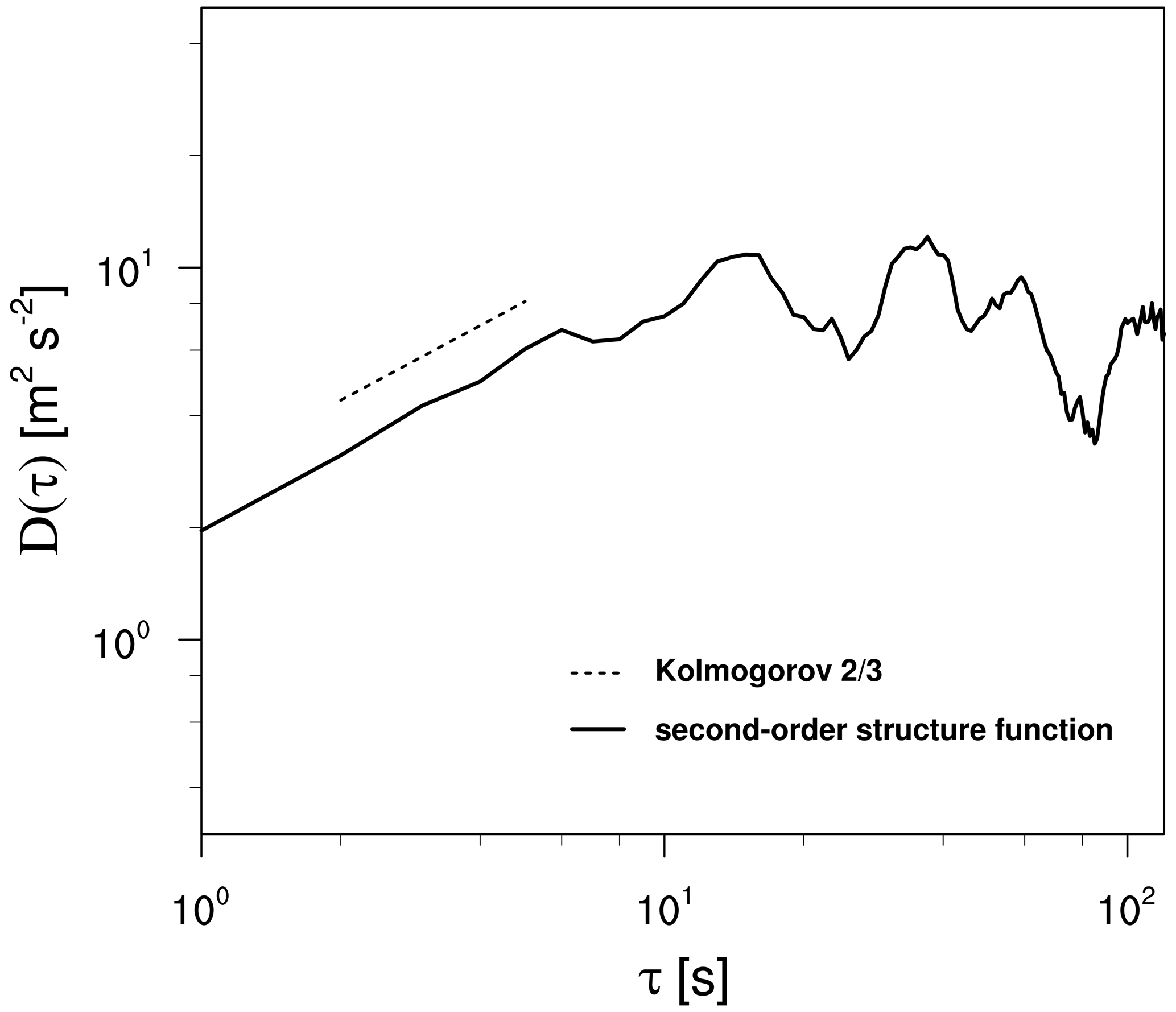
Figure 3 Example of the second-order structure functions of the meridional wind component obtained from the QAR data for 2 min (starting from 11:28 UTC on 11 October 2012) when strong turbulence (DEVG = 5.555 m s⁻¹) was observed. The dashed line represents the theoretical Kolmogorov inertial range slope ${\mathit{\tau }}^{\mathrm{2}/\mathrm{3}}$ in the time domain.

Second, the EDR can be estimated by fitting the Kolmogorov slope of $k^{-\mathrm{5}/\mathrm{3}}$ to the observed power spectral density of the wind component [S_i, ($i=U,V$, and W)] in the defined inertial range and by assuming Taylor's frozen hypothesis:

$$\begin{array}{}\text{(6)}& \mathrm{EDR}={\left({\displaystyle \frac{\mathrm{2}\mathit{\pi }}{V_{\mathrm{T}}}}\right)}^{\mathrm{1}/\mathrm{3}}\left[{\displaystyle \frac{\stackrel{\mathrm{‾}}{S_i\left(f\right)f^{\mathrm{5}/\mathrm{3}}}}{C_{\mathrm{K}}^{-\mathrm{1}}}}\right],\end{array}$$

where a range of frequency f ($f=\frac{V_{\mathrm{T}}}{\mathrm{2}\mathit{\pi }}k$, where k is wavenumber) is between 0.2 and 0.5 s⁻¹, which corresponds to the inertial range defined in Eq. (5), and the overbar is the arithmetic mean over the data within the defined inertial range. The PSD of each wind component is estimated by a fast Fourier transform (FFT) with no overlap. Before computing the FFT, the wind data are tapered using a Welch window. The resultant EDR from Eq. (6) is referred to as EDR2, and the EDR2 values from U, V, and W are labeled EDR2U, EDR2V, and EDR2W, respectively.

Third, the EDR is estimated using the maximum-likelihood estimation method (Sharman et al., 2014), which uses observed energy spectra (S_obs) and model spectra (S_model) given by

$$\begin{array}{}\text{(7)}& \mathrm{EDR}={\left({\displaystyle \frac{\mathrm{1}}{p_{\mathrm{2}}-p_{\mathrm{1}}+\mathrm{1}}}{\sum }_{f=f_{\mathrm{1}}}^{f_{\mathrm{2}}}{\displaystyle \frac{S_{\mathrm{obs}}\left(f\right)}{S_{\mathrm{model}}\left(f\right)}}\right)}^{\mathrm{1}/\mathrm{2}},\end{array}$$

where f₁ and f₂ are 0.2 and 0.5 s⁻¹, respectively, and p₁ and p₂ are the lower and upper frequency indices, respectively. The von Kármán energy spectra (von Kármán, 1948; Mann, 1994) are used as the model spectra S_model. It is noted that the observed spectrum S_obs and defined inertial range are the same as used in Eq. (6).

For zonal wind (U) data, the von Kármán wind model in the spatial domain is formulated as

$$\begin{array}{}\text{(8)}& F_{\mathrm{model}}\left(k\right)={\displaystyle \frac{\mathrm{9}}{\mathrm{55}}}\mathit{\alpha }{\mathit{\epsilon }}^{\mathrm{2}/\mathrm{3}}{\displaystyle \frac{\mathrm{1}}{({\mathrm{L}}^{-\mathrm{2}}+k^{\mathrm{2}}{)}^{\mathrm{5}/\mathrm{6}}}},\end{array}$$

where the empirical value of α is set to 1.6 (Sharman et al., 2014); L is the length scale, which is set to 669 m following Sharman et al. (2014); and ε should be unity.

For meridional wind (V) and vertical wind (W) data, the von Kármán energy spectra are formulated as

$$\begin{array}{}\text{(9)}& F_{\mathrm{model}}\left(k\right)={\displaystyle \frac{\mathrm{3}}{\mathrm{110}}}\mathit{\alpha }{\mathit{\epsilon }}^{\mathrm{2}/\mathrm{3}}{\displaystyle \frac{\mathrm{3}{L}^{-\mathrm{2}}+\mathrm{8}{k}^{\mathrm{2}}}{(L^{-\mathrm{2}}+k^{\mathrm{2}}{)}^{\mathrm{11}/\mathrm{6}}}}.\end{array}$$

Taylor's turbulence hypothesis is applied to Eqs. (8) and (9) to convert the frequency (f)-domain-based spectrum (S_model) from the spatial (k)-domain spectrum. The resultant EDR from Eqs. (7)–(9) is referred to as EDR3, and the EDR3 values derived using U, V, and W are described as EDR3U, EDR3V, and EDR3W, respectively.

We additionally conducted a sensitivity test on the inertial range. A dynamical inertial range is determined by finding the range has the minimum error between the observed power laws and theoretical one (i.e., ${\mathit{\tau }}^{\mathrm{2}/\mathrm{3}}$ or $f^{-\mathrm{5}/\mathrm{3}})$ for a given time segment. EDRs are calculated based on the three EDR estimations using the dynamical inertial range, and resultant EDRs are compared to EDRs using the predefined (fixed) inertial range. Figure 4 shows scatter density plots of the EDRs using the fixed inertial range (x axis) and dynamic inertial range (y axis) for the B777. Pearson correlation (r) and mean absolute error (MAE) between two different EDRs are also computed. It is found that there exist high correlations more than 0.97 and low MAEs between 0.001–003 m${}^{\mathrm{2}/\mathrm{3}}$ s⁻¹ between EDRs using the fixed range and dynamically selected range. For B737 (not shown), we found r = 0.93 and MAE = 0.002–0.007 m${}^{\mathrm{2}/\mathrm{3}}$ s⁻¹. In the present study, the fixed inertial range is considered, regardless of an underestimation in the magnitude of some EDRs (e.g., EDR1U and EDR1V), as it can be more computationally efficient in calculating the EDR. Further investigation, however, may be required using more and longer data in the future.

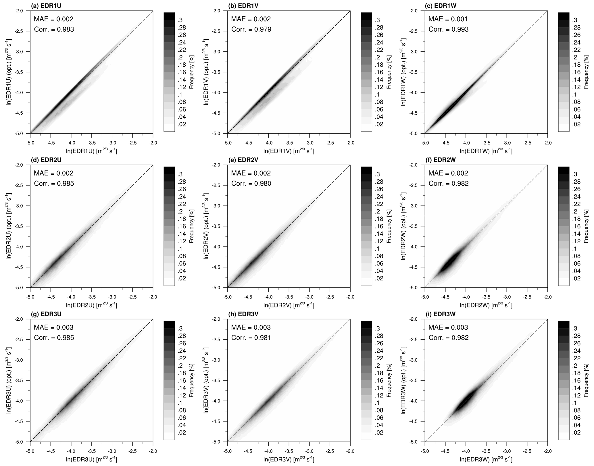
Figure 4 Scatter density plots of the EDRs – (a–c) EDR1s, (d–f) EDR2s, and (g–i) EDR3s – using the fixed inertial range and dynamic inertial range for the B777. Pearson correlation and MAE are given in the top-left corner of each panel.

The reliability of the current EDR results using the 1 Hz data is required. Unfortunately, we do not have any higher-frequency (e.g., 10 Hz) QAR data. Therefore, we applied our methods to the 20 Hz wind data obtained from the Boseong Meteorological Observatory (BMO), South Korea. For a direct comparison, raw 20 Hz wind data are subsampled to the 1 Hz wind data, and two 1 Hz datasets are created using Reynolds averaging and arbitrarily picking every middle (10th) sample. It is noted that J. Kim et al. (2021) derived EDRs using the 20 Hz BMO wind data. Three EDRs (EDR1, EDR2, and EDR3) are computed using the zonal wind of 20 and 1 Hz BMO data for early 10 d from 00:00 LST on 1 October 2019. Figure 5 shows an example of the PSDs of zonal wind obtained from the 20 and 1 Hz BMO data at 10:25 LST on 1 October 2019 at 300 m above ground level (a.g.l.) and scatter density plots of three EDRs based on U wind for 20 Hz and two different 1 Hz BMO datasets. The PSDs of 1 Hz BMO data follow a theoretical slope ($-\mathrm{5}/\mathrm{3}$), especially in the overlapped range of frequency (0.1–0.5 s⁻¹) (Figs. 5a, b). However, near the tail, part of the energy spectrum of 1 Hz wind data by selecting the arbitrary pick shows relatively larger powers (Fig. 5a) than that of averaged 1 Hz wind (Fig. 5b) and even that of the 20 Hz data (Figs. 5a, b). This is also found when every first or last (20th) samples are used (not shown), which is related to the aliasing problem and is eventually shown as relatively higher values of EDR2 and EDR3 than the averaged and original EDR values (Fig. S1 in the Supplement). This feature is not found in the structure-function-based EDR1 method (Fig. S1), which is consistent with previous study (e.g., Muñoz-Esparza et al. 2018), suggesting that the EDR1 can slightly reduce the uncertainty of retrieved EDR using the 1 Hz data. For the Reynolds averaging 1 Hz data, the retrieved EDRs are underestimated systematically regardless of the EDR methods (Fig. S1).

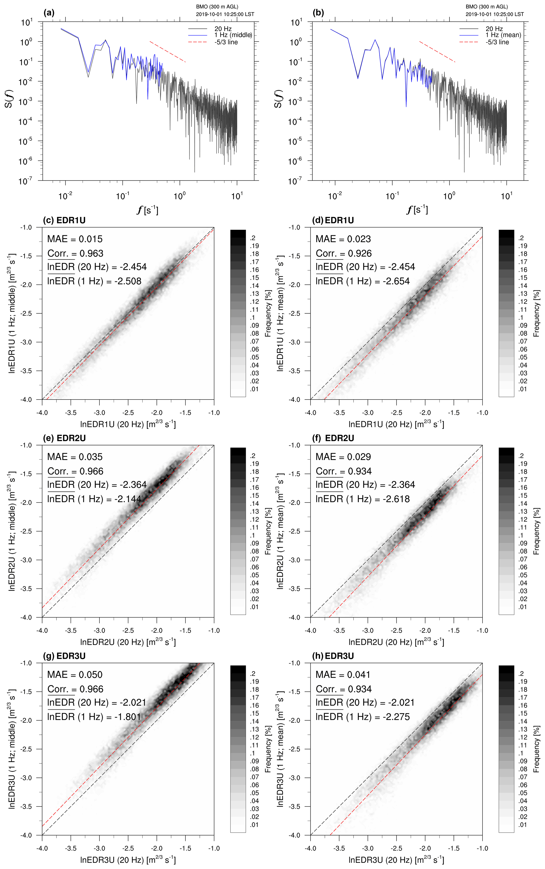
Figure 5 (a, b) The energy spectrum of the zonal wind component obtained from raw 20 Hz (black) and subsampled 1 Hz (blue) BMO data at 10:25 LST on 1 October 2019 at 300 m a.g.l. and (c–f) scatter density plots of the EDRs calculated using the 20 Hz and subsampled 1 Hz BMO data for early 10 d from 00:00 LST on 1 October 2019. Pearson correlation, MAE, and mean of the natural logarithm of EDRs calculated from 20 and 1 Hz BMO data are given in the top-left corner of Figs. 5c–f. The 1 Hz data are obtained by (a, c, e, g) picking every 10th sample from the raw 20 Hz BMO data and (b, d, f, h) Reynolds averaging the raw 20 Hz BMO data. The linear regression line is included as a red dashed line.

In scatter plots of 20 and 1 Hz EDRs from the BMO datasets, it is found that 1 Hz EDR data are highly correlated with 20 Hz EDR data (r>0.926), implying that the 1 Hz data can provide a reliable information (timing and location) of atmospheric turbulence. However, as already mentioned above, the averaging results of the 1 Hz data show the systematic underestimations of EDRs about 8.14 % (EDR1 in Fig. 5d), 10.75 % (EDR2 in Fig. 5f), and 12.56 % (EDR3 in Fig. 5h). In addition, arbitrary pick experiments have the systematic underestimations of 2.19 % in EDR1 (Fig. 5c) and the overestimations of ∼9.32 % and ∼10.91 % in EDR2 (Fig. 5e) and EDR3 (Fig. 5g) due to the aliasing problem, respectively. Given the situation that we do not know whether the 1 Hz QAR data used in this study are an averaged value or an arbitrarily picked one from the raw data, the uncertainties found in this study should be considered when we use the retrieved EDR values from the low-frequency (1 Hz) flight data for investigation turbulence encounters. Further intercomparison between 1 Hz and higher-frequency aircraft data needs to be conducted in the future.

Figure 6 shows an example of the PSD of zonal wind obtained from the QAR data at 10:38 UTC on 11 October 2012, when aircraft rarely experienced turbulence because of a change in the vertical acceleration of less than ∼0.2 g. The von Kármán and Kolmogorov theoretical $f^{-\mathrm{5}/\mathrm{3}}$ slopes for the energy spectrum, which are related to EDR2 and EDR3, respectively, are also included in Fig. 6. In general, the observed PSD follows the theoretical $-\mathrm{5}/\mathrm{3}$ slopes well. Further evaluation will be conducted through the case analysis in Sect. 4.

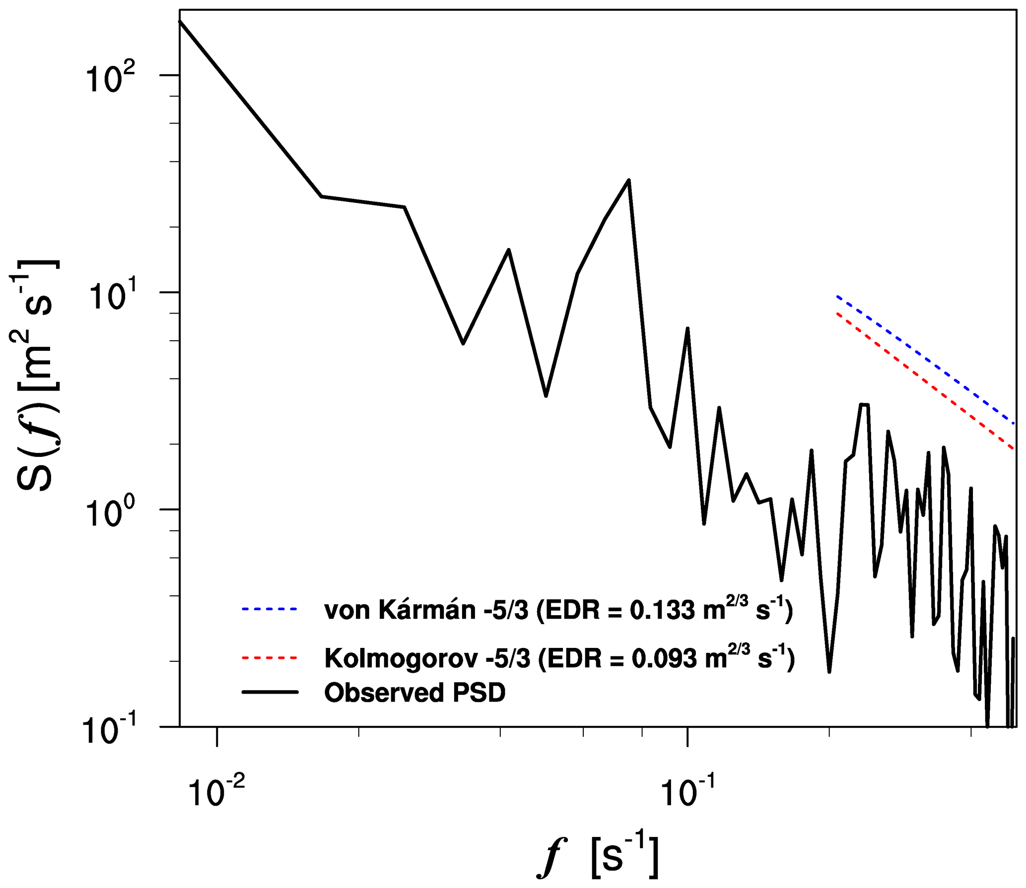
Figure 6 The energy spectrum of the zonal wind component obtained from the QAR data at 10:38 UTC on 11 October 2012. The dashed line represents the theoretical von Kármán (blue) and Kolmogorov (red) inertial range slope $f^{-\mathrm{5}/\mathrm{3}}$ in the frequency domain.

3.2 EDR conversion using the prescribed best-fit function (EDR4)

Kim et al. (2020) converted the EDR from the DEVG using the polynomial curve between the observed EDR and the DEVG constructed by Kim et al. (2017). Note that the observed EDR was computed using time series of Hong Kong-based airlines data, based on the EDR algorithm of Haverdings and Chan (2010) (Kim et al., 2017). On a one-to-one basis, Kim et al. (2017) constructed the parabolic curve between the EDR and DEVG for each type of aircraft. For the EDR conversion, Kim et al. (2020) used the best-fit curve of Boeing aircraft (B747 and B777), which have a high correlation and accuracy, as

$$\begin{array}{}\text{(10)}& {\mathrm{DEVG}}^{*}=\mathrm{0.0031}\left({\mathrm{DEVG}}^{\mathrm{2}}\right)+\mathrm{0.0286}\left(\mathrm{DEVG}\right)+\mathrm{0.0114},\end{array}$$

where DEVG^* is the remapped value to the EDR scale with units of m${}^{\mathrm{2}/\mathrm{3}}$ s⁻¹. The current study uses this best-fit curve following Kim et al. (2020) to convert the EDR from the DEVG. It is noted that the same equation (Eq. 10) is applied to both 1 Hz B737 and B777 DEVG data. The resultant EDR is called EDR4.

3.3 EDR conversion using the lognormal mapping technique (EDR5)

Considering a lognormality of turbulence discussed in many previous studies (e.g., Nastrom and Gage, 1985; Frehlich, 1992; Cho et al., 2003; Frehlich and Sharman, 2004; Sharman et al., 2014; Kim et al., 2017, 2020), Sharman and Pearson (2017) developed a lognormal mapping technique from numerical weather prediction (NWP)-based turbulence diagnostics with different physical meanings and units. This was designed such that each turbulence diagnostic climatologically corresponds to turbulence observations that follow a lognormal distribution (i.e., the random and chaotic nature of turbulence in the atmosphere). Assuming the lognormal behavior of turbulence, the simplest mapping between a raw diagnostic D and the EDR is applied as follows:

$$\begin{array}{}\text{(11)}& \begin{array}{rl}& \ln \left(D^{\ast }\right)=\ln \left(\mathrm{EDR}\right)=a+b\ln \left(\mathrm{D}\right),\\ & a=\langle \ln \left(\mathrm{EDR}\right)\rangle -b\langle \ln \left(D\right)\rangle =C_{\mathrm{1}}-b\langle \ln \left(D\right)\rangle ,\text{and}\\ & b=\mathrm{SD}\ln \left(\mathrm{EDR}\right)/\mathrm{SD}\ln \left(D\right)=C_{\mathrm{2}}/\mathrm{SD}\ln \left(D\right),\end{array}\end{array}$$

where D^* is the turbulence diagnostic remapped to the EDR scale, the angle bracket is an ensemble average, and SDln (D) and SDln (EDR) are a standard deviation (SD) of the natural logarithm of the turbulence diagnostic D and that of EDR observations, respectively. Climatological values C₁ and C₂ are set to −2.953 and 0.602, respectively, as given in Sharman and Pearson (2017) and obtained by long-term in situ EDR estimates from US-based air carriers above a 20 kft flight level. Considering that the 1-year (2012) period of the QAR data used in this study overlaps the research period (from 2009 to 2014) of the dataset used in Sharman and Pearson (2017), it is considered that the use of climatological values of Sharman and Pearson (2017) is acceptable. Although in recent days there are some efforts to update C₁ and C₂ for the low-level turbulence using high-frequency sonic anemometer mounted in the tall towers (e.g., Muñoz-Esparza et al., 2018; J. Kim et al., 2021), to our knowledge, at the present there is no recent update on C₁ and C₂ for the upper level because it requires a large number of high-frequency aircraft data for the EDR estimation. This study can be one of these efforts to provide more EDR data that are required to update C₁ and C₂ based on all available flight information including relatively low-frequency flight data such as 1 Hz post-flight data. For the EDR5, as carried out by Kim et al. (2020), the turbulence diagnostic D in Eq. (11) is replaced with the DEVG estimates (EDR5). To obtain the mean and SD of ln (DEVG), the lognormal fitting is conducted via the nonlinear least-squares fit, which uses the Levenberg–Marquardt algorithm (Moré, 1978). The data used to calculate the probability density function (PDF) are binned with the samples that are greater than 10 reports in each bin among 50 bins.

Figure 7 shows the PDFs of the DEVG in units of meters per second (m s⁻¹), computed using both the B737 and B777 QAR datasets of Fig. 1 for the same period (12 months), and lognormal fits applied to the PDFs. The largest value of the DEVG satisfying the criteria of data binning is about 3.31 and 6.18 m s⁻¹ for B737 and B777, respectively (not shown). From the lognormal fits, the mean and SD of ln (DEVG) are −2.323 and 1.031, respectively, for B737 and −2.768 and 1.180, respectively, for B777, and these values are used to calculate the EDR. As the QAR data used in the current study have only 1-year data, the seasonal and regional mean and SD are not considered. Although a one-to-one comparison to Kim et al. (2020) is difficult due to the limitations in spatiotemporal coverage, the overall magnitudes of the mean and SD of the DEVG in the current study are smaller than in Kim et al. (2020). More detailed results of comparison of PDFs with other EDR methods are given in the following sections.

Figure 7 The probability density functions (PDFs) of the DEVG and lognormal fits (line) over the DEVG for the (a) B737 and (b) B777 accumulated for the 12 months from January to December 2012.

3.4 Intercomparison of the EDR estimates

The current NWP-based turbulence forecasting methods (e.g., Sharman and Pearson, 2017; Pearson and Sharman, 2017; Kim et al., 2018; J.-H. Kim et al., 2019) use the lognormal mapping technique of Sharman and Pearson (2017) (Eq. 11 of the current study), which requires two important statistics (the mean and SD) of the observed EDR. For the mean and SD of the log-scale observed EDR (〈ln(EDR)〉 and SDln (EDR) of Eq. 11, respectively), Sharman and Pearson (2017) provided climatological values (C₁ and C₂ of Eq. 11) calculated using in situ-equipped EDR data, collected by US-based air carriers between 2009 and 2014. Similarly, with respect to turbulence research as well as aviation applications (e.g., regional turbulence forecasting), statistics of a total of 11 EDR estimates (three wind-based EDRs for U, V, and W wind components and two DEVG-based EDRs) are investigated in the current study.

Figures 8 and 9 show the PDFs and lognormal curve fits of 11 EDR estimates from the B737 and B777 archived data for 12 months from January to December 2012 (Fig. 1), respectively. Some of the lowest bins where the instrumental noise can affect some of the resulting EDR values are not used in the lognormal curve fitting (open circle). The curve fitting (line) is conducted using the Levenberg–Marquardt nonlinear least-squares fit. It is also noted that the data used in calculating the PDFs are binned with the samples with greater than 50 (15) reports in each bin among 50 bins for wind-based EDRs (DEVG-based EDRs). When other minimization methods such as Powell's method (Press et al., 1992) and Nelder–Mead simplex method (Gao and Han, 2012) are used to obtain the lognormal fit, resultant lognormal fits have a similar mean and SD to the lognormal fit from the Levenberg–Marquardt used in the current study (not shown). Some PDFs (e.g., Figs. 8g–i and 9a and g) have a higher occurrence than the lognormal fits in relatively lower bins, while most of PDFs follow the lognormal distribution in relatively higher bins. Considering limited data availability and geographical consideration, the use of longer period datasets will be required to obtain robust climatological distributions.

Figure 8 The PDFs (circle) of the EDRs and lognormal fit (continuous line) over the EDRs obtained from the B737 data. The filled circles indicate data that were used in the fit, and the open circles indicate data that are excluded from the fit. It is noted that the different range of x axis is used in each EDR.

Figure 9 As in Fig. 8 but for B777.

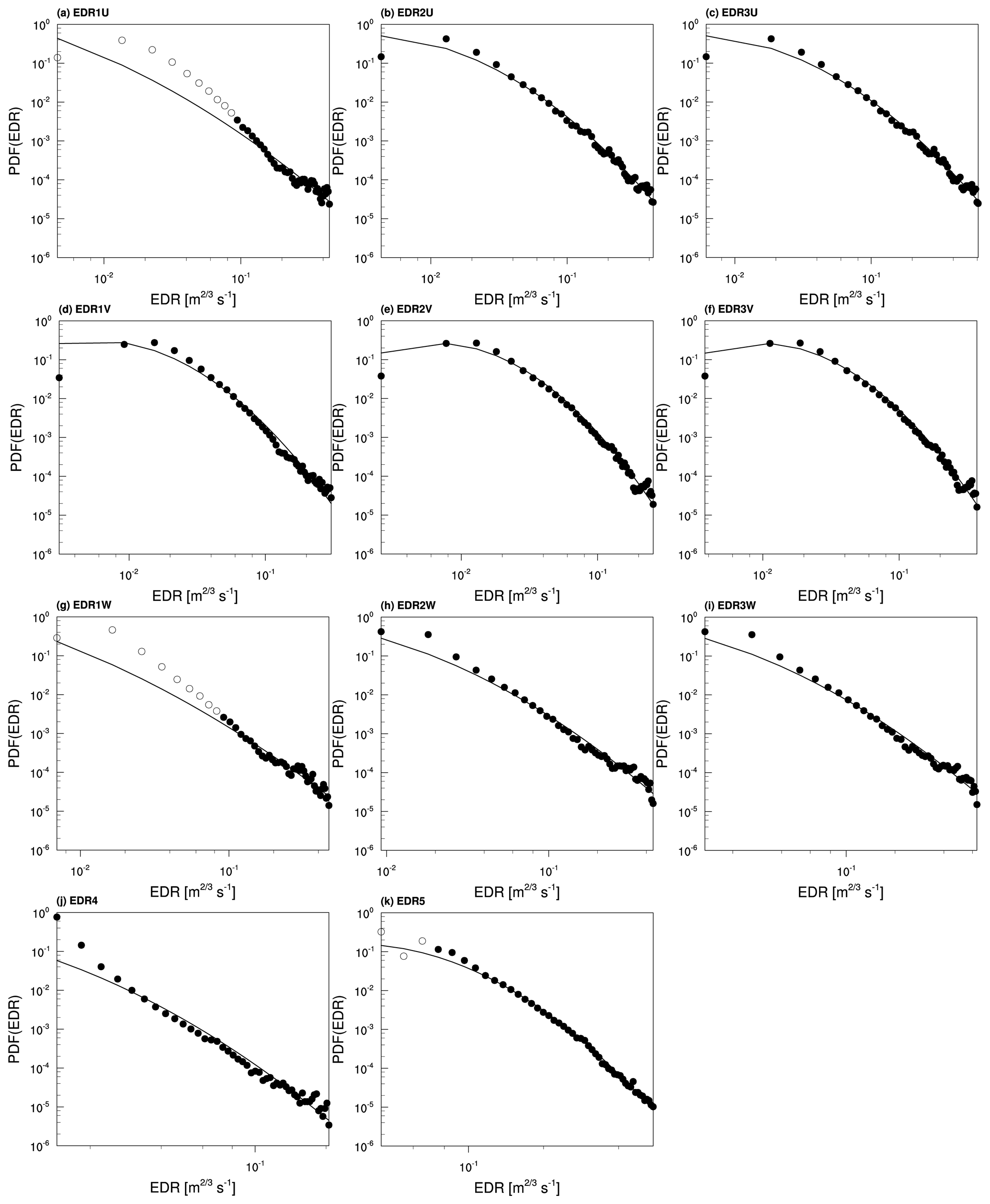
Table 1 shows the mean and SD of the natural logarithms of 11 EDRs (ln (EDR)) for each type of aircraft, which are obtained from lognormal curve fitting. Regarding the mean of ln (EDR), the B737 (from −4.75 to −2.81) is slightly larger than the B777 (from −6.31 to −2.97), and for the SD of ln (EDR), the B737 (from 0.54 to 1.17) is smaller than the B777 (from 0.62 to 1.72). For each aircraft type, the EDR estimates have similar statistics, except for EDR5. Compared to the EDR statistics (mean and SD) of previous studies (e.g., Sharman and Pearson (2017; −2.953 and 0.602, respectively), Sharman et al. (2014; −2.85 and 0.57, respectively), and Kim et al. (2020; −2.94 and 0.63 for some of Asia, respectively)), the current EDR statistics have somewhat different values, except for EDR5 (−2.81 and 0.54 for B737, respectively, and −2.97 and 0.62 for B777, respectively) and some V-wind derived EDRs (EDR1V for B737 and EDR3V for B777). This discrepancy could be due to the relatively low sampling rate of the current data, differences in the spatiotemporal coverage of data, and aircraft type. Indeed, Kim et al. (2020) showed that these statistics can vary according to specified regions (Tables 1 and 2 of Kim et al., 2020). Therefore, because the in situ-equipped EDR data cover the Northern Hemisphere (e.g., Fig. 10 of Kim et al., 2020) and miss some of the turbulence observations between Asia and Europe, between Asia and Oceania, and within Asia, the statistics, such as the mean and SD, can be different according to region and season; this remains a future research topic of interest, which could be addressed by collecting sufficient aircraft measurements. As an additional method to mitigate the imbalance of turbulence information globally, navigation information such as the ADS-B and mode-S EHS can be applied to 1 Hz based EDR estimation, together with 1 Hz aircraft measurements. Additional studies using more data and various types of aircraft data having a relatively low sampling rate of aircraft data should be conducted, in order to obtain robust statistics on the observational characteristics of turbulence.

Table 1 Values of the mean and standard deviation (SD) of the natural logarithms of EDRs computed from (a) B737 and (b) B777 QAR datasets.

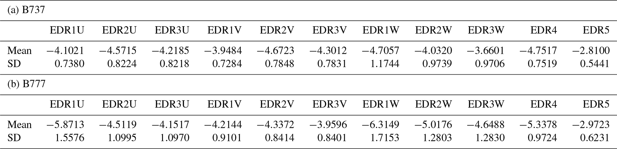
Figure 10 (a) The flight route (line) from 16:13 to 19:10 UTC on 20 September, IR image obtained from the COMS at (b) 17:15 UTC when the turbulence was encountered, (c) 16:45 UTC before the incident time, and (d) 17:45 UTC after the incident time. The horizontal location of the turbulence encounter is represented by a circle.

4 Results: case analyses

For further evaluation of the derived EDRs from the 1 Hz aircraft data in this study, the EDR estimates from five methods are examined for selected strong turbulence cases. Strong turbulence events are determined based on the DEVG values, with a threshold of 4.5 m s⁻¹ for moderate-level turbulence (e.g., Truscott, 2000; Gill, 2014; Kim and Chun, 2016; Meneguz et al., 2016; Storer et al., 2019). Therefore, time series of 11 EDR estimates, three EDR1s (U, V, and W), three EDR2s (U, V, and W), three EDR3s (U, V, and W), EDR4, and EDR5 are examined.

4.1 Convectively induced turbulence (CIT) case

Figure 10 shows the flight route between Manila, the Philippines, and Incheon, South Korea (from 16:13 to 19:10 UTC on 20 September 2012), and satellite images obtained from the infrared (IR) image of the Korean geostationary satellite, the Communication, Ocean, and Meteorological Satellite (COMS), at 18:45, 17:15, and 17:45 UTC on 20 September 2012. An aircraft heading for Incheon encountered strong turbulence, with a change in vertical acceleration of more than 1 g at an altitude of ∼37 kft near Taiwan over the Philippine Sea (121.64^∘ E and 23.05^∘ N; circle of Fig. 10) at 17:15 UTC. Around the time of this turbulence encounter (from 16:45 to 17:45 UTC), the locally isolated developing convective cloud was collocated at the region of the turbulence encounter. When the minimum IR brightness temperature (T_b) is calculated near the location of the turbulence encounter using 3-hourly GridSat-B1 data with a spatial resolution of 0.07^∘ (Knapp et al., 2011), it is found that the minimum T_b is the lowest at 18:00 UTC, which is the closest time with the turbulence encounter (not shown). This implies a rapid increase in cloud top height and corresponds well to the satellite images of Fig. 10. Therefore, we consider that this case is associated with turbulence above the rapidly developing isolated convection possibly with convectively induced gravity waves (e.g., Lane and Sharman, 2008; Kim and Chun, 2012; S.-H. Kim et al., 2019; Lane et al., 2003, 2012).

Figure 11 shows the time series of flight altitude, the DEVG, and 11 EDR estimates obtained from the 1 Hz QAR data on 20 September 2012. In Fig. 11a, a very strong and isolated peak of a large DEVG value (maximum value of 8.067 m s⁻¹) was found near the eastern side of Taiwan (circle of Fig. 10) at ∼37 kft flight level. At that time, a high rate of change in altitude of 12.5–22 ft s⁻¹ occurs (not shown). For this case, the time series of EDR estimates using each wind component (EDR1, 2, and 3) are examined separately (Fig. 11b–d). Note that the EDR4 and EDR5 in Fig. 11b–d are the same, because they do not use the wind data. A total of 11 EDRs exhibit the isolated peak and similar pattern to the vertical acceleration-based DEVG, although there are some differences in the EDR magnitudes. Among the wind-based EDRs (EDR1, 2, and 3), the EDR values estimated from the derived vertical wind velocity (W) are much larger than those from the zonal and meridional wind velocity (U and V). The largest values of EDRs derived from W (EDR = 0.739 m${}^{\mathrm{2}/\mathrm{3}}$ s⁻¹) could be relevant to rapidly developing small-scale convection, which normally includes strong updrafts and flow deformation at the top of cloud and generates subsequent convectively induced gravity waves above the convection with small-scale turbulent mixing near the top of convection (e.g., Lane and Sharman, 2008; Kim and Chun, 2012; S.-H. Kim et al., 2019; Lane et al., 2003, 2012). And, considering that the intensity criteria of light, moderate, and severe turbulence for mid-size aircraft such as the B737 are 0.15, 0.22, and 0.34 m${}^{\mathrm{2}/\mathrm{3}}$ s⁻¹ of EDR (Sharman and Pearson, 2017), the EDRs represent strong turbulence (severe turbulence), except for the EDRs derived from U (null or light intensity) and the EDR2 derived from V (moderate turbulence). The EDRs derived from W indicate that this was an extremely severe intensity and highly localized turbulence at the time that the turbulence event was observed.

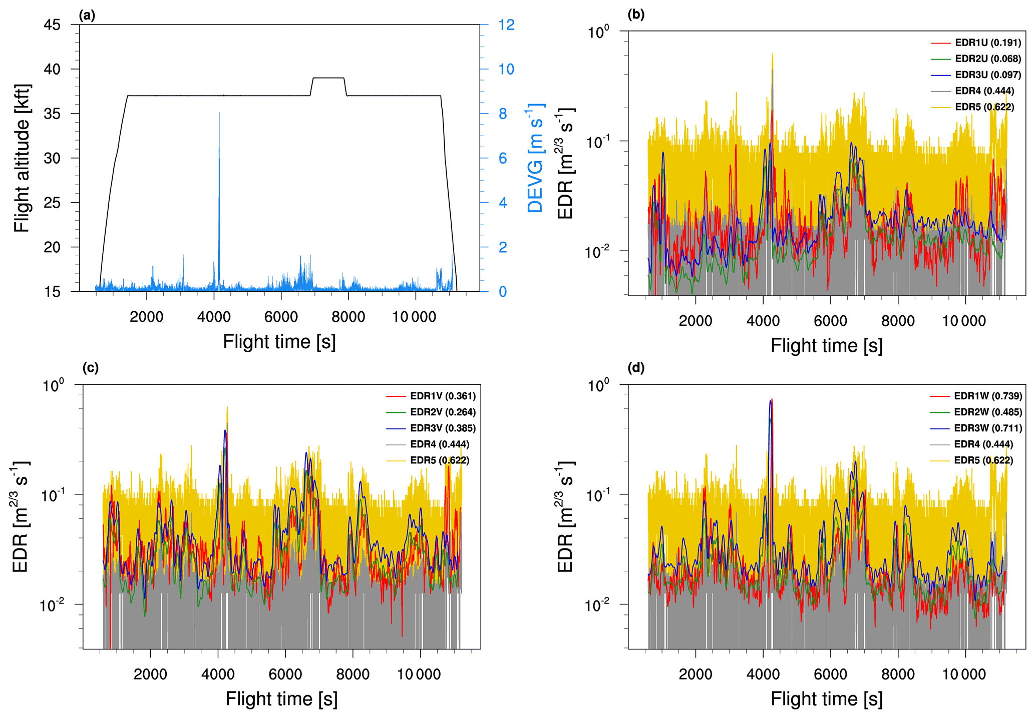
Figure 11 Time series of (a) flight altitude and DEVG and (b–d) EDR estimates obtained from the QAR data on 20 September 2012. The maximum value of the EDR is written in parentheses.

4.2 Clear-air turbulence (CAT) case

Figure 12 shows two flight routes between Incheon and Seattle (route 1: from 09:42 to 18:36 UTC) and between Incheon and San Francisco (route 2: from 08:30 to 17:42 UTC) on 11 October 2012. Figure 12 also shows the observed IR T_b (Fig. 10a), 200 and 250 hPa horizontal wind speed and vector (Fig. 10b and c, respectively), and 225 hPa vertical wind shear (Fig. 10d), computed using the European Centre for Medium-Range Weather Forecasts Reanalysis, version 5 (ERA-5, Hersbach et al., 2020), reanalysis data with a horizontal grid spacing of 0.25^∘ at 12:00 UTC on 11 October 2012. The observed T_b is obtained from the GridSat-B1 data, with the horizontal grid spacing of 0.07^∘ (Knapp et al., 2011). Two aircraft flying along both flight routes encountered strong turbulence with an abrupt change in vertical acceleration of ∼0.74 g at an altitude between 35 and 37 kft, over the northwestern Pacific Ocean (146.19^∘ E and 37.46^∘ N at 11:25 UTC for route 1 and 145.59^∘ E and 37.19^∘ N at 10:10 UTC for route 2). At that time, the intensified Typhoon Prapiroon was located in the Philippine Sea, which brought warm and moist southwesterly flows to the incident locations, while an intensified upper-level trough in the mid-latitude provided a strong northwesterly, which brought increased meridional temperature gradients and provided favorable conditions for strong vertical wind shear via the thermal wind relationship with a high wind speed at the tropopause level over the turbulence regions (e.g., Kim and Chun, 2010, 2011; Williams and Joshi, 2013; Lee et al., 2019). Near the incident locations (shown as black open circles in Fig. 12b–c), the horizontal wind speed at 200 hPa (Fig. 12b) is stronger than 70 m s⁻¹, which is almost 25 m s⁻¹ higher than that at 250 hPa (Fig. 12c). This caused strong vertical shear of zonal winds between the 200 and 250 hPa levels in the upper-level jet (Fig. 12d), which results in shear instability to generate small-scale turbulence directly affecting cruising aircraft near the turbulence locations (e.g., Kim and Chun, 2010, 2011, 2016; Kim et al., 2011, 2018; Sharman and Lane, 2016; Storer et al., 2019). This case is considered as a conventional type of CAT due to the shear instability in the upper-level jet, although turbulence events were reported over the cloud, which seems to have a relatively broad T_b, like a cirrus cloud (Fig. 12a).

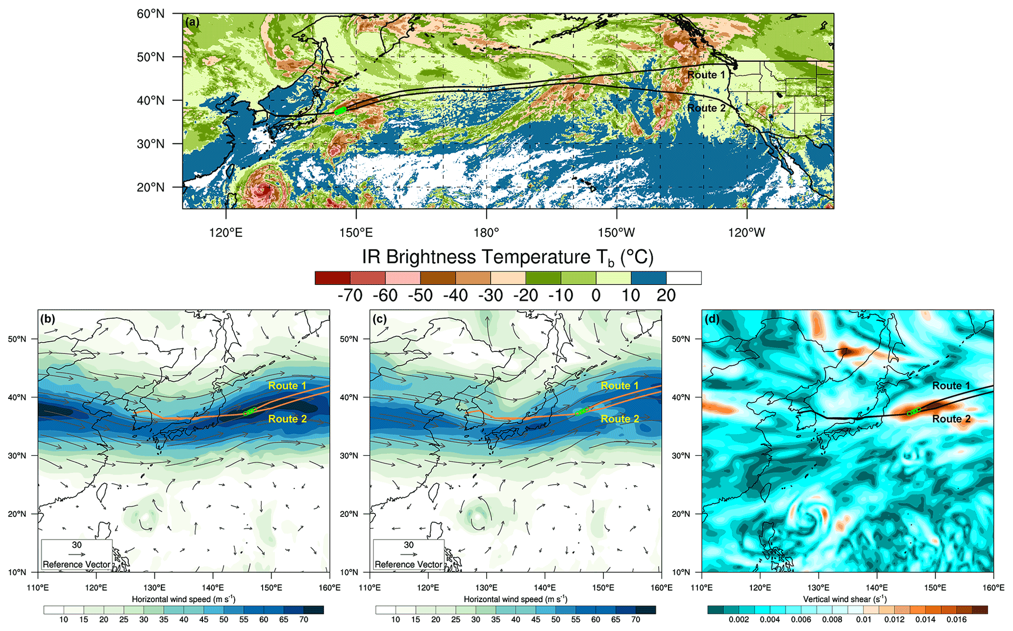
Figure 12 (a) Observed infrared brightness temperature and (b, c) horizontal wind speed (shading) and wind vector (curly arrow) at 200 and 250 hPa, respectively, and (d) vertical wind shear at 225 hPa computed from the ERA-5 reanalysis data at 12:00 UTC on 11 October 2012. The flight routes (line) and horizontal locations (circle) of MOG-level turbulence events from two QAR datasets (routes 1 and 2: from 09:42 to 18:36 UTC and from 08:30 to 17:42 UTC, respectively) are superimposed.

Figure 13 As in Fig. 11 but for (a–d) route 1 and (e–h) route 2 of the QAR data on 11 October 2012.

Figure 13 shows the time series in the same format as in Fig. 11, except for the CAT cases on 11 October 2012 (Fig. 12a–d for route 1 and Fig. 12e–h for route 2). At the time of turbulence occurrence, there are abrupt increases in the DEVG of 6.48 m s⁻¹ (route 1) and 10.75 m s⁻¹ (route 2) (Fig. 13a). At that time, the high rate of the altitude changed by more than 18 ft s⁻¹ for both flight routes (not shown). Contrary to Fig. 11, with an isolated peak, the time series of DEVG for both routes 1 and 2 had more variations before and after the turbulence incident, especially route 1 (Fig. 13a). As found in Fig. 11, the EDR estimates feature the strong CAT occurrence, and the temporal patterns of the EDR estimates and the DEVG are similar to each other. However, the EDR values derived from U are larger than those from V and W. Considering turbulence cases located in the regions of the dominant upper-level jet stream, larger-scale disturbance, such as a jet stream, can greatly affect turbulence generation (Cho and Lindborg, 2001), and this may lead to higher values of EDR from the zonal wind component than that from other wind components. The EDR derived from W also has the second largest value, and this can be relevant to the spontaneous imbalance and emission of inertial gravity waves induced by the jet stream (Knox et al., 2008). Moreover, the EDRs indicate MOG-level turbulence (EDR ≥ 0.22 m${}^{\mathrm{2}/\mathrm{3}}$ s⁻¹), except for the EDR2 and EDR3 from V and EDR4. It is noteworthy that the EDR estimates from the V-wind component are significant and highly variant from different methods, because this case is related to the Kelvin–Helmholtz billows due to strong shear instability which causes a strong y component of vorticity (vortex tube; Clark et al., 2000; Kim and Chun, 2012).

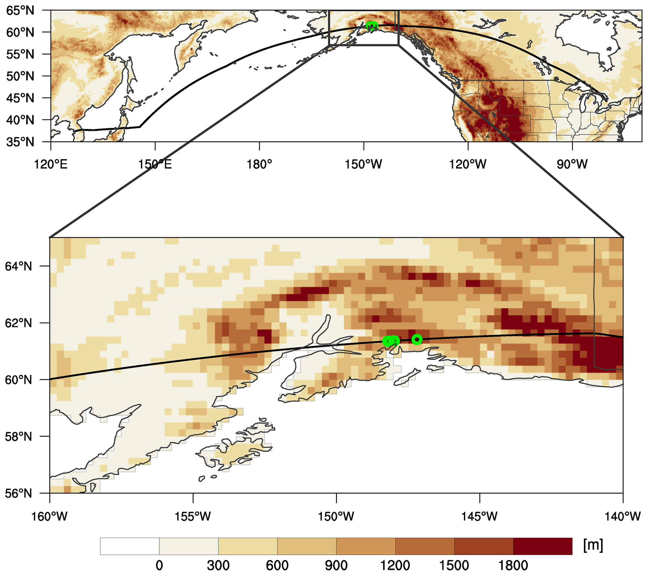
Figure 14 Flight route (line) and horizontal locations (circle) of MOG-level turbulence events detected from the QAR data on December 2012 (from 02:53 to 15:07 UTC on 30 December), with a horizontal distribution of terrain height of 5 min digital elevation model data.

4.3 Mountain wave turbulence (MWT) case

Figure 14 shows the flight route between Incheon and Toronto (from 02:53 to 15:07 UTC on 30 December 2012) and the terrain height obtained using 5 min digital elevation model data. Aircraft heading to Toronto Pearson International Airport encountered strong turbulence, with a change in the vertical acceleration of more than 1.3 g between 10:12 and 10:16 UTC at an altitude of ∼33 kft over Alaska (148–148.2^∘ W and ∼61.36^∘ N), where low-level wind and upper-level wind jet streams existed (not shown). Therefore, the MWT case could be relevant to synoptic-scale phenomena (Sharman and Pearson, 2017), and at the incident locations, the terrain height is locally steepened. This is clearly indicated in the zoomed-in field of Fig. 14. Indeed, Alaska has been considered as a representative mountain wave area (e.g., Sharman and Lane, 2016). In this regard, although we need further investigation of the generation, propagation, and breaking of mountain waves in this case, this case can be related to mountain waves and their subsequent breakdown, which is one of the well-known turbulence sources (Kim and Chun, 2010, 2011, 2016; Sharman and Pearson, 2017; Kim et al., 2018).

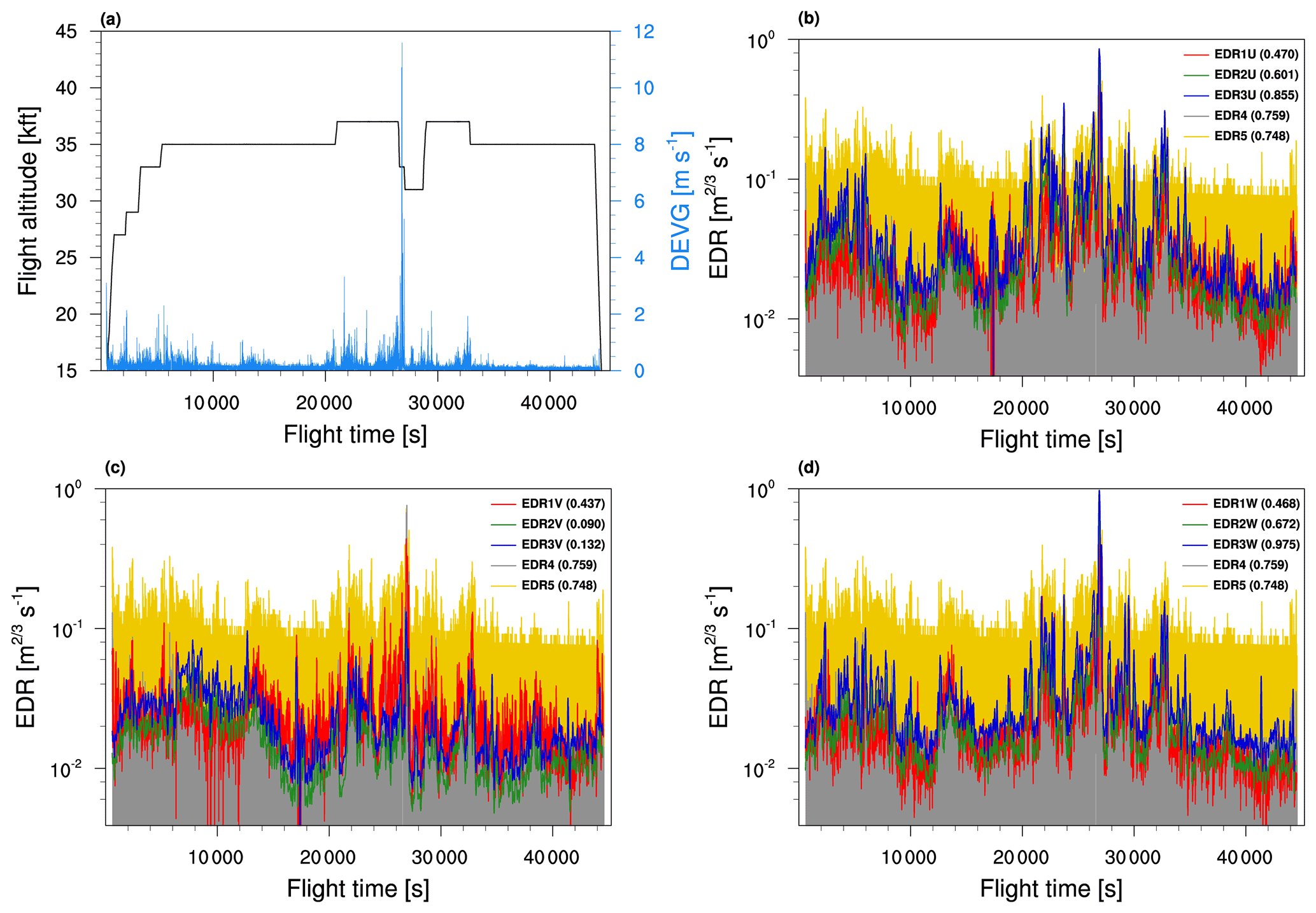
Figure 15 shows the time series that are the same format as in Fig. 11, except for the MWT case on 30 December 2012. The DEVG recorded large values of more than 11 m s⁻¹ several times (Fig. 15a). As in Fig. 13, the DEVG shows more variations before and after the peak than the CIT case. Among the three cases (CIT, CAT, and MWT cases), the MWT case had the largest variation of vertical acceleration and the largest magnitude of the resultant DEVG. For 4 min, the aircraft collected eight MOG-level (four severe and four moderate) turbulence reports. This implies that the scale of sources (synoptic-scale) for CAT and MWT is different from that for CIT (isolated mesoscale convective cell). The DEVG-based EDRs are more than 0.7 m s⁻¹, which corresponds to severe turbulence based on Sharman and Pearson (2017). As shown in Figs. 11 and 13, the EDR estimates capture the MWT occurrences well, and the patterns of EDR estimates are similar to each other. However, in the MWT case, the EDR derived from W is larger than that from U and V. As the aircraft flew above the mountainous regions, vertically propagating gravity waves may have perturbed the background conditions and led to an environment conducive to turbulence generation. Furthermore, mountain wave amplification and its subsequent breaking lead to small-scale turbulent mixing directly. A bumpy ride caused by mountain waves can be related to the large values of the EDR estimates from both the U and W wind components. Like Fig. 13, the EDRs indicate severe turbulence (EDR ≥ 0.34 m${}^{\mathrm{2}/\mathrm{3}}$ s⁻¹), except for the EDR2 and EDR3 from V. The current study examines the feasibility of using 1 Hz EDR estimates for strong (MOG-level) turbulence cases that are related to CIT, CAT, and MWT. We found that a total of 11 EDR estimates capture well the turbulence cases generated by different mechanisms, in terms of both their intensity and temporal patterns. It is also noteworthy that the characteristics of EDRs vary depending on sources of turbulence. As far as we know, there is no work done to compare the accuracy of EDR among the EDR estimation methods in the different synoptic and mesoscale regimes, which needs further investigation in the future.

Figure 15 As in Fig. 11 but for the QAR data on 30 December 2012.

5 Summary and discussion

In the current study, we derive the EDR using a relatively low sampling frequency (1 Hz) of aircraft measurements compared with a relatively high sampling frequency (e.g., 8 or 10 Hz) of in situ EDR measurements. We use the retrieved 1 Hz QAR data of the B737 and B777 for 12 months (January to December 2012) obtained from KA post-flight recorders. The wind (zonal, meridional, and vertical wind) information and the DEVG are used to compute the EDR separately. The vertical wind data that were not included in the QAR dataset are estimated using some flight parameters, such as the angle of attack, inertial vertical velocity, and roll angle. Three wind components are used to calculate three different EDRs, utilizing the structure function, PSD, von Kármán wind model, and maximum-likelihood method-based EDR estimation, under the assumption of Taylor's frozen hypothesis. Two DEVG-based EDRs are also computed using the prescribed parabolic curve proposed by Kim et al. (2017) and lognormal mapping technique proposed by Sharman and Pearson (2017).

We applied our methods to the 20 Hz wind data obtained from the BMO and subsampled 1 Hz wind data using both Reynolds averaging and arbitrary selection of every 10th sample. It is found that when the lower-rate (1 Hz) data are used to estimate the EDR, 1 Hz data have high correlation with the higher-rate data, which implies that 1 Hz data can be feasible to detect reliable timing and location of the turbulence. However, it is also found that there is a systematic underestimation (2.19 %–10.75 %) or overestimation (9.32 %–10.91 %) in the resultant EDR values compared to the higher-rate (20 Hz) data. When we use the retrieved EDR values from the low-frequency (1 Hz) flight data for investigating turbulence encounters, the uncertainties found in this study should be considered. And, given that the PSDs of 1 Hz data are sensitive depending on the way of creating 1 Hz data (averaging or arbitrary pick) together with the potential aliasing problem, it is also considered that the EDR1 can be a more stable approach to estimate the EDR than the EDR2 and EDR3 when the 1 Hz data are used.

Using these five methods (three wind-based and two DEVG-based methods), the 11 EDR estimates are computed for each type of aircraft, and the results are tested to objectively measure the feasibility of turbulence detections associated with various sources of turbulence events. The findings are summarized as follows.

1. It is found that 1 Hz EDR estimates exhibit good agreement with selected MOG-level turbulence events, with respect to turbulence intensity and temporal patterns that are related to CAT, MWT, and CIT, with different characteristics of the observed EDRs.

2. Zonal (vertical) wind-based EDRs are stronger in the CAT (CIT) case, while MWT has the peak of EDRs in both zonal and vertical wind-based EDRs.

3. Most of EDR estimates from the five different methods follow the lognormal distribution in relatively higher bins, where some PDFs tend to indicate a higher occurrence than the lognormal PDFs in relatively lower bins.

4. The statistics (mean and standard deviation) of log-scale EDRs are somewhat different from those of a previous study using a higher frequency (e.g., 8 or 10 Hz) of in situ aircraft data in the US, likely due to different sampling rates, aircraft types, locations, and limited time period.

This can contribute to expand more EDR information at the cruising altitudes in the world, which is helpful to provide more opportunities to objectively evaluate the turbulence forecast system with lower-frequency QAR and/or other in situ aircraft observation data such as ADS-B in the future. The results in the case studies also strongly suggest that the observed EDR estimates derived from different wind components such as U, V, and W can show different characteristics depending on the potential sources of atmospheric turbulence in the cruising altitudes (UTLS). This is of interest because it can provide basic information for the classification of the recent in situ EDR from the aircraft-based observation (ABO) data that are useful for producing a better climatology of upper-level turbulence and turbulence forecast systems (e.g., Sharman et al., 2006; Kim et al., 2011, 2018; J.-H. Kim et al., 2019; S.-H. Kim et al., 2021; Kim and Chun, 2016; Sharman and Pearson, 2017).

This study does not show that the different EDR methods show different characteristics of the observed EDR. When using all available methods to estimate EDR using 1 Hz data, it is found that there is no significant difference depending on the different EDR methods. However, this study emphasized that the different EDR values from various wind components (U, V, and W) show significantly different characteristics in the same EDR method. As shown in the current case analyses, the characteristics of the EDR observations from different wind components are highly dependent on the sources (CIT, CAT, and MWT) of turbulence in the UTLS. This can be eventually useful for situational awareness of cruising aircraft and tactical avoidance for turbulence, as well as producing a better climatology of turbulence classification. For the situational awareness of cruising aircraft and tactical avoidance of turbulence, we found that the CAT and MWT cases that occurred due to large-scale (synoptic-scale) forcing have longer variations in the observed EDRs before and after the turbulence incident, while the CIT case triggered by a smaller-scale mesoscale convective cell has an isolated (highly localized) peak of EDR. This feature could be useful for pilots to take more proactive action to turn on the seat belt sign before the CAT and MWT are expected to happen. If they consider that CAT is more likely to be concentrated in a shallow layer above or below the jet core (like a pancake), they can avoid these areas by only changing the altitudes for the CAT cases confirmed by strong U-wind variations in the on-board parameters.

For a better climatology of turbulence classification, up to now we have three different types of turbulence in atmosphere: CAT, MWT, and CIT (e.g., Sharman et al., 2006; Kim et al., 2011, 2018; J.-H. Kim et al., 2019; S.-H. Kim et al., 2021; Kim and Chun, 2016; Sharman and Pearson, 2017). For a better forecasting system, we need a better climatology or classification of the observed EDR estimations based on these three possible sources. This study firstly reported that the observed EDR estimates from three wind components (U, V, and W) in the 1 Hz ABO data can show significantly different characteristics. Those features are summarized as follows.

1. CAT has a string variation in zonal wind, because it is affected by large-scale forcing such as an upper-level jet/frontal system (e.g., Dutton and Panofsky, 1970; Ellrod and Knapp, 1992; Kim and Chun, 2010) and geostrophic imbalance with emissions of inertial gravity waves with the larger horizontal wavelengths (e.g., Lane et al., 2004; Zhang et al., 2004; Koch et al., 2005; Knox et al., 2008; Ellrod and Knox, 2010).

2. MWT has a large variation in both zonal and vertical wind in this study. There are two reasons for this. First, vertically propagating mountain waves are highly driven by large-scale flows across the mountain (e.g., Lane et al., 2009). Second, large amplitudes of mountain waves and their subsequent breaking are revealed by strong magnitudes of vertical velocity fields (e.g., Kim and Chun, 2010; Sharman et al., 2012).

3. CIT has highly transient and localized features in the derived vertical velocity, because it is related to convectively induced gravity waves outside the cloud boundary (e.g., Chun and Baik, 1998; Lane et al., 2003; S.-H. Kim et al., 2019, 2021) or strong updraft/downdraft inside the cloud (e.g., Lane et al., 2003; Kim and Chun, 2012). In summary, CAT, MWT, and CIT cases in this study have different characteristics in the observed EDR estimations based on U, V, and W.

Although more case analyses need to be required in the future, current results can be a useful reference for a situational awareness of cruising aircraft and for producing a better climatology. This test can be extended by applying these EDR estimation methods to the 1 Hz real-time data in the future, which can be eventually useful for a better awareness of atmospheric conditions for cruising aircraft. Possible candidates for the 1 Hz real-time data are the navigational information of commercial aircraft such as the ADS-B and mode-S EHS. Given that the setup for the ADS-B or mode-S EHS receiving stations does not require a lot of work or money for transmission of the data, EDR estimates from ADS-B and mode-S EHS (e.g., Krozel and Sharman, 2015; Kopeć et al., 2016) could greatly support the construction of a turbulence database and statistics globally, together with on-board-based (both fine and coarse) EDR measurements (e.g., Sharman et al., 2014; Gill, 2014) and other sources of data like radiosonde, weather radars, and lidars (e.g., Bodini et al., 2019; Ko et al., 2019; J.-H. Kim et al., 2021; J. Kim et al., 2021).