Quantifying the coastal urban surface layer structure using distributed temperature sensing in Helsinki, Finland

The structure of the urban boundary layer, and particularly the surface layer, displays significant complexity, which can be exacerbated by coastal effects for cities located in such regions. Resolving the complexity of the coastal urban boundary layer remains an important question for many applications such as air quality and numerical weather prediction. One of the most promising new techniques for measuring the structure of the surface layer is fibre-optic distributed temperature sensing (DTS), which has the potential to provide new significant insights for boundary layer meteorology by making it possible to study thermal turbulence with high spatial and temporal resolution.

We present 14 weeks of profile measurements with a DTS system at an urban site in Helsinki, Finland, during the winter and spring of 2020. We assess the benefits and drawbacks of using DTS measurements to supplement sonic anemometry for longer measurement periods in varying meteorological conditions, including those found difficult for the DTS method in prior studies. Furthermore, we demonstrate the capabilities of the DTS system using two case scenarios: a study of the erosion of a near-ground cold layer during the passage of a warm front, and a comparison of the near-ground thermal structure with and without the presence of a sea-breeze cell during springtime convective boundary layer development.

This study demonstrates the utility of DTS measurements in revealing the internal surface layer structure, beyond the predictions of traditional surface layer theories. This knowledge is important for improving surface layer theories and parametrisations, including those used in numerical weather prediction. The study also highlights the drawbacks of DTS measurements, caused by low signal-to-noise ratios in near-neutral atmospheric conditions, especially when such a system would be used to supplement turbulence measurements over longer periods. Overall, this study presents important considerations for planning new studies or ongoing measurements utilising this exciting and relatively new instrumentation.

1 Introduction

The atmospheric boundary layer (ABL) is a dynamically and structurally complex layer directly influenced by the surface characteristics of the Earth and which controls the interaction between the surface and the atmosphere. Due to the turbulent nature of the ABL, it has remained notoriously difficult to study and theoretically describe. This applies especially to the urban boundary layer (UBL), a subtype of the ABL, where human influence has a high impact, with surface characteristics heavily modified compared to natural surfaces (Barlow, 2014). The vertical structure of the UBL is strongly influenced by an increase in the surface roughness due to buildings and other structures and the additional anthropogenic heating coming from sources such as buildings and traffic. The UBL can be considered to be an internal boundary layer (IBL) that forms in conjunction with surrounding surfaces with different surface characteristics. This is especially the case where there are sharp borders between different surface types, such as coastal urban areas. The presence of an IBL causes spatial generalisation loss for point-like in situ measurements, as they represent only the specific IBL that the measurement instrument is located within.

In the lowest part of the UBL, the flow and turbulence are strongly influenced by the surface. This layer is the roughness sublayer (RSL), and in some situations this can be deep enough that it extends up to the surface layer top, preventing an inertial sub-layer (ISL) from forming (Rotach, 1999; Cheng et al., 2007). Instruments for measuring the ABL structure are commonly installed within the ISL in order for them to be representative of the urban surface. Understanding the structure of the RSL and possible ISL above are fundamental for several meteorological applications such as pollutant transport and wind conditions.

A vast number of in situ and remote sensing observational methods have been utilised in ABL research over the years. Since the 1990s and early 2000s, sonic anemometers have formed the modern in situ backbone of micrometeorological studies (Aubinet et al., 2012). Sonic anemometers, by their capability of providing both the three-dimensional wind components and sonic temperature at high frequency, are particularly suited to providing surface fluxes using the eddy covariance (EC) method. However, sonic anemometry, like other point-like in situ methods, lack the desired spatial coverage unless multiple instruments are deployed. Deploying multiple instruments increases however the total cost of the system and thus have been rarely applied. Additionally, especially for horizontal setups, flow distortion by the instrumentation and their supporting structures adds a limit to the number of instruments that can be reasonably used. Therefore, methods that can provide better spatial and vertical coverage with fewer instruments and with less supporting structures can prove highly beneficial for ABL studies (Foken, 2017). This is especially true for RSL studies, where the inhomogeneous nature of turbulence requires detailed spatial coverage.

One increasingly utilised approach to provide three-dimensional spatial coverage of the ABL is to use ground-based remote sensing methods. Ceilometers provide information on the evolution of the boundary layer structure (Kotthaus et al., 2020), whereas scanning Doppler lidar can provide the wind profile (Päschke et al., 2015) and the turbulence structure (Manninen et al., 2018) in addition to the ABL depth (Tucker et al., 2009). These techniques provide great value for ABL studies but they commonly lack information on the RSL due to limitations on their resolution and the lowest altitude from which measurements are possible (Emeis, 2011). Other remote sensing instruments utilised in urban ABL studies include sodar (Bradley et al., 2015) and scintillometers (Ward, 2017); however, finding appropriate locations in urban areas can be challenging.

One of the most promising new techniques for measuring the structure of the ABL is fibre-optic distributed temperature sensing (DTS) (e.g. Selker et al., 2006; Tyler et al., 2009; Thomas et al., 2011). In a DTS system, laser pulses of a specific wavelength are sent from an instrument through an optical fibre. Some of this light is scattered within the fibre due to imperfections, but also due to the non-crystalline structure of glass. This scatter is composed of Rayleigh, Brillouin, and Raman scatter. Raman backscattering is when the material (here the fibre) absorbs and then re-emits photons at a different wavelength to the transmitted wavelength; Stokes scattering refers to photons emitted at longer wavelengths; and anti-Stokes scattering refers to photons emitted at shorter wavelengths. The intensity of anti-Stokes scattering depends on temperature, whereas Stokes scattering is independent of temperature. Through this temperature dependency of the anti-Stokes signal, it is possible to derive the temperature of the fibre at high frequency and to provide along-fibre resolution using the time of flight with very short laser pulses (Selker et al., 2006).

DTS has already been used in a growing number of studies of the surface layer, including one-dimensional profile measurements of temperature (Keller et al., 2011; Higgins et al., 2018; Fritz et al., 2021; Peltola et al., 2021) and studies with two- or three-dimensional arrays (Thomas et al., 2011; Zeeman et al., 2015; Pfister et al., 2017, 2019; Mahrt et al., 2020). Furthermore, by using heated or wetted cables, DTS can be used to study wind speed (Sayde et al., 2015) or humidity (Schilperoort et al., 2018; Izett et al., 2019). However, up to now, most studies have spanned only a few days or a few weeks at maximum, and have generally focused on specific research questions well suited for the technique. The performance of the DTS method for longer campaigns or continuous measurements has not been previously assessed. Various meteorological conditions can be challenging for DTS, as the method requires a relatively high amount of thermal turbulence to provide reliable estimates of thermal turbulence statistics (Peltola et al., 2021). Solar radiation can also induce an error in the measurements (de Jong et al., 2015), as does wetting of the cable due to precipitation or fog (Izett et al., 2019). These hinder the possibility that DTS can be used to supplement, for example, eddy covariance (EC) instrumentation. Therefore, it is important to study the behaviour and performance of the method to better understand its suitability for supplementing further ABL studies.

This article presents an overview of 14 weeks of profile measurements with a DTS system at an urban site in Helsinki during the winter and spring of 2020. The main aims are to assess the benefits and drawbacks of DTS measurements for longer measurement periods in varying meteorological conditions, and to demonstrate the usefulness of temperature profile measurements with DTS in a coastal surface layer beyond traditional turbulence statistics estimation using two case studies. The first case study investigates the erosion of a near-ground cold layer during the passage of a warm front. The second case study compares the near-ground thermal structure with and without the presence of a sea-breeze cell during springtime convective boundary layer (CBL) development. We demonstrate multiple ways of extracting useful information from the DTS measurements in varying environmental conditions, including those which could be described as challenging for the instrumentation used.

2 Materials and methods

2.1 Measurements

2.1.1 Measurement site

The DTS measurement campaign was conducted at the SMEAR III Kumpula station (Järvi et al., 2009), located in Helsinki, Finland, approximately 4 km north-east from the city centre (60.203^∘ N, 24.961^∘ E) from 25 January to 5 May 2020. The majority of the inner city is located on a 7 km long north–south-oriented peninsula on the northern coastline of the Gulf of Finland. The peninsula is surrounded by two narrow bays to the east and west, with the minimum distance from the measurement site to the eastern bay being approximately 1 km.

The measurement site is on top of a 27 m hill (Fig. 1), 29 m above sea level (a.s.l.). The site is separated from dense urban development in the south-west by a 500 m wide valley with the bottom at 2 m a.s.l. To the east, the terrain slopes towards the sea, with the steepest gradient next to the measurement site. On top of the hill, immediately to the north-north-west from the measurement site, are buildings with rooftop heights between 9 and 24 m. The slopes of the hill are mainly covered with deciduous broad-leaved trees in all directions, with canopy tops reaching up to 40 m a.s.l. north-west, 33 m a.s.l. west to south, and 35 m a.s.l. east to north-east of the measurement site. The measurements took place during the leaf-free season.

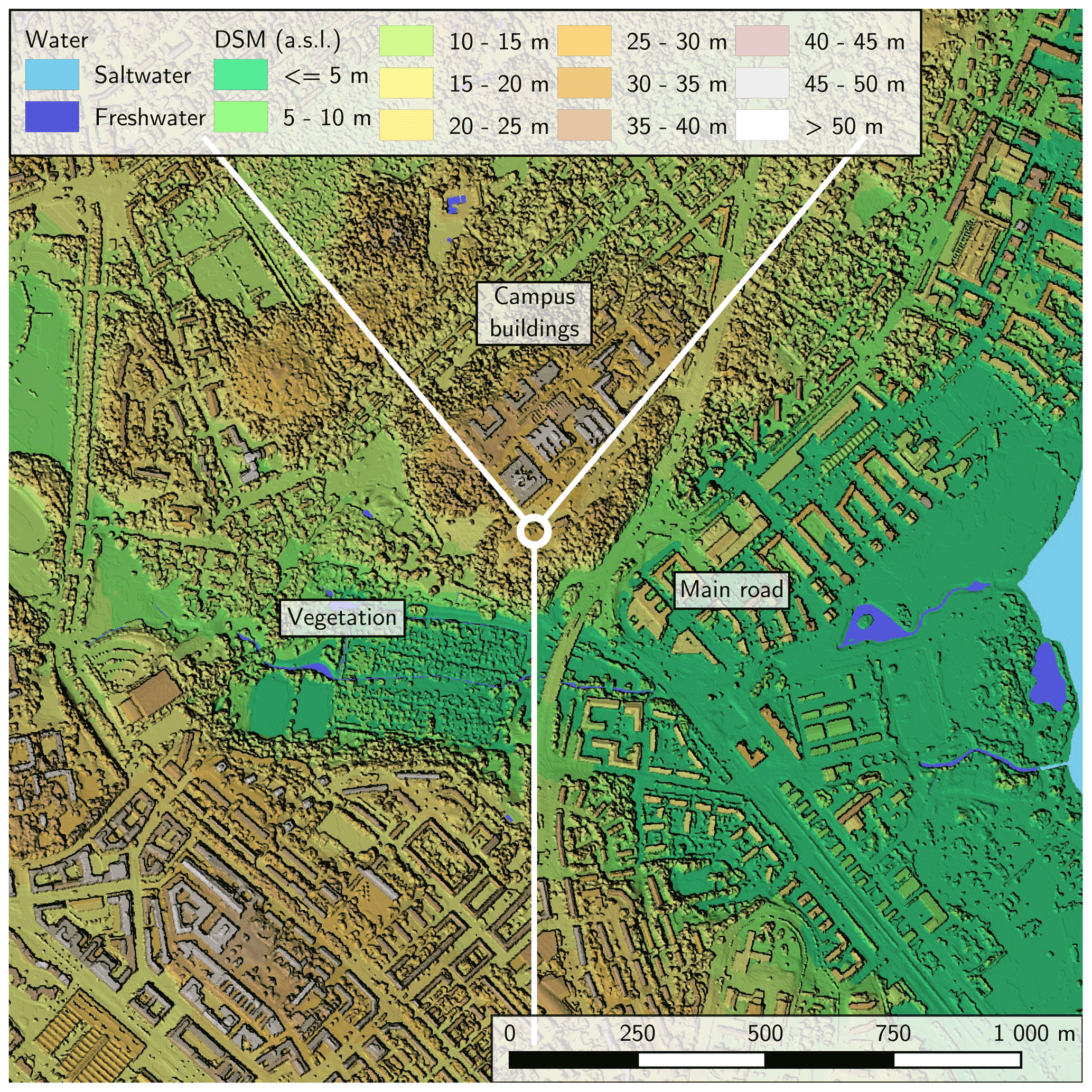
Figure 1 A hill-shaded digital surface model (including vegetation) of the measurement site and surroundings. The mast location is marked with a white circle. Wind sectors defined in Eq. (1) are separated with white lines and labelled. The underlying lidar-derived digital surface model is provided by the City of Helsinki (2017) (CC-BY 4.0).

Overall, the distinctive upwind features around the site can be labelled based on wind direction (WD) as follows (Vesala et al., 2008):

$$\begin{array}{}\text{(1)}& \mathrm{Sector}=\left\{\begin{array}{ll}\mathrm{Campus}\mathrm{buildings},& \mathrm{320}{}^{\circ }\le \mathrm{WD}<\mathrm{40}{}^{\circ },\\ \mathrm{Main}\mathrm{road},& \mathrm{40}{}^{\circ }\le \mathrm{WD}<\mathrm{180}{}^{\circ },\\ \mathrm{Vegetation},& \mathrm{180}{}^{\circ }\le \mathrm{WD}<\mathrm{320}{}^{\circ }.\end{array}\right.\end{array}$$

2.1.2 DTS instrumentation

The DTS system consisted of an optical fibre installed vertically on a 31 m high measurement mast. The measurement instrument (ULTIMA-S, 0–5 km variant; Silixa Ltd, Hertfordshire, UK) was located in an air-conditioned equipment container next to the mast. Fifty-litre cooler tanks were filled with water and used as calibration baths, as in Peltola et al. (2021). One bath was located outside the container and hence the bath water temperature followed the ambient temperature slowly, whereas the other bath was inside the container and the bath water temperature remained at the indoor temperature (around 26 ^∘C). Given the timing of the measurement campaign (winter, early spring), the temperature difference between the baths was adequate for DTS calibration. The water temperatures were monitored with PT100 sensors (supplied and logged with the instrument at 0.01 ^∘C precision) to provide reference temperatures for post-calibration. Both baths were equipped with an aquarium pump to prevent stratification of the water through continuous mixing.

An aramid-reinforced 50 µm multimode fibre-optic cable (AFL Telecommunications LLC, Duncan, SC 29334, USA) was used for the measurements. The total length of the cable was approximately 198 m. A small-diameter white-coated fibre was selected in order to minimise the impact of short-wave radiation exposure, which can potentially have a significant effect on DTS measurements (de Jong et al., 2015). This may be especially important in urban environments, where buildings and other structures can cast hard shadows on the fibre. The fibre was installed to run out of the instrument, through both calibration baths, up and down the mast, again through the calibration baths, and back to the instrument, allowing reference measurements at both the beginning and end of the cable. The fibre, extending from 1.8 to 29 m above ground level (a.g.l.), was attached to the SW side of the mast at five points, with a horizontal separation of approximately 1 m from the mast. Despite careful mounting of the fibre, the connection points caused disturbances in the data, and consequently data points close to the connection points were removed from subsequent analysis. The measurement setup provided a double measurement of the vertical profile of air temperature at 12.7 cm spatial and 1 Hz temporal resolution. In double-ended mode, each direction along the cable was measured sequentially, so that the temperature data at the end were available at 0.5 Hz resolution.

A total of 2202 h of DTS data were recorded over the period of the measurement campaign, covering approximately 90 % of the whole period. The longest measurement break was from 18 March 17:30 UTC to 25 March 12:00 UTC. Three shorter breaks occurred in February: 4 February 13:30 UTC to 6 February 00:00 UTC; 11 February from 01:00 UTC to midnight; and 25 February from 09:00 UTC to midnight. All of these data gaps were due to data transfer issues not related to the instrument itself.

2.1.3 Supporting instrumentation

The measurement mast on which the DTS system was installed features continuous eddy covariance (EC) measurements and auxiliary meteorological measurements. These measurements are part of the ICOS (Integrated Carbon Observation System) research infrastructure. The EC measurement system uses an ultrasonic anemometer (USA-1, Metek GmbH, Germany) to measure 3-D orthogonal wind speed components (u, v, and w) and the sonic temperature (T_s) at a 10 Hz sampling rate. The anemometer is located at the top of the 31 m (60 m a.s.l.) mast.

The data from the anemometer were used in this study as a reference for the DTS-derived temperature statistics as well as for mean wind speed and direction. Measurements from a four-component net radiometer (Huskeflux NR01, Hukseflux Thermal Sensors B.V., the Netherlands) were used to estimate the global radiation exposure. The radiometer is located at the mast top and is sampled at 1 min intervals. Humidity and 2 m temperature observations from a Vaisala HMP 155D (Vaisala Oyj, Finland) probe used at an official weather station located at the site were used, as well as precipitation accumulation measured using an OTT Pluvio2 rain gauge (OTT Hydromet GmbH, Germany).

2.2 Data post-processing

The DTS measurements were post-calibrated using the double-ended calibration method described in detail by de Giesen et al. (2012). First, the raw temperature signal was determined from the ratio of the Stokes and anti-Stokes backscatter using the equation (Farahani and Gogolla, 1999; Hausner et al., 2011)

$$\begin{array}{}\text{(2)}& T(x,t)={\displaystyle \frac{\mathit{\gamma }}{\ln \left(\frac{P_{\mathrm{s}}(x,t)}{P_{\mathrm{as}}(x,t)}\right)+C\left(t\right)+{\int }_{\mathrm{0}}^x\mathit{\delta }\mathit{\alpha }\left(x^{\prime }\right)\mathrm{d}{x}^{\prime }}},\end{array}$$

where T is the post-calibration temperature, γ is a calibration constant, x is the distance from the instrument along the fibre, $P_{\mathrm{s}}(x,t)/P_{\mathrm{as}}(x,t)$ the ratio of the Stokes and anti-Stokes backscatter received at the instrument, C(t) is a time-dependent calibration function, and the last term in the denominator represents the cumulative differential attenuation computed separately for each 30 min averaging period. γ and C(t) were determined in a two-step process described by Peltola et al. (2021): (1) both C(t) and γ were fitted as time-dependent variables, and (2) C(t) was re-fitted while γ was fixed at a constant value equal to the mean of the γ values from the first step. In order to reduce the noise, the two simultaneous T profiles (up and down) were averaged prior to analysis. Furthermore, the potential temperature θ used in the analysis was computed from T by reducing them to the mast base height using the standard dry lapse rate.

Two datasets, one containing 30 min turbulence statistics and one containing de-noised high-frequency data, were computed post-calibration. Thirty-minute turbulence statistics were derived using the methodology described by Lenschow et al. (2000) following Peltola et al. (2021). Prior to estimating the statistics, the DTS data were averaged vertically over 0.5 m distance in order to further reduce the noise. After Reynolds averaging, the fluctuating part of the raw DTS-estimated T signal ($T_{\mathrm{raw}}^{\prime }$) can be written as a combination of the true signal T^′(t) and the time-dependent instrument noise ϵ(t) as $T_{\mathrm{raw}}^{\prime }=T^{\prime }+\mathit{ϵ}$. The second-order autocovariance of the signal can be then written as

$$\begin{array}{}\text{(3)}& M_{\mathrm{11}}\left(t_{\mathrm{1}}\right)=\stackrel{\mathrm{‾}}{\left(T^{\prime }+\mathit{ϵ}\right)\left(T_{\mathrm{1}}^{\prime }+{\mathit{ϵ}}_{\mathrm{1}}\right)},\end{array}$$

where the overline denotes a temporal average and the subscript 1 denotes the lag-t₁ time series. Given that T^′ and ϵ are uncorrelated, it can be shown that

$$\begin{array}{}\text{(4)}& M_{\mathrm{11}}\left(\mathrm{0}\right)=\stackrel{\mathrm{‾}}{{T^{\prime }}^{\mathrm{2}}}+\stackrel{\mathrm{‾}}{{\mathit{ϵ}}^{\mathrm{2}}}.\end{array}$$

Assuming uncorrelated noise, the true signal variance $\stackrel{\mathrm{‾}}{{T^{\prime }}^{\mathrm{2}}}$ and the instrument noise variance $\stackrel{\mathrm{‾}}{{\mathit{ϵ}}^{\mathrm{2}}}$ can be estimated by extrapolating the autocovariance function to lag zero:

$$\begin{array}{}\text{(5)}& {\displaystyle }{\mathit{\sigma }}_T^{\mathrm{2}}=\stackrel{\mathrm{‾}}{{T^{\prime }}^{\mathrm{2}}}=M_{\mathrm{11}}\left(t_{\mathrm{1}}\to \mathrm{0}\right)\text{(6)}& {\displaystyle }\stackrel{\mathrm{‾}}{{\mathit{ϵ}}^{\mathrm{2}}}=M_{\mathrm{11}}\left(\mathrm{0}\right)-M_{\mathrm{11}}\left(t_{\mathrm{1}}\to \mathrm{0}\right).\end{array}$$

For third-order moments, a third-order autocovariance function (M₂₁) can be used similarly:

$$\begin{array}{}\text{(7)}& {\displaystyle }\stackrel{\mathrm{‾}}{{T^{\prime }}^{\mathrm{3}}}=M_{\mathrm{21}}\left(t_{\mathrm{1}}\to \mathrm{0}\right)\text{(8)}& {\displaystyle }\stackrel{\mathrm{‾}}{{\mathit{ϵ}}^{\mathrm{3}}}=M_{\mathrm{21}}\left(\mathrm{0}\right)-M_{\mathrm{21}}\left(t_{\mathrm{1}}\to \mathrm{0}\right).\end{array}$$

The signal-to-noise ratio (SNR) was computed from the second-order statistics:

$$\begin{array}{}\text{(9)}& \mathrm{SNR}={\displaystyle \frac{{\mathit{\sigma }}_T^{\mathrm{2}}}{\stackrel{\mathrm{‾}}{{\mathit{ϵ}}^{\mathrm{2}}}}}.\end{array}$$

To assess the comparability of DTS-estimated higher-order statistics against those estimated from the EC system, the absolute differences between DTS and EC 30 min variance and skewness estimates were computed. For variance, the absolute difference scaled to unit variance, i.e.

$$\begin{array}{}\text{(10)}& D_{{\mathit{\sigma }}_{\mathit{\theta }}^{\mathrm{2}}}={\displaystyle \frac{\left|{\mathit{\sigma }}_{{\mathit{\theta }}_{\mathrm{EC}}}^{\mathrm{2}}-{\mathit{\sigma }}_{{\mathit{\theta }}_{\mathrm{DTS}}}^{\mathrm{2}}\right|}{{\mathit{\sigma }}_{{\mathit{\theta }}_{\mathrm{DTS}}}^{\mathrm{2}}}},\end{array}$$

was used as a difference metric; for skewness, the absolute difference of Pearson's moment coefficients of skewness (S_θ), i.e.

$$\begin{array}{}\text{(11)}& D_{S_{\mathit{\theta }}}=\left|S_{{\mathit{\theta }}_{\mathrm{EC}}}-S_{{\mathit{\theta }}_{\mathrm{DTS}}}\right|,\end{array}$$

was used as a difference metric. The highest measurement height in the post-processed dataset (28.64 m a.g.l.) was used in the comparison. The height separation between the DTS measurement point and the sonic anemometer (31 m a.g.l.) causes a small systematic error in the observed differences between the two measurement methods, but the size of this systematic error was qualitatively assumed to be small enough to be ignored in this study. Furthermore, the root-mean-square difference (RMSD) and 95th percentile range were computed for the deviations for ten equally sized data bins sorted and allocated based on the SNR. These were computed in order to find a level of SNR above which the DTS estimates are reliable enough.

The high-frequency dataset was constructed by de-noising the calibrated raw temperature signal using a singular value decomposition (SVD)-based de-noising methodology similar to that used by Epps and Krivitzky (2019). The SVD of a data matrix $\mathbf{T}\in {\mathrm{\Re }}^{n\times m}$ is

$$\begin{array}{}\text{(12)}& \mathbf{T}=\sum _{i=\mathrm{1}}^n{\mathit{u}}_k{s}_k{\mathit{v}}_k^{\top },\end{array}$$

where u_k is the left singular vector, s_k is a singular value, and v_k is the right singular vector of the kth SVD mode. $s_k^{\mathrm{2}}$ corresponds to the variance of the data matrix at the kth SVD mode and hence the overall variance of the data can be estimated from the sum of all $s_k^{\mathrm{2}}$ values. Following Epps and Krivitzky (2019), it was assumed that at high i, the SVD modes were dominated by noise, and hence s_k at high i follows the Marchenko–Pastur distribution (see Epps and Krivitzky, 2019, for details). Based on this, the clean (i.e. noise-free) singular values (${\stackrel{\mathrm{̃}}{s}}_k$) were reconstructed as

$${\stackrel{\mathrm{̃}}{s}}_k=\left\{\begin{array}{ll}\sqrt{s_k^{\mathrm{2}}-s_{\mathrm{noise},k}^{\mathrm{2}}},& k<k_c\\ \mathrm{0},& k\ge k_c\end{array},\right.$$

where $s_{\mathrm{noise},k}^{\mathrm{2}}$ represents the noise variance at the kth SVD mode, estimated based on the Marchenko–Pastur distribution, and k_c is the minimum index k for which $s_k>s_{\mathrm{noise},k}$. Then the de-noised data matrix $\stackrel{\mathrm{̃}}{\mathbf{T}}$ was reconstructed via

$$\begin{array}{}\text{(13)}& \stackrel{\mathrm{̃}}{\mathbf{T}}=\sum _{i=\mathrm{1}}^n{\mathit{u}}_k{\stackrel{\mathrm{̃}}{s}}_k{\mathit{v}}_k^{\top }.\end{array}$$

Note that this reconstruction was performed using all SVD modes and ${\stackrel{\mathrm{̃}}{s}}_k$, not just the few lowest modes as in Epps and Krivitzky (2019). The de-noising algorithm described above was applied to the temperature profiles using 30 min blocks. The strength of the SVD-based de-noising over de-noising using, for example, wavelets is that SVD is fully data driven, meaning that it is not necessary to find a suitable mother wavelet for the dataset in question.

The turbulent statistics and fluxes were computed from the EC data using commonly accepted procedures following Aubinet et al. (1999), with a data post-processing pipeline used at the site, as described in Nordbo et al. (2013). Flux stationary screening using the 0.3 limit had the most significant effect on EC data availability, reducing the total EC data availability over the measurement period from 2401 to 1559 h.

2.3 Theoretical vertical profiles of potential temperature and its variance in the surface layer

The Monin–Obukhov similarity theory (MOST) can be used to predict 1-D profiles of scaled mean and turbulent quantities within the surface layer. Whilst it is well known that the assumptions used in MOST are not valid in the RSL (Rotach, 1999; Barlow, 2014), which can cover a large portion of the surface layer of the UBL, it is nevertheless a widely used theoretical reference for lower boundary layer profile studies. MOST predicts that the mean and turbulence profiles can be parametrised as unique functions of the stability parameter (Monin and Obukhov, 1954):

$$\begin{array}{}\text{(14)}& \mathit{\zeta }=z/L,\end{array}$$

where z is the effective measurement height (the measurement height reduced by the possible displacement height) and L is the Obukhov length, defined as

$$\begin{array}{}\text{(15)}& L={\displaystyle \frac{-u_{*}^{\mathrm{3}}\stackrel{\mathrm{‾}}{\mathit{\theta }}}{kg\stackrel{\mathrm{‾}}{w^{\prime }{\mathit{\theta }}^{\prime }}}},\end{array}$$

where u_* is the friction velocity, $\stackrel{\mathrm{‾}}{\mathit{\theta }}$ is the mean potential temperature, k is von Kármán's constant, g is the gravitational acceleration, and $\stackrel{\mathrm{‾}}{w^{\prime }{\mathit{\theta }}^{\prime }}$ is the kinematic heat flux.

Using the surface layer temperature scale

$$\begin{array}{}\text{(16)}& {\mathit{\theta }}_{*}=-{\displaystyle \frac{\stackrel{\mathrm{‾}}{w^{\prime }{\mathit{\theta }}^{\prime }}}{u_{*}}},\end{array}$$

the surface layer temperature gradient can be parametrised as a function of ζ:

$$\begin{array}{}\text{(17)}& {\displaystyle \frac{\partial \stackrel{\mathrm{‾}}{\mathit{\theta }}}{\partial z}}={\displaystyle \frac{{\mathit{\theta }}_{*}}{kz}}{\mathit{\varphi }}_{\mathit{\theta }}\left(\mathit{\zeta }\right),\end{array}$$

where ϕ_θ is a similarity function for mean temperature. The temperature profile in the surface layer can then be obtained by integration:

$$\begin{array}{}\text{(18)}& \stackrel{\mathrm{‾}}{\mathit{\theta }}\left(z_{\mathrm{2}}\right)-\stackrel{\mathrm{‾}}{\mathit{\theta }}\left(z_{\mathrm{1}}\right)={\displaystyle \frac{{\mathit{\theta }}_{*}}{k}}\underset{z_{\mathrm{1}}}{\overset{z_{\mathrm{2}}}{\int }}{\displaystyle \frac{\mathrm{1}}{z}}{\mathit{\varphi }}_{\mathit{\theta }}\left(\mathit{\zeta }\right)\partial z.\end{array}$$

Various forms of ϕ_θ have been proposed over the years, with the so-called Businger–Dyer form (Businger, 1988)

$$\begin{array}{}\text{(19)}& \begin{array}{rl}& {\mathit{\varphi }}_{\mathit{\theta }}\left(\mathit{\zeta }\right)=\mathrm{1}+C_{\mathrm{1}}\mathit{\zeta },\mathrm{when}\mathit{\zeta }>\mathrm{0}\\ & {\mathit{\varphi }}_{\mathit{\theta }}\left(\mathit{\zeta }\right)=(\mathrm{1}-C_{\mathrm{2}}\mathit{\zeta }{)}^{-\mathrm{1}/\mathrm{2}},\mathrm{when}\mathit{\zeta }<\mathrm{0}\end{array},\end{array}$$

where the constants C₁ and C₂ are determined empirically, being one of the most commonly used.

Instead of the detailed temperature profile described by Eq. (18), it is often enough and useful to describe the overall stratification within an air column between z₁ and z₂ using a single measure. For this, the column-integrated buoyancy B (Lareau and Horel, 2015), where

$$\begin{array}{}\text{(20)}& B=g\underset{z_{\mathrm{1}}}{\overset{z_{\mathrm{2}}}{\int }}\left[{\displaystyle \frac{{\mathit{\theta }}_{z_{\mathrm{1}}}-{\mathit{\theta }}_{z_{\mathrm{2}}}}{{\mathit{\theta }}_{z_{\mathrm{1}}}}}\right]\partial z\end{array}$$

can be used. As the name suggests, this represents the integrated buoyant force across the defined column. The MOST-predicted B can be estimated and subsequently compared to the observed B by further integrating Eq. (18) as above.

Similarly to mean quantities, the integral turbulence characteristics (ITCs), i.e. the standard deviations of turbulent variables normalised using their respective scaling, can be parametrised using MOST. Using the surface layer temperature scale θ_*, we can write the parametrisation for the standard deviation of potential temperature as (Panofsky et al., 1977)

$$\begin{array}{}\text{(21)}& {\displaystyle \frac{{\mathit{\sigma }}_{\mathit{\theta }}}{{\mathit{\theta }}_{*}}}={\mathit{\varphi }}_{{\mathit{\sigma }}_{\mathit{\theta }}}\left(\mathit{\zeta }\right),\end{array}$$

where ${\mathit{\varphi }}_{{\mathit{\sigma }}_{\mathit{\theta }}}$ is a similarity function for the temperature ITC. A widely suggested form for ${\mathit{\varphi }}_{{\mathit{\sigma }}_{\mathit{\theta }}}$ in unstable conditions is (e.g. Panofsky et al., 1977; Kaimal and Finnigan, 1994; Liu et al., 1998; Andreas et al., 1998; Wilson, 2008)

$$\begin{array}{}\text{(22)}& {\mathit{\varphi }}_{{\mathit{\sigma }}_{\mathit{\theta }}}\left(\mathit{\zeta }\right)=C_{\mathrm{1}}{\left(\mathrm{1}-C_{\mathrm{2}}\mathit{\zeta }\right)}^{C_{\mathrm{3}}},\end{array}$$

where the constants C₁, C₂, and C₃ are determined empirically. A recent large eddy-simulation-based study by Maronga and Reuder (2017) found values of $C_{\mathrm{1}}=-\mathrm{2.1}$ and C₂=9 for $C_{\mathrm{3}}=-\mathrm{1}/\mathrm{3}$, which is the power traditionally used in the literature. These values produce similar results to the sonic-anemometer-measurement-based studies by Andreas et al. (1998) and Liu et al. (1998), who found values of ($C_{\mathrm{1}}=-\mathrm{2.0}$, C₂=8) and ($C_{\mathrm{1}}=-\mathrm{3.2}$, C₂=28.4), respectively. Maronga and Reuder (2017) also suggested a slightly different shape for the similarity function, with $C_{\mathrm{3}}=-\mathrm{0.4}$ based on the simulation data, but due to the lack of measurement-based evidence, we used the values for the traditional $C_{\mathrm{3}}=-\mathrm{1}/\mathrm{3}$ form suggested by the study.

Assuming the validity of MOST and vertically constant fluxes, θ_* and L are expected to be near constant in the surface layer, and Eqs. (21) and (22) can be used to predict the profiles of $\stackrel{\mathrm{‾}}{\mathit{\theta }}$ and σ_θ, respectively, using EC measurements from only one level. In reality, the presence of a constant flux layer depends on how developed the flow is, which itself depends on upwind surface heterogeneities and large-scale atmospheric forcing (e.g. Rotach, 1999). Additionally, closer to the ground, namely in the roughness sublayer, local heterogeneity of the flow breaks the assumptions of a constant flux layer and subsequently those of MOST. Thus, observed profiles of ITCs are expected to deviate from those predicted using MOST in the lower portions of the surface layer.

2.4 Wavelet analysis

To study the spectro-temporal properties of the measured time series, we utilise the continuous wavelet transform (CWT). In CWT, as for wavelet transforms (WT) in general, a wavelet function is used to unfold a signal into time-frequency space.

The CWT of a finite discrete signal of a turbulent quantity q(t_m) with a uniform time step δt is obtained by convolving it with a scaled and translated analysing wavelet Ψ(η_m). After normalisation to unit energy, this can be written as

$$\begin{array}{}\text{(23)}& W_q(s,t_n)={\left({\displaystyle \frac{\mathit{\delta }t}{s}}\right)}^{\mathrm{1}/\mathrm{2}}\sum _{m=\mathrm{0}}^{N}q\left(t_m\right){\mathrm{\Psi }}_{\mathrm{0}}^{*}\left({\mathit{\eta }}_m\right)\mathit{\delta }t,\end{array}$$

where ${\mathit{\eta }}_m=\left(t_m-t_n\right)/s$, ${\mathrm{\Psi }}_{\mathrm{0}}^{*}\left({\mathit{\eta }}_m\right)$ is the complex conjugate of Ψ(η_m) normalised to unit energy and ${\left(\mathit{\delta }t/s\right)}^{\mathrm{1}/\mathrm{2}}$ is a scaling factor. By altering the wavelet scale s and translating along the localised time index t_n, one can evaluate the function W_q(s, t_n) on a timescale plane, producing a scalogram. The finite bounds used in Eq. (23) induce significant edge effects when the wavelet's cone of influence, i.e. e-folding time of Ψ(η_m), extends beyond the bounds of the original time series (Torrence and Compo, 1998).

Although the selection of scales to be used for CWT can theoretically be arbitrary, for reconstruction purposes it is convenient to construct the scales as fractional powers of 2 (Torrence and Compo, 1998):

$$\begin{array}{}\text{(24)}& s_j=s_{\mathrm{0}}{\mathrm{2}}^{j\mathit{\delta }j},\mathrm{for}j=\mathrm{0},\mathrm{1},\mathrm{\dots },J,\end{array}$$

where s₀ is the smallest resolvable scale, δj is the spacing factor, and J is the number of scales plus one. To include scales up to the largest scale possible given the length of the time series, one can select $J={\mathit{\delta }}_j^{-\mathrm{1}}{\log }_{\mathrm{2}}\left(N\mathit{\delta }t/s_{\mathrm{0}}\right)$.

Following the bias rectification proposed by Liu et al. (2007), the discrete wavelet power of the signal can be computed from the normalised transform as the square of the norm of the transform divided by the associated scale: ${\left|W_q(s_j,t_n)\right|}^{\mathrm{2}}/s_j$. From this, the global discrete wavelet variance spectrum can be reconstructed as

$$\begin{array}{}\text{(25)}& E_q\left(s_j\right)={\displaystyle \frac{\mathit{\delta }j\mathit{\delta }t}{C_{\mathit{\delta }}}}{\displaystyle \frac{\mathrm{1}}{N}}\sum _{n=\mathrm{0}}^N{\displaystyle \frac{{\left|W_q(s_j,t_n)\right|}^{\mathrm{2}}}{s_j}},\end{array}$$

where C_δ is a wavelet-specific reconstruction factor. E_q is defined here in such a way that an estimate of the global variance of the time series can be reconstructed as the sum of E_q(s_j) over all s_j defined in Eq. (24),

$$\begin{array}{}\text{(26)}& {\mathit{\sigma }}_q^{\mathrm{2}}=\sum _{j=\mathrm{0}}^J{E}_q\left(s_j\right),\end{array}$$

analogous to the Fourier discrete variance spectrum described in Stull (1988). The accuracy of this variance estimate depends on the spacing factor δj used and the analysing wavelet (Schaller et al., 2017). Similarly, a local variance estimate can be reconstructed as

$$\begin{array}{}\text{(27)}& {\mathit{\sigma }}_q^{\mathrm{2}}\left(t_n\right)={\displaystyle \frac{\mathit{\delta }j\mathit{\delta }t}{C_{\mathit{\delta }}}}\sum _{j=\mathrm{0}}^J{\displaystyle \frac{{\left|W_q(s_j,t_n)\right|}^{\mathrm{2}}}{s_j}},\end{array}$$

producing a temporally localised variance estimate with a time resolution of δt. Although localised in time, this estimate includes variance contributions from all scales represented by s_j, and is thus well suited to studying non-stationary conditions and short-time events, as no steady-state assumption is required (Schaller et al., 2017). By limiting the s_j range included in the sum, band-passed localised variance estimates can be obtained.

The selection of a wavelet depends on multiple factors, which are discussed in detail for example in Farge (1992) and Torrence and Compo (1998). For our case, we selected the Morlet wavelet, a non-orthogonal complex wavelet which provides a good relative balance between time and frequency localisation (e.g. Baars et al., 2015). Formally, the Morlet wavelet is a complex-valued plane wave carrier in a Gaussian envelope (Farge, 1992)

$$\begin{array}{}\text{(28)}& {\mathrm{\Psi }}_{\mathrm{0}}\left(\mathit{\eta }\right)={\mathit{\pi }}^{-\mathrm{1}/\mathrm{4}}{e}^{i{\mathit{\omega }}_{\mathrm{0}}\mathit{\eta }}{e}^{-{\mathit{\eta }}^{\mathrm{2}}/\mathrm{2}},\end{array}$$

where ω₀ is a non-dimensional frequency and the subscript zero in Ψ₀ indicates that the wavelet is normalised to unit energy. By varying ω₀, the relative balance between time and scale localisation can be altered. A value of ω₀=6 is commonly used. For the Morlet wavelet, the equivalent Fourier wavelength λ of a given wavelet scale can be computed from the relation (Torrence and Compo, 1998)

$$\begin{array}{}\text{(29)}& \mathit{\lambda }={\displaystyle \frac{\mathrm{4}\mathit{\pi }s}{{\mathit{\omega }}_{\mathrm{0}}+\sqrt{\mathrm{2}+{\mathit{\omega }}_{\mathrm{0}}^{\mathrm{2}}}}}.\end{array}$$

Subsequently, the spectral energy density can be estimated with the help of Eq. (25) as

$$\begin{array}{}\text{(30)}& S_q={\displaystyle \frac{E_q\left(s_j\right)}{\mathrm{\Delta }f\left(s_j\right)}},\end{array}$$

where f(s_j) is the Fourier frequency corresponding to s_j.

3 Results and discussion

3.1 Data quality and conditional sampling

To evaluate the influence of short-wave radiation exposure on the fibre, deviations of the DTS-estimated 30 min 2 m average potential temperature ${\stackrel{\mathrm{‾}}{\mathit{\theta }}}_{\mathrm{DTS}}$ from the 2 m reference temperature were studied as a function of the mean global radiation $\stackrel{\mathrm{‾}}{Q}$ (Fig. 2a). On average, the deviations show a near-zero dependency on $\stackrel{\mathrm{‾}}{Q}$, with a least-squares linear fit slope of ${\mathit{\beta }}_{\mathrm{1}}=\mathrm{6.4}\times {\mathrm{10}}^{-\mathrm{5}}$ K W⁻¹ m²​​​​​​​. The overall root-mean-square error (RMSE) for ${\stackrel{\mathrm{‾}}{\mathit{\theta }}}_{\mathrm{DTS}}$ is 0.23 K, 23 times the reported temperature resolution of the DTS sensor (0.01 K). The radiation-induced error is significantly smaller than reported for a white fibre by de Jong et al. (2015) (0.61 K), potentially due to the smaller outer diameter of the fibre used (0.9 mm vs. 1.6 mm here). Moreover, de Jong et al. (2015) had their cables aligned horizontally, whereas in our measurement setup the cables were aligned with the vertical, which should result in less radiation per unit of cable surface. As the fibre is unprotected from precipitation, evaporative cooling of the precipitation-wetted fibre causes the DTS system to measure the wet bulb temperature instead of the air temperature. This is highlighted in Fig. 2b: the 30 min periods with accumulated liquid-phase precipitation of P≥0.1 mm show a negative bias compared to the reference, whereas the remaining data do not show such a bias. This is expected, as the wet bulb temperature is always less than or equal to the air temperature, and the two are only equal in water-vapour-saturated air. It also explains the relatively high number of data points with negative deviations close to $\stackrel{\mathrm{‾}}{Q}=\mathrm{0}$ W m⁻² in Fig. 2a. This highlights the usefulness of accompanying DTS measurements with precipitation and humidity measurements, and the importance of knowing the meteorological conditions when analysing DTS measurements. The remaining deviations not explained by precipitation or short-wave exposure may arise from multiple sources, including the horizontal separation of the sensors and long-wave radiative cooling of the cable at night.

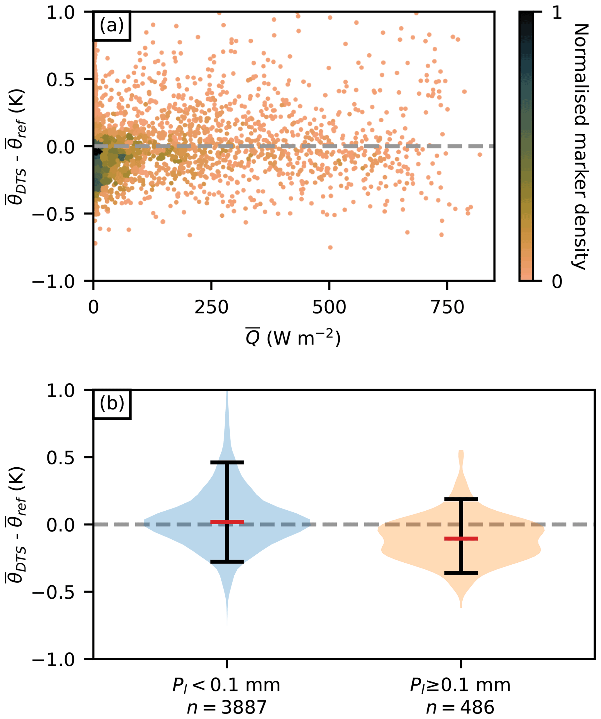
Figure 2 (a) Deviations of the DTS-estimated 30 min potential temperature (${\stackrel{\mathrm{‾}}{\mathit{\theta }}}_{\mathrm{DTS}}$) from the corresponding mean reference potential temperature (${\stackrel{\mathrm{‾}}{\mathit{\theta }}}_{\mathrm{ref}}$) measured at an official weather station next to the measurement mast as a function of global radiation $\stackrel{\mathrm{‾}}{Q}$. The colour scale illustrates the relative marker density. (b) A violin plot of the same deviations for two groups of data: 30 min accumulated liquid-phase precipitation P_l<0.1 mm and P_l≥0.1 mm. Violin bodies represent the data distributions, black whiskers show the 5th to 95th interpercentile ranges, and the red lines show the medians.

Comparisons of the DTS-estimated higher-order statistics against those estimated from the EC system (Fig. 3) reveal a divergence in estimates between the two measurement techniques as the SNR approaches zero. This is caused by two factors. The accuracy of the statistics estimation using the Lenschow method decreases with the SNR and therefore some conditional sampling based on the SNR is required in order to improve the reliability of the estimates. For variance estimates, the RMSD does not decrease with SNR past the fifth data bin, centred at SNR=0.26, with the 95th percentile difference converging at the sixth data bin, centred at SNR=0.37. However, the skewness RMSD decreases up to the seventh bin, centred at SNR=0.55, with the 95th percentile difference decreasing even up to the eighth bin. Determining a minimum acceptable level of SNR for which the estimation of turbulent quantities is still reasonable requires a subjective interpretation. We chose SNR=0.5 as a conservative threshold value, based on both the variance and skewness RMSD curves. The same threshold value was used by Peltola et al. (2021).

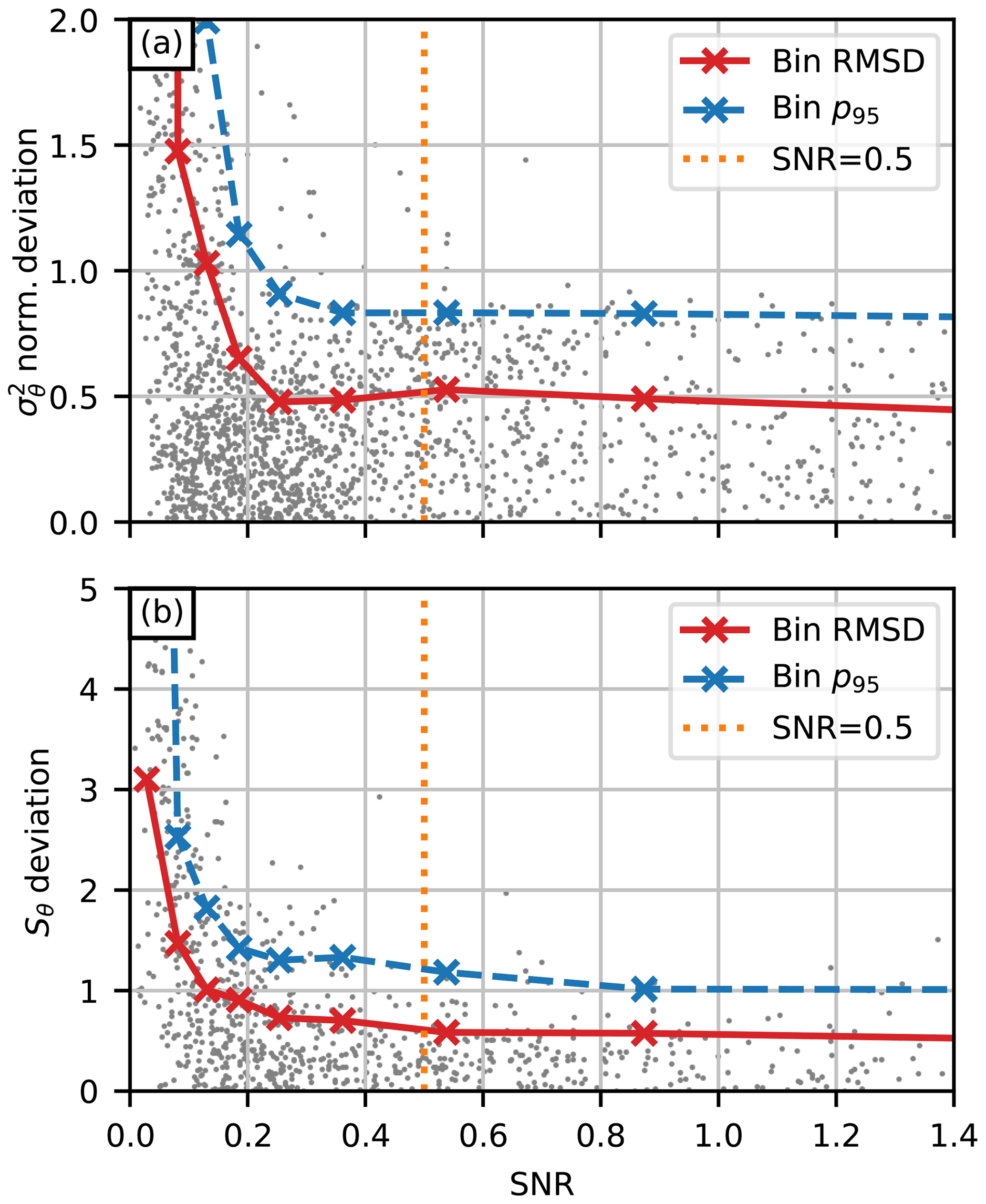
Figure 3 Deviations of the DTS-estimated temperature (a) variance and (b) skewness from the corresponding estimates using the sonic anemometer data. The solid red lines are the root-mean-square-deviations (RMSD) computed for 10 equally sized bins (bin centres are marked with × symbols). The dashed blue lines are the corresponding 95th percentiles for each bin.

As the magnitude of the signal noise is nearly constant, SNR-based screening of the 30 min averaged dataset effectively results in conditional sampling biased towards conditions with higher temperature variance. Temperature fluctuations are generally produced by either thermal turbulence in unstable conditions or mechanically induced turbulent mixing of a stably stratified temperature profile, bringing gusts of warmer air aloft downwards. Neither of these are strong; they have low absolute values of ζ, corresponding to neutral or near-neutral conditions. Therefore, a significant portion of the data corresponding to these conditions are removed in SNR-based screening. This is clearly visible in the frequency distributions of EC-derived ζ after screening, as illustrated in Fig. 4. The ζ distribution corresponding to the filtered dataset is heavily biased towards unstable conditions. However, some of the 30 min averaging periods with more stable conditions are retained, likely due to mechanically induced​​​​​​​ mixing across a stably stratified profile, causing temperature fluctuations.

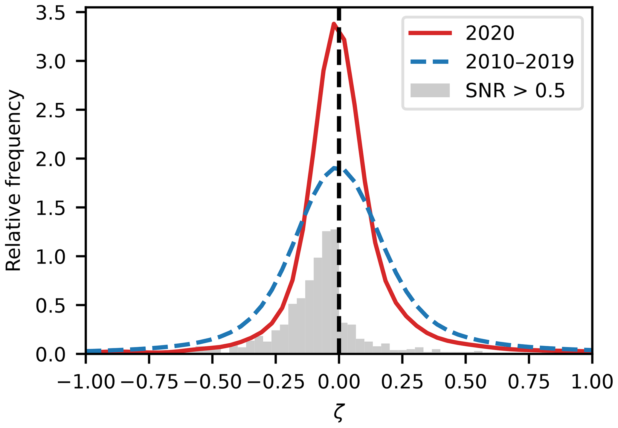
Figure 4 Relative frequency distribution of the EC-derived 30 min stability parameter ζ for the DTS measurement period (solid red line), the same after conditional sampling with SNR>0.5 (grey bars), and the same for the 10-year reference period including only the days of year within the DTS measurement period (dashed blue line). The continuous distributions were estimated from the EC data using kernel density estimation with a Gaussian kernel.

In general, the measurement period in 2020 was less variable stability-wise than a 10-year reference period computed over the same days of year as for the DTS measurement period. With few clear-sky days with strong temperature inversions, near-neutral conditions prevailed, producing a more concentrated ζ distribution around zero compared to the reference period. As a consequence, screening with SNR=0.5 results in only 42 % of the 30 min averaging periods being retained. Had the weather been more typical of the period, this percentage would probably have been higher, as there would have been more averaging periods with higher |ζ|. The resulting bias towards higher |ζ| emphasises the relatively high sensitivity of the DTS system performance to meteorological conditions, which is important to keep in mind when planning DTS measurements.

When studying the portion of data retained as a function of height and time (Fig. 5), the role of solar radiation in the generation of temperature fluctuations becomes evident. More data are retained in late spring, around midday, and closer to the ground, when/where the occurrence of acceptable SNR values reaches 60 %–80 %. According to MOST, the temperature variance increases with decreasing height within the surface layer (Eq. 21), which in turn may cause the SNR to cross the threshold value mid-profile in certain conditions. As expected, SNR shows a clear nocturnal cycle and an increasing trend over the whole measurement period. This emphasises that SNR-screened DTS-estimated statistics are not equally representative of all times of day and days of year.

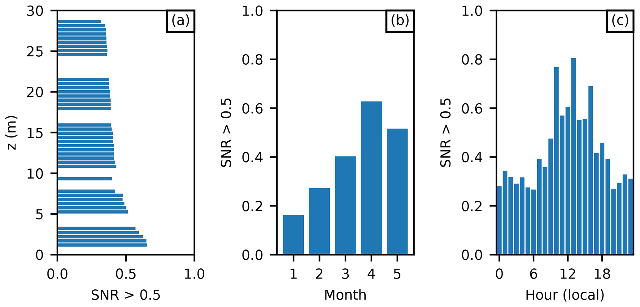
Figure 5 Fraction of the data preserved (i.e. that fulfil the SNR>0.5 threshold) as functions of (a) the height, (b) the month, and (c) the hour of day in local time (EET/EEST). Note that January and May only contain data from 5 d.

3.2 Surface layer scaling

One of the main benefits of DTS is the potential for larger spatial coverage than with conventional techniques, such as sonic anemometers. In Fig. 6, the profiles of DTS-derived temperature ITCs for unstable conditions are compared to predictions from the similarity function in Eq. (22) and to those estimated from the EC measurements. The similarity functions converge to similar values in DTS and EC at the top of the mast, and are generally in good agreement with the DTS throughout the profile for very unstable conditions ($\mathit{\zeta }<-\mathrm{0.3}$). For mildly unstable conditions ($-\mathrm{0.3}>\mathit{\zeta }>-\mathrm{0.05}$), there is a discrepancy between the profiles that grows considerably on moving down the profile towards the surface. This is not unexpected, since the lowest measurement levels are in the roughness sublayer in all wind directions, where MOST scaling is not expected to hold. For the main road wind sector especially, the deviation of the DTS profile from the similarity function is already considerable quite far up the profile. It is possible that the deviation is caused by upstream inhomogeneities in the surface properties. Given that the sea is approximately 1–2 km away in the direction of the main road, in mildly unstable conditions there may be, at least occasionally, a thermal IBL with a height less than the mast top height. This would result in the observed median temperature ITC profile, which drastically exceeds that predicted by the MOST similarity relation for the lower sections of the mast.

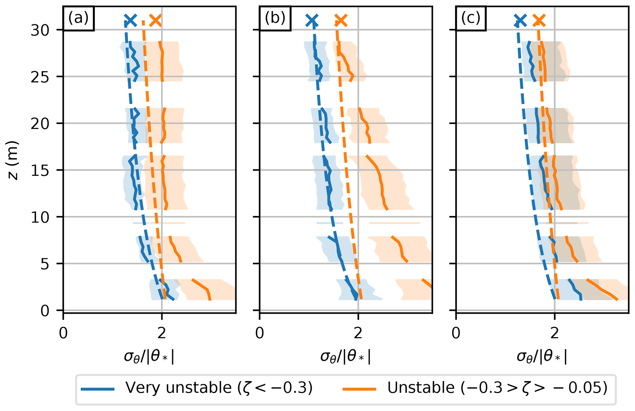
Figure 6 Median profiles of normalised temperature standard deviations (ITCs) in unstable conditions (solid lines) for three wind sectors: (a) campus buildings, (b) main road, and (c) vegetation, with the p_25–75 interpercentile range shaded. The corresponding estimates from the EC system are marked with × symbols, and reference similarity functions are drawn using dashed lines.

It should be emphasised that the zero-plane displacement height was ignored when computing the similarity functions assuming minimal local displacement of the wind profile. As the mast is located on a hill top and the measurements were performed during the leaf-free season, it is challenging to prove the existence of a well-defined zero-plane displacement. The DTS-estimated profiles do not show any clear discontinuity in shape. With a taller measurement mast, the DTS profiles could be used to obtain the displacement height by fitting a similarity function to the data with displacement height as the sole regressor. This could only be done if a significant stretch of the fibre was located clearly above the roughness sublayer; the current measurement mast is too short.

3.3 Warm front on 27 January 2020

Although many averaged DTS data points have been filtered out by the SNR criteria, the high-frequency data can still be used to study meteorological phenomena. To demonstrate the possibilities of using DTS data in low-SNR conditions, we studied measurements made during a passage of a warm front in closer detail. Late in the evening of 27 January 2020, a warm front associated with a North Atlantic low-pressure system passed over Southern Finland and Helsinki, eroding the near-ground cold layer beneath by downward mixing of the warm air aloft. Figure 7 presents the near-surface wind and temperature observations from nearby weather stations at the time the surface front reached the measurement site (21:30 UTC, 23:30 local time). The west–north-west to east–south-east alignment of the front is visible as a strong surface temperature gradient and a turning of the winds from SE to SW. Due to the inherently stable conditions and low wind speeds (1.7 to 3.3 m s⁻¹) during the passage of the front, the average SNR value was only 0.13 during this approximately 1 h event, significantly less than the SNR=0.5 threshold used in the quality screening for the 30 min averaged datasets. Furthermore, the nature of the event caused EC data to also be flagged during flux stationarity screening, emphasising the non-stationary nature of the event. From 16:00 to 23:20 UTC, 100 % relative humidity was constantly observed at the official weather station, indicating very humid conditions.

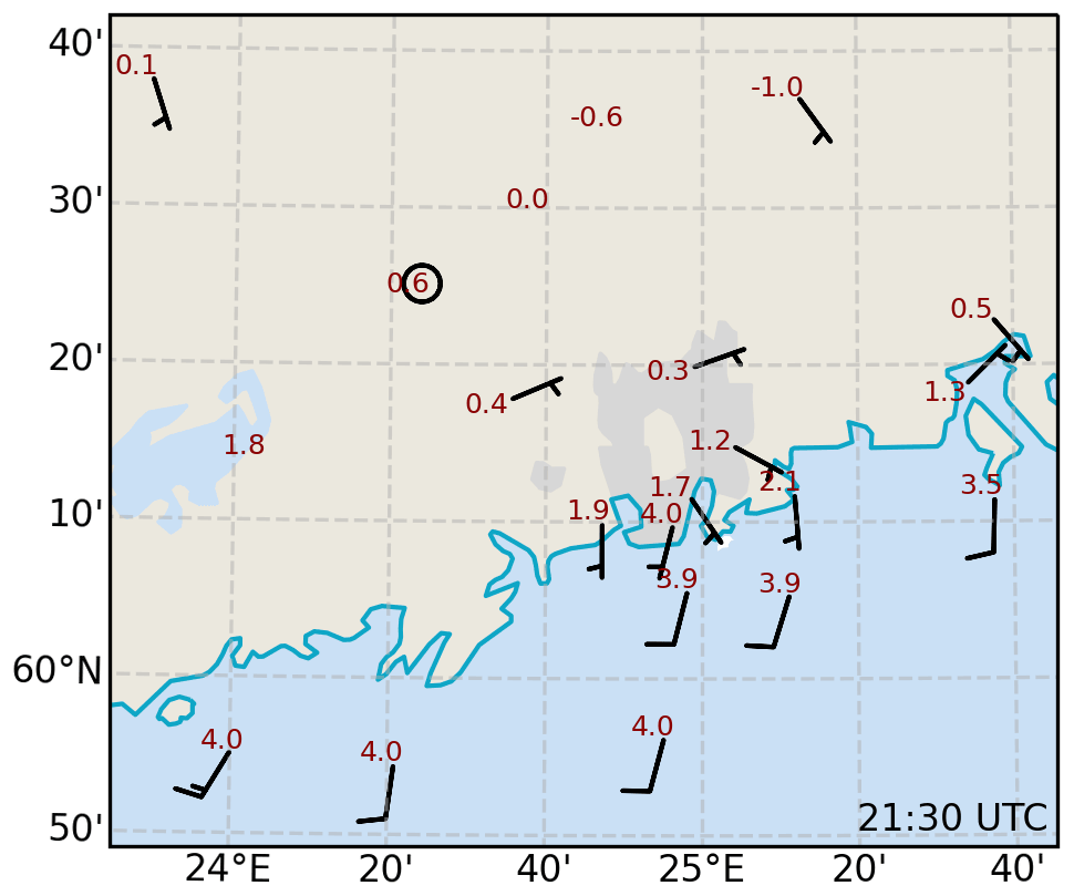
Figure 7 Surface observations of temperature and wind from official weather stations close to Helsinki on 27 January 2020 at 21:30 UTC.

Plotting the DTS-observed high-frequency $\stackrel{\mathrm{̃}}{\mathit{\theta }}$ time series (Fig. 8a) reveals a turbulently progressing mixing process during the front passage. Warmer air aloft is mechanically entrained relatively slowly downwards, progressively increasing the temperatures along the profile. Time series of the column-integrated buoyancy (B) along the DTS profile (Fig. 8b) provide a more comprehensive overall picture of the thermal structure and propagation of the front. The average B starts to decrease from near neutral at approximately 20:50 UTC, reaching −0.57 m² s⁻², and returns to near neutral at 22:10 UTC. This demonstrates how, with the lack of thermal turbulence production in the stably stratified boundary layer, turbulence is generated through shear instability, which allows warmer air aloft to be entrained during the passage of the front. Inspecting the high-frequency B time series reveals considerable deviations from the 10 min moving average, with peaks up to −1.1 m² s⁻². These deviations are of the same order as the mean value, and one deviation causes the profile stability to return back to neutral briefly at 21:51 UTC.

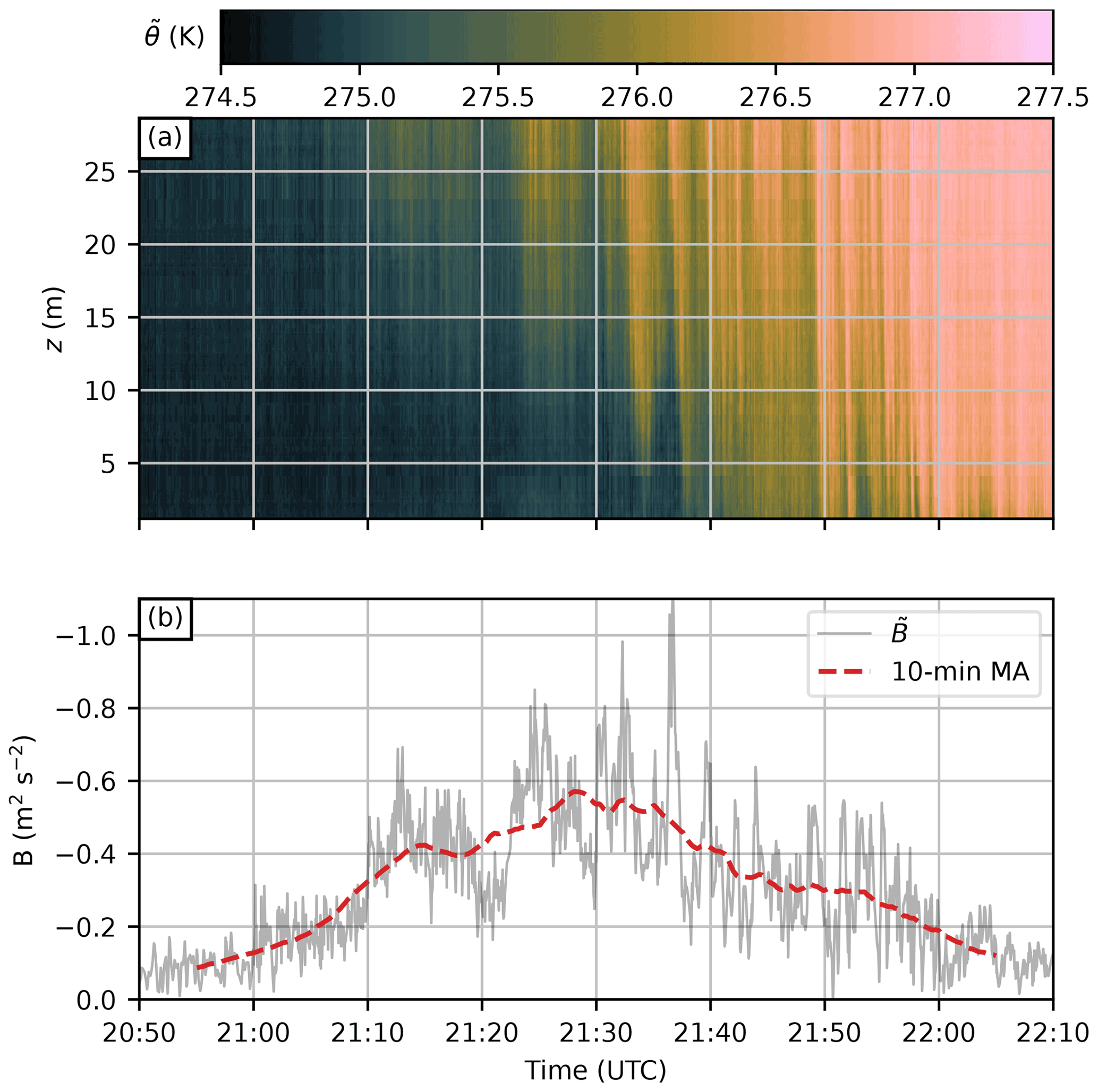
Figure 8 (a) De-noised high-frequency potential temperature ($\stackrel{\mathrm{̃}}{\mathit{\theta }}$) time series for the event on 27 January 2020. Linear interpolation was used to interpolate the data gaps along the fibre caused by fibre attachment point interference. (b) Column-integrated buoyancy (solid grey line) over the DTS profile and the respective 10 min moving average (dashed red line).

By plotting the $\stackrel{\mathrm{̃}}{\mathit{\theta }}$ over the event at individual heights, it was empirically determined that a logistic function of the form

$$\begin{array}{}\text{(31)}& \stackrel{\mathrm{̃}}{\mathit{\theta }}\left(t\right)={\displaystyle \frac{\mathrm{\Delta }\mathit{\theta }}{\mathrm{1}+\exp \left(-k\left(t-t_{\mathrm{0}}\right)\right)}},\end{array}$$

where Δθ is the difference in θ before and after the event, k is the rate parameter, and t₀ is the temporal midpoint parameter, describes the general temporal evolution of $\stackrel{\mathrm{̃}}{\mathit{\theta }}$ over the event reasonably well (as demonstrated for two heights in Fig. 9a). Using this logistic regression to describe the $\stackrel{\mathrm{̃}}{\mathit{\theta }}$ evolution is particularly useful in this case, as it permits the analysis of the downward propagation of the inversion layer using t₀ and the gradient of $\stackrel{\mathrm{̃}}{\mathit{\theta }}$ in time using k. The rate parameter k increases as the inversion propagates downwards until z≈6 m, from where it starts to decrease towards the ground. The inversion layer can be estimated to propagate downwards at an average rate of $\mathrm{2.5}\times {\mathrm{10}}^{-\mathrm{2}}$ m s⁻¹ when determined from the t₀ profile (Fig. 9c), i.e., on average, the temperature curve lags 40 s behind the one measured from 1 m above. This rate is relatively constant throughout the profile.

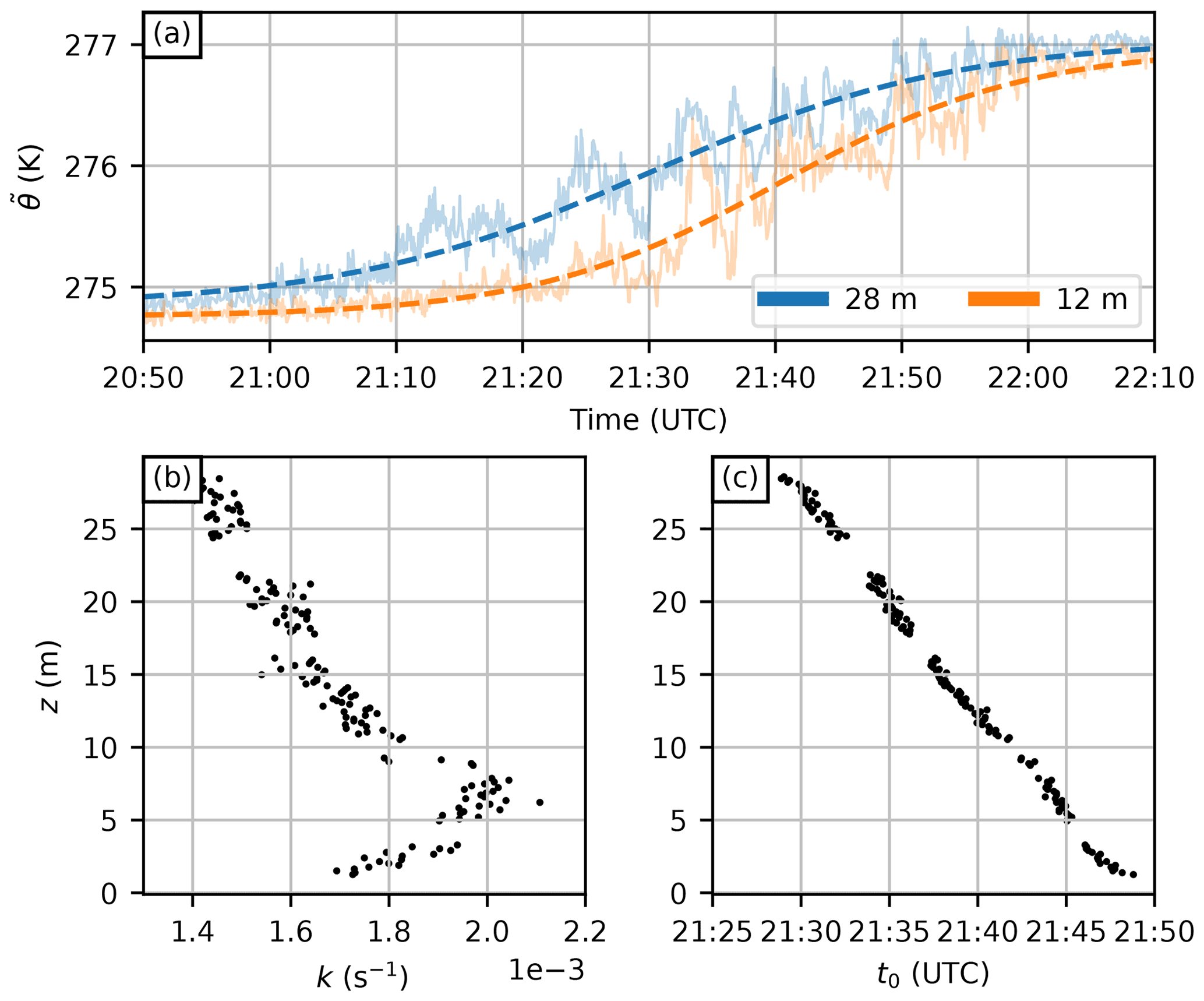
Figure 9 (a) Time series of $\stackrel{\mathrm{̃}}{\mathit{\theta }}$ from two heights (solid lines) and the corresponding logistic regression curve (dashed lines) for the event on 27 January 2020. (b) The rate parameter (k) of a logistic regression on $\stackrel{\mathrm{̃}}{\mathit{\theta }}$ as a function of height. (c) Same as (b) but for the temporal midpoint parameter (t₀) of the function.

To study the turbulence behaviour in detail during the passage, wavelet transforms of $\stackrel{\mathrm{̃}}{\mathit{\theta }}$ at two heights (28 and 12 m) were computed, along with wavelet transforms of T_s measured by the sonic anemometer and the noise signal $\mathit{\theta }-\stackrel{\mathrm{̃}}{\mathit{\theta }}=\mathit{ϵ}$ from the respective heights for reference. The resulting wavelet-derived spectral energy density (Fig. 10a) reveals that, during the event, the vast majority of the DTS signal for $f>{\mathrm{10}}^{-\mathrm{2}}$ Hz is noise. However, the spectral peaks in the EC-derived energy density support our assertion that the dominant scales in the event lie at frequencies below $f={\mathrm{10}}^{-\mathrm{2}}$ Hz. The EC and DTS (28 m) spectra compare relatively well, with the major difference being a peak missing from the DTS spectrum at around $f=\mathrm{8}\times {\mathrm{10}}^{-\mathrm{4}}$ Hz (corresponding roughly to a 21 min timescale). The underestimation of the variance at this scale might be caused by the fact that the de-noising algorithm was applied with a 30 min time step and hence the underestimation is not directly related to the instrument. Within the frequency band $\mathrm{6.2}\times {\mathrm{10}}^{-\mathrm{4}}$ Hz < f < $\mathrm{1.0}\times {\mathrm{10}}^{-\mathrm{2}}$ Hz, which contains 84 % of the total temperature variance according to the EC data, the average SNR at the two heights is 3.3, a number much higher than that for the whole spectrum.

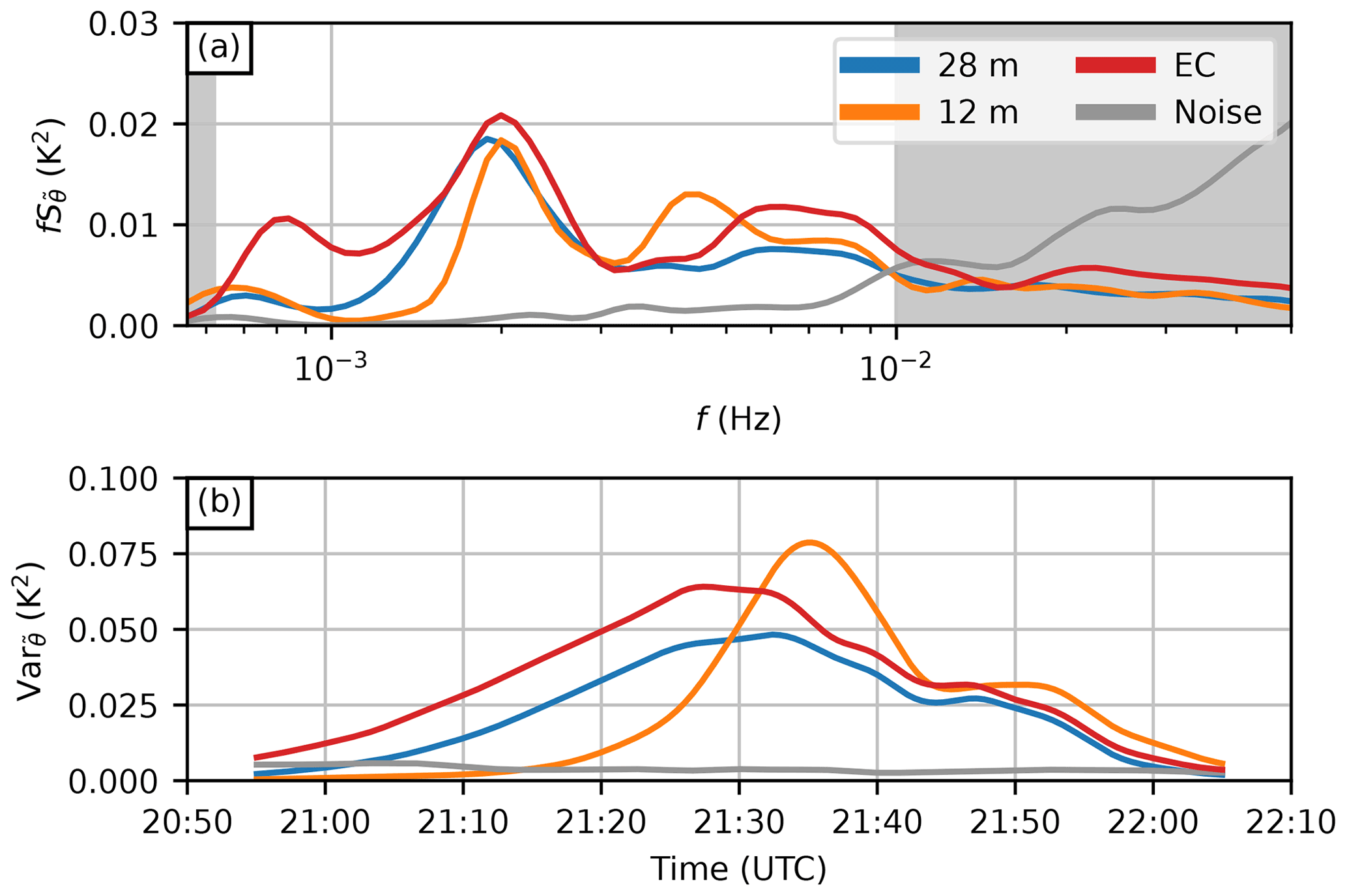
Figure 10 Wavelet analysis for the event on 27 January 2020. (a) Wavelet-derived temperature spectral energy density for DTS $\stackrel{\mathrm{̃}}{\mathit{\theta }}$ from two heights and for EC T_s. (b) Corresponding band-passed wavelet variance of temperature, including variance contributions from only the unshaded area of (a). Five-minute running-average smoothing has been applied in (b). The noise is the estimated average DTS noise at the two heights.

Reconstructing a band-passed ($\mathrm{6.2}\times {\mathrm{10}}^{-\mathrm{4}}$ Hz < f < $\mathrm{1.0}\times {\mathrm{10}}^{-\mathrm{2}}$ Hz) variance from the wavelet transforms (Fig. 10b) reveals a difference in the processes at 28 and 12 m. The event is shorter lived, with higher peak thermal turbulence intensity at the lower level: the 28 m and EC variances have relatively smooth appearances between 21:05–21:45 UTC, whereas the 12 m variance increases rapidly from 21:20 UTC to peak at 21:36 UTC and extends until 21:45 UTC, after which all three variances behave similarly. It is also worth noting that, whereas the onset of thermal turbulence at 12 m is much faster and delayed compared to that at 28 m, the decrease in the intensity after 21:50 UTC follows a relatively similar path at both heights.

This overall behaviour of the frontal passage can be explained with the help of these findings; during the onset phase, the profile is increasingly stable, with the inversion decoupling the flow at the two heights, and no gusts are able to mix the profile to neutral. However, towards the end of the event, as the warm airmass mixes downwards, some gusts are able to mix the whole profile, which increases the overall turbulent mixing across the profile. Mixing effectively increases the decay in the inversion strength, which in turn reduces the amount of negative buoyancy that a warm gust has to work against, increasing the coupling of the flow across the inversion. This can be seen as increased peak variance, shorter duration of the event (higher k and a narrower variance peak), and stronger fluctuations in the observed B as the inversion progresses towards the ground. However, as no increase in the downward propagation of the inversion can be observed from the t₀ profile despite the shorter duration of the event, the depth of the inversion layer has to decrease towards the ground to compensate. This seems reasonable, as the eddy sizes associated with the mixing gusts scale with height in the surface layer, reducing the vertical length scale of the eddies as the inversion layer approaches the ground. At z<6 m, k decreases, possibly due to the influence of nearby vegetation or other obstacles.

3.4 Convective boundary layer development during 21–23 April 2020

Our second case study focuses on demonstrating the usability of DTS measurements for understanding convective boundary layer development on three subsequent mornings during 21–23 April 2020 (Fig. 11). All three mornings share a similar environmental setting: NNW to NNE synoptic-scale flow coming over the land, clear skies, and almost-equal inbound solar radiation. However, on 22 and 23 April, a front associated with a sea-breeze cell forming on the northern coast of the Gulf of Finland (caused by differential heating of land and sea surfaces) passes over Helsinki, moving inland. During the passage of the front, the low-level flow turns southerly in Helsinki and at the measurement site. Compared to the air being heated by the land, this southerly flow brings colder surface air from the sea to the coast. The passage of the sea-breeze fronts over the measurement site (the onset of the sea-breeze wind) on 22 and 23 April can be easily identified from the DTS $\stackrel{\mathrm{̃}}{\mathit{\theta }}$ time series (Fig. 12a) as a sudden halt and decline in rising values. The onset of the sea breeze happens at approximately 07:00 UTC on 22 April and almost three and a half hours later, at 09:20 UTC, on 23 April. The overall behaviour of the sea-breeze cell on the northern coast of the Gulf of Finland is beyond the scope of this article (previous studies on this matter include Savijärvi, 1985; Savijärvi et al., 2005; Gahmberg et al., 2010), but the setting provides a good opportunity to study thermal IBL caused by the discrepancy between the cold incoming marine air and the solar-heated urban surface. Additionally, a day with a similar setting except without the formation of a sea breeze, 21 April, provides a good baseline for comparison.

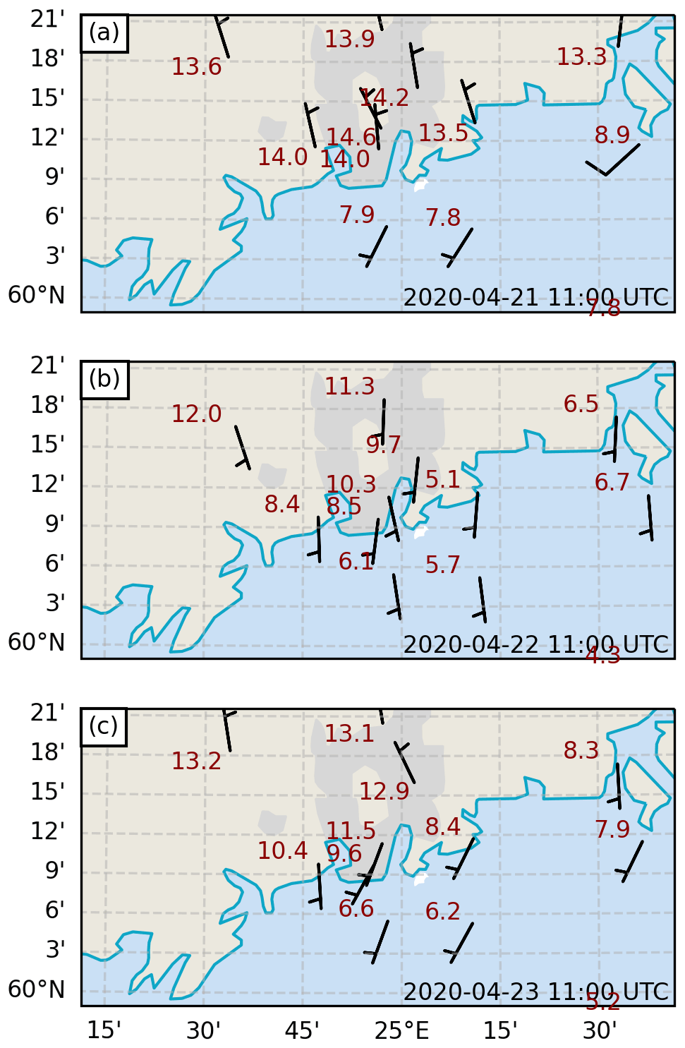
Figure 11 Surface observations of temperature and wind from official weather stations close to Helsinki at 11:00 UTC on (a) 21 April 2020, (b) 22 April 2020, and (c) 23 April 2020.

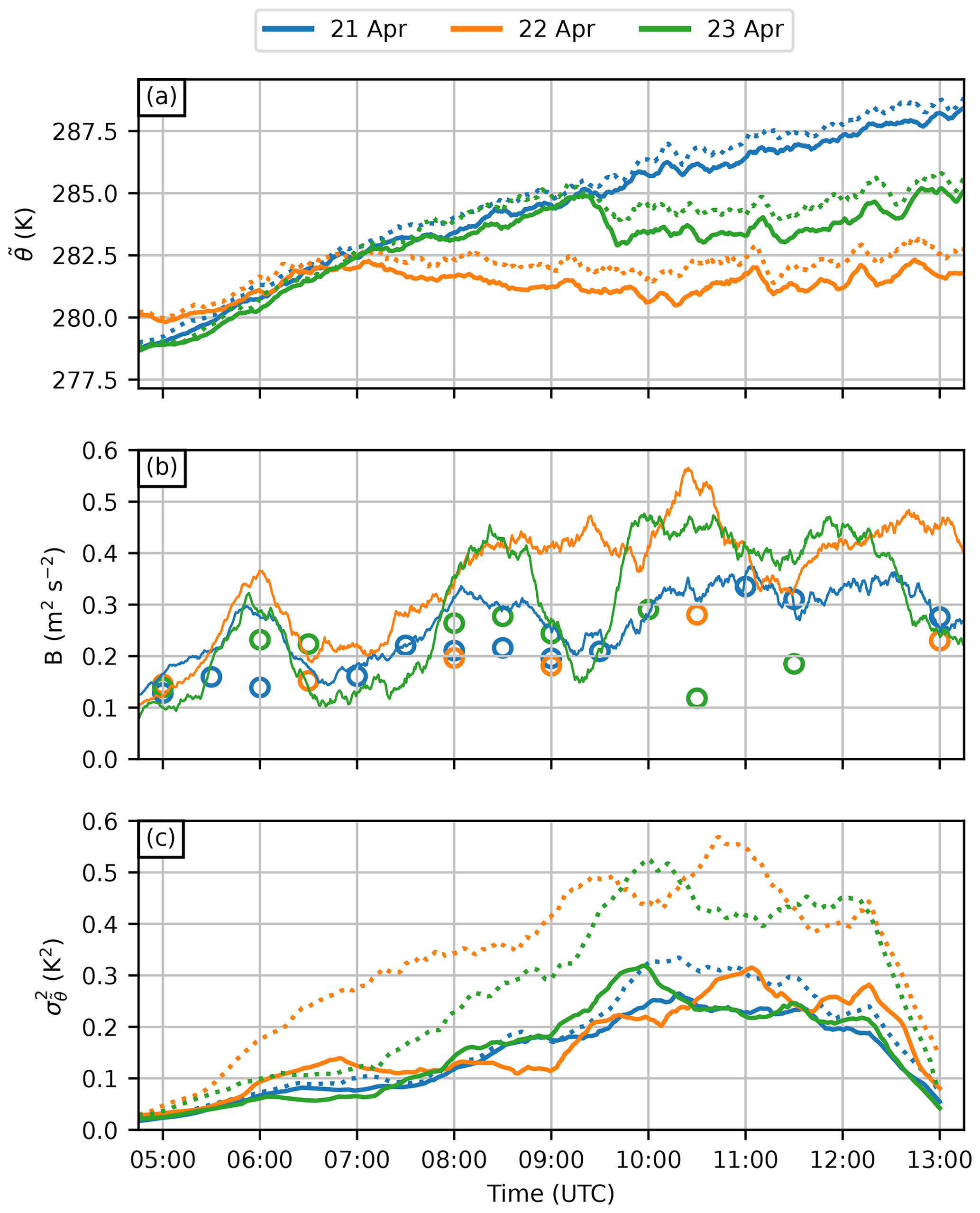
Figure 12 An overview of convective boundary layer development on 21–23 April 2020. (a) Time series of $\stackrel{\mathrm{̃}}{\mathit{\theta }}$ estimated from the DTS system from two heights, 28 m (solid lines) and 6 m (dotted lines). (b) Column-integrated buoyancy observed using the DTS system (solid lines) and predicted using MOST (circles). Some of the predictions are missing due to flux stationarity screening performed on the EC data. (c) Wavelet-estimated localised variance estimates for 28 m (solid lines) and 6 m (dotted lines). Ten-minute moving-average smoothing has been applied to the data in all panels.

The MOST-predicted B (Eqs. 18 and 20) is generally in good agreement with the DTS-observed B during 21 April 2020 (Fig. 12b). There are two peaks not predicted by MOST: those at 05:30–06:30 and 08:00–09:00 UTC, but otherwise the predicted B follows the observed B surprisingly closely, given the assumptions made in MOST. However, for 22 and 23 April 2020, MOST significantly underestimates B after the onset of the sea breeze. This indicates that the observed profile was more unstable than that predicted with the EC-estimated ζ and MOST. Such a discrepancy can be caused by a thermal IBL that has not yet grown to mast top height (Venkatram, 1986; Garratt, 1990). Figure 12c gives more indication of a developing IBL; the temperature variance at 6 m increases significantly after the onset of the sea breeze. A similar increase is not seen at 28 m, further indicating the presence of a thermal IBL caused by the differential surface heating between urban and sea surfaces. Investigating these observed temperature profiles individually (Fig. 13) shows that the profiles for each day are very similar to each other above about 12 m. However, the negative gradient of the profiles below about 12 m increases noticeably after the onset of the sea breeze on 22 and 23 April, indicating a possible thermal IBL corresponding to the land and urban surface.

Figure 13 Observed temperature profiles for 21–23 April 2020 during three different averaging windows: (a) before the sea-breeze front has passed, (b) after the front has passed on 22 April but not on 23 April, and (c) after the front has passed the site on 22 and 23 April. The corresponding averaging intervals are given at the top of each panel.

It is also interesting to note that the two peaks in observed B mentioned earlier are common to all 3 d, which could be an indication of local phenomena intrinsic to the location, such as advection of air mixed from a nearby cold air pool, or more general phenomena related to the morning transition itself.

4 Conclusions

We have presented the results of a 14-week measurement campaign utilising high-frequency DTS temperature profile measurements at a coastal urban site, with a focus on the performance of the measurement system in varying meteorological conditions, as previous studies have mainly performed short-term analyses in selected meteorological conditions. Beyond performing statistical analysis over the whole measurement period, we have demonstrated the potential of the setup for studying the surface layer structure in two different meteorological scenarios.

The performance of the DTS system depends heavily on the atmospheric stability. The abundance of near-neutral conditions during the campaign severely affected the overall availability of DTS-estimated turbulence statistics. This was caused by the lack of temperature fluctuations induced by buoyancy effects or mechanical forcing in near-neutral conditions, which resulted in the instrument SNR falling below the threshold required for the reliable estimation of second- or third-order statistical moments. Conditionally sampling a DTS dataset based on SNR produces a dataset that is biased stability-wise and will miss most near-neutral conditions. Therefore, care must be taken when making conclusions based on such datasets. Further instrument development could mitigate this problem, as it is directly dependent on the instrument noise. When data with high enough SNR values are used, it is seen that that the DTS-derived temperature variance matches EC measurements well and that the vertical profile follows MOST-predicted profiles surprisingly well at this complex urban measurement site. This was the first time that the EC measurements were shown to be measuring the constant flux layer despite the relatively short measurement mast at the site.

The first case study, which focused on a warm front mixing event, demonstrated that, through careful investigation of the scales of turbulence associated with the event, it is possible to extract useful information on turbulence and mixing processes from the DTS data, even in low-SNR conditions. In this case, wavelet analysis proved useful, since it allowed an analysis of the scales relevant to the event, which were not impacted heavily by the instrument noise. Additionally, by using column-integrated buoyancy instead of individual measurements at individual heights, it was possible to construct a more comprehensive picture of the behaviour of the temperature profile during a mixing event. The case highlighted the potential of the DTS system to provide new insights into the near-ground mixing of airmasses – a process not well covered by more conventional surface layer measurements.

The second case study, focusing on springtime convective boundary layer development in the presence of a sea-breeze cell, presented the possibilities for investigating the surface layer structure in the presence of an IBL with DTS. We demonstrated that DTS can capture the modification of the temperature profile due to differential surface heating between urban and sea surfaces. For the non-sea-breeze case, the surface layer profile is predicted well by measurements higher in the ISL and by MOST, but is not predicted well in the presence of a sea-breeze cell. Hence, DTS measurements will help in developing better parametrisations for surface layer flows, which are required for improving the prediction of near-surface temperatures by numerical weather forecast and climate models.

Analyses of surface layer structure and turbulence often incorporate simultaneous knowledge of both the temperature and wind profiles and/or their horizontal variations. Our decision to measure only the temperature profile, supplemented by a sonic anemometer at one height, reduced the potential for further analyses of the surface layer. Hence, for further studies, we recommend supplementing the DTS profile measurements with sonic anemometers at multiple heights for evaluating other aspects of the surface layer such as turbulence production via wind shear. Furthermore, using a taller measurement mast would also aid interpretation of the surface layer structure (RSL and IBL) in varying meteorological conditions.