Quantification and mitigation of the instrument effects and uncertainties of the airborne limb imaging FTIR GLORIA

The Gimballed Limb Observer for Radiance Imaging of the Atmosphere (GLORIA) is an infrared imaging FTS (Fourier transform spectrometer) with a 2-D infrared detector that is operated on two high-flying research aircraft. It has flown on eight campaigns and measured along more than 300 000 km of flight track.

This paper details our instrument calibration and characterization efforts, which, in particular, almost exclusively leverage in-flight data. First, we present the framework of our new calibration scheme, which uses information from all three available calibration sources (two blackbodies and upward-pointing “deep space” measurements). Part of this scheme is a new algorithm for correcting the erratically changing nonlinearity of a subset of detector pixels and the identification of the remaining bad pixels.

Using this new calibration, we derive a 1σ bound of 1 % on the instrument gain error and a bound of 30 nW cm⁻² sr⁻¹ cm on the instrument offset error. We show how we can examine the noise and spectral accuracy for all measured atmospheric spectra and derive a spectral accuracy of 5 ppm on average. All these errors are compliant with the initial instrument requirements.

We also discuss, for the first time, the pointing system of the GLORIA instrument. Combining laboratory calibration efforts with the measurement of astronomical bodies during the flight, we can achieve a pointing accuracy of 0.032^∘, which corresponds to one detector pixel.

The paper concludes with a brief study of how these newly characterized instrument parameters affect temperature and ozone retrievals. We find that the pointing uncertainty and, to a lesser extent, the instrument gain uncertainty are the main contributors to the error in the result.

1 Introduction

The upper troposphere/lowermost stratosphere is a region with a strong chemical contrast and highly differentiated vertical structure. Its composition is determined by various processes, e.g., convection, lightning, biomass burning, aircraft exhaust, and stratosphere–troposphere exchange (Holton et al., 1995). It also heavily influences the surface climate due to its impact on radiative transport (de F. Forster and Shine, 1997; Riese et al., 2012; Xia et al., 2018). Historically, satellite limb sounding instruments have served us well for observing this atmospheric region (e.g., Hegglin et al., 2009, 2021). A closer and more highly resolved view is achieved by moving the measuring instrument much closer to the region of interest. Airborne limb sounders allow the high measurement density needed to resolve fine structure (e.g., Krasauskas et al., 2021).

Principally, limb sounders offer high vertical resolution but lack

horizontal resolution, as the technique does not allow the resolution of structures along the lines of sight of the instrument. Besides 2-D cross sections along the flight path, the Gimballed Limb Observer for Radiance Imaging of the Atmosphere (GLORIA; Riese et al., 2014; Friedl-Vallon et al., 2014) also allows the tomographic reconstruction of limited volumes of interest (e.g., Ungermann et al., 2011; Krisch et al., 2017) by combining measurements taken in different azimuthal view directions, thereby overcoming the conventional limitations of the measurement technique.

The GLORIA instrument has been flown successfully on several measurement campaigns ranging from TACTS/ESMVal in 2012 (e.g., Rolf et al., 2015) to PGS in 2015/2016 (e.g., Woiwode et al., 2018), StratoClim (e.g., Höpfner et al., 2019), WISE (e.g., Kunkel et al., 2019) in 2017, and the most recent SouthTRAC campaign in 2019 (Johansson et al., 2021). During 600 flight hours in total on 75 scientific flights, GLORIA collected more than 120 TiB of data, providing ≈300 000 km of atmospheric profiles and many volumes resolved in three dimensions. The quality of the measured infrared radiances was sufficient from the beginning to allow the retrieval of temperature and strongly emitting trace gases from TACTS/ESMVal onward (e.g., Ungermann et al., 2015; Woiwode et al., 2015; Johansson et al., 2018).

Over the course of processing and evaluating data from these campaigns, our understanding of the instrument has constantly improved (Kleinert et al., 2014; Guggenmoser et al., 2015; Kleinert et al., 2018). We have consequently adapted and standardized our in-flight calibration scenario. As the instrument behaves differently when it is onboard the aircraft than when it is in the laboratory, we are increasingly focusing on the sole use of in-flight data for characterization efforts. Also, the continuously growing dataset provides an excellent basis for profound in-flight instrument characterization.

The structure of this paper is as follows. The first part starts with a brief instrument description and introduces the current calibration and processing scheme for converting GLORIA measurements to radiance spectra by exploiting all three available calibration sources: the two onboard calibration blackbodies and the upwards-pointing “deep space” measurements. This includes a correction for the nonconstant nonlinearity of several detector pixels as well as the identification of bad pixels and some other effects.

Second, we use the in-flight measurements to quantify the major error sources, or at least to derive the upper bounds of these errors, and to characterize important instrument parameters such as the relative and absolute radiance accuracy, radiance precision (noise equivalent spectral radiance; NESR), spectral accuracy, line of sight, and point spread function.

Third, we briefly discuss the impact of the characterized errors on level 2 products using a simple temperature and ozone retrieval as an example. As such, this study collects all relevant processing information for GLORIA in one place, making it a reference for further geophysical interpretation of the data or derivative satellite-borne instruments.

2 The GLORIA instrument

The GLORIA instrument consists of a spectrometer and a gimbal mount that stabilizes the spectrometer in the airborne environment and allows the instrument's line of sight (LOS) to be pointed either at the atmospheric limb, at a 10° upward angle, at nadir, or at one of the two integrated blackbody calibration sources. The spectrometer combines a classical Michelson interferometer with a two-dimensional detector, allowing up to 16 384 interferograms (128×128) to be taken simultaneously. In the typical configuration, we use 128 vertical by 48 horizontal pixels for a total of 6144 interferograms. The Michelson interferometer can be configured for a maximum optical path difference of up to ±8 cm, which corresponds to a spectral sampling of 0.0625 cm⁻¹. The instrument uses a cryogenic HgCdTe detector array for the detection of infrared radiation in the spectral range between 780 and 1400 cm⁻¹. We focus on this range in our analysis. Outside this range, the data quality deteriorates quickly but is sometimes still useful for retrievals. Thus, we usually show the slightly larger spectral range from 750 to 1450 cm⁻¹. Atmospheric measurements are typically taken in one of the three operating modes listed in Table 1, which have differing trade-offs between temporal/spatial and spectral resolution. A schematic of the instrument is shown in Fig. 1.

Table 1 Typical operating modes of GLORIA. The actual optical path difference is typically longer than the nominal one. Approximate values for the temporal resolution are given as it partially depends on the configuration of the instrument.

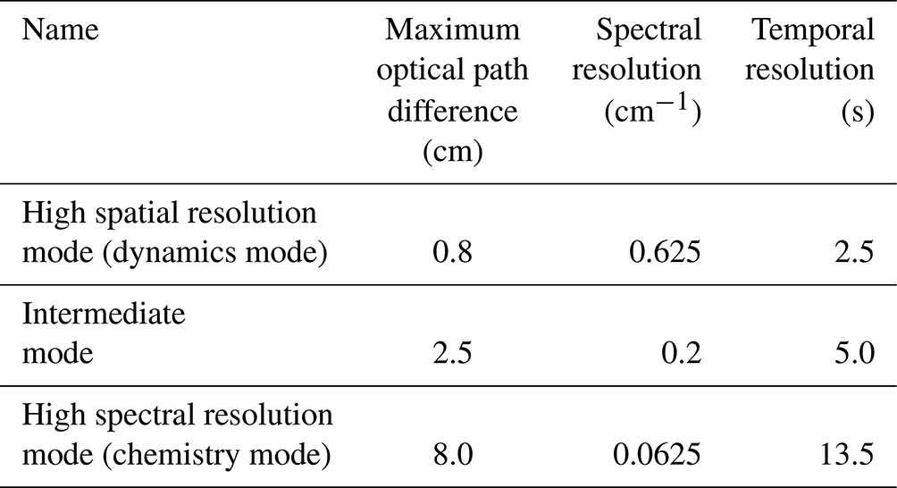
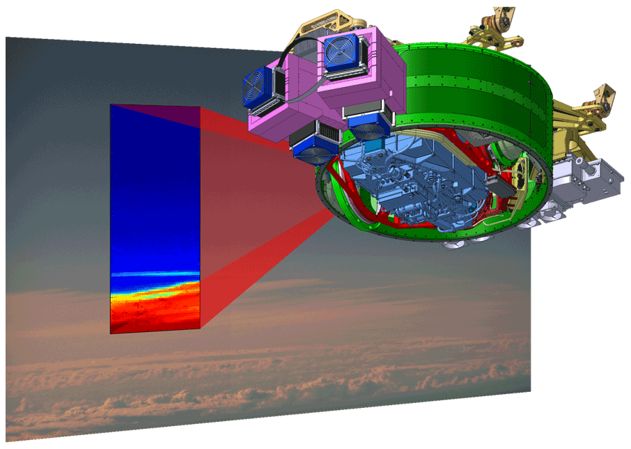
Figure 1 Schematic of the instrument and the measurement principle. Depicted is an overlay of an IR and a visual image together with a technical drawing of the instrument.

The whole spectrometer is cooled with solid carbon dioxide (dry ice) to about 220 K in order to reduce the self-emission from the instrument and thus enhance the signal-to-noise ratio. A detailed description of the concept of the instrument was published by Friedl-Vallon et al. (2014).

The processing chain of GLORIA encompasses the usual level 0 to level 2 structure. The raw radiance measurements are digitized with 14 bit A/D converters and stored in a proprietary binary format in combination with time stamps of zero crossings of a reference laser that allow for highly accurate determination of the optical path difference of the image. The level 0 processing step then transforms the measured data (evenly sampled in time) to proper interferograms (evenly sampled in optical path distance). This step includes both a nonlinearity correction based on laboratory characterization of the used detector array and a Shannon–Whittaker resampling, as presented by Brault (1996). During the resampling step, the spectral axis of each pixel is scaled according to its off-axis angle in order to account for the dependence of the actual optical path difference (OPD) on the angle between the light observed at a detector pixel and the optical axis of the instrument. We typically apply a strong Norton–Beer apodization to all our interferograms unless specified otherwise (Norton and Beer, 1976, 1977). The level 1 processing step then transforms the interferograms into spectra by means of a Fourier transformation and compensation of the instrument gain and offset using the complex calibration approach presented by Revercomb et al. (1988). These processing steps have been described in detail by Kleinert et al. (2014) and Guggenmoser et al. (2015). The level 2 processing step uses the calibrated spectra to determine geolocated temperatures, trace gas volume mixing ratios (VMRs), and ancillary information, e.g., about aerosol load and cloudiness, by means of inverse modeling. In practice, the assumed atmospheric state is varied until simulated measurements for that state agree with the actual measurements. Two different level 2 processors are used for evaluating GLORIA data, depending on the recorded spectral resolution. These have been described by Ungermann et al. (2015) for high spatial resolution measurements and Johansson et al. (2018) for high spectral resolution measurements (see Table 1).

3 Radiometric calibration concept

Here, we introduce the overall concept of our revised calibration scheme before describing individual parts in detail in the following sections.

Radiometric calibration is the central step of level 1 processing. This maps the Fourier-transformed interferograms (raw complex spectra with arbitrary units) to proper physical quantities. It also includes the removal of all signatures of the instrument's self-emission (Revercomb et al., 1988).

GLORIA is operated in an open compartment below the aircraft, and environmental temperatures can range between less than 230 K and more than 300 K. The self-emission of the interferometer is significant and changes over time, which requires calibration measurements to be taken in flight. For this purpose, the instrument is equipped with two blackbodies that can be actively heated, cooled, or stabilized at a desired temperature (Olschewski et al., 2013). In order to avoid ice contamination and optimize the power budget, the “cold” blackbody is stabilized at about 0–10 K below ambient temperature, while the “hot” blackbody is heated to 30–40 K above the cold blackbody. A third calibration source is provided by “deep space.” Here, the instrument is pointed upwards at an elevation angle of 10^∘ to measure the dark background of space. If the carrier was not flying so low that atmospheric emissions cannot be neglected, this would effectively deliver a direct measurement of the instrument offset L_o. In Sect. 4.1, we describe our current method for removing the remaining emission lines to approximate a true deep space measurement. In principle, two calibration sources would be sufficient for the radiometric calibration, so the use of three sources allows for redundancy and validation.

The deep space measurements have to be recorded in high spectral resolution mode in order to resolve atmospheric features, while blackbody measurements can be recorded in high spatial resolution mode at one-tenth of the full spectral resolution and are thus much less time consuming to take. Therefore, we take deep space measurements only about once per hour, while measurements of the two blackbodies are recorded about every 15 min. In order to enhance the signal-to-noise ratio (SNR), 10 spectra for each blackbody (requiring ≈25 s in total) and 6 deep space spectra (requiring ≈85 s in total) are taken.

We follow the approach of Revercomb et al. (1988) in that we can transform our uncalibrated complex spectra with arbitrary units to calibrated complex spectra using a multiplicative gain and an additive offset term. The uncalibrated spectra are necessarily complex due to the Fourier transformation of our asymmetric real interferograms. Even perfectly calibrated spectra are still complex, as part of the (asymmetric) measurement noise is mapped to the imaginary plane. With L∈ℝ the radiation measured by the instrument, g∈ℂ the complex gain, and L_o∈ℂ the offset (largely caused by the self-emission of the interferometer), the measured signal S∈ℂ can be obtained via

$$\begin{array}{}\text{(1)}& S=g\left(L+L_{\mathrm{o}}\right).\end{array}$$

These terms are all functions of both the detector pixel (u,v) and wavenumber ν of the spectral sample.

Assuming the response of the detector to be linear with respect to the incoming photon flux (see also Sect. 4.2), the gain g and offset L_o may be determined from two uncalibrated measured spectra S₁∈ℂ and S₂∈ℂ of blackbody radiation sources with known emission characteristics as follows:

$$\begin{array}{}\text{(2)}& g={\displaystyle \frac{S_{\mathrm{2}}-S_{\mathrm{1}}}{B\left(T_{\mathrm{2}}\right)-B\left(T_{\mathrm{1}}\right)}}\end{array}$$

and

$$\begin{array}{}\text{(3)}& L_{\mathrm{o}}={\displaystyle \frac{S_{\mathrm{1}}}{g}}-B\left(T_{\mathrm{1}}\right)={\displaystyle \frac{S_{\mathrm{2}}}{g}}-B\left(T_{\mathrm{2}}\right),\end{array}$$

where B is the Planck function and T is the temperature of the corresponding blackbody. If the deep space spectrum S_d is used as one blackbody spectrum, the radiation from this source is (effectively) zero, and Eqs. (2) and (3) simplify to

$$\begin{array}{}\text{(4)}& g={\displaystyle \frac{S_{\mathrm{1}}-S_{\mathrm{d}}}{B\left(T_{\mathrm{1}}\right)}}\end{array}$$

and

$$\begin{array}{}\text{(5)}& L_{\mathrm{o}}={\displaystyle \frac{S_{\mathrm{d}}}{g}}={\displaystyle \frac{S_{\mathrm{1}}}{g}}-B\left(T_{\mathrm{1}}\right).\end{array}$$

As shown by Kleinert et al. (2018), the calibration parameters determined by two blackbodies with a rather small temperature difference are more susceptible to errors (e.g., in blackbody temperature or homogeneity) than a combination of one blackbody and a deep space measurement. Since the radiance from the cold blackbody is closer to (but still above) the radiation from the atmosphere, it is better suited for the determination of the gain function than the hot blackbody is. We therefore determine the gain once every hour from the cold blackbody and the deep space measurements.

We found that the gain magnitude, which is governed by the sensitivity of the detector array, is very stable during any given flight (see Sect. 5.2). Therefore, one median gain magnitude is determined for each flight. The phase of the complex gain function varies depending on the direction of the moving slide during interferogram acquisition (“forward” or “backward”), but it also slowly changes with time because of the thermal variations of the instrument. Therefore, the phase is linearly interpolated in time between the calibration measurements.

The offset of the instrument is dominated by its thermal self-emission and changes during the flight, along with the changing temperature of the instrument. When the gain is known, the offset can be calculated from this gain and the spectrum of one calibration source. Since the blackbody spectrum is recorded much faster and is thus recorded more frequently, we use the gain and the cold blackbody measurements to determine the instrument offset every 15 min. Between the calibration measurements, the offset is linearly interpolated in time, except for the contribution of the outer entrance window (see Sect. 4.3).

The main differences from the calibration method described by Kleinert et al. (2014) are the use of a technique for removing atmospheric emissions from deep space spectra (see Sect. 4.1), an improved nonlinearity correction (see Sect. 4.2), and the averaging of the gain magnitude over the flight and the real part of the offset over the forward and backward sweep directions.

4 Methods

This section presents methods developed to account for the effects of a real instrument at (comparatively) low flight altitudes. For each effect, we will first give a short explanation of the physical cause and then detail the method developed to compensate and characterize this effect in the calibration process.

4.1 Removal of atmospheric contribution to calibration spectra

For satellite measurements, the instrument's self-emission can be measured by directly looking into true deep space with effectively zero radiance. Due to GLORIA's position below the aircraft, the maximum elevation angle of its optical axis is ≈10^∘ above the horizon.

There is still a considerable amount of atmosphere in the line of sight of deep space measurements taken at a 10^∘ angle while flying at an altitude below 15 km. In order to remove the atmospheric radiance emitted by the air within this line of sight, we use atmospheric retrieval techniques to best model the atmospheric contribution to the measured signal and then subtract the forward-calculated atmospheric spectrum from the measured one. This removal of atmospheric features from the smooth instrument offset is called shaving.

As a starting point, we calibrate the deep space measurements using gain and offset functions derived from measurements of the two onboard blackbodies. The median spectrum over the whole detector array is used for the representation of the radiance of the central pixel. This is justified by the observation that the radiance variation over the detector field at this upward-pointing elevation angle is rather linear with respect to the elevation angle or pixel row. The median is insensitive to outliers and hence bad pixels have a negligible impact on the result.

The forward calculation of the spectra requires a priori assumptions about the atmospheric state, i.e., pressure, temperature, and the VMRs of the relevant trace gases emitting in the spectral range covered by the measurements. Pressure, temperature, H₂O, and O₃ are taken from ECMWF analysis data (e.g., Dee et al., 2011) linearly interpolated to the measurement location and time. The other trace gas profiles are taken from a standard atmosphere (see Appendix E). Forward calculation and retrieval are performed with the radiative transfer model KOPRA (Karlsruhe Optimized and Precise Radiative transfer Algorithm; Stiller, 2000) and the retrieval software KOPRAFIT (Höpfner et al., 1998).

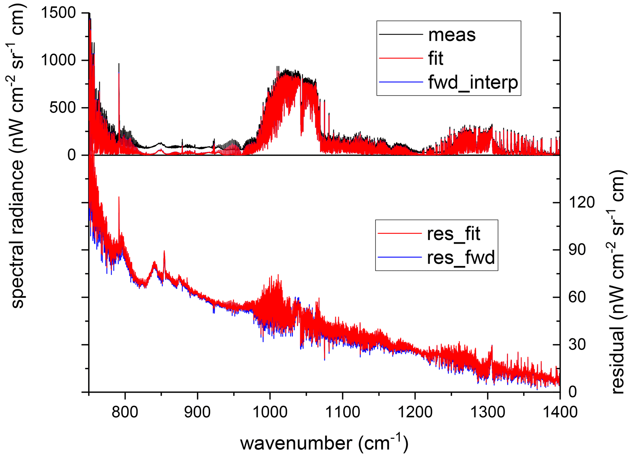
Figure 2 Original measured spectrum without subtraction of the Planck function (black), forward-calculated spectrum from the fit results (red), and linearly interpolated spectrum from the forward calculations for the lowermost and uppermost detector rows (blue, hidden by the red line). The lower panel shows the residuals (measured minus fit in red and measured minus interpolated forward calculation in blue) enlarged by a factor of 10, demonstrating the very small difference between the fitted and forward-calculated interpolated spectra.

The goal is to model as well as possible the atmospheric contributions present in the measured deep space spectra in order to unveil the instrument's self-emission. The actually retrieved temperature and trace gas profiles are not employed further, as this model is tuned to fit the measurements optimally and not to derive realistic atmospheric parameters. The atmospheric spectrum is modeled in the spectral range from 750 to 1400 cm⁻¹, allowing for good calibration quality slightly outside the specified spectral range starting at 780 cm⁻¹ too.

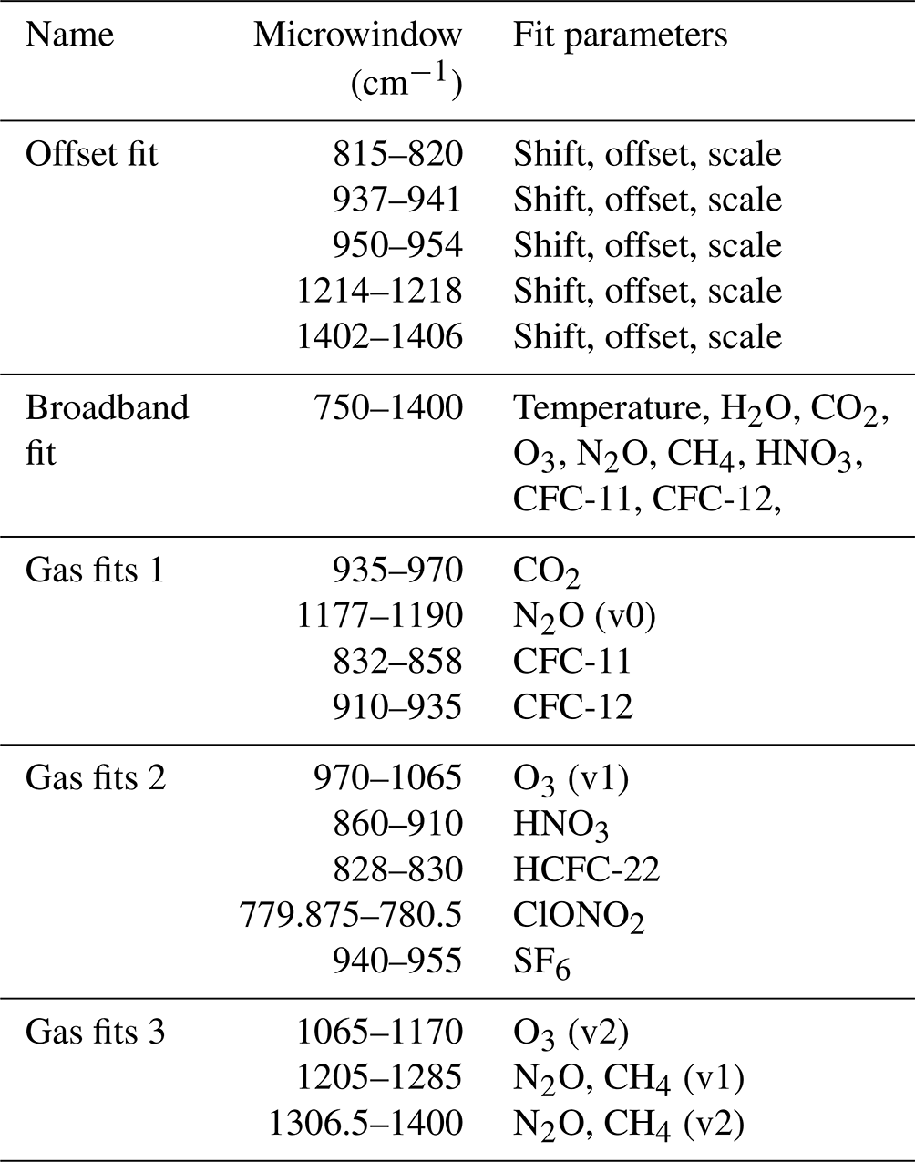
The fit is performed iteratively. First, a residual radiance offset is fitted and subtracted from the measured spectrum. In the next step, a broadband fit is performed with temperature and eight gases (H₂O, CO₂, O₃, N₂O, CH₄, HNO₃, CFC-11, and CFC-12) as fit parameters. In total, 29 gases are used in the forward calculation. The fit is then refined by fitting single gas profiles in dedicated microwindows in several iterations. The gases and iterations are shown in Table 2, and are described in more detail in Appendix A.

Table 2 Microwindows and fit parameters used in the different iterations of the fitting process. The gases considered in the forward calculation using the a priori profiles are H₂O, CO₂, O₃, N₂O, CH₄, O₂, SO₂, NO₂, HNO₃, ClO, OCS, HOCl, N₂, HCN, CH₃Cl, H₂O₂, C₂H₂, COF₂, CFC-11, CFC-12, HCFC-22, SF₆, CFC-14, CCl₄, CFC-113, CFC-114, N₂O₅, ClONO₂, and HNO₄. Furthermore, the continuum of O₂ and H₂O is considered. For further details, see the text.

The fit results are then used for a forward calculation over the whole spectral range. The measured spectrum and the forward calculation are shown in Fig. 2 in black and red, respectively. The residual shown in the lower part of the figure (red) reveals the quality of the removal of atmospheric signatures. The residual is dominated by the Planck-like offset and some broadband structures below 850 cm⁻¹, which can be attributed to the germanium entrance window. The remaining atmospheric features are reduced to the order of 10 nW cm⁻² sr⁻¹ cm for most of the spectral range.

The forward-calculated spectrum is valid for the central row of the detector because the median over the array has been fitted. Although the variation with elevation angle is rather small for the upward-looking measurements, it is not negligible. Therefore, forward radiative-transfer calculations are performed for elevations of +8 and +12^∘, corresponding to the lowermost and uppermost detector rows, respectively. For the rows in between, these spectra are linearly interpolated. The linearly interpolated spectrum for the central row is also shown in Fig. 2, in blue. The difference from the red spectrum (forward calculation for an elevation angle of +10^∘) is only distinguishable in the residual plot, showing that the differences due to the interpolation are much smaller than the remaining atmospheric features and are therefore negligible.

The removal of atmospheric features from the uncalibrated spectra is done for each pixel individually by interpolating the forward-calculated spectra to the corresponding row and multiplying this spectrum by the gain function of the corresponding pixel, using the gain that was determined from the two blackbody measurements. Several small sections of the spectrum are then linearly interpolated from the neighboring spectral samples because of the remaining atmospheric features present (namely the Q-branches of CO₂, HNO₃, and CH₄) or spikes in the spectrum at distinct known frequencies due to electrical noise.

The uncertainty of the instrument offset determination is estimated from the difference between the measurement after subtracting the broadband offset and the forward calculation. It is estimated to be 20 nW cm⁻² sr⁻¹ cm (2σ). More details about this uncertainty estimation are given in Appendix A.

4.2 Detector nonlinearity correction

The detector is subject to nonlinearity, i.e., a change in sensitivity depending on the overall photon load. In a first-order approximation, this effect causes a scaling of the derived spectra that depends on the photon load of the scene (see Appendix B for more details).

As described by Kleinert et al. (2014), the nonlinearity of the detector has been characterized by carefully performing dedicated measurements of a constant source while varying the integration time on the ground. From these measurements, one correction curve for all pixels was determined. This curve works well for most pixels, but a considerable number of pixels show spontaneous changes in their nonlinear behavior, meaning that the derived correction is unsuitable for those pixels. We attribute this to the different thermal expansion coefficients of the detector material and the silicon substrate, leading to make-and-break contacts (Perez et al., 2005). In earlier data versions, these pixels were simply filtered out, but rigorous filtering leads to a considerable decrease in the number of usable pixels. Therefore, we developed a method to determine the correct gain for these pixels as well. Extending the work of Guggenmoser et al. (2015), we constructed an algorithm to exploit the smoothness of the instrument offset L_o to correct the faulty pixels.

As the instrument is focused at infinity, the instrument offset must be a spatially smooth function, as any features in the image from objects residing within the instrument are effectively folded with a Gaussian with a very large support. Thus, we assume that any spatial discontinuities in L_o are caused by the uncorrected nonlinearity of the involved pixels. The assumption of spatial smoothness was exploited by Guggenmoser et al. (2015) to improve upon the offset without also correcting the gain.

The nonlinearity causes, in a first-order approximation, a scaling of the affected spectra. The atmospheric and deep-space measurements are reasonably close in photon load and thus behave in a very similar fashion. In contrast, blackbody measurements have a much stronger signal and scale differently for the problematic pixels. Thus, we use a nonlinear fit to estimate pixelwise scalar nonlinearity scaling factors for the blackbody measurements (see Appendix B for details). We derive these nonlinearity scaling factors for adjusting the blackbody spectra such that the offset L_o is free from discontinuities over the whole spectral range. A set of such derived nonlinearity scaling factors is depicted in Fig. 3. An irregular, clustered distribution of bad pixels is clearly visible. The uncertainty in determining these factors is slightly larger in the circular region, where the instrument offset is close to zero for most of the spectral range. The uncertainty in determining the factors is of the order of one-third to one-half of a percent. Comparing the values derived from the forward and backward sweep directions suggests an uncertainty of ≈0.5 % on average. Figure 4 shows the histogram of derived correction factors. The factors cluster around a value of 1, with a Laplacian-like distribution in the center. However, there are a significant number of pixels with strong nonlinearity in the 5–10 % region.

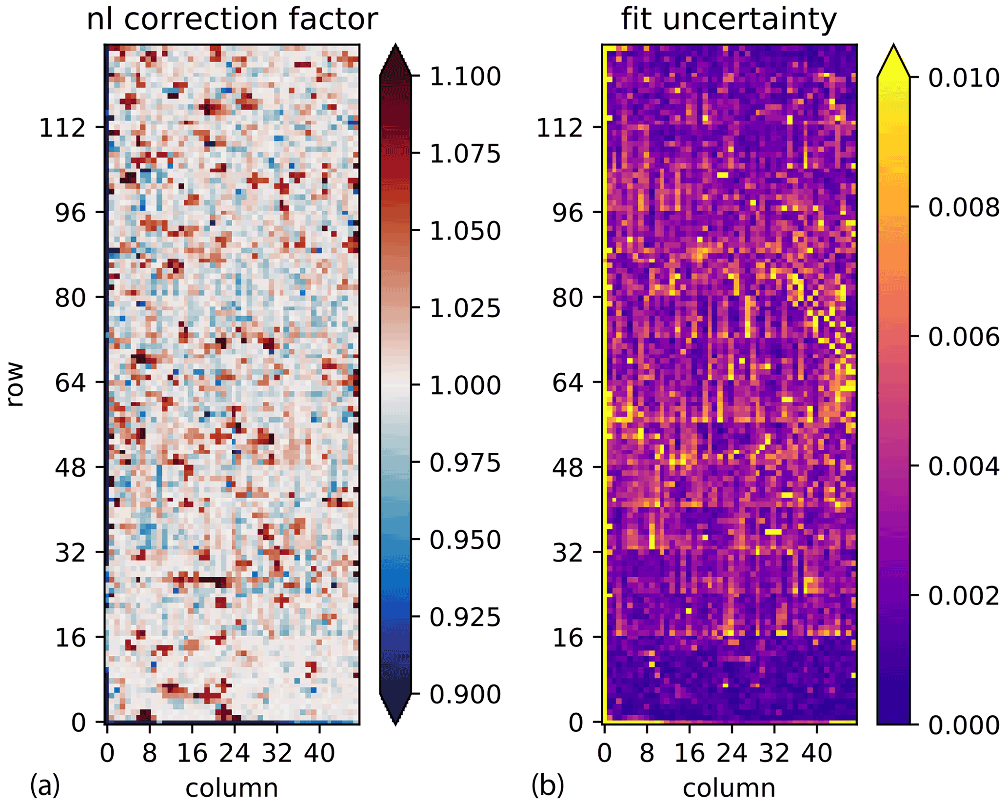
Figure 3 The correction factors for blackbody raw spectra derived for a blackbody–deep space calibration sequence of WISE campaign/flight 16. Panel (a): the correction factors. Panel (b): the uncertainties derived from the least squares fit.

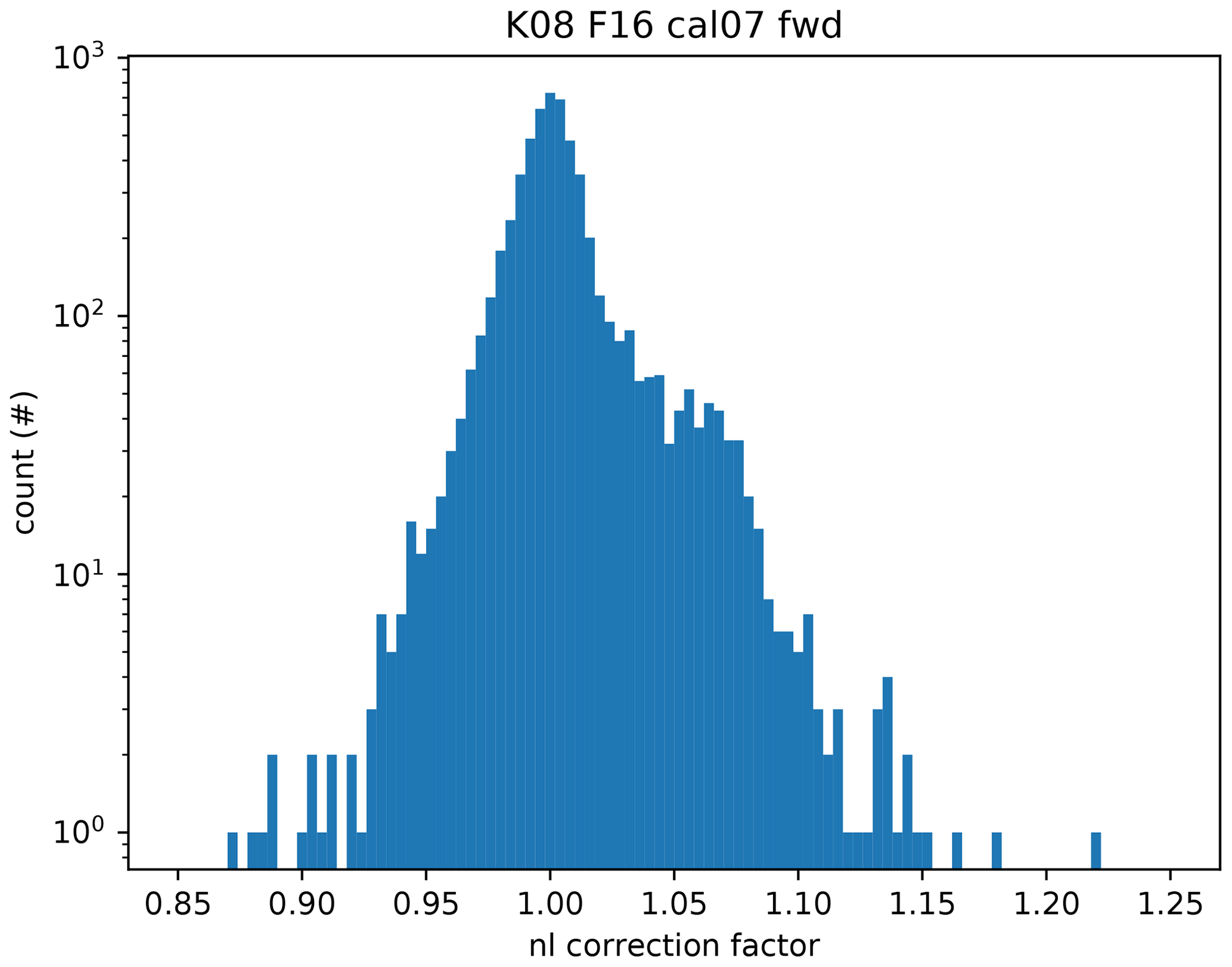
Figure 4 The frequencies of different nonlinearity correction factors derived from one calibration sequence on a logarithmic scale.

The nonlinearity correction factors are derived for each calibration sequence containing a deep space measurement, but are also applied to blackbody measurements in between by linear interpolation in time. As the nonlinear behavior is known to change between flights, it may also change within a flight. We thus analyze a subset of atmospheric spectra for calibration artifacts. Excluding clouds, atmospheric spectra are typically spatially smooth as well.

Using a similar method to that described above, we now determine a scaling factor for the gain function. With a perfect correction or instrument, a value of 1 is expected for all pixels. Differences from 1 can be interpreted as the remaining error in the gain after nonlinearity correction. Analysis of a set of 158 atmospheric measurements uniformly distributed over flight 16 of the WISE campaign gives Fig. 5. The determined scaling errors are much lower than the correction factors applied to the raw blackbody spectra. Only the lowermost rows show large errors; these interferograms taken at lower altitudes already exhibit a mean value that is sufficiently different from those of deep space measurements to have a slightly different sensitivity to incoming radiation due to nonlinearity compared to the deep space spectra.

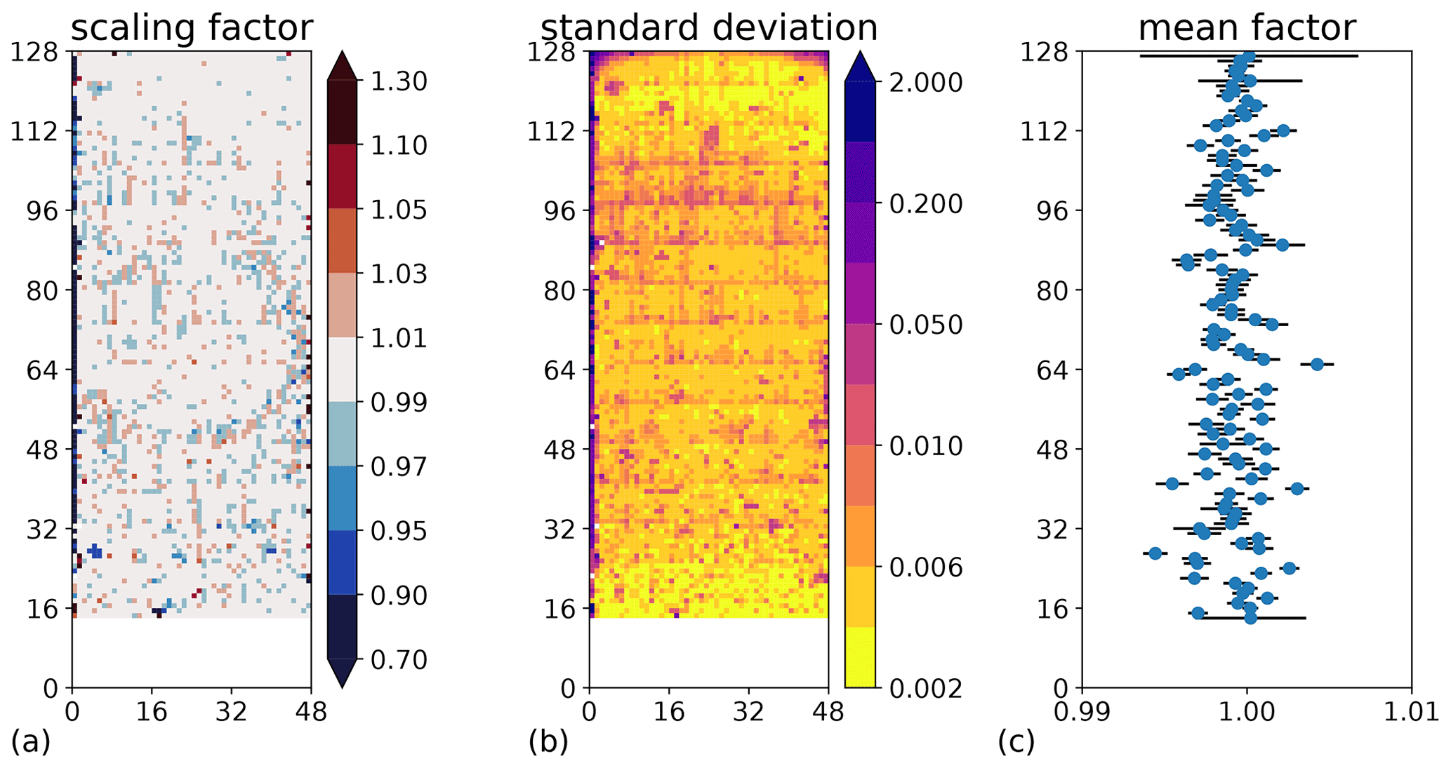
Figure 5 The estimated error in the gain, as derived from the homogeneity of 158 atmospheric spectra. Panel (a): residual scaling factors for each pixel. Differences from one denote the estimated error. Panel (b): the corresponding standard deviation of the variability over the same atmospheric spectra. Panel (c): the estimated error in the gain after averaging over all pixels in a row (excluding the leftmost two and the rightmost columns). All atmospheric spectra were cloudy in the lowermost rows, precluding an analysis.

The resulting row-averaged scaling errors are within ±1 %; some of the largest differences are due to individual pixels of high variability and the rows where (colored) noise is generally quite high. The standard deviation of the remaining error in the gain averaged over rows can thus be computed as ≈0.2 %.

4.3 Outer-window emission correction

The entire instrument, including all windows, is calibrated in flight using deep space and blackbody measurements. Thus, the emission and absorption by the windows should be removed by the calibration process. However, if temperatures change rapidly compared to the calibration frequency of about 15 min, the fundamental assumption of a constant instrument offset L_o during the acquisition of calibration spectra does not hold anymore. The only critical component in this context is the entrance window of the spectrometer, because only this component changes its temperature rapidly with respect to the calibration frequency. Especially during ascent, the temperature changes at a rate of up to 2 K min⁻¹, while the temperature changes of all other components are typically below 200 mK min⁻¹. The instrument gain is computed from calibration sequences with a stable instrument and window temperature and averaged over the flight such that only the instrument offset is affected by this problem.

The spectral emission signature of the germanium window is deduced from in-flight measurements taken at the beginning of the flight, when the window temperature changes rapidly while the temperature of the rest of the instrument stays rather constant. We attribute the difference in measured instrument offset between the first two calibration sequences to the change in the window temperature and calculate the emissivity of the outer germanium window as

$$\begin{array}{}\text{(6)}& \mathit{ϵ}={\displaystyle \frac{L_{\mathrm{o}\mathrm{1}}-L_{\mathrm{o}\mathrm{2}}}{B\left(T_{\mathrm{1}}\right)-B\left(T_{\mathrm{2}}\right)}},\end{array}$$

L_o1 and L_o2 being the calibrated instrument offsets calculated from the first and second calibration sequences, respectively, and T₁ and T₂ being the temperatures of the outer window at the measurement times of the first and second calibration sequences, respectively.

We did this for several flights, discarding outliers and averaging over the rest. The resulting spectral emissivity of the germanium window is shown in Fig. 6. The impact of the germanium window emission is most readily noticeable in the spectral range around 830 cm⁻¹, where the atmospheric signal is very low, but it also affects lower wavenumbers. The window temperature changes too quickly to be captured by the regular calibration measurements after take-off, when the window rapidly cools with the dropping environmental temperature, during and after dive maneuvers, and in situations where the window is exposed to direct sunlight. We also found the window temperature to fluctuate by ≈0.5 K during tomographic measurement patterns, where GLORIA quickly shifts between different azimuth angles and the window is thus subjected to different air flow patterns.

Figure 6 The spectral emissivity of the outer window.

In order to account for these rapid temperature changes of the entrance window, we developed the following approach. Given two calibration measurements at times t₀ and t₁, we compute the instrument offset L_o at time t with $t_{\mathrm{0}}<t<t_{\mathrm{1}}$ by linear interpolation:

$$\begin{array}{}\text{(7)}& L_{\mathrm{o}}\left(t\right)=L_{\mathrm{o},t_{\mathrm{0}}}{\displaystyle \frac{t_{\mathrm{1}}-t}{t_{\mathrm{1}}-t_{\mathrm{0}}}}+L_{\mathrm{o},t_{\mathrm{1}}}{\displaystyle \frac{t-t_{\mathrm{0}}}{t_{\mathrm{1}}-t_{\mathrm{0}}}}.\end{array}$$

We now add a correction term for the window emission in order to retain the measured instrument offsets at times t₀ and t₁ while compensating for the changes in window emission due to the measured window temperature T_win(t) in between. The improved instrument offset $L_{\mathrm{o}}^{*}$ is thus computed as

$$\begin{array}{}\text{(8)}& \begin{array}{rl}{L}_{\mathrm{o}}^{*}\left(t\right)=& \left(L_{\mathrm{o},t_{\mathrm{0}}}+B\left(T_{\mathrm{win}}\left(t_{\mathrm{0}}\right)\right){\displaystyle \frac{\mathit{ϵ}}{\mathrm{1}-\mathit{ϵ}}}\right){\displaystyle \frac{t_{\mathrm{1}}-t}{t_{\mathrm{1}}-t_{\mathrm{0}}}}\\ & +\left(L_{\mathrm{o},t_{\mathrm{1}}}+B\left(T_{\mathrm{win}}\left(t_{\mathrm{1}}\right)\right){\displaystyle \frac{\mathit{ϵ}}{\mathrm{1}-\mathit{ϵ}}}\right){\displaystyle \frac{t-t_{\mathrm{0}}}{t_{\mathrm{1}}-t_{\mathrm{0}}}}\\ & -B\left(T_{\mathrm{win}}\left(t\right)\right){\displaystyle \frac{\mathit{ϵ}}{\mathrm{1}-\mathit{ϵ}}}.\end{array}\end{array}$$

The window emission needs to be enhanced by a factor of $(\mathrm{1}-\mathit{ϵ}{)}^{-\mathrm{1}}$, as the gain function already takes into account the absorption characteristics of the outermost window. Here, the emission takes place within the instrument and thus the emission of the outermost window is not attenuated. Please note that the instrument offset is subtracted from the measured spectra.

As an example, the effect of the correction is shown for two wavelengths in Fig. 7. Due to the emission characteristics of germanium, radiances at 830 cm⁻¹ are strongly affected by the window emission feature while radiances at 950 cm⁻¹ are mostly unaffected. Figure 7a shows the radiances at 830 and 950 cm⁻¹ for the uncorrected calibration. In situations with strong temperature fluctuations (i.e., after 13:20 Z), the radiances at 830 cm⁻¹ behave very differently from the signal at 950 cm⁻¹. Figure 7c, d show the corresponding data obtained when applying the discussed window correction. The radiances at 830 and 950 cm⁻¹ are now much more consistent.

Figure 7 Averaged radiances for part of flight 13 of the WISE campaign during a tomographic measurement pattern for (a, b) original and (c, d) corrected radiances. The outer window temperature is shown in blue. Shown in orange and purple are the radiances for the central wavenumbers 830 and 950 cm⁻¹, each averaged over six wavenumbers and over rows 68 to 72 (except for the pixels flagged as faulty). The calibration measurement times are indicated by vertical dotted lines. Panel (a): radiance values without window correction. Panel (b): only the high-frequency part of the signal. Panels (c) and (d) show the same radiances as in (a) and (b), respectively, but with window correction enabled.

The situation depicted in Fig. 7 corresponds to an untypically large variation in outer-window temperature. In this worst case, the amount of correction applied has a standard deviation of 7 nW cm⁻² sr⁻¹ cm at 830 cm⁻¹ and 0.5 nW cm⁻² sr⁻¹ cm at 950 cm⁻¹. We assume that only ≈90 % of the effect can be corrected in this fashion (due to uncertainties in both the window emissivity estimate and the window temperature measurements); therefore, after the correction, a systematic error of at most 1 nW cm⁻² sr⁻¹ cm may remain at wavenumbers below 900 cm⁻¹, and one-tenth of that error may remain at higher wavenumbers.

4.4 Parasitic image correction

As analyzed in detail for GLORIA by Sha (2013), reflections of incoming light at the surfaces of the beam splitter cause positive and negative parasitic images because the surfaces of the beam splitter and compensator plate are wedged. Typically, the beam splitter is mounted such that these images lie in the horizontal plane and are thus invisible in the horizontally averaged radiance data. For the beam splitter flown during the campaigns StratoClim and WISE, the wedges were turned by 90^∘ due to a manufacturing defect. Therefore, the parasitic images were located on the vertical axis and caused noticeable distortions in the averaged data. The magnitude of these parasitic images is of the order of a few percent of the original signal, which introduces significant errors in the vicinity of strong gradients in radiation, i.e., over cloud tops. Therefore we have developed a correction method that is also applicable if the parasitic images lie in the horizontal plane and the scene is not homogeneous.

The effect is most readily visible in the moon measurements taken for pointing analysis. Figure 8 shows an example of an image used to characterize the effect. For simplicity's sake, we assume that the parasitic images can be simulated by simple convolution of the unperturbed image with a vector containing just three nonzero entries that sum to one, where the center value represents the “correct” image and the outer ones the negative and positive parasitic images, respectively. Under these assumptions, the effect can be corrected nearly perfectly using a convolution of the incorrect image with an inverted vector. At the borders, we simply extrapolate the uppermost and lowermost rows, respectively, for the convolution.

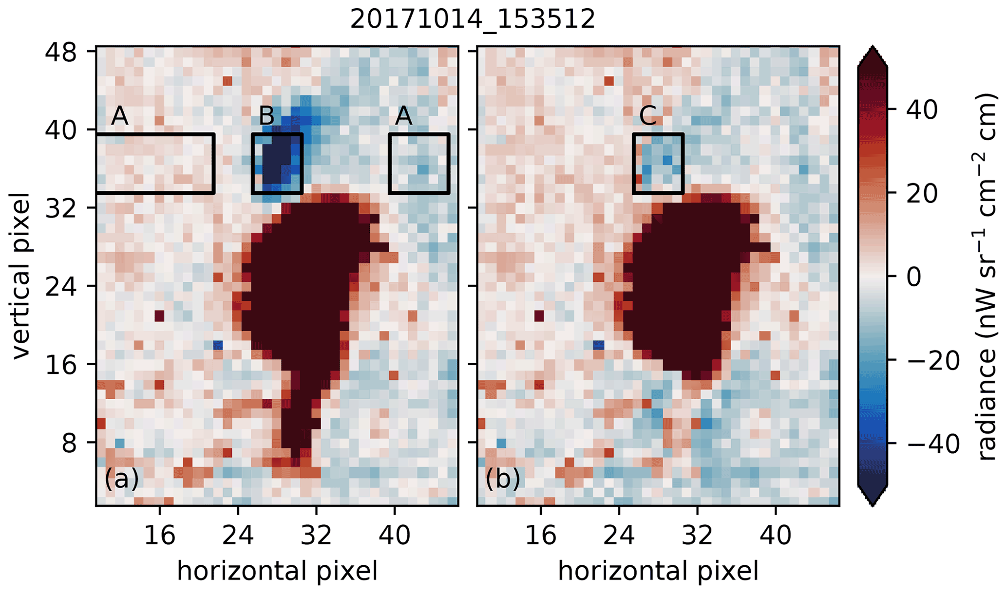
Figure 8 Panel (a) shows the average radiance of a moon image from 14 October 2017; note the two strong parasitic images above and below. Panel (b) shows the same image after parasitic image correction was applied. The same background was subtracted from both images, and was computed for each row individually from the median over all pixels outside the columns containing moon-affected pixels. The black rectangles indicate regions related to the spectra shown in Fig. 9.

The correction vector contains the positions (in whole pixels) and the magnitudes of the upper and lower parasitic images. These four free parameters were determined from six independent moon measurements taken during three separate flights and located at various locations on the detector. The parameters were varied manually until we got a satisfactory correction for all six measurements. We found a common shift of the parasitic images of 16 pixels and a factor of 1.8±0.2 % for the negative upper image and $-\mathrm{2.5}\pm \mathrm{0.2}$ % for the positive lower image. The errors were estimated from the range of visually acceptable values.

Figure 8b shows the corrected image. One can see some remaining small artifacts that could not be fully removed by tuning the four parameters; we believe this to be caused by our overly simple and discrete model of the effect.

To properly quantify the remaining effect after correction, we inspected spectra averaged over the three regions indicated in Fig. 8. The three spectra represent (A) the background of the atmosphere outside the region affected by the parasitic image of the moon, (B) the spectra most heavily affected by the negative parasitic image, and (C) the corrected version. Figure 9a shows the three spectra. Spectrum B is generally decreased outside the 1000 cm⁻¹ region, where the radiance field is vertically homogeneous due to strong ozone emissions. The difference plot of the affected spectrum (B–A) shown in Fig. 9b points to a discrepancy of up to ≈100 nW cm⁻² sr⁻¹ cm. The corrected spectrum (C–A) does not exhibit obvious defects above the NESR level.

Figure 9 Panel (a): spectra averaged over all pixels marked by black rectangles in Fig. 8. “A” refers to all pixels in the two outer rectangles in Fig. 8a, whereas “B” refers to all pixels within the center rectangle. “C” refers to all pixels in the center rectangle of Fig. 8b. (The “A” and “C” spectra are very similar.) Panel (b) highlights the differences between the spectra shown in panel (a).

The effect is worst at cloud tops, where the radiance can quickly drop from >5000 nW cm⁻² sr⁻¹ cm to <500 nW cm⁻² sr⁻¹ cm over a couple of pixels. Underestimations of up to 100 nW cm⁻² sr⁻¹ cm above cloud tops were observed in a couple of profiles. With the assumed uncertainty, the effect is reduced by an order of magnitude to ≈10 nW cm⁻² sr⁻¹ cm in the worst case (close to cloud tops), but typically remains below the noise level.

4.5 Bad pixel identification

The behavior of individual pixels of the detector of GLORIA changes significantly from flight to flight to the extent that we need to determine a separate list of bad pixels for each flight. These pixels are then excluded from horizontal averaging when preparing the final level 1 products. The classification into “good” and “bad” pixels is always somewhat arbitrary, and there are a considerable number of pixels that do not unambiguously belong in either category. The goal of our bad pixel identification is to identify and discard only the worst pixels that would affect the level 1 product when included. We define good pixels as pixels that agree with the median value of their row. To exclude the effects of inhomogeneous scenery on the one hand and use measurements closely resembling regular atmospheric measurements on the other hand, we decided to analyze the deep space measurements, which are cloud free and available in sufficient quantities for all flights.

For each pixel and deep space measurement, we compute the root mean square error (RMS) between its value and the median of the row over all spectral samples. Analyzing each flight individually, we can examine the histograms of the RMS values computed in this manner, which always show a very similar structure (Fig. 10): a Gaussian-like peak that slowly trails off at high values. This is due to the behavior of “standard” pixels with a Gaussian noise distribution on the one hand and the influence of other pixels with increased noise or other erratic behavior on the other hand. The general noise level and spread varies from flight to flight and from campaign to campaign due to differences in the configuration, electronics, and detectors employed. We assume that the left side of the distribution in Fig. 10 closely resembles the Gaussian distribution of “good” pixels and fit a Gaussian function with an unknown mean, standard deviation, and scaling to it. About 4 % of the pixels are beyond the limits of the plot. The Gaussian curve fits reasonably well to the left-hand side of the distribution and the peak. We then define the pixels for which the median of the difference computed over all deep space measurements is larger than the mean plus 9 times the standard deviation as the bad pixels. We use the median here as defects in the calibration offset of a single calibration sequence could otherwise cause a large number of pixels to be discarded. Figure 11 shows the masks derived using different thresholds. The 9σ threshold is by design very inclusive, and the probability of excluding good pixels is negligible, as we are not interested in discarding a pixel solely for displaying a slightly increased amount of noise. Still, we find that ≈10 % of the detector pixels are excluded by this criterion on average. About half of these excluded pixels are obviously defective; these are mostly found in the outermost columns, where the read-out electronics has known issues. The other half show a variety of behaviors; for example, some pixels exhibit a telegraph noise pattern, switching their mean values rapidly between different levels, while others vary in their nonlinearity during the flight and thus have an offset during longer periods of time.

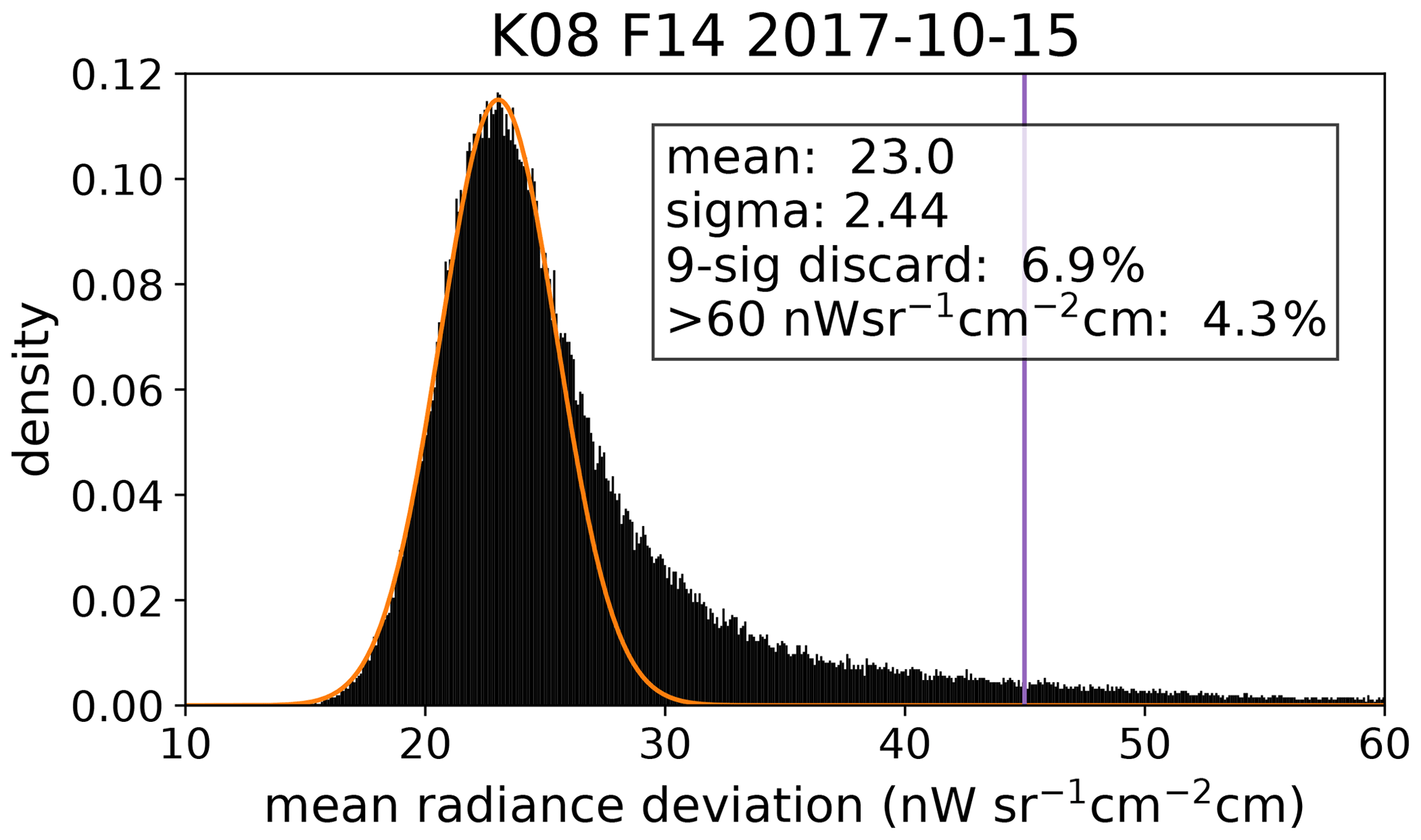
Figure 10 Distribution of spectrally averaged absolute differences from the horizontal median value for the 14th flight of the WISE campaign. A Gaussian curve (orange) is fitted to the left hand side of the distribution. The vertical bar (purple) shows the chosen 9σ threshold. 4.3 % of all values lie outside this plot.

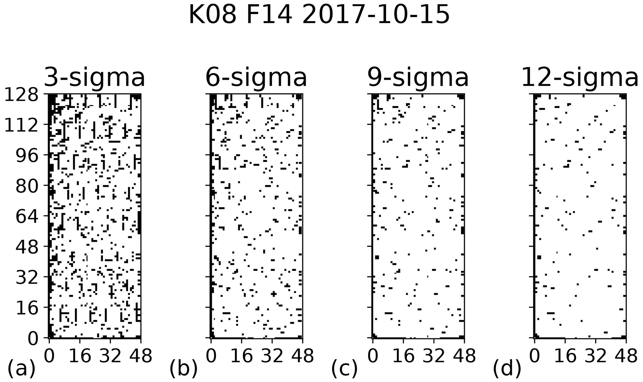
Figure 11 Different bad-pixel masks for the 14th flight of the WISE campaign. Bad pixels are colored black. Panel (a): for a 3σ threshold (19.0 % filtered). Panel (b): for a 6σ threshold (10.4 % filtered). Panel (c): for a 9σ threshold (6.9 % filtered). Panel (d): for a 12σ threshold (5.2 % filtered).

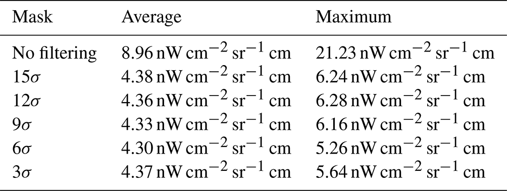
Figure 11c shows the mask that was finally chosen for an example flight. In Fig. 11a, a mask with a stricter 3σ threshold is shown for comparison. This mask shows large clusters of masked pixels in the top left corner, which are likely to have been flagged due to border effects in the smoothing of the calibration offset. For reference, a more relaxed 12σ threshold is also depicted in Fig. 11d. To obtain further support for the chosen threshold, we also examine both the noise of the level 1 data and the quality of the level 2 results (trace gases and temperature). All depicted masks perform very well with respect to the level 2 results, whereas applying no mask causes artificial horizontal structures in the level 2 data. Estimating the average noise of spectral samples of cloud-free pixels gives us Table 3. Employing no filtering increases the average noise value significantly. All thresholds effectively filter out really bad pixels to the extent that the estimated noise is very similar. Due to the irregular distribution of more noisy pixels on the detector, using a strict threshold can decrease the number of remaining pixels in some rows to only a handful, causing the average noise value to increase again. To make the most of the available measurements, we thus decided to use the 9σ threshold.

Table 3 Average noise value of a 0.625 cm⁻¹ spectral sample and maximum noise of a superpixel averaged over all 0.625 cm⁻¹ spectral samples for different bad-pixel masks. The smaller the n in nσ, the more the pixels will be filtered.

4.6 Pointing analysis

GLORIA makes use of a highly sophisticated and precise pointing system based on high-precision sensors and a gimbal mount allowing adjustment along all three axes. The pointing system enables two different limb view acquisition modes for high spatial and high spectral resolution, nadir pointing, as well as calibration. Different control modes are connected to these observation scenarios because they have different requirements. The major features of the different control modes and the pointing system are described in Appendix C.

An additional camera operating in the visible spectral domain is mounted on the interferometer. This camera covers a wide field of view (FOV), thereby completely enclosing the FOV of the spectrometer. For most of the interferograms, correlated images of the scene or video sequences are taken. The information provided by this camera can be used for cloud identification and for pointing quality analysis.

Limb sounding and the associated retrieval depend strongly on the acquisition and absolute knowledge of the line of sight. Therefore, an on-ground calibration is needed to determine pointing offsets and to achieve good pointing acquisition in flight. For this purpose, we have built a calibration optics system that delivers parallel beams with a broadband infrared light source and an off-axis parabolic mirror. Since this optical system is made for several purposes, such as determining FOV and adjusting the focal length of the spectrometer, there are five sources arranged like the five on a die, but only the source in the middle is used for the pointing calibration. The sources can be seen in both the visible and the infrared spectral ranges. The calibration optics are mounted on a tripod, and the beam from the middle light source is adjusted with the help of a theodolite to be horizontal with an accuracy of ≈0.05 mrad. This optical system, which is placed in front of the instrument and points towards the spectrometer, allows for the determination of the offset angle between the nominal horizon of the gimbal control and the real horizon (see Fig. 12). This offset value is passed to the control system so that the output measured elevation is referenced to the real horizon. The image of the source on the GLORIA detector has a size of 3–5 pixels (see Fig. 13). We assume an uncertainty of 1 pixel when determining its center, which corresponds to ≈0.03^∘.

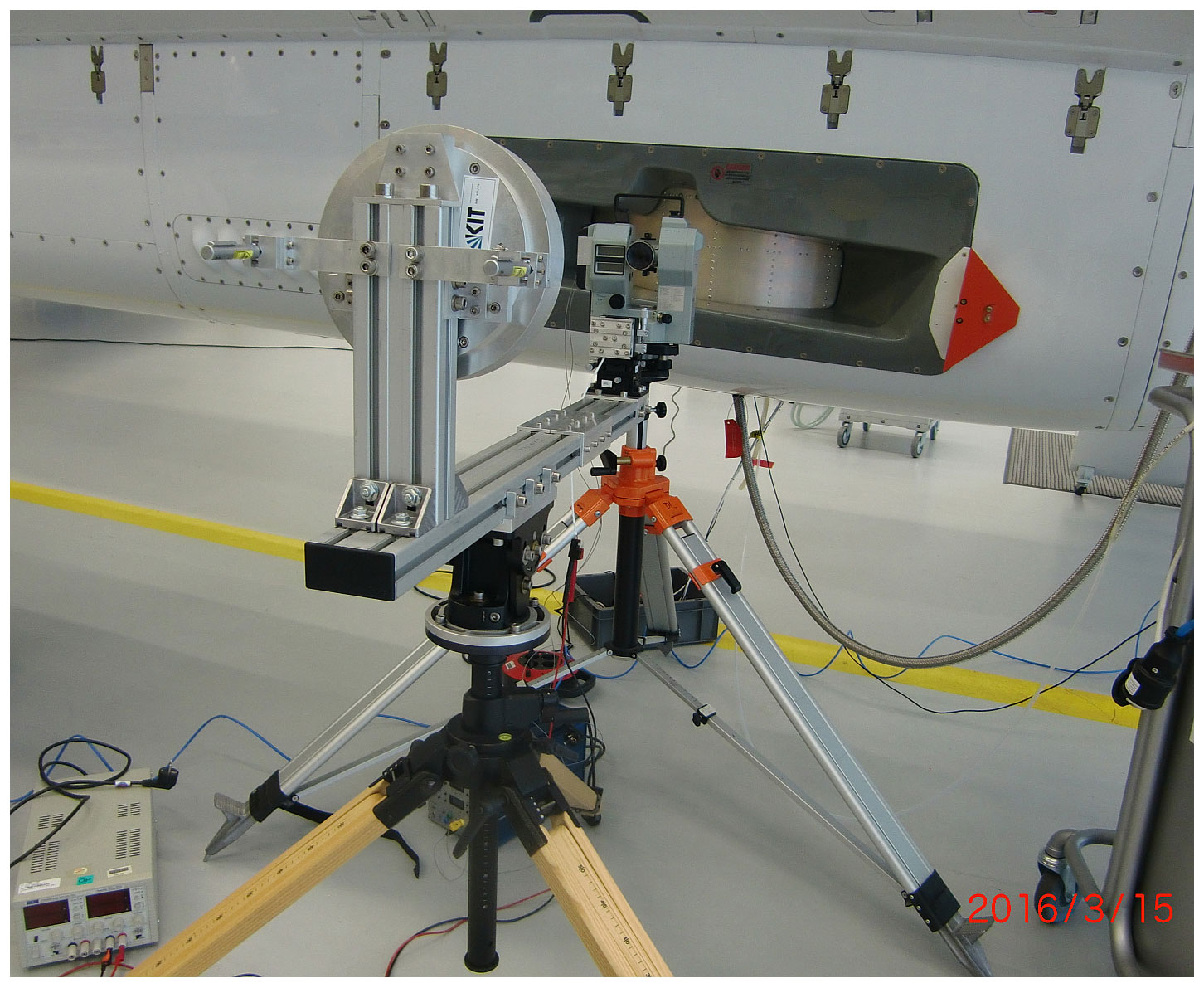
Figure 12 Pointing calibration optics with an off-axis paraboloid mirror that delivers parallel beams from a broadband infrared light source to the GLORIA instrument (gold-colored) integrated into the belly pod of HALO in Oberpfaffenhofen. During the beam adjustment phase, the theodolite is located between the pointing calibration optics and GLORIA.

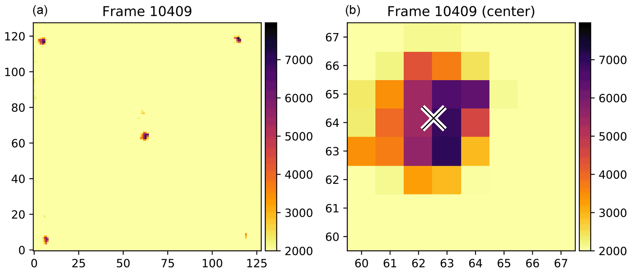
Figure 13 Measurements of the five light sources delivered by the pointing calibration optics. Panel (a) shows the full detector, which was read out with 128×128 pixels for this measurement. Panel (b) shows a close-up of the central beam that highlights the 0^∘ pitch/90^∘ azimuth position.

With the equipment described above, this measurement can be taken for any elevation value. However, azimuth calibration is more difficult. The best azimuth calibration is performed in the base hangar for HALO at DLR (Deutsches Zentrum für Luft- und Raumfahrt). In this hangar, TU Dresden measured the precise coordinates of reference points marked on the hangar walls and also on the floor close to the position of the integrated GLORIA (Scheinert and Barthelmes, 2014). Using these marks, it is possible to validate the absolute azimuth and elevation with respect to the pointing system of GLORIA. In the laboratory at KIT (Karlsruhe Institute of Technology), there are known positions of some landmarks, so the azimuth can be determined there as well, but not as accurately as in the hangar at DLR. We thus assume a higher uncertainty in azimuth of ≈0.1^∘.

Due to the high demands of limb sounding, it is necessary to determine the absolute pointing in flight. The on-ground calibration has to be verified and corrected because the absolute pointing of the instrument typically changes between ground and flight conditions due to thermal warping. This absolute attitude might also change from flight to flight during a campaign, for instance due to the forces that act on GLORIA during the landing of the aircraft. Sometimes, misconfiguration of the instrument or exchanging the navigation system for the spare has a similar effect.

In order to perform an in-flight LOS calibration, a suitable astronomical object has to be observable by GLORIA, i.e., close to the horizon and on the right side of HALO. During WISE, several dedicated observations of moonrise and moonset were made, which provided an absolute calibration source under flight conditions. Since the flight time and path of the aircraft were determined by the scientific goals of the flight, such measurements were only feasible as secondary objectives during three flights of the WISE campaign. One such measurement is shown in Fig. 14. Refraction of visible light close to the horizon impacts the apparent position of the moon. Our approach to correcting for this is described in Appendix D. Since the WISE campaign in 2017, we have made moon calibrations whenever feasible. For earlier campaigns, an analysis of our measurements revealed some accidental moon measurements. The visible camera can easily locate Venus and other planets visible to the naked eye, but the derived LOS from such measurements comes with the added uncertainty in the alignment between the visible and IR cameras. In the infrared, the planets are much less bright, but we successfully identified Venus after averaging 48 images, thus providing an alternate target for line-of-sight calibration.

Figure 14 Example of the determination of the position of the moon for one cube measured on 14 October 2017 at 15:37:58 Z. Panel (a) shows the full image, while panel (b) shows the moon in an enlarged fashion. The expected position of the moon is shown in blue; the manually determined actual one is in orange. Here, the difference between the expected and actual positions of the moon is 0.78^∘ horizontally and 0.2^∘ vertically.

In addition to these direct but sparse pointing measurements, we perform level 2 retrievals to determine the attitude. Here, we use data from two such retrievals: one based on data acquired with high spectral sampling (0.0625 cm⁻¹; Johansson et al., 2018) and one based on data acquired with intermediate spectral sampling (0.2 cm⁻¹; see Appendix F for details), which is available for all profiles. For campaigns prior to 2017, only data with coarse spectral resolution (0.625 cm⁻¹) are available for some flights. For those flights, a different approach based on the retrieval described by Ungermann et al. (2015) was used, where an elevation correction value was derived instead of temperature (the CO₂ lines used from WISE onwards are not sufficiently resolved in the early campaigns). We typically use only a single correction factor for a flight; this factor is determined after filtering short (less than 3 km between the instrument and cloud top) profiles from the mean of the remaining values. An error estimate is computed from the standard deviation.

All line-of-sight characterizations for the WISE campaign are aggregated in Fig. 15. The attitude was calibrated using on-ground calibration before and after the campaign. Between WISE flights 2 and 3, the inertial navigation system had to be exchanged for the spare, causing a change in elevation offset. Between flights 13 and 14, the pointing was readjusted using information from preliminary level 2 and moon data that suggested a systematic offset of 0.17^∘ at the time. Thus, the pre-campaign calibration is applied to flights 1 and 2 and the results of the post-campaign calibration are applied to the remaining flights. The values of the different level 2 retrievals agree within the respective error bars. In this particular campaign, the moon calibration seems to indicate a systematically smaller elevation correction, but other campaigns also show higher values. The differences between the various methods and calibrations are consistent within the estimated uncertainties. For further processing, we typically select the most reliable value (depending on the number of available profiles and the spectral resolution) from the level 2 result. For the remaining error, we assume simply an uncertainty of 1 pixel, i.e., ≈0.032^∘.

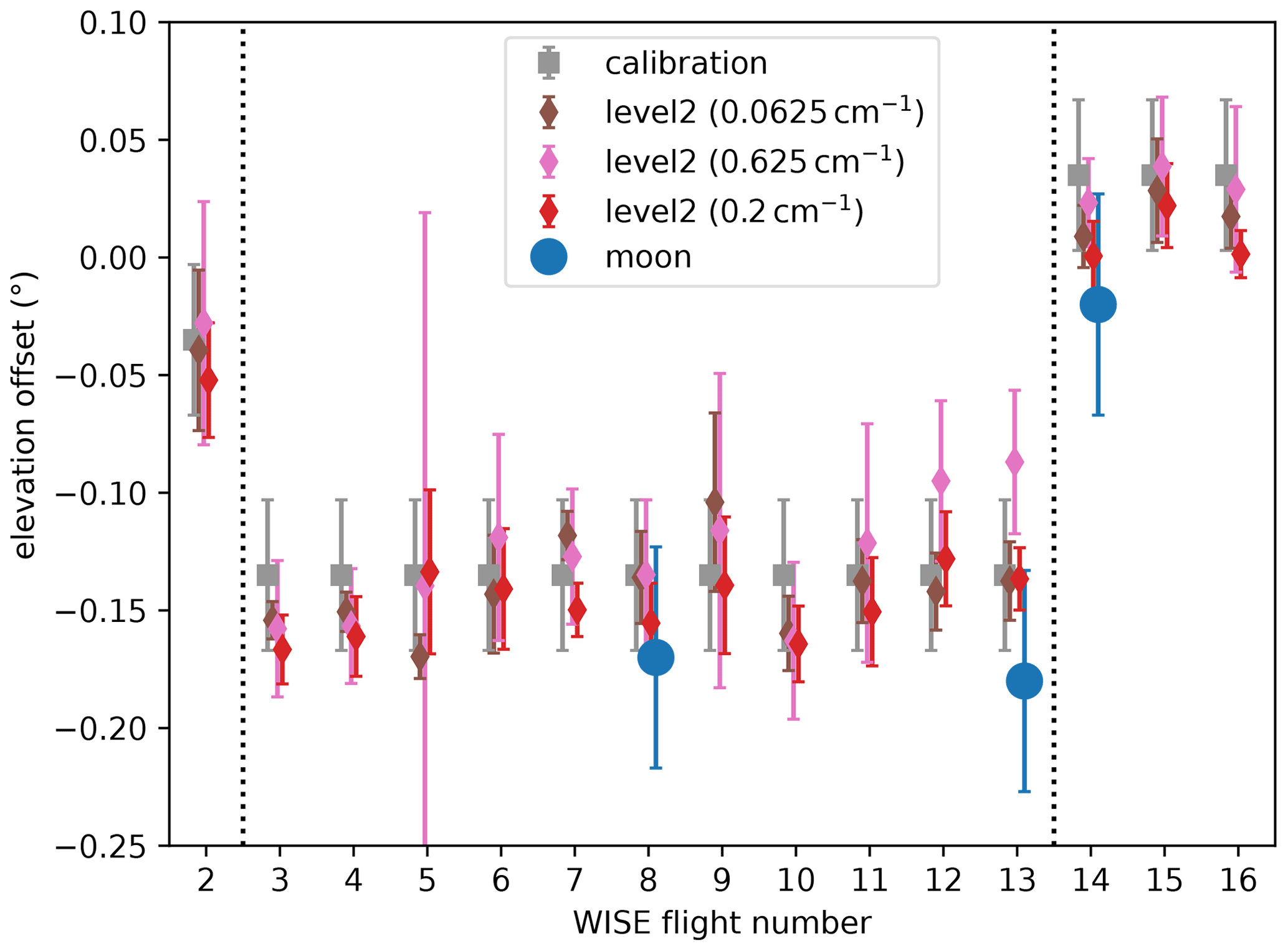
Figure 15 Values derived for the absolute elevation offset during the WISE campaign. Blue circles are offsets determined from moon measurements, while gray squares are values derived from calibration measurements taken pre- and post-campaign (pre-campaign for the first two flights, post-campaign for the remaining flights). Pink, red, and brown symbols are elevation angles determined from level 2 processing and ECMWF temperature data. The leftmost dotted line marks the point at which the inertial navigation system was changed, which invalidated the attitude calibration. The rightmost dotted line marks the point at which the employed elevation angle offset correction was changed, with the pointing corrected according to the best level 2 data at that time.

5 Performance and characterization

This section gives an analysis of the quality of our level 1 data from in-flight data and aggregates the (simplified) results in a table to serve as the basis for error estimates of level 2 products such as temperature and trace gas VMRs.

5.1 Noise equivalent spectral radiance (NESR)

Friedl-Vallon et al. (2014) estimated the NESR of GLORIA from selected measurements to check that it was within specification. Here, we extend that work to estimate the noise of individual atmospheric measurements taken at different altitudes and on different flights. For the level 2 processing, we need to determine the NESR associated with spectra averaged over an entire row. We thus focus on the NESR of spectra averaged over the detector rows.

Several methods can be used to estimate the NESR from measured spectra. In an ideal instrument, the imaginary part of the calibrated spectrum contains only measurement noise. In practice, however, it also contains some residual signal due to, e.g., small phase errors (the effect of which is negligible in the real part of the spectrum), asymmetries in the interferogram due to a variable scene (especially in the presence of clouds), and artifacts introduced by calibration inaccuracies in the imaginary part of the instrument offset. Instead, we use two different methods to determine the NESR from the real part of the spectrum.

In the first method, we look for each detector pixel at the radiance variation over seven consecutive measurements of a deep space sequence. We can safely assume that the observed scene stayed constant during this brief time frame. These pixel-based estimates are used to determine the NESR of horizontally averaged values using the bad-pixel mask determined in Sect. 4.5. Then, the resulting NESR spectra are averaged vertically to present a single spectrum.

In the second method, we only use a single deep space measurement, and we look at the horizontal variation from detector pixel to detector pixel. In particular, the NESR is estimated by computing the horizontal standard deviation (again excluding bad pixels, as determined according to Sect. 4.5) for the first measurement of the sequence only. These values are then divided by the square root of the number of corresponding valid horizontal pixels and averaged as above over the vertical dimension.

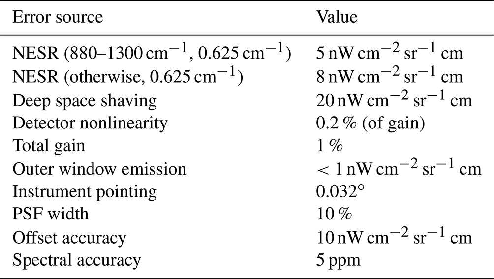
Results from both methods plotted against wavenumber are compared in Fig. 16. These noise spectra were computed for deep space measurements processed at the full (0.0625 cm⁻¹) spectral resolution of the high spectral resolution mode as well as the reduced (0.625 cm⁻¹) spectral resolution of the high spatial resolution mode, which we also use for blackbody measurements. The NESR spectra derived from horizontal variation are 10 % and 5 % higher than those derived from temporal variation. This is partially expected, as calibration noise and calibration inaccuracies only contribute in the horizontal variation analysis. We also observe additional structures in the ozone 1000 cm⁻¹ band, which we associate with imperfections in the shaving. Locally enhanced values in the NESR are caused by electrical disturbances. The highly resolved NESR spectra are 3.14 and 3.03 times higher than those derived from low-resolution data for the temporal and horizontal variation methods, respectively. This is reasonably close to the expected factor of $\sqrt{\mathrm{10}}$, meaning that the NESR can be estimated from measurements with either resolution and scaled to any other resolution employed in atmospheric observations.

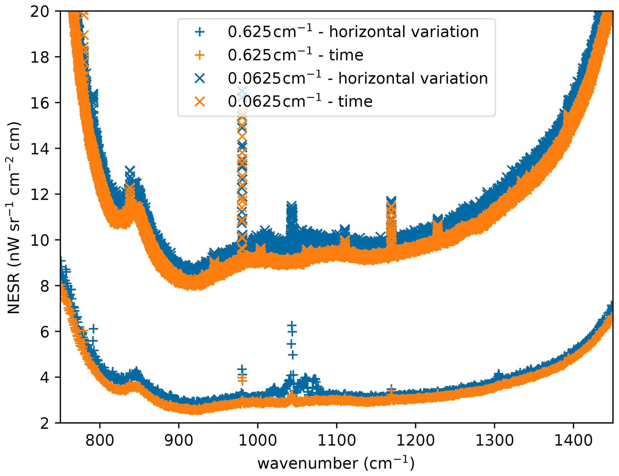
Figure 16 Examples of NESR estimates from a sequence of deep space measurements processed at two different spectral resolutions and using two different methods.

Employing the second method, we can now produce a NESR estimate for all of our atmospheric measurements, allowing us to closely track instrument performance over the whole flight. Figure 17 shows an example of such an analysis for a set of roughly 200 evenly distributed measurements from one flight. Figure 17a depicts an averaged NESR spectrum; only spectra determined as fully cloud free (i.e., with a cloud index of more than 6 according to Spang et al., 2012) are included in this average. Figure 17b shows the evolution of noise over time as a pseudocolor plot. The NESR is spectrally averaged in the range from 750 cm⁻¹ to 1450 cm⁻¹. The beginning of the flight before 14:00 Z shows increased NESR values, which can be attributed to the higher blackbody and outer-window temperatures. The higher blackbody temperatures at the beginning of the flight require a shorter integration time for calibration measurements, which are thus subject to a higher NESR, affecting the calibration quality. The high values in the lower part of the detector array are due to clouds, which lead to spatial inhomogeneities and thus to overestimation of the NESR. The last panel (Fig. 17c) shows the noise of individual rows averaged over cloud-free measurements. The lowermost rows are missing since no cloud-free spectra were available for analysis. Some high values due to unidentified small-scale clouds remain in the lowermost rows with data. At higher altitudes, one can see that the NESR is not uniform over all rows due to the readout electronics and the uneven distribution of filtered pixels. Typically, all flights of a campaign exhibit very similar NESR characteristics, but we can observe small variations from campaign to campaign, such as a generally increased NESR value due to changes to the instrument or its operation parameters.

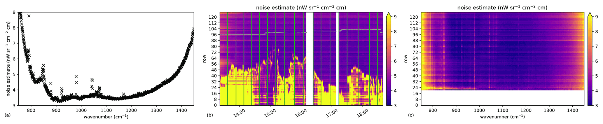
Figure 17 Example of the NESR analysis of atmospheric spectra for the WISE flight of 15 October 2017. Panel (a) shows a single NESR spectrum averaged over time and pixels. Panel (b) shows the spectrally averaged NESR. Panel (c) shows the NESR averaged over time.

From this and an analysis of other flights, we derive typical values of the NESR: 5 nW cm⁻² sr⁻¹ cm for the wavenumber range between 880 and 1300 cm⁻¹ and 8 nW cm⁻² sr⁻¹ cm outside this range for a spectral resolution of 0.625 cm⁻¹. The NESR scales up by a factor of $\sqrt{\mathrm{3.125}}$ for a spectral resolution of 0.2 cm⁻¹ and by a factor of $\sqrt{\mathrm{10}}$ for a spectral resolution of 0.0625 cm⁻¹ (see Table 4).

Table 4 Simplified estimates for the examined error sources.

5.2 Gain accuracy

This section estimates the stability of the gain magnitude from in-flight data. During the calibration, we compute a gain magnitude for each calibration sequence containing a pair of blackbody and deep space measurements, each of which gives an independent gain estimate (see Sect. 3). These estimates are averaged in a subsequent step to reduce the impact of measurement noise. The variability of these gain magnitudes gives us an uncertainty estimate upon computing the standard deviation of the gain magnitude for all flights and all pixels. The median standard deviation over all pixels is shown in Fig. 18 for several flights of the WISE campaign. The resulting accuracy is better than 0.1 % and thus well within our target range of 1 %. One can see an increased uncertainty towards the edges of the usable wavenumber range; this is caused by the decreased sensitivity of the detector, which corresponds to a lower SNR. Towards lower wavenumber regions, one can also see a spectral structure that resembles the window emission feature shown in Fig. 6; these are likely caused by small temperature variations of the window during the rather long deep space measurements. Increased uncertainty at the locations of strong ozone and methane emissions at around 1050 and 1300 cm⁻¹ can also be observed, which is most probably due to imperfections in the shaving of deep space spectra. While these estimates show the average uncertainty of a single detector pixel, we also use them to describe the accuracy of horizontally averaged data because some of the underlying errors are strongly correlated (such as the impact of atmospheric window emissions). We pick the highest uncertainty among all the flights to use it as the worst-case assumption (maximum) for analysis.

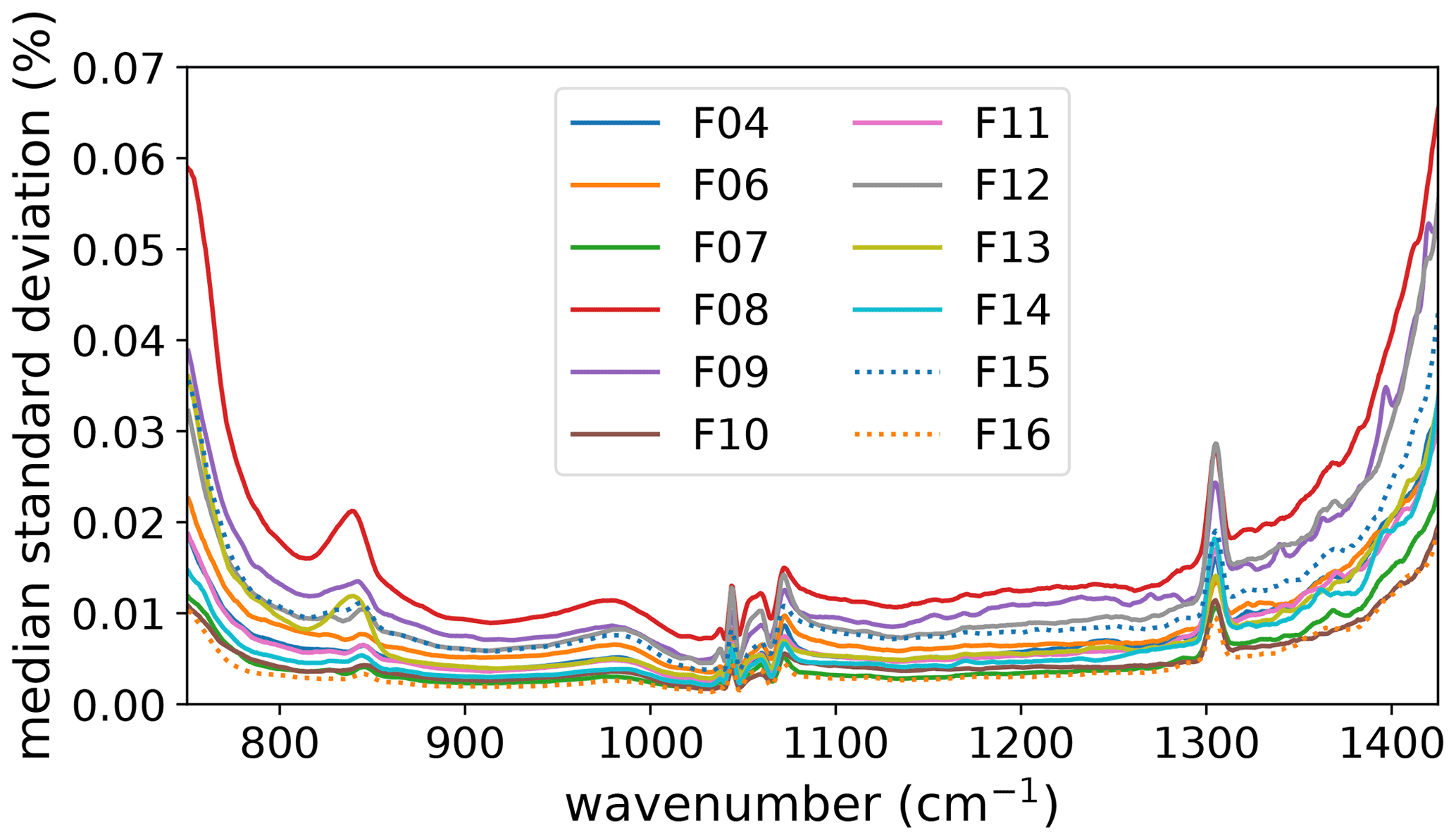
Figure 18 Uncertainty in gain magnitude. The plot depicts the standard deviation computed over the individual gain magnitudes from all calibration times of the given flights in the WISE campaign.

In addition to these variations, our gain might be subject to a systematic error common to all measurements. There are a range of potential sources of such a systematic error; for example, inaccurate blackbody temperatures, uncorrected detector nonlinearity, or shaving defects. To gain an independent estimate of the absolute accuracy of the gain magnitude, we turn to atmospheric measurements and compare the calibrated spectra with the Planck curve of ambient temperature in a wavenumber range located within the optically thick ozone Q-branch from 1050 to 1056 cm⁻¹. We select only the atmospheric profiles for which the ECMWF indicates that the ozone VMR was above 300 nmol mol⁻¹ to ensure sufficient optical thickness and thus practically no dependence on the actual ozone VMRs. Computing the relative difference between the calibrated measurements and the Planck curve indicated by ECMWF temperatures for 3000 WISE profiles yields an average difference of 0.1±2.0 %. This rather high uncertainty is caused by small-scale temperature perturbations not present in ECMWF data at the employed resolution ($\mathrm{1}{}^{\circ }\times \mathrm{1}{}^{\circ }$). A similar analysis for other campaigns gave slightly larger differences. For SouthTRAC data, a difference of $-\mathrm{0.9}\pm \mathrm{2.5}$ % was identified, and for PGS, a difference of $-\mathrm{1.3}\pm \mathrm{2.6}$ %. In all cases, we could not reject the null hypothesis that there is no gain bias in GLORIA data. As both the offset and gain errors are reflected in this analysis as well as the inherent uncertainty in ECMWF temperatures, it is difficult to quantify exactly how accurate the gain is. Instead, we can give an upper bound of 2 %, which fits well to our threshold requirement (Friedl-Vallon et al., 2014). For level 2 error estimates, we assume a general gain magnitude error of 1 %, which obviously may imply higher or lower errors for individual flights.

5.3 Offset accuracy

The instrument gain and offset are determined using a direct measurement of the deep space background. Thus, we expect only small, correlated errors due to measurement noise and imperfect shaving of atmospheric contributions.

In order to quantify these errors in the offset, we analyzed special in-flight measurements where the elevation angle of the optical axis of GLORIA alternated between −0.38 and −1.00^∘ for 12 consecutive images. We interpolated each profile to an evenly spaced elevation axis, computed differences between successive measurements, and finally averaged the differences. The results are depicted in Fig. 19. Within the overlapping range, we find a difference of $-\mathrm{1.7}\pm \mathrm{5.3}$ nW cm⁻² sr⁻¹ cm between the different pitch angles. Although not statistically significant, the higher-pointing measurements are colder, which would be consistent with an influence of warm stray light from below on the measurements. The available measurements do not allow for a full quantification of the effect, though. Analyzing the discrepancies in more detail reveals spectrally and spatially correlated structures with magnitudes of up to 6 nW cm⁻² sr⁻¹ cm above 900 cm⁻¹ and magnitudes reaching towards 16 nW cm⁻² sr⁻¹ cm below 900 cm⁻¹ (Fig. 19b). The differences observed around 1000 cm⁻¹ and other strong emission features may be partially caused by errors in the gain, not the offset. The magnitude of the difference is similar for both upwards-pointing and downwards-pointing pixels. This lends weight to the hypothesis that it is largely caused by an offset error, as the measured radiances are much higher at lower pixels, which would lead to higher absolute differences in the case of gain errors. Due to the various smoothing methods employed to generate the offset calibration data, we also expect both spatial and spectral correlations. We assume here a correlation length estimated by eye of 10 pixels vertically and 50 cm⁻¹ spectrally, and average the magnitude to 10 nW cm⁻² sr⁻¹ cm. This error is separate from the systematic uncertainty from shaving.

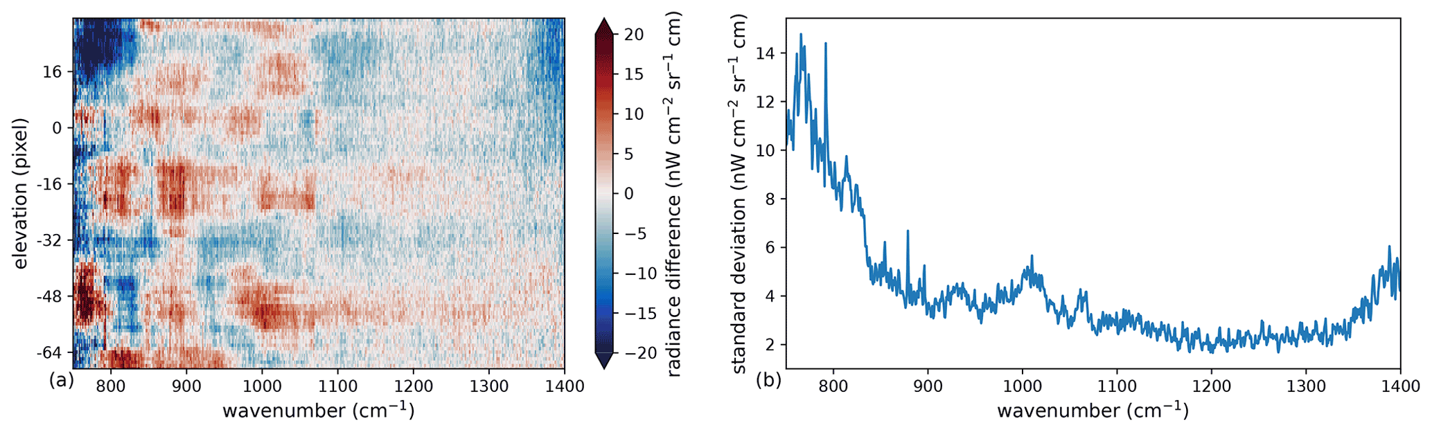
Figure 19 (a) Difference in calibrated radiance when measuring the same air mass at two different elevation angles and (b) the standard deviations thereof. The measurements were taken during the POLSTRACC campaign on 2 February 2016 at 22:00 Z, alternating between −0.38 and −1.00^∘ elevation.

5.4 Spectral accuracy

The spectral axis of our level 1 data depends on the proper association between the taken images and the optical path difference. We perform an off-axis correction and characterize the laser wavelength as described by Kleinert et al. (2014), using the deep space measurements. These are cloud free and taken periodically in high spectral resolution mode.

While the geometric parameters, which determine the off-axis angle, stay constant during each flight, we found that the laser wavelength sometimes varies significantly, e.g., because of temperature drifts and the resulting laser mode hops. In order to obtain better temporal resolution of the evolution of the laser wavelength, we modified our spectral calibration algorithm to determine only the laser wavelength from otherwise off-axis corrected calibrated atmospheric spectra. This allows us to do quality checks on calibrated and horizontally averaged level 1 data and to better quantify our uncertainty. For each atmospheric measurement, all pixels unaffected by clouds are averaged, and the resulting spectrum is analyzed for a spectral shift. Due to the high SNR, this spectrum also allows reliable spectral shift determination from data measured with decreased spectral resolution. This enables continuous monitoring of the laser wavelength over the flight, as many atmospheric measurements are available only at 0.625 or 0.2 cm⁻¹ resolution. The method involves locating the positions of CO₂ emission lines in the 950 cm⁻¹ wavenumber region and comparing them with the expected line positions in the HITRAN database (Gordon et al., 2017). Estimating the spectral accuracy of 0.625 cm⁻¹ spectra requires a dedicated processing run using a Norton–Beer weak apodization instead of the usually employed Norton–Beer strong apodization (Norton and Beer, 1976, 1977).

Figure 20 shows the resulting spectral shifts for an example flight of the WISE campaign. The most precise results are from spectra of the highest spectral resolution. The spectra with 0.2 cm resolution have a larger spread, whereas the 0.625 cm⁻¹ spectra have large errors of about 5–10 ppm (i.e., a relative error in wavenumber knowledge of less than 0.001 %), and are thus only useful for a qualitative analysis (to detect large errors). For this flight, the spectral accuracy is of the order of 1 ppm on average. Using the 0.2 cm data, the accuracy is still diagnosed to be better than 2 ppm. This is much better than the original target accuracy of 10 ppm. Applying this technique to all flights of the WISE campaign, we estimate the spectral accuracy to be of the order of 2 ppm. The same accuracy is also valid for other campaigns from PGS onward, with the exception of a few flights that are subject to known technical issues. To account for additional variations over the detector, and to include outliers, we use an accuracy estimate of 5 ppm (see Table 4). This corresponds to about one-tenth of the smallest employed spectral sampling distance of 0.0625 cm⁻¹ at the largest wavenumber of 1400 cm⁻¹.

Figure 20 Example of the spectral shift analysis of atmospheric spectra for the WISE flight of 15 October 2017. The shifts derived from atmospheric measurements processed at different spectral resolutions are depicted.

5.5 Point spread function

The point spread function (PSF) determines the amount and direction of the incoming light measured by the detector pixels. The theoretical shape for a diffraction-limited instrument, such as GLORIA under nominal operation conditions, is the Airy disk:

$${\displaystyle }\begin{array}{ll}a\left(r\right)={\left(\frac{\mathrm{2}{J}_{\mathrm{1}}\left(\mathit{\nu }Dr\right)}{\mathit{\nu }Dr}\right)}^{\mathrm{2}}& \text{for}r>\mathrm{0},\\ a\left(r\right)=\mathrm{1}& \text{for}r=\mathrm{0},\end{array}$$

where J₁ is the Bessel function of the first kind, ν is the wavenumber, D is the aperture, and r is the distance to the optical axis.

This function defines the PSF for a pixel of infinitesimal extent, and needs to be integrated over the pixel size to determine the actual PSF for the pixel. In the horizontal direction, because of our averaging over full rows, we can assume an effectively infinite extent with only a small error, but in the vertical direction the detector pixel width needs to be considered.

The optical aperture diameter is 3.6 cm. Figure 21 shows several PSF functions for apertures of 3.2, 3.6, and 4.0 cm in the upper panel. The lower panel demonstrates how the PSF changes with wavenumber.

Figure 21 The impacts of (a) the aperture and (b) the wavenumber on the theoretical point spread function.

We verify that this theoretical PSF shape is consistent with the results of the in-flight measurements and use it to estimate how an error in the PSF knowledge affects the retrieval quality. The PSF was previously verified with laboratory measurements, which showed that the instrument response is consistent with a diffraction-limited optical system.

We examine the PSF using extinction values from level 2 retrieval results. In the presence of optically thick cloud tops, artifacts appear in the retrieved extinction values if the simulated PSF is different from the real one. With a PSF that is too wide, the modeled radiance above the cloud top is overestimated and, accordingly, unnaturally small extinction values are generated in order to properly simulate the measured radiances. With a PSF that is too narrow, there is no expected sharp step in the extinction profile at the cloud top; there is a more gradual increase in the transition region instead. This is exemplified by the extinction profiles shown in Fig. 22, which were retrieved with different aperture sizes based on the retrieval approach discussed by Ungermann et al. (2020). For a PSF with an assumed aperture smaller than 3.6 cm, the extinction even drops below the background values found at higher altitude values above the cloud top. For this specific profile, a sensible extinction profile can only be derived with an aperture of at least 3.6 cm. While the range of admissible apertures varies from profile to profile, all derived extinction profiles were plausible for an aperture of 3.6 cm. The same experiment was performed at a different atmospheric window at 1214 cm⁻¹. This showed similar results for the corresponding PSF, so the retrieval results are consistent with the expected values from instrument design. Based on the different characterization methods and the variability of the results, we assume an uncertainty of 10 % in the width of the PSF.

Figure 22 Examples of extinction profiles derived using point spread functions with differing apertures.

6 Analysis of the impact on level 2 data

The comprehensive characterization of leading level 1 errors from in-flight data is a solid basis to revisit our level 2 results and estimate the impact of these errors on our derived quantities.

The retrieval of geolocated physical quantities from limb measurements is a ill-posed nonlinear problem. Using a forward model simulating the radiative transfer, one adjusts geophysical quantities such as temperature or trace gas VMRs until the simulated radiances agree with the measured ones within expectation (e.g., Rodgers, 2000). For efficiency, we typically apply a linearized Gaussian error analysis after deriving an atmospheric profile (e.g., Ungermann et al., 2015; Johansson et al., 2020). Here we use a simpler approach to also allow for the quantification of all errors estimated in this paper, including those for which the forward model does not offer the necessary derivatives.

For brevity, we examine only two quantities. We selected temperature as it is the fundamental quantity necessary for all further retrievals, and we selected ozone as it is one of the most commonly retrieved trace gases. The corresponding retrieval setups are described in Appendix F. We assumed here that the given errors, with exception of the NESR, are systematic and affect all measurements taken during one flight in the same way. We picked flight 10 (7 October 2017) of the WISE campaign for this exercise as it offers many profiles reaching deep into the troposphere.

• To examine the effect of NESR, we applied an independent Gaussian noise of 14.4 nW cm⁻² sr⁻¹ cm to all samples (the employed spectral resolution of the level 1 data was 0.2 cm⁻¹).

• The effect of the deep space shaving error was estimated by adding 20 nW cm⁻² sr⁻¹ cm to all measurements.

• The effect of the detector nonlinearity was estimated by generating a Gaussian distributed gain error with mean 0 % and standard deviation of 0.2 % for each pixel and modifying the radiances accordingly.

• The offset error has spatial structure; to best capture this, we decided to simply apply the difference from Fig. 19a to each measurement taken during the flight.

• To examine the total gain error, we modified the gain in a dedicated level 1 run with a consistent 1 % error (−1 % gives similar results but with the opposite sign).

• We modified the LOS by 0.032^∘ for the flight (−0.032^∘ gives similar results but with the opposite sign).

• To estimate the effect of PSF width uncertainty, we examined a retrieval with a PSF that had a 10 % smaller width (using a PSF with an increased width leads to quantitatively similar behavior).

• Last, to examine the effect of a spectral shift, we applied a shift of 5 ppm in a dedicated level 1 run by modifying the employed laser wavelength by 5 ppm (modifying it by −5 ppm leads to quantitatively similar behavior).

We then performed temperature retrievals based on the CO₂ emission lines at around 950 cm⁻¹ for the whole flight for 191 uniformly spaced profiles (our standard selection for performing test retrievals for this flight) and computed the mean and standard deviation of the difference between the retrieval at hand and an unperturbed reference run. The results are collected in Table 5. Several of these errors have noticeable structure in altitude, which we neglect (average away) here to simplify the discussion.

Table 5 Impacts of the specified error sources on two examples of level 2 products.

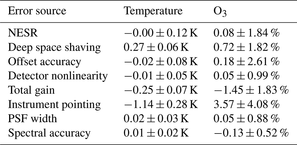
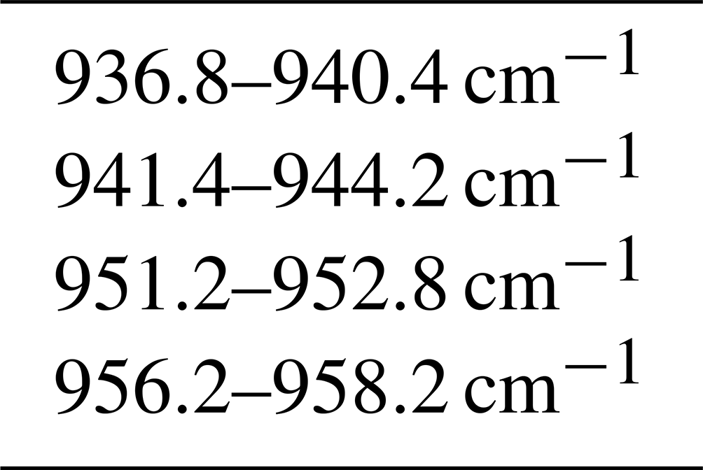
Table 6 Spectral regions used for the line-of-sight and temperature retrievals (at 0.2 cm⁻¹ resolution).

The instrument pointing has the largest impact, with a mean error of ≈1 K. The error close to flight level is smaller but increases towards lower altitudes. As LOS retrieval is typically based on ECMWF temperatures, differences from ECMWF are typically smaller than this (Johansson et al., 2018), but 1 K seems a reasonable estimate for the absolute accuracy of the temperature product. The next most important error sources are the shaving-induced offset error and the gain uncertainty. Both are of the order of 0.25 K. The other errors are an order of magnitude smaller.

The example trace gas retrieval for O₃ derives VMRs from emissions in the 1000 cm⁻¹ ozone band. The results are similar to those for the temperature retrieval. First, larger differences in temperature induce an error; second, the error source affects the ozone retrieval as well. Due to the inclusion of the strong emissions at 980 cm⁻¹, the gain error affects this retrieval especially strongly. All errors are smaller than 5 %, which is often a reasonable accuracy estimate due to given uncertainties in spectral line strength and other modeling assumptions.

These error estimates are based on the new comprehensive data basis of in-flight characterization and validation of our level 1 data quality assumptions. They are in broad agreement with prior estimates by Ungermann et al. (2015) and Johansson et al. (2018) that rely on ground-based characterization only, and hence expand on the previous studies.

7 Conclusions

The GLORIA instrument has been operated for more than 10 years. In that time, we have learned about the new challenges posed by 2-D FTIR imaging observations in general. This enabled us to make full use of all calibration data, to develop methods that statistically use atmospheric observations for in-flight validation, and to tackle a number of known instrument artifacts, several of which are specific to the 2-D concept. This mitigates some of the leading error sources in previous data versions, such as detector nonlinearity and pointing.

In this study, we have demonstrated the matured state of our calibration and level 1 processing, which forms the basis for further level 2 processing. We have exploited all three available calibration sources (the two blackbodies and the deep space measurements) to correct for the nonlinearity of our detector, which can change erratically between different cold runs of the detector. This fully solves a problem only partially addressed by previous efforts (Guggenmoser et al., 2015). The new correction allows us to use more of the available pixels, thus reducing the NESR of row-averaged spectra.

The described algorithm is able to track the noise levels of measurements during a flight in order to measure the impact of, e.g., warm blackbodies with short integration times on the calibrated data and to identify technical issues. The computed noise level of 5 nW cm⁻² sr⁻¹ cm for 0.625 cm⁻¹ is within our instrument specification.

We determine the line-of-sight calibration using both immediate measurements of celestial bodies and a level 2 product employing ECMWF temperatures. This allows us to put strong bounds on its accuracy of 0.032^∘, which corresponds to one vertical pixel.

Further, we leveraged different in-flight atmospheric measurements to get direct bounds on the accuracy of the instrument gain and offset. The gain is accurate to within 1 %, whereas the offset is subject to a potential bias of up to 30 nW cm⁻² sr⁻¹ cm.

In this fashion, we managed to put bounds on all the major error sources of our instrument, which allowed us to fully validate the existing instrument against our original instrument specification for the first time.

These aggregated errors allow us to propagate the error assumptions to level 2 products and identify the leading errors. The analysis showcases that the largest contributor of uncertainty is the line-of-sight calibration, which is already reduced to levels of the order of ±1 pixel and thus at the limit of what we can achieve with the given instrument; it also matches with the initial design specification (Friedl-Vallon et al., 2006). This uncertainty is closely followed by the uncertainty in the total gain and offset. Still, both errors are within our initial instrument target thresholds (Friedl-Vallon et al., 2014), and their impacts on level 2 data are comparable to those of other level 2 error sources such as spectroscopic uncertainties.

These advances allow us to revisit and further optimize our level 2 processing schemes. Intended improvements are, e.g., an increased vertical resolution and the VMR retrieval of additional weakly emitting trace gases, leading to new insights into the chemistry and dynamics of the UTLS region of the atmosphere. The results also demonstrate the capabilities of the imaging FTS concept in general and the opportunities of an imaging detector to increase the data quality.

Appendix A: Details on the procedure of removing atmospheric signatures from the measured deep space spectra

This section describes in detail the different steps involved in fitting the atmospheric signatures to the measured deep space spectra and the reconstruction of the forward-calculated spectra. Furthermore, it gives an estimate for the uncertainty of this method.

The spectra, which were calibrated based on the blackbody–blackbody measurements, still show a significant broadband offset that cannot be attributed to the atmosphere. It may be linked to an imperfect nonlinearity correction in combination with the large extrapolation needed to calculate the instrument offset from the two relatively warm blackbody measurements. Small errors in the blackbody temperatures may also contribute. Although the origin of this offset is not completely explained, it turns out that it is well described by a Planck function. This Planck-shaped offset is determined and subtracted in the first step. For this purpose, the offset is determined in five spectral microwindows, as listed in Table 2. In parallel, a spectral shift is fitted in each microwindow, and the resulting shifts are used to deduce a mean shift over the whole spectral range from 750 to 1400 cm⁻¹, which is then used for all further retrievals described in this section. The microwindows are selected by eye. Selection criteria are (1) the absence of broadband atmospheric emission for the offset determination, (2) one or more isolated spectral lines for the shift determination, and (3) good coverage of the spectral range. In order to obtain more stable fit results, a scale is also fitted to the data in order to compensate for imperfect VMRs in the a priori profiles.

Using the determined offset values, a Planck function is fitted to these five points, with temperature and emissivity used as fit parameters. Figure A1 shows an example median deep-space spectrum that was calibrated with the two blackbody measurements, the offset values determined in the five microwindows, and the fitted Planck function. All further plots in this section also refer to the same measurement.

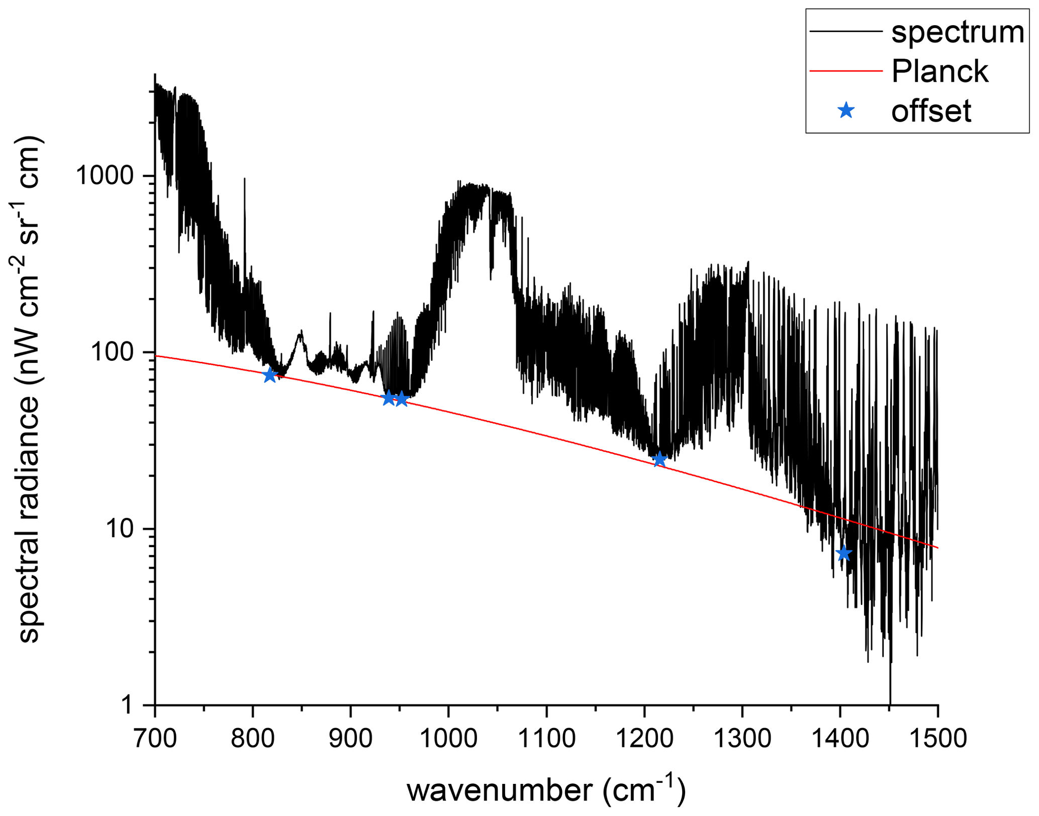
Figure A1 Median calibrated deep-space spectrum, together with the offset values at five spectral points and a Planck function fitted to the offset points. This was taken during the SouthTRAC campaign on 8 September 2019 at 07:53 Z. Please note the logarithmic scale.

In the next step, a broadband fit is performed in order to describe the measured spectrum. In total, 29 gases are considered in the forward calculation. The result of this fit is shown in Fig. A2. In general, the spectrum is well represented by the fit, and the residuals are mostly below 20 nW cm⁻² sr⁻¹ cm. There are, however, some remaining atmospheric features from, e.g., HNO₃ around 850–900 cm⁻¹, CO₂ below 800 and around 950 cm⁻¹, O₃ around 1 050 cm⁻¹, and N₂O and CH₄ at higher wavenumbers. In order to reduce the residuals, several species are fitted again in dedicated microwindows, while the fit results for all species from the broadband fit are used as new a priori profiles. For some species, it was found that dependencies on interfering species also have to be considered. For example, a simultaneous fit of CFC-11, HNO₃, and CFC-12 in the spectral window from 830 to 920 cm⁻¹ did not give satisfactory results, while fitting CFC-11 and CFC-12 in a first step and then fitting HNO₃ using the fit results for CFC-11 and CFC-12 as new a priori profiles considerably reduced the residuals. For some species (namely O₃, N₂O, and CH₄), it was not possible to represent the whole spectral range with one profile. This can be explained by inconsistencies in the spectroscopic data (e.g., Glatthor et al., 2018) or different temperature dependencies. Therefore, different profiles were fitted for different spectral ranges. The different species and microwindows for these iterations are also given in Table 2. In these iterations, an offset is also fitted for each microwindow to improve the fit result. This offset is then discarded.

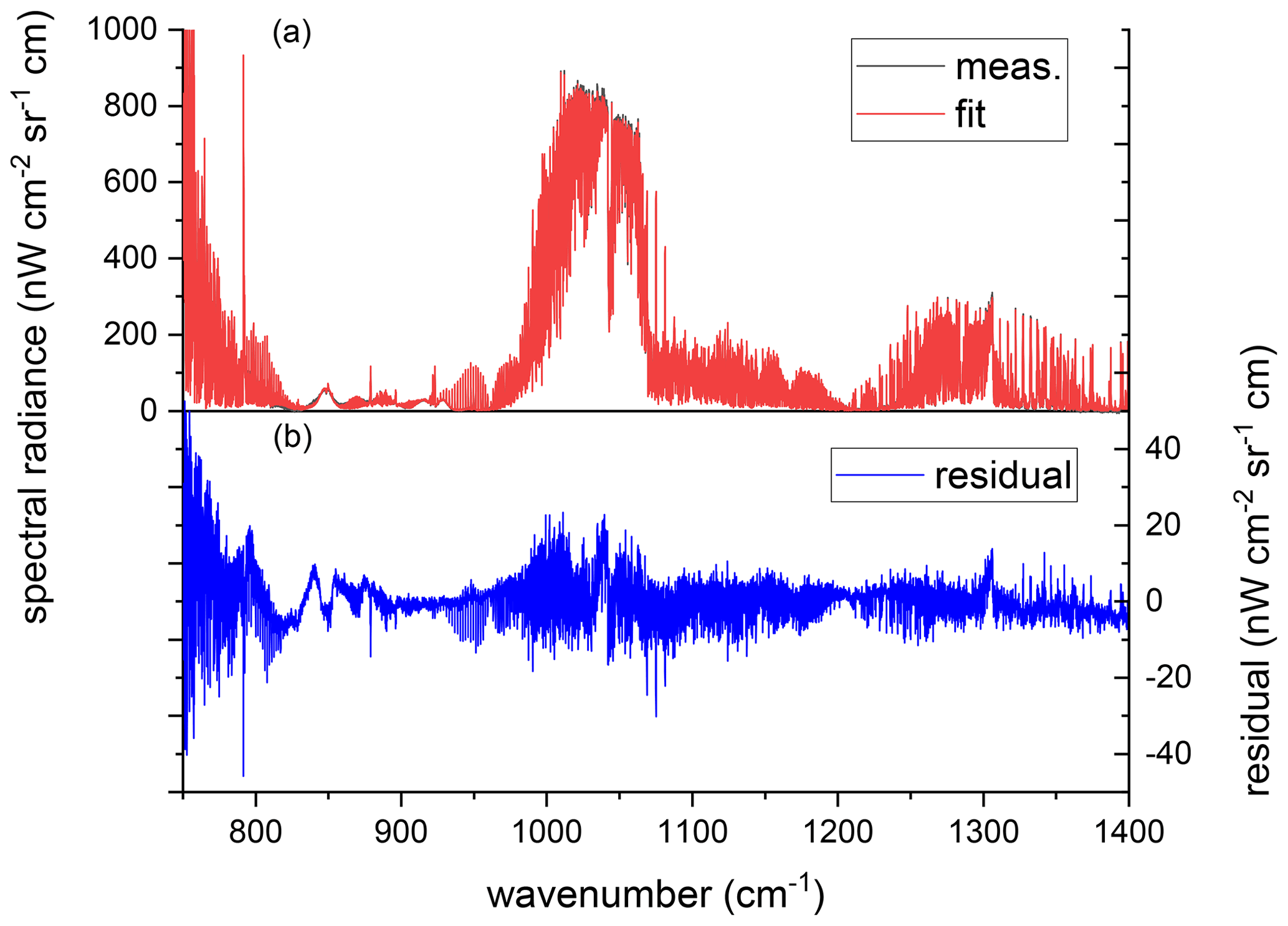
Figure A2 (a) Measurement after subtraction of the Planck function and the result of the broadband fit. (b) The residual (measurement minus fit; the right ordinate) enlarged by a factor of 10.

Figure A3 shows the improvements in the residuals after the individual fits in an example microwindow.

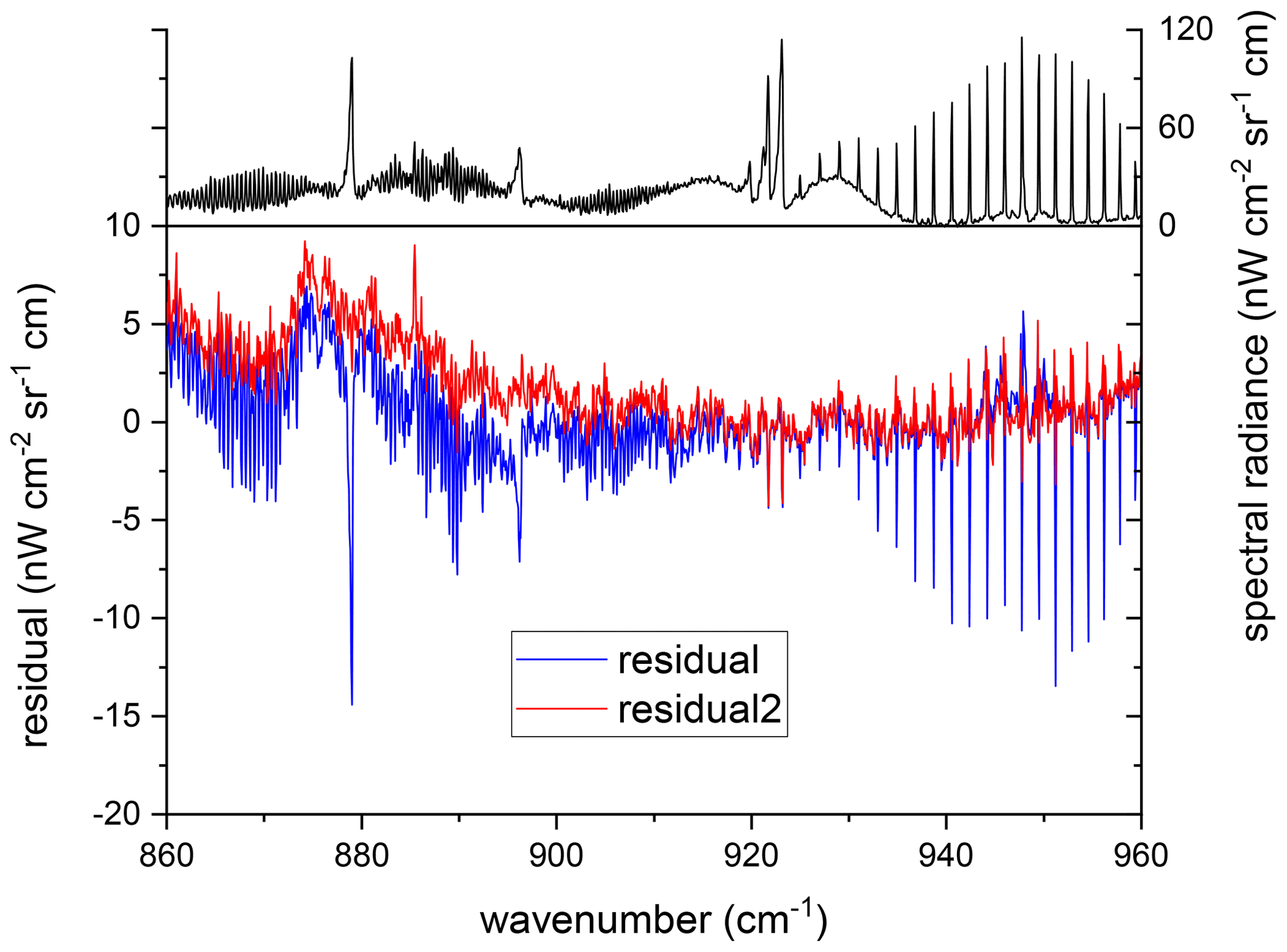
Figure A3 Residuals in the spectral range of 860–960 cm⁻¹ after the broadband fit (blue) and after fitting selected gases in individual microwindows (red). The upper panel shows the measured spectrum on the right ordinate, reduced by a factor of 12. The spectral signatures of HNO₃ and CO₂ are clearly reduced after the second fit, as is that of SF₆ around 948 cm⁻¹.

The final step in the reconstruction of the simulated spectrum is a forward calculation using the fit results of the previous steps. For O₃, N₂O, and CH₄, different profiles are used in different spectral ranges. The O₃ profile named v2 in Table 2 is used for the spectral range 850–1065 cm⁻¹; otherwise v1 is used. v0 of N₂O is used in the range 1065–1205 cm⁻¹, v1 of N₂O and CH₄ is used from 1205 to 1285 cm⁻¹, and v2 of N₂O and CH₄ is used above 1285 cm⁻¹.

The residuals between the measurement after subtraction of the Planck function and the forward calculation are considered for the estimation of the uncertainty of the instrument offset determination. These residuals are smoothed by a 10-point moving average because the offset is also calculated from smoothed spectra. In order to provide an overview of all flights and to give a representative uncertainty, the residuals of all deep space measurements of one flight are taken, and the 1σ standard deviation is calculated for each spectral point. This gives one uncertainty spectrum for each flight. These data are shown in Fig. A4. In general, the data are quite similar for all campaigns and flights, although the very early data from the TACTS campaign show rather large deviations around 830 cm⁻¹. These are attributed to the emission of the germanium entrance window, which was not fully compensated for by the calibration using the two blackbodies in this case. This was because the window correction (see Sect. 4.3) could not be applied to those data due to a malfunction of the temperature sensor. Therefore, this difference is seen as an error in calibration using the two blackbodies and is not attributed to the uncertainty of the instrument offset determination. Below 780 cm⁻¹, the deviations increase rapidly. This is attributed to a strongly increasing NESR, contributions from the window emission, and problems with the spectroscopic data. Since our nominal spectral range starts at 780 cm⁻¹, this was not considered in the uncertainty estimation.

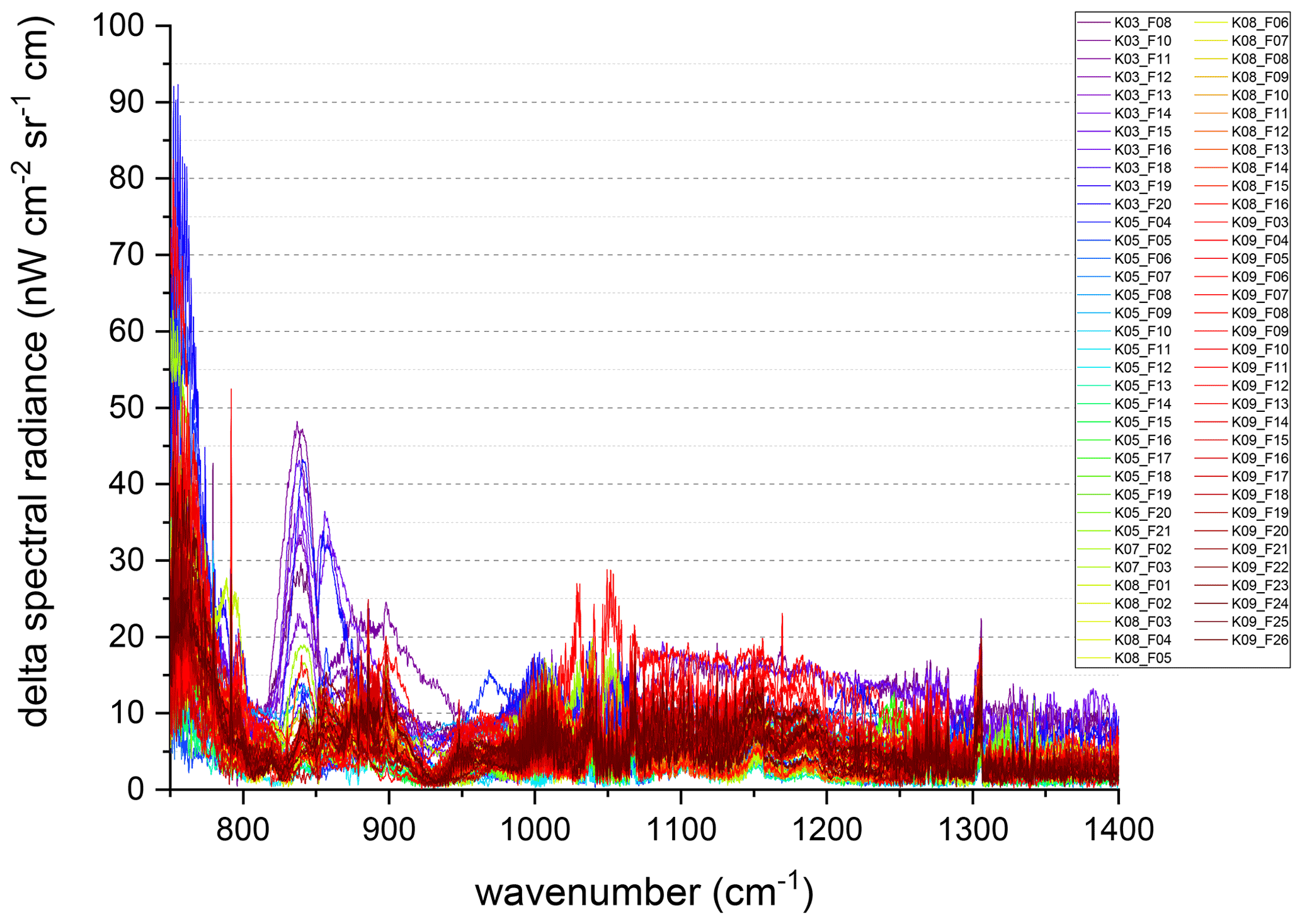
Figure A4 1σ standard deviations of the fit residuals for each flight. For details, see the text.

Other enhanced features are mainly atmospheric signatures that are not perfectly removed by our algorithm, e.g., those from CFC-11 and HNO₃ around 830–920 cm⁻¹, O₃ near 1050 cm⁻¹, and the CH₄ Q-branch at 1304 cm⁻¹. Taking these residual signatures into account, an overall 1σ uncertainty of 10 nW cm⁻² sr⁻¹ cm is derived for the whole spectral range from Fig. A4. We take the 2σ uncertainty, i.e., 20 nW cm⁻² sr⁻¹ cm, as an estimation of the systematic uncertainty due to the instrument offset determination.

Appendix B: Pixelwise nonlinearity factor determination

This section describes the computation of the pixel-specific nonlinearity correction factors in detail.

The voltage U∈ℝ measured by a detector pixel is a monotonous function $f:\mathbb{R}\mapsto \mathbb{R}$ of the incoming radiation P. Most of the nonlinearity is characterized and corrected for in an early processing step in level 0 processing (Kleinert et al., 2014), such that we have pixels that mostly show linear behavior with small variations on top. If x∈ℝ is the shift between the two arms of the interferometer position, the incoming radiation in an interferogram varies around the mean P₀∈ℝ such that one can linearize f at P₀ as follows:

$$\begin{array}{}\text{(B1)}& U\left(x\right)=f\left(P\right(x\left)\right)\approx f\left(P_{\mathrm{0}}\right)+f{}^{\prime }\left(P_{\mathrm{0}}\right)\left(P\left(x\right)-P_{\mathrm{0}}\right).\end{array}$$

For the Fourier transformation S of the interferogram U,

$$\begin{array}{}\text{(B2)}& S=\mathcal{F}\left(U\right)\approx \mathcal{F}\left(c\right)+f{}^{\prime }\left(P_{\mathrm{0}}\right)\mathcal{F}\left(P\right),\end{array}$$

where c is a constant function that only influences the zeroth frequency. Neglecting higher-order effects, this means that the uncalibrated raw spectrum is scaled with the slope of the tangent of f at the mean level P₀.

As the uncorrected nonlinearity only changes slowly with P₀, this implies that measurements with similar P₀ values and the same exposure time will be subject to effectively identical scaling factors. This applies to optically thin atmospheric and deep space measurements taken at the same exposure time. Blackbody measurements that require a much shorter exposure time and are subject to very different photon loads are problematic, as are atmospheric measurements affected by strong cloud emissions.

In the final calibration step, we deduce the instrument gain g from one deep-space and one blackbody measurement (see Sect. 3). To derive the correct gain, the different slopes induced by the different photon loads and exposure times of the blackbody measurements need to be corrected (our data analysis shows that deep space measurements are effectively similar in behavior to cloud-free atmospheric measurements) such that only one linear correction factor α needs to be determined for each detector pixel for a given blackbody measurement S_bb, as there is no spectral variation (under the assumption of no higher-order effects). With this linear scaling factor, the corrected gain g^* can be computed as

$$\begin{array}{}\text{(B3)}& g^{*}(u,v,\mathit{\nu })={\displaystyle \frac{\mathit{\alpha }(u,v)S_{\mathrm{bb}}(u,v,\mathit{\nu })-S_{\mathrm{ds}}(u,v,\mathit{\nu })}{B\left(T_{\mathrm{bb}}\right)\left(\mathit{\nu }\right)}}.\end{array}$$

Here, S_bb and S_ds refer to the raw spectra of shaved deep-space and cold blackbody measurements. u and v are the integer coordinates of the detector pixel, and ν relates to a spectral

sample.

To estimate the effect of the correction on the calibrated spectrum, one may express the corrected spectrum in terms of the uncorrected one:

$$\begin{array}{}\text{(B4)}& L={\displaystyle \frac{S}{g^{*}}}-L_{\mathrm{o}}^{*}=\left({\displaystyle \frac{S}{g}}-L_{\mathrm{o}}\right){\displaystyle \frac{S_{\mathrm{bb}}-S_{\mathrm{ds}}}{\mathit{\alpha }{S}_{\mathrm{bb}}-S_{\mathrm{ds}}}}.\end{array}$$

As the signal S_bb is much stronger than S_ds, the nonlinearity effectively causes a scaling of the calibrated spectrum. For our typical blackbody and deep-space spectra, an error of 5 % in the nonlinearity causes an error in the gain of between 4 % and 5.2 %, varying within this range both spatially and spectrally. These errors scale nearly linearly in the value range observed for our detector. The error has its largest values in the spectral regions where the entrance window of the instrument (see Sect. 4.3) has the strongest emission features and in the center of the detector, where instrument emission is smallest.

To identify the individual nonlinearity, we exploit the fact that the instrument offset L_o must be spatially smooth. As such, we define for each detector pixel (u,v) a cost function J_u,v:

$$\begin{array}{}\text{(B5)}& \begin{array}{rl}{J}_{u,v}\left(\mathit{\alpha }\right)=& \sum _{\mathit{\nu }}({\displaystyle \frac{\text{smooth}\left(\mathrm{\Re }\left(\frac{S_{\mathrm{uds}}\left(\mathit{\nu }\right)}{g\left(\mathit{\nu }\right)}\right)\right)(u,v)}{\mathrm{\Re }\left(\frac{S_{\mathrm{uds}}(u,v,\mathit{\nu })}{g(u,v,\mathit{\nu })}\right)}}\\ & -\left|{\displaystyle \frac{\mathit{\alpha }{S}_{\mathrm{bb}}(u,v,\mathit{\nu })-S_{\mathrm{ds}}(u,v,\mathit{\nu })}{S_{\mathrm{bb}}(u,v,\mathit{\nu })-S_{\mathrm{ds}}(u,v,\mathit{\nu })}}\right|{)}^{\mathrm{2}}\\ & +\mathit{\lambda }|\mathrm{1}-\mathit{\alpha }{|}_{\mathrm{2}}^{\mathrm{2}},\end{array}\end{array}$$

S_uds being the “unshaved” deep space measurement that is used to determine the correction factors for α pixel by pixel. The L_o generated by the shaved deep space is close to zero for many pixels in the center of the detector array, such that measurement noise prevents us from reliably determining the correction factors from the shaved measurements alone. The ozone band at 1000 cm⁻¹ in the unshaved deep-space spectra provides a sufficiently strong signal to reliably determine α for all pixels of the detector. The second term is a simple ad hoc regularization term to make the problem numerically well behaved. We found that λ=0.1 works well for our purposes. In addition, we exclude all ν for which the signal generated by the calibrated unshaved deep space is smaller than 200 nW cm⁻² sr⁻¹ cm. Otherwise, the noise error is amplified too much by the division in the cost function. We thus restrict the spectral range to 900–1200 cm⁻¹. Further, we average the spectral samples over 10 cm⁻¹-wide bins to reduce the number of measurements involved and thus the computational effort needed for the fit.

For function smoothing, any function capable of smoothing a 2-D grayscale image and – especially – removing shot noise would be suitable in principle (such as a median filter). We find it useful and more efficient to fit a 2-D polynomial of the 20th degree to the 2-D field, remove outliers from the fit, and refit the polynomial in a second step to generate a smooth field. Thus, we get a continuous and smooth (in the mathematical sense) 2-D function with known properties. An example of this smoothing is shown in Fig. B1: panel (a) shows the real part of the unshaved deep-space spectrum divided by the uncorrected gain for one wavenumber. This is effectively the sum of the calibrated spectrum and the instrument offset. With the continuous color scale, one can already see cluster of pixels with elevated radiance values compared to the surroundings. The noisiness becomes much more apparent in Fig. B1b, where a wrapping color scale is employed. The effect of smoothing the image with a 2-D polynomial two-step fit is shown in Fig. B1c. The polynomial tends to overshoot at the left edge of the display, where almost all the pixels are unstable due to the readout electronics. As such, the two leftmost columns are typically discarded by default in the last processing steps.

Figure B1 All: radiance offset at 964 cm⁻¹. Panel (a): the raw unshaved deep-space spectrum divided by the uncorrected gain. Panel (b): the same data, but with a color scale emphasizing irregularities. Panel (c): the image smoothed by polynomial fits. Panel (d): the raw unshaved spectrum divided by the corrected gain.

Appendix C: Description of the pointing system

The attitude is determined by an inertial measurement unit with laser gyroscopes from Honeywell (HG9900), which is mounted on the gimbal yaw frame. The attitude data are combined with information from a Novatel GPS using the Kalman filtering technique (to avoid Schuler oscillations for example). To ensure high stability of the pointing, a three-axis microelectromechanical (MEMS) gyroscope from Sensonor is mounted on the pitch (elevation) frame. The orientation of the gimbal frame is measured by inductive angular encoders (WMK series) from AMO GmbH, which are robust under the harsh conditions of an open compartment, even under slight icing conditions. All these data are fused by a stabilization control unit to provide both fast attitude changes and stabilization of the FOV. The needed agility is realized by direct-drive motors from Robodrive and independent drive controller units from Elmo Motion Control. This inertial measurement and stabilization control unit (iIMCU) was developed by iMAR Navigation GmbH, Germany.

This pointing system allows several control modes that are connected to the observation scenarios needed for GLORIA. For atmospheric measurements with high spatial resolution, the control system switches to target mode, which works like a point-and-stare mode. During the acquisition of one interferogram, the LOS of one defined pixel is stabilized to a specific point defined in WGS84 coordinates. Then, step by step, the azimuth is turned by a certain angle, and the next point is stabilized. The coordinates are calculated using predefined patterns with a gimbal yaw angle step size of typically 4–8^∘ and a dwell time of several seconds, depending on the configured spectral resolution of the interferometer.

For atmospheric measurements with high spectral resolution, the altitude-azimuth mode is used. FOV stabilization is focused on a given tangent altitude and azimuth in the WGS84 system for a specified pixel. Contrary to the target mode, the horizontal movement of the aircraft is not compensated for, but the azimuth is kept constant during the acquisition of one interferogram, leading to slight horizontal smearing of the tangent point. In both modes, the elevation is continuously adjusted to keep the altitude of the tangent height of a specified pixel constant, even during variations in the flight altitude.

The nadir mode also acts as a point-and-stare mode, like the target mode, but is designed to stabilize a foot print on the ground through an aperture in the bottom of the belly pod.

Deep-space calibration measurements are performed with an elevation of 10^∘ in the angle mode of the pointing system and with the stabilization of constant elevation and azimuth angles defined in WGS84.

Blackbody calibration measurements are performed in gimbal mode with fixed positions of the gimbal mount in order to point to one of the two internal blackbodies.

All pointing changes are synchronized to the short breaks in interferogram acquisition when the slide in the interferometer changes direction in order to avoid scene jumps in the interferogram data.

Appendix D: Determining the position of the moon

To determine the position of the moon in relation to the instrument with high accuracy, we make use of the JPL ephemeris data in version DE421. We use the Python software package Skyfield to access the JPL data and determine the apparent altitude and azimuth at the instrument's position, including relativistic effects and aberration (Rhodes, 2019). Even though the moon measurements were taken at 12 km altitude and above, the refraction of the atmosphere cannot be neglected, especially as some moon measurements were taken below the horizon. The Skyfield package computes refraction, but only for up to −1^∘, which is a reasonable value at ground level but insufficient for our purposes. Lacking a readily available formula for computing the refraction under the given conditions, we determine the effect of refraction by the straightforward ray-tracing algorithm given below.

Earth is assumed to be spherical, and the ray is traced in a plane with polar coordinates (r,θ) and the origin at the center of the Earth. The coefficient of refraction n(r) is computed using atmospheric profiles for temperature and pressure taken from ECMWF analysis data at the instrument's position. Let the ray be described by r=r_r(θ), and let the angle between the ray and vertical be ϕ(r_r(θ),θ). We backtrace the ray from the instrument at position (r₀,0) with ϕ=ϕ₀. In the absence of refraction, the ray would be a straight line with $\mathit{\varphi }={\mathit{\varphi }}_{\mathrm{0}}-\mathit{\theta }$, so, for the refracted ray, we can write $\mathit{\varphi }={\mathit{\varphi }}_{\mathrm{0}}-\mathit{\theta }+\mathit{\delta }\left({\mathit{\varphi }}_{\mathrm{0}},r_{\mathrm{0}},n\left(r\right)\right)$, where the angle δ represents the deviation from the straight line.

$$\begin{array}{}\text{(D1)}& {\displaystyle \frac{\mathrm{d}\mathit{\delta }}{\mathrm{d}\mathit{\theta }}}={\displaystyle \frac{\partial \mathit{\delta }}{\partial n}}{\displaystyle \frac{\partial n}{\partial r}}{\displaystyle \frac{\mathrm{d}{r}_{\mathrm{r}}}{\mathrm{d}\mathit{\theta }}}.\end{array}$$

Snell's law gives $\mathrm{d}\left(n/\sin \mathit{\varphi }\right)=\mathrm{0}$ for any point on the ray path, so $\mathrm{d}\mathit{\delta }/\mathrm{d}n=\mathrm{d}\mathit{\varphi }/\mathrm{d}n=\tan \mathit{\varphi }/n$. From basic geometry in polar coordinates, $\partial r_{\mathrm{r}}/\partial \mathit{\theta }=r_{\mathrm{r}}/\tan \mathit{\varphi }$. Using these two relations and Eq. (D1), we formulate the backtracing of the ray as an initial value problem:

$$\begin{array}{}\text{(D2)}& \left\{\begin{array}{lcl}\frac{\partial \mathit{\delta }}{\partial \mathit{\theta }}& =& \frac{r}{\widehat{n}+\mathrm{1}}\frac{\partial \widehat{n}}{\partial r}\\ {\displaystyle \frac{\partial r}{\partial \mathit{\theta }}}& =& \frac{r}{\tan \left({\mathit{\varphi }}_{\mathrm{0}}-\mathit{\theta }+\mathit{\delta }\right)}\\ \mathit{\delta }\left(\mathrm{0}\right)& =& \mathrm{0}\\ r\left(\mathrm{0}\right)& =& r_{\mathrm{0}},\end{array}\right.\end{array}$$

where the variable $\widehat{n}=n-\mathrm{1}$ has been introduced for numerical stability, as $n-\mathrm{1}\ll \mathrm{1}$. We solve this numerically to obtain $\mathit{\varphi }{|}_{r\to \mathrm{\infty }}\approx \left({\mathit{\varphi }}_{\mathrm{0}}-\mathit{\theta }+\mathit{\delta }\right){|}_{r=\mathrm{2}{R}_{\mathrm{0}}}$, with R₀ being the mean Earth radius. We then iterate the interval, halving to get the moon's elevation $\mathit{\pi }/\mathrm{2}-{\mathit{\varphi }}_{\mathrm{0}}$ as a function of the (known) astronomical elevation $\mathit{\pi }/\mathrm{2}-\mathit{\varphi }{|}_{r\to \mathrm{\infty }}$, r₀ and n(r).

In a final step, we identify the position of the moon in the infrared images by manually matching a circle of the expected moon size with the taken images (see Fig. 14). We expect an uncertainty from this process of about 1 detector pixel for visual identification and 0.02^∘ for refraction and positioning, corresponding to a total of 0.05^∘ for both azimuth and elevation.

Appendix E: Standard atmosphere profiles

Several of our methods require standard atmospheric profiles for a range of trace gases. We typically use the profiles collected by Remedios et al. (2007) for this purpose. Comparing forward calculations made using these profiles to our recent measurements revealed noticeable discrepancies of the order of several nW cm⁻² sr⁻¹ cm associated with CCl₄, CH₄, CO₂, CFC-11, CFC-12, CFC-14, CFC-113, HCFC-22, SF₆, and N₂O. While these discrepancies can be partly associated with the fact that a climatological standard profile will almost never fully agree with the actually obtained one, we found that, especially for the upwards-pointing stratospheric deep-space measurements, a large part of the discrepancy was caused by changes in atmospheric composition between the creation of the dataset and the time of measurement.

To improve the climatological profiles, especially for the shaving procedure, we retrieved global monthly data for these species from the Halocarbons & other Atmospheric Trace Species (HATS) research program (e.g., Hu et al., 2016; Montzka et al., 2021, 1996; Elkins and Dutton, 2009; Montzka et al., 2009; Conway et al., 1994; Dlugokencky et al., 1994). We further smoothed the data by computing a running mean over 12 consecutive months and fully disregarded differences between the hemispheres for simplicity. For HCFC-22 and CFC-14, no such globally averaged product was available at the time; instead, measurement data from several individual stations were given. We computed a crude global average over the available stations and performed a running yearly mean to derive a similar product to that given for the other species.

To update the profiles of Remedios et al. (2007), we simply scaled the full profile (and the associated standard deviation) with a multiplicative factor derived from the quotient between the value of the HATS data and the ground-level value of the profile. This improved the fit to the radiances and reduced visible residuals caused by these interfering species, thus reducing the systematic error induced by emissions from these trace gases.

Appendix F: Level 2 processing

F1 Line-of-sight/temperature retrieval

To determining the line of sight from measured data with a spectral resolution of 0.2 cm⁻¹, we assume that temperature values supplied by ECMWF analysis data are close to real values. In effect, we perform a standard retrieval, keeping the temperature at ECMWF values and only varying the elevation correction value until the best fit of the simulated measurements to the measured ones is achieved. A very rough error estimate for this approach shows that, with gradients of ≈10 K km⁻¹, a systematic 1 K error in ECMWF would cause an error in the final pointing data of only about 100 m. The situation becomes even better when the profiles contain both tropospheric and stratospheric sections with temperature gradients of opposite signs. Still, wrongly represented tropopauses, gravity waves, or other nonuniform biases in temperature impact the method. Thus, we (generally) do not place our trust in individual values but in the average over a whole measurement flight after filtering short profiles with high uncertainties.

The retrieval itself leverages CO₂ emission lines around 950 cm⁻¹, where only a few other gases have interfering emissions. Table 6 shows the spectral regions used. These were selected to avoid strong emission features by, e.g., CFC-12, O₃, H₂O, and SF₆, and to cover as many CO₂ lines as feasible. The retrieval uses the trace gases CO₂, CFC-12, and SF₆ with climatological values (see Appendix E). For H₂O, we use water vapor, as given in the ECMWF analysis data, even though the impact of this is small. In addition to the line of sight, an extinction profile is also retrieved to capture both atmospheric aerosol and small calibration errors.

To derive the temperature instead, we simply revert the roles of line of sight and temperature. We use smoothed ECMWF temperatures as the a priori and initial guess (but the choice of a priori typically does not affect the results, only the convergence speed). In addition to temperature, this setup also derives PAN as a secondary target in order to remove its (small) influence in polluted air.

F2 O₃ retrieval

The ozone retrieval discussed briefly in Sect. 6 is a simplified version of the retrieval described by Ungermann et al. (2015). It uses the four spectral regions listed in Table F1, each averaged to a single radiance. The temperature and PAN values derived from the temperature retrieval of Sect. F1 are used, as well as the ECMWF analysis of water vapor. The retrieval derives only O₃ VMRs and a single extinction profile. Climatological values are employed for the trace gases CO₂, CFC-12, CFC-113, NH₃, and SF₆ (see Appendix E).

Table F1 Spectral regions used for the O₃ retrieval (0.2 cm⁻¹ resolution).