the Creative Commons Attribution 4.0 License.
the Creative Commons Attribution 4.0 License.
 | 29 Apr 2022
Development and application of a supervised pattern recognition algorithm for identification of fuel-specific emissions profiles
Christos Stamatis
Kelley Claire Barsanti
Wildfires have increased in frequency and intensity in the western United States (US) over the past decades, with negative consequences for air quality. Wildfires emit large quantities of particles and gases that serve as air pollutants and their precursors, and can lead to severe air quality conditions over large spatial and long temporal scales. Therefore, characterization of the chemical constituents in smoke as a function of combustion conditions, fuel type and fuel component is an important step towards improving the prediction of air quality effects from fires and evaluating mitigation strategies. Building on the comprehensive characterization of gaseous non-methane organic compounds (NMOCs) identified in laboratory and field studies, a supervised pattern recognition algorithm was developed that successfully identified unique chemical speciation profiles among similar fuel types common in western coniferous forests. The algorithm was developed using laboratory data from single fuel species and tested on simplified synthetic fuel mixtures. The fuel types in the synthetic mixtures were differentiated, but as the relative mixing proportions became more similar, the differentiation became poorer. Using the results from the pattern recognition algorithm, a classification model based on linear discriminant analysis was trained to differentiate smoke samples based on the contribution(s) of dominant fuel type(s). The classification model was applied to field data and, despite the complexity of the contributing fuels and the presence of fuels “unknown” to the classifier, the dominant sources/fuel types were identified. The pattern recognition and classification algorithms are a promising approach for identifying the types of fuels contributing to smoke samples and facilitating the selection of appropriate chemical speciation profiles for predictive air quality modeling using a highly reduced suite of measured NMOCs. The utility and performance of the pattern recognition and classification algorithms can be improved by expanding the training and test sets to include data from a broader range of single and mixed fuel types.
- Article
(1916 KB) - Full-text XML
-
Supplement
(1269 KB) - BibTeX
- EndNote


Research has showed that the western United States (US) has seen an increase in the frequency and intensity of wildfires over the last three decades (Jaffe et al., 2020; Miller et al., 2009; Dennison et al., 2014), which is projected to continue (Westerling et al., 2006; Miller et al., 2009; Dennison et al., 2014). One of the consequences of wildfires is extremely poor air quality (McMeeking et al., 2005; McKenzie et al., 2006; Park et al., 2006; Hu et al., 2018). Emissions from wildfires include carbon monoxide (CO), carbon dioxide (CO2), and methane (CH4); several hundreds of gas-phase non-methane organic compounds (NMOCs); and particulate matter (PM). While CO2 and CH4 are important greenhouse gases, NMOCs are of particular importance in the context of air quality because they serve as precursors to secondary air pollutants, including photochemical ozone (O3) and secondary organic aerosol (SOA) (Andreae et al., 1988; Ward and Hardy, 1991; Alvarado and Prinn, 2009). The latter (SOA) is a major constituent of atmospheric PM (Zhang et al., 2007). In order to predict the air quality impacts of wildfires, differences in emissions and their effects on chemistry and pollutant formation must be represented in models (Kochanski et al., 2015; Pavlovic et al., 2016; Chen et al., 2019; Prichard et al., 2019; Jaffe et al., 2020). Wildfire emissions are dependent on a number of factors, such as combustion conditions (e.g., flaming vs. smoldering), fuel conditions (e.g., moisture content) and fuel type (e.g., species and component) (Goode et al., 2000; Urbanski, 2013; Liu et al., 2017; Stockwell et al., 2014, 2015; Koss et al., 2018; Sekimoto et al., 2018; Hatch et al., 2019; Prichard et al., 2020). Differences in these factors can affect the total amount of emissions as well as the profile of emissions, i.e., the identities and quantities of individual chemical species. Permar et al. (2021) recently reported that combustion conditions, specifically modified combustion efficiency (MCE), explained approximately 70 % of the variability in observed trace gas emissions from wildfires. Consistent with some existing modeling approaches, they suggested that total NMOCs could be predicted using MCE and that the contributions of individual compounds could be determined using speciation profiles. For this approach to be successful, knowledge of the relevant speciation profiles, and therefore the contributing fuel types, is required.
NMOC speciation profiles have been developed from both field and laboratory studies (Urbanski et al., 2008; Urbanski, 2014; Simpson et al., 2011; Holder et al., 2017; Andreae, 2019; Prichard et al., 2020). Laboratory studies offer some advantages over field studies in the context of controlling fuel species and fuel components; other variables, such as combustion conditions and fuel moisture, can be harder to control and can lead to differences in the identities and quantities of NMOCs emitted between laboratory and field studies (Yokelson et al., 2013; Stockwell et al., 2014; Liu et al., 2017; Sekimoto et al., 2018). Yokelson et al. (2013) presented an intercomparison of laboratory- and field-based emission factors (EFs) as well as approaches that combine the use of laboratory data to enhance the fundamental understanding of fire emissions with the use of field data to evaluate the representativeness of laboratory-based measurements. At that time, they noted that up to 70 % of NMOCs remained unidentified for certain fuel types. More recently, due to the application of advanced instrumental techniques, there have been significant improvements in the identification and quantification of NMOCs emitted from fires, particularly in laboratory studies (Stockwell et al., 2014, 2015; Hatch et al., 2017; Koss et al., 2018). For example, Stockwell et al. (2015) detected approximately 80–96 % of the total emitted NMOC mass in experiments during the fourth Fire Lab at Missoula Experiment (FLAME-4) in 2012, and Hatch et al. (2019) identified more than 500 individual NMOCs during FLAME-4. The relatively rapid expansion in available NMOC data provides opportunities for developing more detailed speciation profiles (in which a higher fraction of the detected mass is assigned to unique compounds or formulas) and for applying statistical data analysis methods, facilitating the identification of unique sets of compounds that allow the differentiation of fuel type(s) and the estimation of their contributions to smoke samples.
Existing approaches for identifying the contribution of fuel types to smoke include land cover databases or fuel loading models coupled with fuel consumption models (e.g., FOFEM, Keane and Lutes, 2018; and CONSUME, Ottmar, 2009), and the use of marker compounds. One of the limitations of land cover databases or fuel loading models is that they are difficult to update frequently enough to reflect changes in ecosystems (Reeves et al., 2009; Vogelmann et al., 2011; Nelson et al., 2013; Lindaas et al., 2021). Marker compounds are emitted in relatively high abundances and can be used to differentiate fuels by component or fuel layer and, in some cases, by species. For example, Wan et al. (2019) showed that p-hydroxybenzoic acid was emitted from the combustion of herbaceous plants, while vanillic acid was emitted from the combustion of softwoods and hardwoods. It has also been shown that syringic acid is associated with hardwood combustion (Simoneit, 2002; Zangrando et al., 2013), and dehydroabietic acid with conifers (Fu et al., 2009). Zhang et al. (2021) found that the benzene-to-toluene ratio in smoke from sugarcane leaves was different than the ratio in smoke from sesame stalk, demonstrating differences among agricultural fuels. In measurements of western forests and shrublands, Jen et al. (2018) showed that hydroquinone was a good marker for manzanita combustion. One of the limitations of using marker compounds to identify fuel types is the lack of specificity, i.e., marker compounds have not been identified that enable the identification of a large number of fuel species or closely related fuel species.
In this work, a method is presented for identifying fuel types from measured NMOCs in smoke samples. To overcome some of the existing limitations in identifying the contributions of specific fuel types to smoke, pattern recognition (PR) and classification algorithms were developed using data obtained during two laboratory campaigns in 2012 and 2016, and these algorithms were applied to data obtained during a field study in 2017. Machine learning techniques have been applied for source identification in other disciplines. For example, Welke et al. (2013) and Ziółkowska et al. (2016) used principal component analysis (PCA) and linear discriminant analysis (LDA) to differentiate and classify wine varietals based on specific compounds present in wine samples. Johnson and Synovec (2002) used PCA and analysis of variance to select marker compounds in gasoline fuel blends and PR to differentiate the blends. In this work, the large data sets generated during FLAME-4 and the Fire Influence on Regional to Global Environments Experiment (FIREX) Fire Lab 2016 campaigns were leveraged to develop a source identification method using fuel-specific NMOC profiles. The PR algorithm performs an automated selection of compounds that differentiate sources (in this case fuels) based on measured NMOCs. The classification algorithm then uses the source profiles to identify source contributions to specific samples. The data used to train and test the algorithm are introduced in Sect. 2. The algorithm development, implementation and testing are presented in Sects. 2 and 3. The application to field data is presented in Sect. 3, and general conclusions and implications are presented in Sect. 4.
2.1 Data
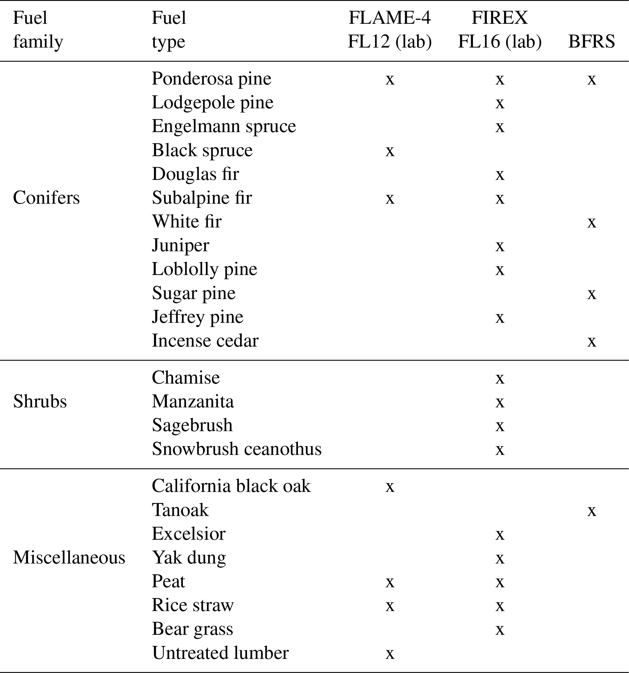
The NMOC data used in this study were acquired from a variety of fuel types burned in laboratory and field settings during three campaigns: (1) the FLAME-4 laboratory campaign in 2012 (FLAME-4 FL12), (2) the FIREX laboratory campaign in 2016 (FIREX FL16), and (3) Blodgett Forest Research Station (BFRS) prescribed burns in 2017. Both laboratory campaigns took place at the US Forest Service Fire Science Laboratory (FSL). Details of the facilities, sample collection and data analysis have been discussed in previous publications (Stockwell et al., 2014; Hatch et al., 2015, 2019; Selimovic et al., 2018). Briefly, during FLAME-4 FL12 and FIREX FL16, a broad variety of biomass fuels were burned (Stockwell et al., 2014; Selimovic et al., 2018), including conifers and shrubs (Table 1); 80 samples were collected from both room and stack burns, as described in Stockwell et al. (2014) and Selimovic et al. (2018). During the BFRS study, a total of 28 samples (Hatch et al., 2019) were collected from a utility task vehicle parked downwind from three separate prescribed burn plots that had different fuel distributions (see Table 1 and Supplement Figs. S2–S4 in Hatch et al., 2019). All NMOC samples were collected using dual-bed stainless steel sorbent tubes and were analyzed using an automated thermal desorption unit coupled to a two-dimensional gas chromatograph with a time-of-flight mass spectrometer (GC × GC-TOFMS). The raw chromatograms were processed using the commercially available software Chromatof (Leco Corp., St. Joseph, MI, USA). The measured mixing ratios were used to calculate normalized excess mixing ratios (NEMRs) versus CO, CO (Yokelson et al., 1999), in which Δ represents excess over background. The calculated NEMRs of monoterpenoids (C10H16 and C10H16O) were used as the starting point for this analysis based on Hatch et al. (2018, 2019), and the emission profile analysis is presented in Sect. S1 in the Supplement. Hatch et al. (2019) demonstrated that the variability in NMOC composition could not be attributed entirely to the MCE, and that chemical speciation was highly correlated among some fuel types across a range of MCE values, particularly for conifers, where clear differences in monoterpenoid emissions were observed as a function of fuel species.
Table 1Fuels burned and smoke analyzed from FLAME-4 2012 laboratory fires, FIREX 2016 laboratory fires and Blodgett Forest Research Station prescribed burns.
2.2 Pattern recognition algorithm
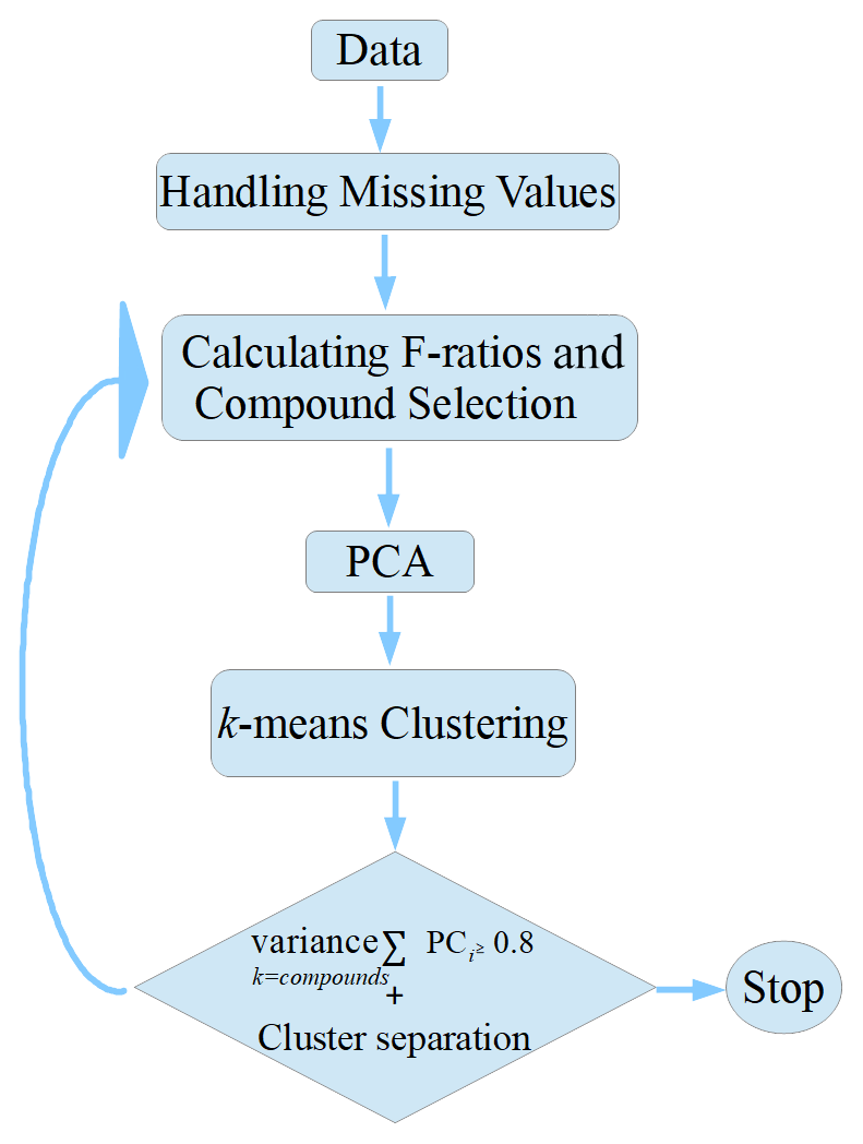
A four-step PR algorithm (Fig. 1) was developed to select a subset of compounds that captured the variance between fuel types and then use the selected compounds to differentiate fuel types based on NMOC speciation profiles. The algorithm steps are (1) data preprocessing, (2) analysis of variance (ANOVA), (3) principal component analysis (PCA) and (4) k-means clustering. The algorithm was implemented using the Python package scikit-learn (Pedregosa et al., 2011). The algorithm components are explained in Sect. 2.2.1–2.2.4. Implementation of the algorithm is explained in Sect. 2.3.
2.2.1 Preprocessing and analysis of variance (ANOVA)
Data preprocessing (step 1) is performed to handle any missing values in the samples. Approaches for handling missing values are specific to the type(s) of data and the reason(s) for missing values (Dong and Peng, 2013; McNeish, 2017). In this data set, missing values largely were a result of compounds being below the detection limit or having negative values after background correction. During preprocessing, for every feature (i.e., compound), the percentage by number of missing values across all samples was calculated. For any given compound, if the percentage of missing values was less than 30 %, then the missing values were replaced with zeros. If the percentage was more than 30 %, then the compound was removed from the data set. The 30 % threshold is supported by published statistical method guides, including Dong and Peng (2013) and Jakobsen et al. (2017), which suggest a threshold range of 10–40 % prior to replacement.
Samples were also evaluated and filtered for missingness, using two criteria. For criterion one, only fuel types that had more than 30 % (by number) of the 93 monoterpenoids above background levels were selected. Since the PR algorithm was based on monoterpenoids, samples with few to no detected monoterpenoids would reduce the ability of the algorithm to differentiate between fuel types and therefore reduce the overall efficiency. For criterion two, only fuel types that had three or more samples were retained. For fuels with too few samples, the necessary statistical properties cannot be calculated. In addition, the second criterion ensured that the remaining fuel types had an approximately equal number of samples in the analysis.
Feature selection (step 2) reduces the number of variables by selecting only those that are informative. In this work, an analysis of variance (ANOVA)-based feature selection method similar to those used in Johnson and Synovec (2002) and Welke et al. (2013) was used to further filter the compounds retained in step 1. In this application, each detected compound was treated as an ANOVA-type problem with N samples in k classes (fuel types) to determine whether or not a compound could separate the different fuel types. For each compound, the ratio of class-to-class variance to within-class variance, also known as the Fisher ratio (F-ratio), was calculated using
where the nominator (Vb) corresponds to the between-class sum of squares and the denominator (Vw) to the within-class sum of squares. The magnitude of the F-ratio is an indication of class separation. Following the F-ratio calculation, the compounds were ranked in ascending order based on their F-ratios. Further details regarding the F-ratio calculation can be found in Sect. S2 in the Supplement.
2.2.2 Principal component analysis (PCA)
Principal component analysis (PCA; step 3), as described in Abdi and Williams (2010), is a dimensionality reduction technique that is used to project high-dimensional data into a lower-dimensional space along the direction(s) of maximum variance in the data. In PCA, the original variables are transformed into a new coordinate system. The new coordinate system is formed using the calculated principal components (PCs), which serve as the new directions/axes. Each PC is a linear combination of the original variables and weights (also called loadings), as shown in
where i and j are indices corresponding to the number of PCs and number of original variables, respectively. Each PC accounts for a specific amount of variance of the observed data, with the first accounting for the greatest amount and each succeeding component an amount less than the previous. The PCs can be calculated either by eigenvalue decomposition (EVD) on the covariance matrix of the original data or by singular value decomposition (SVD) on the data matrix. In this study, SVD was used; the implementation of SVD is further described in Sect. S3 in the Supplement. Regardless of the method being used to calculate the PCs, because PCA is trying to find new axes along the direction(s) of maximum variance, if the variables are not on the same scale or if there is a large difference in the magnitudes, the results can be biased in favor of the variable(s) that vary on a larger scale (Gewers et al., 2021; Lever et al., 2017). For this reason, standardization of the data might be necessary prior to PCA. In standardization, the data are mean centered and each variable is divided by the standard deviation of that variable. While standardization can help alleviate the scaling problem, it should not be a default practice, as it can magnify the effect of outliers in the data (Gewers et al., 2021). If the variability of a feature is a consequence of intrinsic variability in the analytical method (e.g., experimental error or noise in the data), then standardization may erroneously emphasize that in the PCA results. In such cases, either the noise should be reduced by some means or standardization should be avoided. In this study, the selection of PCA for dimensionality reduction was based on three previous studies that included PCA in pattern recognition analysis of chromatographic data (Welke et al., 2013; Johnson and Synovec, 2002; Ziółkowska et al., 2016).
2.2.3 k-means clustering
k-means (step 4) is a popular clustering algorithm that finds clusters in an n-dimensional space (Jolliffe, 2002). Given a set of observations (x1, x2, x3, ..., xn), where each observation is a d-dimensional real vector, k-means tries to partition the n observations into k ≤ n sets S = {S1, S2, S3, ..., Sk}. Mathematically, k-means clustering minimizes within-cluster variances, or squared Euclidean distances (Jain, 2010), as shown in
where μi is the mean of the points in Si. In this study, Elkan's algorithm (Elkan, 2003) was used to solve Eq. (3). k-means clustering was used to find clusters formed after the application of PCA. The inputs for the clustering analysis were the retained PCs. k-means was chosen over other clustering algorithms because of its simplicity and the absence of highly anisotropically distributed clusters (irregular shapes); unequal variance among the clusters and unevenly sized clusters can cause problems with k-means (Jain, 2010).
2.2.4 Determining the number of principal components and clusters
Three metrics for determining the number of components retained after PCA were considered: (1) explained variance based on the number of retained components, (2) the Kaiser criterion, and (3) the scree test. The explained variance % (Eq. S8 in the Supplement) evaluates how much of the original variance in the data is explained by each additional component retained. For this metric, there is no strict threshold; 80 % was chosen for this study. The Kaiser criterion suggests rejecting all factors that have eigenvalues less than 1. The scree test requires plotting the eigenvalues as a function of component number; an inflection point indicates the maximum number of usable components. The default method used in this study was the explained variance, but all three approaches were evaluated and provided similar results.
k-means requires that the target number of clusters is provided in advance. This is challenging when the number of clusters is not known. In this study, the elbow plot method was used to determine the number of clusters (Fig. 5). The elbow plot method requires running the k-means multiple times using a different number of clusters each time. For each run, the total within-sum of squares (TWSS) was calculated according to
where q and c are multidimensional vectors with the coordinates for each centroid and sample, respectively; n is the total number of samples and kmax is the total number of preselected clusters. TWSS is a measure of variability for the observations within a cluster. The smaller the TWSS for a number of clusters, the better the clustering. TWSS is plotted against the number of clusters. As with the scree test, the inflection point in the plot signifies the optimum number of clusters.
2.3 Running the pattern recognition algorithm
Implementation of the PR algorithm proceeds through five steps. In step 1, the compounds in the data set are preprocessed to replace missing values and discard samples that might be problematic (Sect. 2.2.1). In step 2, for each retained compound, the F-ratio is calculated. In step 3, in an iterative fashion, PCA and k-means clustering are performed on the m highest-ranked compounds, and the separation of the classes in the samples (fuel types) is evaluated as a function of the number of compounds and the minimum number of PCs that achieve the 80 % variance threshold. In step 4, if the separation is not adequate, then the number of compounds is increased or decreased and the run is repeated. In step 5, once the class separation no longer improves or starts degrading with the addition or removal of compounds (step 4), more PCs are retained and different combinations of PCs are tested. While increasing the number of components will lead to better separation of the fuel types, it can also lead to overfitting. In this study, the algorithm was optimized for sample separation as a function of the compounds selected and the pairing of the PCs. The effects of overfitting were not considered in the optimization due to limitations on the sample size that prevented the use of known evaluation methods.
2.4 Classification
To test the applicability of the PR algorithm results for field samples, a classification algorithm, LDA (Hastie et al., 2009), was applied (see Sect. S5 in the Supplement for implementation details). LDA is a supervised learning method that is similar to PCA. Both LDA and PCA are linear transformation techniques; LDA is supervised, whereas PCA is unsupervised and ignores class labels. While PCA tries to find a subspace of features in order to maximize variance among samples, LDA attempts to find a feature subspace that maximizes class separability. The inputs for the LDA training were the selected PCs from the PR analysis (independent variables) and the fuel types (response variable/class) (see Sect. S4 in the Supplement). The output of LDA is a probability score for every sample that is being tested for its likelihood to belong to a particular fuel type, calculated as follows:
where k is the class of sample x, μ is the vector of the means for each class based on the selected features, Σ is the common covariance matrix for the three classes in the training set and Cst is a term that contains a constant from the multivariate Gaussian distribution. LDA was chosen as the classification method in this study because its closed-form solution does not require any hyperparameter tuning. Methods that require hyperparameter tuning (e.g., k-nearest neighbors) are not appropriate for this application because (1) the training data set included laboratory data only while the test set included field data and (2) the field data were not labeled.
3.1 Sample and fuel type selection for pattern recognition and classification
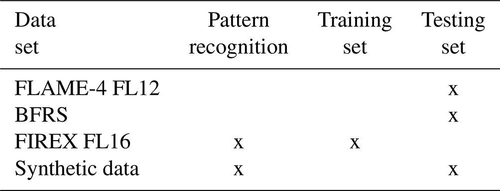
The PR algorithm was applied to the FIREX FL16 data set to identify a group of marker compounds that could be used to differentiate fuel types. Classification was then performed using the FIREX FL16 data as the training set and BFRS data as the testing set. The selection of the training and testing sets was based on the size of each data set; the FIREX FL16 data set had 74 samples and the BFRS data set had 29 samples. A larger training set ensured more statistically robust parameters for the LDA model. Because BFRS samples were generated from combustion of complex fuels, a synthetic data set was generated to test the performance of the PR and classification algorithms on mixed fuel samples prior to application on the BFRS data. The synthetic samples were created by taking the average value of each selected NMOC from each fuel type and linearly combining them using specific percentages for two fuels (e.g., 60/40 and 90/10). The five synthetic mixtures had the following compositions: 60 % pine/40 % spruce, 60 % fir/40 % spruce, 60 % pine/40 % fir, 90 % pine/10 % spruce and 90 % fir/10 % spruce. The FLAME-4 FL12 data were used as an independent data set to test the response of the classification algorithm to fuel types that were not included in the training set. The use of each data set in the PR and classification algorithms is summarized in Table 2.
Before applying the PR algorithm, the data were processed as described in Sect. 2.2.1. Application of the preprocessing criteria reduced the number of samples from a total of 74 to 39 and the number of fuel species from 18 to five: pines (ponderosa pine and lodgepole pine), firs (Douglas fir and subalpine fir) and spruce (Engelmann spruce). During the FIREX FL16 study, different fuel components were burned, such as canopy, rotten log, composite, litter and duff. While differences in component emissions may be important for differentiating prescribed burn and wildfire smoke samples, for this application, 32 composite and canopy samples and seven litter and duff samples were retained based on the selection criteria (Sect. 2.2.1).
Table 2Data sets used for developing the pattern recognition algorithm and the testing and training classification algorithm.
3.2 Pattern recognition
3.2.1 Feature selection
Feature selection was performed and evaluated using two approaches: (1) manual selection, where the compounds were filtered based on a single criterion – whether a compound was present in more than three fuel species; and (2) automated selection using the PR algorithm (Sect. 2.3). The selection approaches were compared using the metrics introduced in Sect. 2.2.4 and by visualizing the emission profiles of the selected compounds. The manual approach resulted in the selection of the following nine (out of 93) compounds: α-pinene, limonene, 3-carene, β-myrcene, camphene, p-cymene, bornyl acetate, β-phellandrene and tricyclene. The automated approach resulted in the selection of the following five compounds: tricyclene, camphene, β-pinene, 3-carene and bornyl acetate. The PR algorithm was run again such that the number of selected compounds (nine) was the same for the manual and automated selection methods. The cumulative explained variance plots for the manual and automated selection of compounds are shown in Fig. 2. Given the 80 % threshold, three components were required with the manual and automated selection of nine compounds, and two components with the automated selection of five compounds. Using the Kaiser criterion, three components were necessary for an effective separation with the manual (Fig. S2 in the Supplement) and automated (Fig. S3 in the Supplement) selection of nine compounds, and only one component with the automated selection of five compounds (Fig. S4 in the Supplement). Using the scree test, five components were needed with the manual selection of nine compounds (Fig. S2) and two components with the automated selection of five compounds (Fig. S4). Regardless of the metric used to evaluate the quality of the feature selection, the automated selection of five compounds always resulted in the lowest number of PCs, one or two, to meet the criteria specific to that metric. A comparison of the number of PCs required relative to the number of original dimensions is presented in Sect. S6 in the Supplement, which is another measure of the effectiveness of the feature selection.
To make the feature selection results more intuitive, the normalized emission ratio profiles (ratio of the compound ER to the sum of ERs for the selected compounds) as a function of fuel species are shown for manual selection (Fig. 3) and the automated selection of five (Fig. 4) and nine (Fig. S5 in the Supplement) compounds. Emerging patterns can be seen in the resulting profiles between and within the fuel types. The emission profiles from the automated selection, for both five and nine compounds, provide more distinct profiles between fuel types, and more consistent profiles within types, than the profiles from manual selection. For example, with manual selection (Fig. 3), the normalized emission ratio profiles show that the relative abundances of α-pinene (black) and D-limonene (dark brown) are more similar between ponderosa pine and Engelmann spruce than they are between the two pines, and the two pine species have dissimilar relative abundances of 3-carene (yellow) and β-phellandrene (tan). However, these differences within pines and similarities between ponderosa pine and spruce disappear with the automated selection, particularly with five compounds. The consistency of profiles within the fuel types is important because it allows for fuel separation and classification when new samples are provided. Given the more effective dimensionality reduction of the automated feature selection, as well as the more consistent emission profiles, the manual feature selection will be not be further discussed here.
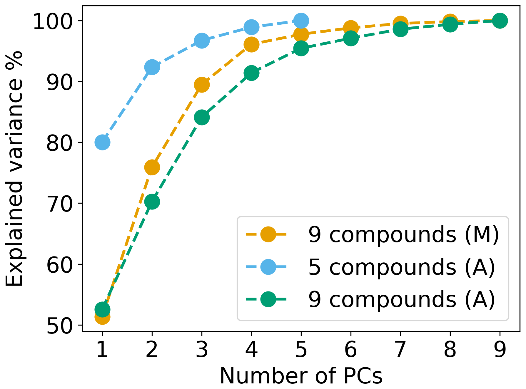
Figure 2Cumulative explained variance for automated (blue and green) and manual (orange) compound selection.
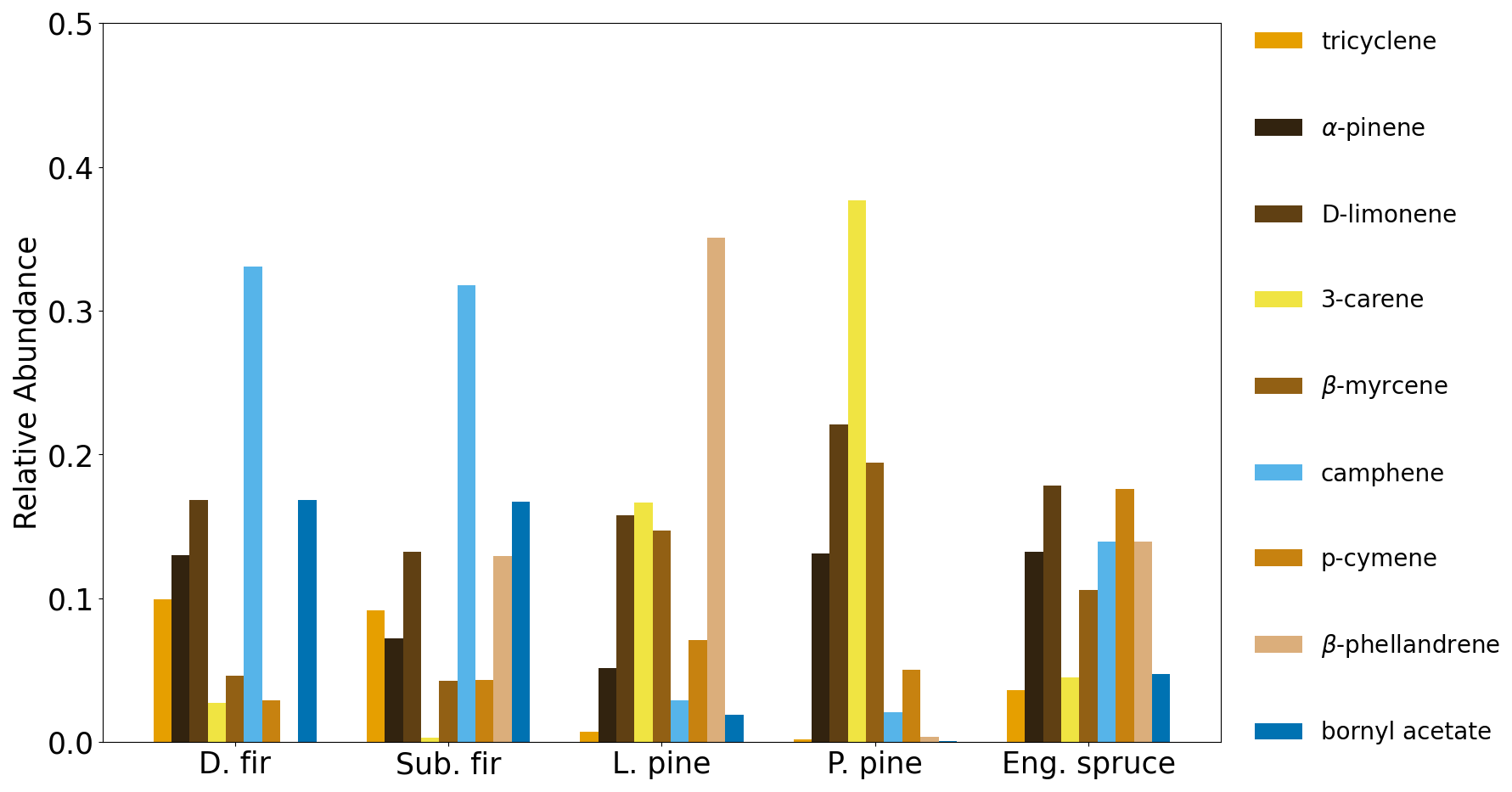
Figure 3Normalized emission ratio profiles for Douglas fir, subalpine fir, lodgepole pine, ponderosa pine and Engelmann spruce based on manual compound selection.
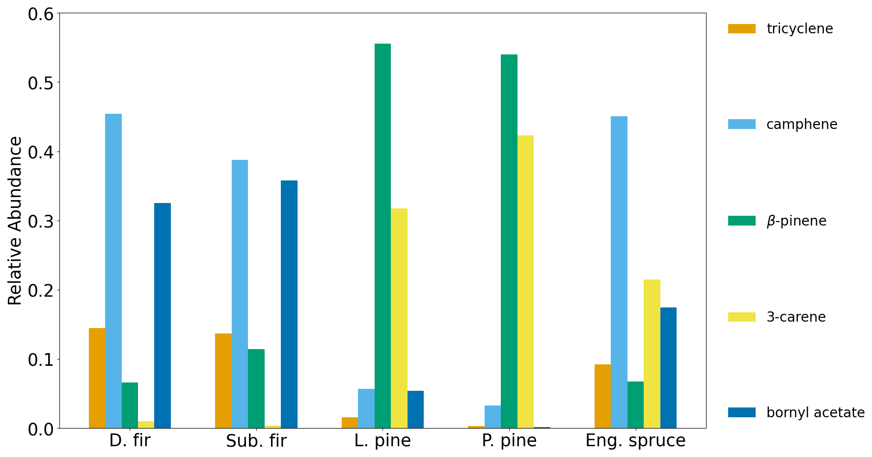
Figure 4Normalized emission ratio profiles for Douglas fir, subalpine fir, lodgepole pine, ponderosa pine and Engelmann spruce based on automated compound selection.
3.2.2 PCA and k-means clustering
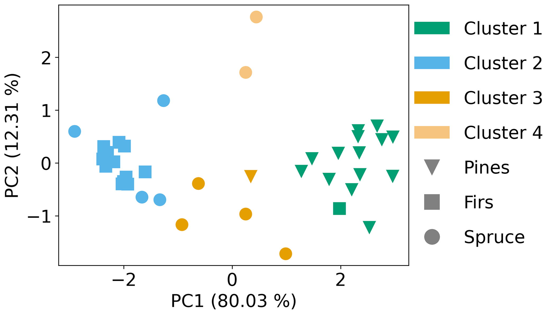
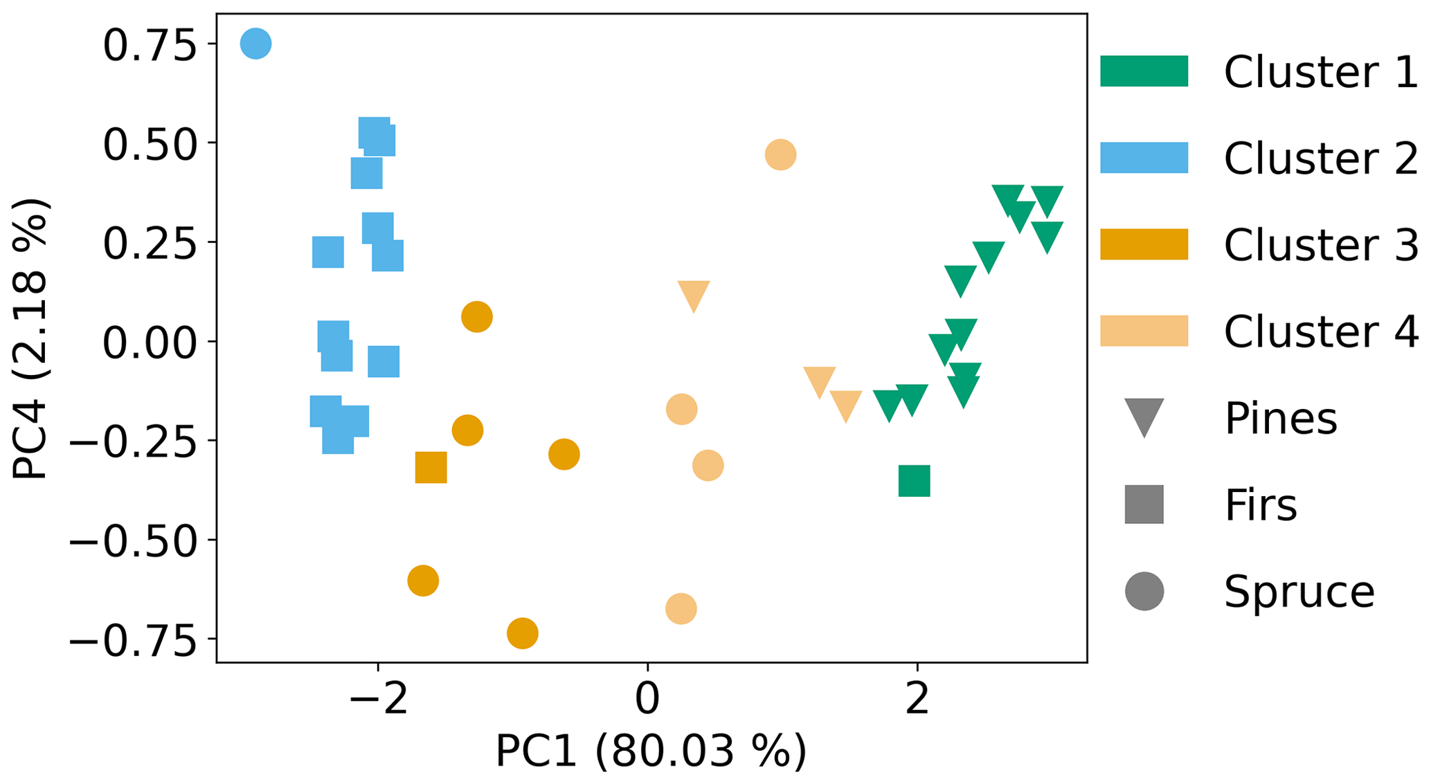
Following data preprocessing and feature selection, PCA was performed on the reduced data set (five compounds), followed by k-means clustering on two retained components (based on the explained variance metric, see Fig. 2). For k-means, the number of clusters was determined using the elbow plot method (Sect. 2.2.4). In Fig. 5, the TWSS is shown as a function of the number of clusters; the last inflection point occurs around four clusters (dark blue marker). The coupled PCA and k-means results are shown in Fig. 6. The clusters identified by the algorithm are differentiated by marker color while the fuel types are differentiated by marker shape. Cluster 1 included 15 out of 16 pine samples and one overlapping fir sample. Cluster 2 included 11 out of 13 fir samples and four overlapping spruce samples. Clusters 3 and 4 included the remaining six spruce samples, one overlapping pine sample and one overlapping fir sample. Generally, the algorithm resulted in adequate separation between firs and pines but poorer separation for spruce, for which four of 10 samples overlapped with another fuel family. Adding four more compounds reduced the variance explained by PC1 and PC2 from 92 % to less than 70 % and resulted in only a minor improvement in cluster separation (Fig. S6 in the Supplement). The difficulty that the algorithm encounters separating spruce effectively can be explained using the elbow plot (Fig. 5). The k-means algorithm identified four clusters as the optimum number, but the steep decrease in the total TWSS actually occurs between one and two total clusters. The TWSS decreases further between two and four, but to a lesser extent (shallower slope). The lesser decrease between two and four clusters indicates that the clustering algorithm had difficulty identifying clusters in the PCA space, which is then apparent in Fig. 6. From the normalized emission ratio profiles (Fig. 4), it can be seen that the spruce and fir samples have similar normalized emission ratios for tricyclene, camphene and β-pinene. This limits the ability to fully separate spruce and firs in the PCA space.
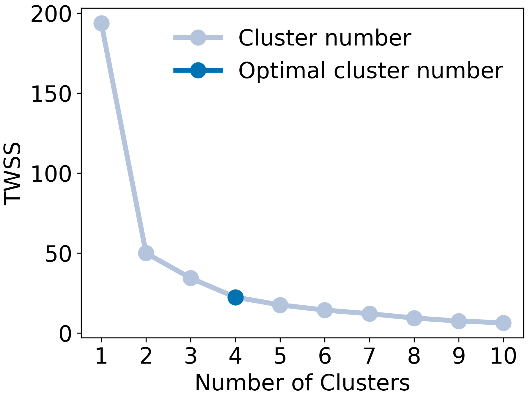
Figure 5Elbow plot for k-means clustering with automated compound selection for the PC1 and PC2 pair. The dark blue marker indicates the optimum number of clusters.
3.2.3 Beyond principal components one and two
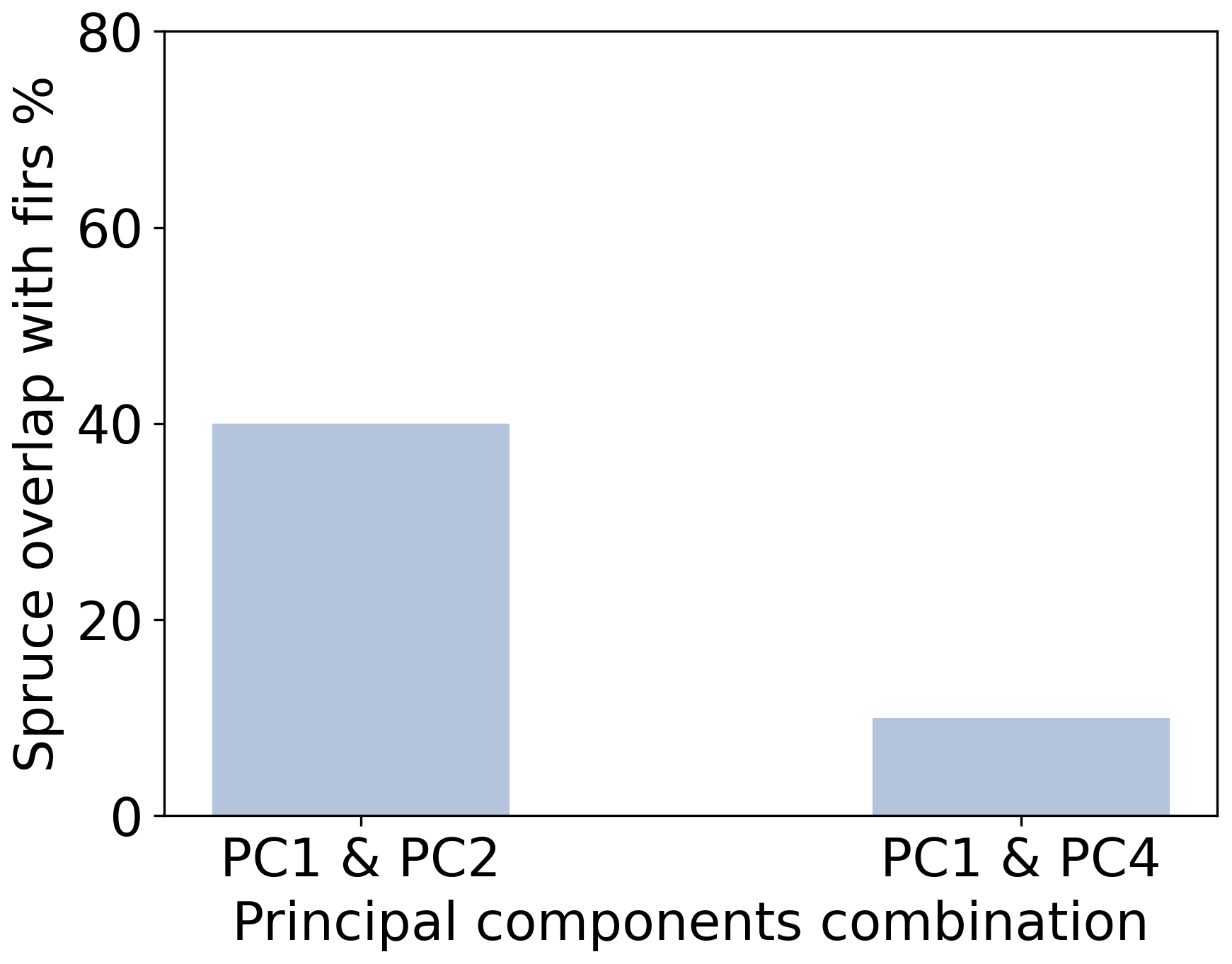
Thus far, only the first two PCs (from a total of five) had been used in the analysis, since they explained 92 % of the variance in the data set. Another 8 % was shared between PC3 and PC4, which could potentially provide better separation for the spruce samples. After testing PC1 with PC3 and PC1 with PC4, the combination of PC1 and PC4 was found to result in better performance of the PR algorithm. Though the optimal number of clusters for the PC1 and PC4 pair (Fig. 7) was the same as with the PC1 and PC2 pair, it was found at a lower TWSS, which is indicative of more dense clustering. Figure 8 shows the results for the PC1 and PC4 pair. Cluster 1 included 13 out of 16 pine samples and one overlapping fir sample. Cluster 2 included 11 out of 13 fir samples and only one overlapping spruce sample. Clusters 3 and 4 included 9 out of 10 spruce samples, one overlapping fir sample and three overlapping pine samples. With the PC1 and PC4 pair, spruce samples had 30 % less overlap with firs (Fig. 9), with only moderate losses in the separation between spruce and pines. These results demonstrate the ability of the PR algorithm to separate firs, pines and spruce in the smoke samples, with only two PCs accounting for most of the variance in the data set (PC1 and PC4 accounted for about 82 %).
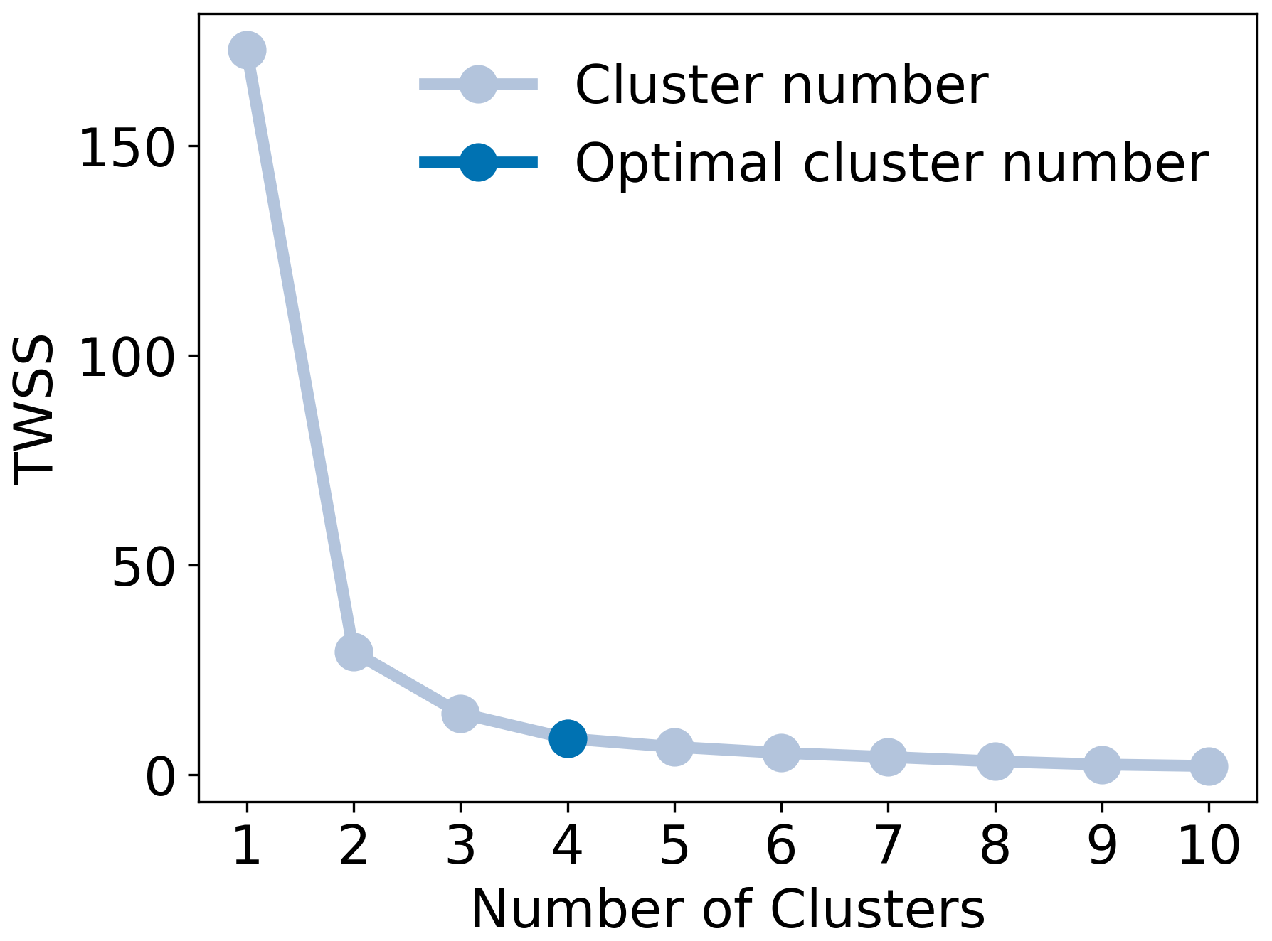
Figure 7Elbow plot for k-means clustering with automated compound selection for the PC1 and PC4 pair. The dark blue marker indicates the optimum number of clusters.
3.2.4 Mixed samples
The PR algorithm selected compounds that separated single-fuel smoke samples by the contribution of fuels categorized into three types (firs, pines and spruce). Before testing the algorithm on complex smoke samples, it was tested on the synthetic fuel mixtures described in Sect. 3.1. From the three 60/40 samples, only the fir/spruce synthetic mixture was clustered with the dominant fuel family (fir). The pine/spruce and pine/fir synthetic mixtures were clustered with spruce clusters 1 and 3, respectively (Fig. 10). The clustering of the pine/spruce synthetic mixture with spruce was marginal in the PCA space and was due to the scatter of the spruce samples rather than the similarity of the synthetic mixture with spruce. The clustering of the pine/fir mixture with spruce is more intuitive after comparing the normalized ER profiles (Fig. S7 in the Supplement), which show the similarities in the ER profiles for the pine/fir mixture and spruce. Figure 11 shows the PR results, including the 90/10 synthetic mixtures. Both samples were correctly clustered with their respective dominant fuel family. The synthetic mixture results suggest that the algorithm can select marker compounds that can differentiate fuel types, even when they are mixed in relatively even proportions (i.e., 60/40 pine/spruce and fir/spruce mixtures), but for some mixtures the differentiation might be poor (i.e., 60/40 pine/fir). Including more mixed fuel samples in the training and test sets would likely improve the separation of complex mixtures achieved using the PR algorithm.
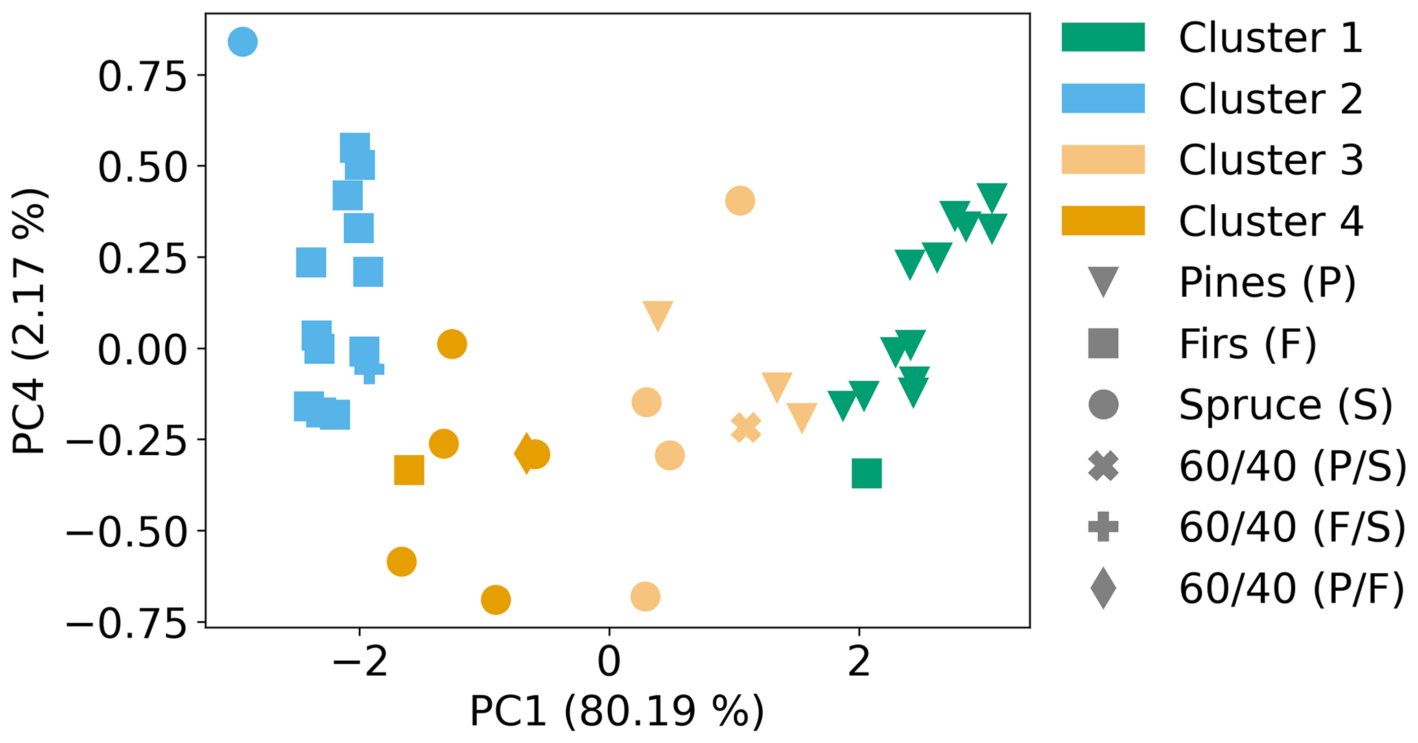
Figure 10PCA coupled with k-means clustering results for the PC1 and PC4 pair, including the 60 %/40 % synthetic mixtures.
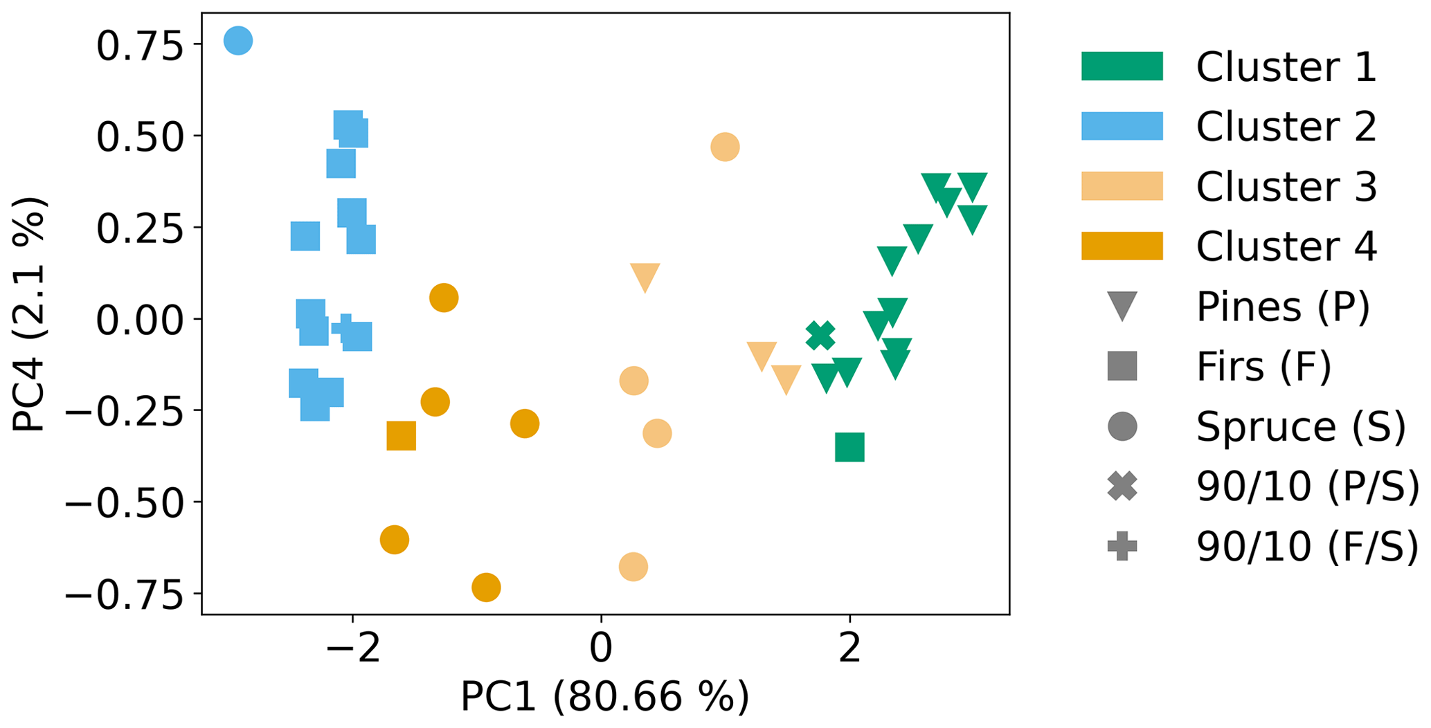
Figure 11PCA coupled with k-means clustering results for the PC1 and PC4 pair, including the 90 %/10 % synthetic mixtures.
3.3 Classification
3.3.1 Synthetic mixtures and FLAME-4 FL12 samples
After the pattern recognition, all 39 samples from the FIREX FL16 data set and the selected compounds in the form of the retained components (PC1 and PC4) were provided to the LDA algorithm for training. As described in Sect. 2.4, LDA provides class membership probability (Eq. 5). In this application, the probability score is related to the proximity of a sample to a class of samples (cluster) in the PCA space (Figs. 10 and 11), which is linked to its similarity with the emission profiles for the three fuel types (Fig. 4). The assignment of a sample to a class is based on the class with the highest probability, even when the probability is only marginally higher. For example, a sample with a pine probability score of 70 % or more will most likely be inside the pine cluster. Generally, samples with probability scores 60 % and higher are most likely in the cluster space of a fuel family. Samples with a probability score of 60 % or lower are more likely to be adjacent to one or more fuel families in the PCA space.
The classification algorithm was tested using the synthetic mixtures and FLAME-4 FL12 samples before testing using the BFRS field data. The classification results for the synthetic mixtures are shown in Fig. 12. Two of three 60/40 synthetic mixtures were classified correctly: pine/spruce and fir/spruce, with classification probabilities of 70 % and higher for the dominant fuel family. The 60/40 pine/fir synthetic mixture was classified as spruce. Its classification is a result of its clustering in the PCA space with spruce (Fig. 10), which is directly connected to its similarity with the spruce emission profile (Fig. S7). The two 90/10 synthetic mixtures, pine/spruce and fir/spruce, were correctly classified with classification probabilities of over 80 % for the dominant fuel family. Application of the classifier to the synthetic mixtures demonstrated that the mixtures can be correctly classified based on the dominant fuel family in mixed fuel samples (four of five mixtures); however, incorrect classification can occur when the mixed fuel emission profiles are similar to individual fuel emission profiles, resulting in poorer separation with PCA. The results of the classification algorithm for mixed samples can be improved in future work through expanded testing and training on a broader range of fuel types and relevant mixtures.
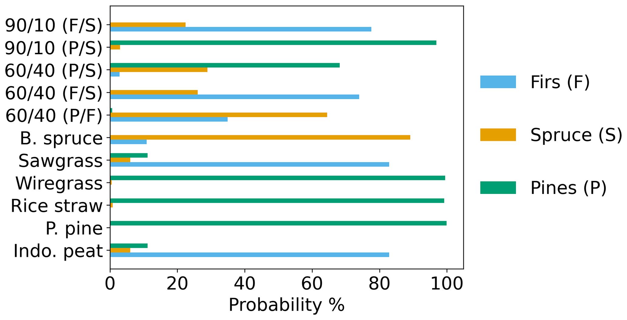
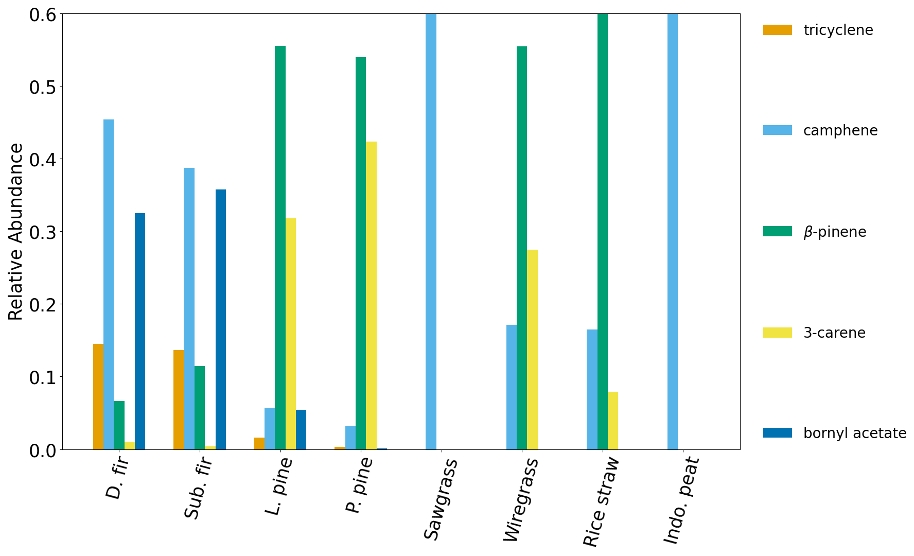
Figure 13Normalized emission ratio profiles for FIREX FL16 samples (pines and firs) and FLAME-4 FL12 samples (sawgrass, wiregrass, rice straw and Indonesian peat). The relative abundances of camphene and β-pinene in sawgrass, Indonesian peat and rice straw were ≥0.6, but, for figure clarity, the axis limits were not changed.
The classification results for the FLAME-4 FL12 samples are shown in Fig. 12. This data set included six fuel species (ponderosa pine, black spruce, Indonesian peat, rice straw, wiregrass and sawgrass), only one of which, ponderosa pine, was in the training set. Both the ponderosa pine and black spruce samples were classified correctly (Fig. 12), with classification probabilities of over 90 %. The Indonesian peat, rice straw, wiregrass and sawgrass samples were classified as firs or pines (Fig. 12), with classification probabilities of over 70 %. The classification algorithm evaluated partial similarity to only three options (pine, firs or spruce), none of which represent the fuel types of the four fuel species. Figure 13 shows the average normalized emission ratio profiles for pines and firs as well as Indonesian peat, rice straw, wiregrass and sawgrass. It can be seen that camphene is the only one of the five compounds that is present in the sawgrass and Indonesian peat samples, and thus these fuels were classified as firs, which also have a high relative abundance of camphene. Wiregrass and rice straw samples also include camphene, but have higher relative abundances of β-pinene and 3-carene, and thus were classified as pines, which also have higher relative abundances of these two compounds (Fig. 13). As illustrated by the application to the synthetic fuel mixtures, the performance of the classification algorithm can be improved in future work by expanding the range of fuel types and mixtures included in the training and test sets.
3.3.2 Blodgett samples
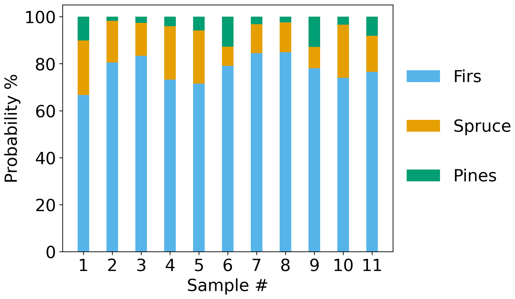
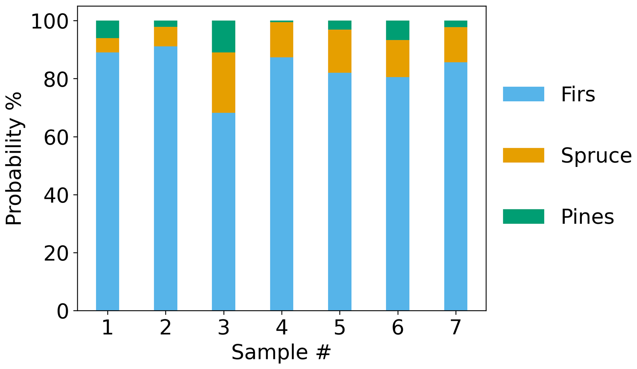
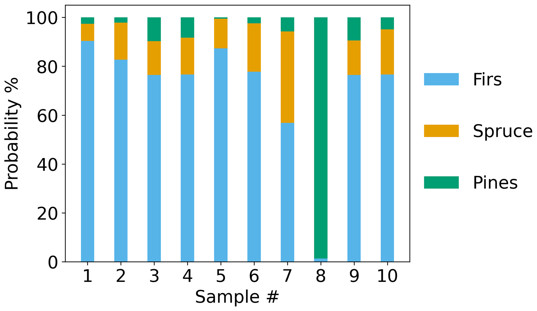
Figures 14–16 show the results of the classification algorithm applied to the BFRS samples from three different prescribed burn plots: 60, 340 and 400, the compositions of which are shown in Hatch et al. (2019) (Figs. S2–S4). Seven different fuel species were identified in the three burned plots: white fir, incense cedar, tanoak, sugar pine, ponderosa pine, Douglas fir and California black oak. Due to the heterogeneity of the fuels, and the influences of meteorology and sampling location, it was not possible to determine the relative contribution of each fuel species to each sample. Instead, the average overstory composition (Figs. S8–S11 in the Supplement) was used to determine likely influences from dominant sources close to each sampling location. For plot 60, sites 1 and 2 (Fig. S8), the main influence was from firs (47 %), followed by similar amounts of pines and incense cedar (25 % and 27 %), with no contribution from tanoak or California black oak. For plot 60, site 3 (Fig. S9), the main influence was from incense cedar (43 %), followed by firs (34 %), pines (26 %) and California black oak (10 %). For plot 340 (Fig. S10), the main influence was from firs (63 %), followed by pines (21 %), incense cedar (12 %) and tanoak and California black oak (2 %). Finally, for plot 400 (Fig. S11), the main influence was from firs (55 %), followed by pines (26 %) and incense cedar (18 %). The classification algorithm classified all samples from plots 60 (Fig. 14) and 340 (Fig. 15) as fir dominant. Nine out of 10 samples from plot 400 (Fig. 16) were classified as fir dominant, and one as pine dominant. While spruce was absent in the burned plots, all samples (with the exception of the pine-dominant sample in plot 400) had a higher classification probability for spruce than pines.
For plot 60, a total of 11 samples were collected: five samples in sites 1 and 2, which were fir dominant (Fig. S8), and six samples in site 3, which was incense cedar dominant (Fig. S9). For sites 1 and 2, the classifier results were reasonable based on the overstory composition, but for site 3, the classification results were inconclusive since no emission profiles were available for cedars. It is likely that incense cedar or the mixture of incense cedar with firs most closely resembles the fir emission profiles of the selected compounds and thus was classified as firs. For plots 340 and 400, the classification results – probabilities of 63 % for 340 and 55 % for 400 – are reasonable, given that 16 out of 17 samples are fir dominant (Figs. 15–16). The one sample that was classified as pines in plot 400 was most likely affected by ponderosa pine emissions during sampling. The composition plots in Hatch et al. (2019) show that one of the inventoried plots next to plot 400 (sites 1 and 2) had an average fractional overstory composition of more than 50 % ponderosa pine. The elevated probability of spruce despite its absence from all burned plots was likely an artifact of mixed smoke between pines and firs, which was also shown in the synthetic mixed sample PR and classification results. Among the three plots, pines and firs together account for more than 70 % of the overstory composition on average. Thus, the contributions from both firs and pines could lead to smoke mixtures that resemble the spruce emission profiles. Tanoak and California black oak (Figs. S8–S11) account for 2–10 % of the total contributions among the three plots. Due to insufficient emission data, their contributions to the smoke samples could not be evaluated, but given their low overstory contribution, it is likely that they did not influence the collected samples substantially. The results for the BFRS data showed that the laboratory-based emission profiles selected by the PR algorithm can be applied to smoke samples collected in the field, and can be used to identify dominant fuel sources, even in mixed smoke samples. While the algorithm has been tested and trained on only three fuel types, widespread application can be achieved with further training and testing using a more diverse set of compounds and a broader range of fuel types.
A supervised pattern recognition (PR) algorithm was developed and applied in this study to (1) differentiate sources/fuel types using NMOCs measured in smoke samples and selected with an ANOVA-based feature selection method and (2) train a classification algorithm to identify dominant sources/fuel types in smoke samples based on the unique speciation profiles identified by the PR algorithm. The PR algorithm was able to group five fuel species (Douglas and subalpine fir, ponderosa and loblolly pine, and Engelmann spruce) into three fuel types (pines, firs and spruce) with minimal overlap; only five of all 39 samples were grouped with types that were not representative of the fuel species. The separation was achieved using five monoterpenoids that the algorithm selected out of a pool of 93. Future work should include exploring how normality and heteroskedasticity, which are underlying assumptions for ANOVA, may be affecting separation. This can be achieved by using nonparametric tests that do not make assumptions about the underlying data distribution and are more robust than ANOVA in the presence of heteroskedasticity. The PR algorithm was tested with five synthetic mixtures, for which three of five (60/40 fir/spruce, 90/10 pine/spruce, and 90/10 fir/spruce) were successfully separated and clustered with their dominant family. The same synthetic mixtures were also tested using the classification algorithm, where four of five were classified correctly (60/40 pine/spruce, 60/40 fir/spruce, 90/10 pine/spruce and 90/10 fir/spruce). The application of the classification algorithm to the synthetic mixtures demonstrated that dominant source contributions could be identified in fuel mixtures. For the FLAME-4 FL12 samples, the classification algorithm correctly classified two of six samples (ponderosa pine and black spruce); these two samples were the only fuels represented by the three fuel types. For the BFRS field samples, based on the fractional overstory composition, the classification results were reasonable, with 27 out of 28 samples being classified as fir dominant and one sample as pine dominant. The incorrect classifications that occurred with the synthetic fuel mixture (60/40 pine/fir) and the FLAME-4 FL12 samples (Indonesian peat, rice straw, wiregrass and sawgrass) were due to the similarity or partial similarity of their emission profiles with the fuels used to train the classification model. This can be resolved in future applications by including more compounds and a broader range of fuel types, including in mixtures. This will also facilitate the use of this approach for identifying contributing fuels outside of western coniferous forests. The application of the PR algorithm is not confined to the analysis of biomass-burning emissions. In addition to linking NMOC speciation with fuel type, the PR algorithm can be used to link NMOC speciation with observational data relevant to air quality and climate, such as O3 and SOA levels.
The data used in the study can be found in the Supplement. Implementation scripts for the pattern recognition algorithm and the classification model are available through https://doi.org/10.5281/zenodo.6336170 Stamatis (2022).
The supplement related to this article is available online at: https://doi.org/10.5194/amt-15-2591-2022-supplement.
CS and KCB contributed equally to the paper; CS led the data analysis, data interpretation and paper preparation efforts; KCB led the conceptual design and editing of the paper.
The contact author has declared that neither they nor their co-author has any competing interests.
Publisher’s note: Copernicus Publications remains neutral with regard to jurisdictional claims in published maps and institutional affiliations.
The authors want to thank Lindsay Hatch for data acquisition and the processing of all FIREX FL16, FLAME-4 FL12 and BFRS samples; Ariel Roughton for the land cover analysis of the BFRS samples; Paul Van Rooy for discussions on the applicability of speciation profiles for data interpretation and smoke modeling; and Vanessa Selimovic for the CO data that were used for the ER calculations.
This research has been supported by the California Air Resources Board (grant no. 00010311) and the National Oceanic and Atmospheric Administration (grant nos. NA16OAR4310103 and NA17OAR4310007).
This paper was edited by Glenn Wolfe and reviewed by Santtu Mikkonen and two anonymous referees.
Abdi, H. and Williams, L. J.: Principal component analysis, WIREs Comput. Stat., 2, 433–459, https://doi.org/10.1002/wics.101, 2010. a
Alvarado, M. J. and Prinn, R. G.: Formation of ozone and growth of aerosols in young smoke plumes from biomass burning: 1. Lagrangian parcel studies, J. Geophys. Res.-Atmos., 114, D09306, https://doi.org/10.1029/2008JD011144, 2009. a
Andreae, M. O.: Emission of trace gases and aerosols from biomass burning – an updated assessment, Atmos. Chem. Phys., 19, 8523–8546, https://doi.org/10.5194/acp-19-8523-2019, 2019. a
Andreae, M. O., Browell, E. V., Garstang, M., Gregory, G. L., Harriss, R. C., Hill, G. F., Jacob, D. J., Pereira, M. C., Sachse, G. W., Setzer, A. W., Dias, P. L. S., Talbot, R. W., Torres, A. L., and Wofsy, S. C.: Biomass-burning emissions and associated haze layers over Amazonia, J. Geophys. Res.-Atmos., 93, 1509–1527, https://doi.org/10.1029/JD093iD02p01509, 1988. a
Chen, J., Anderson, K., Pavlovic, R., Moran, M. D., Englefield, P., Thompson, D. K., Munoz-Alpizar, R., and Landry, H.: The FireWork v2.0 air quality forecast system with biomass burning emissions from the Canadian Forest Fire Emissions Prediction System v2.03, Geosci. Model Dev., 12, 3283–3310, https://doi.org/10.5194/gmd-12-3283-2019, 2019. a
Dennison, P. E., Brewer, S. C., Arnold, J. D., and Moritz, M. A.: Large wildfire trends in the western United States, 1984–2011, Geophys. Res. Lett., 41, 2928–2933, https://doi.org/10.1002/2014GL059576, 2014. a, b
Dong, Y. and Peng, C.-Y. J.: Principled missing data methods for researchers, SpringerPlus, 2, 222, https://doi.org/10.1186/2193-1801-2-222, 2013. a, b
Elkan, C.: Using the Triangle Inequality to Accelerate K-Means, in: Proceedings of the Twentieth International Conference on International Conference on Machine Learning, ICML'03, p. 147–153, 21–24 August2003, Washington DC, USA, AAAI Press, 2003. a
Fu, P., Kawamura, K., and Barrie, L. A.: Photochemical and Other Sources of Organic Compounds in the Canadian High Arctic Aerosol Pollution during Winter−Spring, Environ. Sci. Technol., 43, 286–292, https://doi.org/10.1021/es803046q, 2009. a
Gewers, F. L., Ferreira, G. R., Arruda, H. F. D., Silva, F. N., Comin, C. H., Amancio, D. R., and Costa, L. D. F.: Principal Component Analysis: A Natural Approach to Data Exploration, ACM Comput. Surv., 54, 1–34, https://doi.org/10.1145/3447755, 2021. a, b
Goode, J. G., Yokelson, R. J., Ward, D. E., Susott, R. A., Babbitt, R. E., Davies, M. A., and Hao, W. M.: Measurements of excess O3, CO2, CO, CH4, C2H4, C2H2, HCN, NO, NH3, HCOOH, CH3COOH, HCHO, and CH3OH in 1997 Alaskan biomass burning plumes by airborne Fourier transform infrared spectroscopy (AFTIR), J. Geophys. Res.-Atmos., 105, 22147–22166, https://doi.org/10.1029/2000JD900287, 2000. a
Hastie, T., Tibshirani, R., and Friedman, J.: The Elements of Statistical Learning, Springer, New York, 145 pp., https://doi.org/10.1007/978-0-387-84858-7, 2009. a
Hatch, L. E., Luo, W., Pankow, J. F., Yokelson, R. J., Stockwell, C. E., and Barsanti, K. C.: Identification and quantification of gaseous organic compounds emitted from biomass burning using two-dimensional gas chromatography–time-of-flight mass spectrometry, Atmos. Chem. Phys., 15, 1865–1899, https://doi.org/10.5194/acp-15-1865-2015, 2015. a
Hatch, L. E., Yokelson, R. J., Stockwell, C. E., Veres, P. R., Simpson, I. J., Blake, D. R., Orlando, J. J., and Barsanti, K. C.: Multi-instrument comparison and compilation of non-methane organic gas emissions from biomass burning and implications for smoke-derived secondary organic aerosol precursors, Atmos. Chem. Phys., 17, 1471–1489, https://doi.org/10.5194/acp-17-1471-2017, 2017. a
Hatch, L. E., Rivas-Ubach, A., Jen, C. N., Lipton, M., Goldstein, A. H., and Barsanti, K. C.: Measurements of I/SVOCs in biomass-burning smoke using solid-phase extraction disks and two-dimensional gas chromatography, Atmos. Chem. Phys., 18, 17801–17817, https://doi.org/10.5194/acp-18-17801-2018, 2018. a
Hatch, L. E., Jen, C. N., Kreisberg, N. M., Selimovic, V., Yokelson, R. J., Stamatis, C., York, R. A., Foster, D., Stephens, S. L., Goldstein, A. H., and Barsanti, K. C.: Highly Speciated Measurements of Terpenoids Emitted from Laboratory and Mixed-Conifer Forest Prescribed Fires, Environ. Sci. Technol., 53, 9418–9428, https://doi.org/10.1021/acs.est.9b02612, 2019. a, b, c, d, e, f, g, h, i
Holder, A. L., Gullett, B. K., Urbanski, S. P., Elleman, R., O'Neill, S., Tabor, D., Mitchell, W., and Baker, K. R.: Emissions from prescribed burning of agricultural fields in the Pacific Northwest, Atmos. Environ., 166, 22–33, 2017. a
Hu, Y. Q., Fernandez-Anez, N., Smith, T. E. L., and Rein, G.: Review of emissions from smouldering peat fires and their contribution to regional haze episodes, Int. J. Wild. Fire, 27, 293–312, https://doi.org/10.1071/WF17084, 2018. a
Jaffe, D. A., O’Neill, S. M., Larkin, N. K., Holder, A. L., Peterson, D. L., Halofsky, J. E., and Rappold, A. G.: Wildfire and prescribed burning impacts on air quality in the United States, J. Air Waste Manage. Assoc., 70, 583–615, https://doi.org/10.1080/10962247.2020.1749731, 2020. a, b
Jain, A. K.: Data clustering: 50 years beyond K-means, Pattern Recogn. Lett., 31, 651–666, https://doi.org/10.1016/j.patrec.2009.09.011, award winning papers from the 19th International Conference on Pattern Recognition (ICPR), 2010. a, b
Jakobsen, J. C., Gluud, C., Wetterslev, J., and Winkel, P.: When and how should multiple imputation be used for handling missing data in randomised clinical trials – a practical guide with flowcharts, BMC Med. Res. Method., 17, 162, https://doi.org/10.1186/s12874-017-0442-1, 2017. a
Jen, C. N., Liang, Y., Hatch, L. E., Kreisberg, N. M., Stamatis, C., Kristensen, K., Battles, J. J., Stephens, S. L., York, R. A., Barsanti, K. C., and Goldstein, A. H.: High Hydroquinone Emissions from Burning Manzanita, Environ. Sci. Technol. Lett., 5, 309–314, https://doi.org/10.1021/acs.estlett.8b00222, 2018. a
Johnson, K. J. and Synovec, R. E.: Pattern recognition of jet fuels: comprehensive GC × GC with ANOVA-based feature selection and principal component analysis, Chemometr. Intell. Lab., 60, 225–237, https://doi.org/10.1016/S0169-7439(01)00198-8, fourth International Conference on Environ metrics and Chemometrics held in Las Vegas, NV, USA, 18–20 September 2000, 2002. a, b, c
Jolliffe, I.: Principal Component Analysis, Springer, New York, 188 pp., https://doi.org/10.1007/b98835, 2002. a
Keane, R. E. and Lutes, D.: First-Order Fire Effects Model (FOFEM), 1–5, Springer International Publishing, Cham, https://doi.org/10.1007/978-3-319-51727-8_74-1, 2018. a
Kochanski, A. K., Pardyjak, E. R., Stoll, R., Gowardhan, A., Brown, M. J., and Steenburgh, W. J.: One-Way Coupling of the WRF–QUIC Urban Dispersion Modeling System, J. Appl. Meteorol. Climatol., 54, 2119–2139, https://doi.org/10.1175/JAMC-D-15-0020.1, 2015. a
Koss, A. R., Sekimoto, K., Gilman, J. B., Selimovic, V., Coggon, M. M., Zarzana, K. J., Yuan, B., Lerner, B. M., Brown, S. S., Jimenez, J. L., Krechmer, J., Roberts, J. M., Warneke, C., Yokelson, R. J., and de Gouw, J.: Non-methane organic gas emissions from biomass burning: identification, quantification, and emission factors from PTR-ToF during the FIREX 2016 laboratory experiment, Atmos. Chem. Phys., 18, 3299–3319, https://doi.org/10.5194/acp-18-3299-2018, 2018. a, b
Lever, J., Krzywinski, M., and Altman, N.: Principal component analysis, Nat. Method., 14, 641–642, https://doi.org/10.1038/nmeth.4346, 2017. a
Lindaas, J., Pollack, I. B., Garofalo, L. A., Pothier, M. A., Farmer, D. K., Kreidenweis, S. M., Campos, T. L., Flocke, F., Weinheimer, A. J., Montzka, D. D., Tyndall, G. S., Palm, B. B., Peng, Q., Thornton, J. A., Permar, W., Wielgasz, C., Hu, L., Ottmar, R. D., Restaino, J. C., Hudak, A. T., Ku, I.-T., Zhou, Y., Sive, B. C., Sullivan, A., Collett Jr., J. L., and Fischer, E. V.: Emissions of Reactive Nitrogen From Western U.S. Wildfires During Summer 2018, J. Geophys. Res.-Atmos., 126, e2020JD032657, https://doi.org/10.1029/2020JD032657, 2021. a
Liu, X., Huey, L. G., Yokelson, R. J., Selimovic, V., Simpson, I. J., Müller, M., Jimenez, J. L., Campuzano-Jost, P., Beyersdorf, A. J., Blake, D. R., Butterfield, Z., Choi, Y., Crounse, J. D., Day, D. A., Diskin, G. S., Dubey, M. K., Fortner, E., Hanisco, T. F., Hu, W., King, L. E., Kleinman, L., Meinardi, S., Mikoviny, T., Onasch, T. B., Palm, B. B., Peischl, J., Pollack, I. B., Ryerson, T. B., Sachse, G. W., Sedlacek, A. J., Shilling, J. E., Springston, S., St. Clair, J. M., Tanner, D. J., Teng, A. P., Wennberg, P. O., Wisthaler, A., and Wolfe, G. M.: Airborne measurements of western U.S. wildfire emissions: Comparison with prescribed burning and air quality implications, J. Geophys. Res.-Atmos., 122, 6108–6129, https://doi.org/10.1002/2016JD026315, 2017. a, b
McKenzie, D., O’Neill, S. M., Larkin, N. K., and Norheim, R. A.: Integrating models to predict regional haze from wildland fire, Ecol. Modell., 199, 278–288, https://doi.org/10.1016/j.ecolmodel.2006.05.029, 2006. a
McMeeking, G. R., Kreidenweis, S. M., Carrico, C. M., Lee, T., Collett Jr., J. L., and Malm, W. C.: Observations of smoke-influenced aerosol during the Yosemite Aerosol Characterization Study: Size distributions and chemical composition, J. Geophys. Res.-Atmos., 110, D09206, https://doi.org/10.1029/2004JD005389, 2005. a
McNeish, D.: Missing data methods for arbitrary missingness with small samples, J. Appl. Stat., 44, 24–39, https://doi.org/10.1080/02664763.2016.1158246, 2017. a
Miller, J. D., Safford, H. D., Crimmins, M., and Thode, A. E.: Quantitative Evidence for Increasing Forest Fire Severity in the Sierra Nevada and Southern Cascade Mountains, California and Nevada, USA, Ecosystems, 12, 16–32, https://doi.org/10.1007/s10021-008-9201-9, 2009. a, b
Nelson, K. J., Connot, J., Peterson, B., and Martin, C.: The LANDFIRE Refresh Strategy: Updating the National Dataset, Fire Ecol., 9, 80–101, https://doi.org/10.4996/fireecology.0902080, 2013. a
Ottmar, R.: Consume 3.0 – A Software Tool for Computing Fuel Consumption, Fire Sci. Brief, p. 6, https://www.firescience.gov/projects/briefs/98-1-9-06_FSBrief55.pdf (last access: 6 April 2022), 2009. a
Park, R. J., Jacob, D. J., Kumar, N., and Yantosca, R. M.: Regional visibility statistics in the United States: Natural and transboundary pollution influences, and implications for the Regional Haze Rule, Atmos. Environ., 40, 5405–5423, 2006. a
Pavlovic, R., Chen, J., Anderson, K., Moran, M. D., Beaulieu, P.-A., Davignon, D., and Cousineau, S.: The FireWork air quality forecast system with near-real-time biomass burning emissions: Recent developments and evaluation of performance for the 2015 North American wildfire season, J. Air Waste Manage. Assoc., 66, 819–841, https://doi.org/10.1080/10962247.2016.1158214, 2016. a
Pedregosa, F., Varoquaux, G., Gramfort, A., Michel, V., Thirion, B., Grisel, O., Blondel, M., Prettenhofer, P., Weiss, R., Dubourg, V., Vanderplas, J., Passos, A., Cournapeau, D., Brucher, M., Perrot, M., and Duchesnay, E.: Scikit-learn: Machine Learning in Python, J. Machine Learn. Res., 12, 2825–2830, 2011. a
Permar, W., Wang, Q., Selimovic, V., Wielgasz, C., Yokelson, R. J., Hornbrook, R. S., Hills, A. J., Apel, E. C., Ku, I.-T., Zhou, Y., Sive, B. C., Sullivan, A. P., Collett Jr., J. L., Campos, T. L., Palm, B. B., Peng, Q., Thornton, J. A., Garofalo, L. A., Farmer, D. K., Kreidenweis, S. M., Levin, E. J. T., DeMott, P. J., Flocke, F., Fischer, E. V., and Hu, L.: Emissions of Trace Organic Gases From Western U.S. Wildfires Based on WE-CAN Aircraft Measurements, J. Geophys. Res.-Atmos., 126, e2020JD033838, https://doi.org/10.1029/2020JD033838, 2021. a
Prichard, S., Larkin, N. S., Ottmar, R., French, N. H., Baker, K., Brown, T., Clements, C., Dickinson, M., Hudak, A., Kochanski, A., Linn, R., Liu, Y., Potter, B., Mell, W., Tanzer, D., Urbanski, S., and Watts, A.: The Fire and Smoke Model Evaluation Experiment – A Plan for Integrated, Large Fire – Atmosphere Field Campaigns, Atmosphere, 10, 2, https://doi.org/10.3390/atmos10020066, 2019. a
Prichard, S. J., O'Neill, S. M., Eagle, P., Andreu, A. G., Drye, B., Dubowy, J., Urbanski, S., and Strand, T. M.: Wildland fire emission factors in North America: synthesis of existing data, measurement needs and management applications, Int. J. Wildl. Fire, 29, 132–147, https://doi.org/10.1071/WF19066, 2020. a, b
Reeves, M. C., Ryan, K. C., Rollins, M. G., and Thompson, T. G.: Spatial fuel data products of the LANDFIRE Project, Int. J. Wildl. Fire, 18, 250–267, https://doi.org/10.1071/WF08086, 2009. a
Sekimoto, K., Koss, A. R., Gilman, J. B., Selimovic, V., Coggon, M. M., Zarzana, K. J., Yuan, B., Lerner, B. M., Brown, S. S., Warneke, C., Yokelson, R. J., Roberts, J. M., and de Gouw, J.: High- and low-temperature pyrolysis profiles describe volatile organic compound emissions from western US wildfire fuels, Atmos. Chem. Phys., 18, 9263–9281, https://doi.org/10.5194/acp-18-9263-2018, 2018. a, b
Selimovic, V., Yokelson, R. J., Warneke, C., Roberts, J. M., de Gouw, J., Reardon, J., and Griffith, D. W. T.: Aerosol optical properties and trace gas emissions by PAX and OP-FTIR for laboratory-simulated western US wildfires during FIREX, Atmos. Chem. Phys., 18, 2929–2948, https://doi.org/10.5194/acp-18-2929-2018, 2018. a, b, c
Simoneit, B. R.: Biomass burning – a review of organic tracers for smoke from incomplete combustion, Appl. Geochem., 17, 129–162, 2002. a
Simpson, I. J., Akagi, S. K., Barletta, B., Blake, N. J., Choi, Y., Diskin, G. S., Fried, A., Fuelberg, H. E., Meinardi, S., Rowland, F. S., Vay, S. A., Weinheimer, A. J., Wennberg, P. O., Wiebring, P., Wisthaler, A., Yang, M., Yokelson, R. J., and Blake, D. R.: Boreal forest fire emissions in fresh Canadian smoke plumes: C1-C10 volatile organic compounds (VOCs), CO2, CO, NO2, NO, HCN and CH3CN, Atmos. Chem. Phys., 11, 6445–6463, https://doi.org/10.5194/acp-11-6445-2011, 2011. a
Stamatis, C.: christos-stamatis/supervised_pattern_recognition: 70(v3.0), Zenodo [code], https://doi.org/10.5281/zenodo.6336170, 2022. a
Stockwell, C. E., Yokelson, R. J., Kreidenweis, S. M., Robinson, A. L., DeMott, P. J., Sullivan, R. C., Reardon, J., Ryan, K. C., Griffith, D. W. T., and Stevens, L.: Trace gas emissions from combustion of peat, crop residue, domestic biofuels, grasses, and other fuels: configuration and Fourier transform infrared (FTIR) component of the fourth Fire Lab at Missoula Experiment (FLAME-4), Atmos. Chem. Phys., 14, 9727–9754, https://doi.org/10.5194/acp-14-9727-2014, 2014. a, b, c, d, e, f
Stockwell, C. E., Veres, P. R., Williams, J., and Yokelson, R. J.: Characterization of biomass burning emissions from cooking fires, peat, crop residue, and other fuels with high-resolution proton-transfer-reaction time-of-flight mass spectrometry, Atmos. Chem. Phys., 15, 845–865, https://doi.org/10.5194/acp-15-845-2015, 2015. a, b, c
Urbanski, S.: Wildland fire emissions, carbon, and climate: Emission factors, Forest Ecol. Manage., 317, 51–60, 2014. a
Urbanski, S. P.: Combustion efficiency and emission factors for wildfire-season fires in mixed conifer forests of the northern Rocky Mountains, US, Atmos. Chem. Phys., 13, 7241–7262, https://doi.org/10.5194/acp-13-7241-2013, 2013. a
Urbanski, S. P., Hao, W. M., and Baker, S.: Chapter 4 Chemical Composition of Wildland Fire Emissions, Vol. 8, Wildland Fires and Air Pollution, pp. 79–107, Elsevier, 2008. a
Vogelmann, J. E., Kost, J. R., Tolk, B., Howard, S., Short, K., Chen, X., Huang, C., Pabst, K., and Rollins, M. G.: Monitoring Landscape Change for LANDFIRE Using Multi-Temporal Satellite Imagery and Ancillary Data, IEEE J. Sel. Top. Appl., 4, 252–264, https://doi.org/10.1109/JSTARS.2010.2044478, 2011. a
Wan, X., Kawamura, K., Ram, K., Kang, S., Loewen, M., Gao, S., Wu, G., Fu, P., Zhang, Y., Bhattarai, H., and Cong, Z.: Aromatic acids as biomass-burning tracers in atmospheric aerosols and ice cores: A review, Environ. Pollut., 247, 216–228, 2019. a
Ward, D. E. and Hardy, C. C.: Smoke emissions from wildland fires, Environ. Int., 17, 117–134, 1991. a
Welke, J. E., Manfroi, V., Zanus, M., Lazzarotto, M., and Alcaraz Zini, C.: Differentiation of wines according to grape variety using multivariate analysis of comprehensive two-dimensional gas chromatography with time-of-flight mass spectrometric detection data, Food Chem., 141, 3897–3905, https://doi.org/10.1016/j.foodchem.2013.06.100, 2013. a, b, c
Westerling, A. L., Hidalgo, H. G., Cayan, D. R., and Swetnam, T. W.: Warming and Earlier Spring Increase Western U.S. Forest Wildfire Activity, Science, 313, 940–943, https://doi.org/10.1126/science.1128834, 2006. a
Yokelson, R. J., Goode, J. G., Ward, D. E., Susott, R. A., Babbitt, R. E., Wade, D. D., Bertschi, I., Griffith, D. W. T., and Hao, W. M.: Emissions of formaldehyde, acetic acid, methanol, and other trace gases from biomass fires in North Carolina measured by airborne Fourier transform infrared spectroscopy, J. Geophys. Res.-Atmos., 104, 30109–30125, https://doi.org/10.1029/1999JD900817, 1999. a
Yokelson, R. J., Burling, I. R., Gilman, J. B., Warneke, C., Stockwell, C. E., de Gouw, J., Akagi, S. K., Urbanski, S. P., Veres, P., Roberts, J. M., Kuster, W. C., Reardon, J., Griffith, D. W. T., Johnson, T. J., Hosseini, S., Miller, J. W., Cocker III, D. R., Jung, H., and Weise, D. R.: Coupling field and laboratory measurements to estimate the emission factors of identified and unidentified trace gases for prescribed fires, Atmos. Chem. Phys., 13, 89–116, https://doi.org/10.5194/acp-13-89-2013, 2013. a, b
Zangrando, R., Barbaro, E., Zennaro, P., Rossi, S., Kehrwald, N. M., Gabrieli, J., Barbante, C., and Gambaro, A.: Molecular Markers of Biomass Burning in Arctic Aerosols, Environ. Sci. Technol., 47, 8565–8574, https://doi.org/10.1021/es400125r, 2013. a
Zhang, Q., Jimenez, J. L., Canagaratna, M. R., Allan, J. D., Coe, H., Ulbrich, I., Alfarra, M. R., Takami, A., Middlebrook, A. M., Sun, Y. L., Dzepina, K., Dunlea, E., Docherty, K., DeCarlo, P. F., Salcedo, D., Onasch, T., Jayne, J. T., Miyoshi, T., Shimono, A., Hatakeyama, S., Takegawa, N., Kondo, Y., Schneider, J., Drewnick, F., Borrmann, S., Weimer, S., Demerjian, K., Williams, P., Bower, K., Bahreini, R., Cottrell, L., Griffin, R. J., Rautiainen, J., Sun, J. Y., Zhang, Y. M., and Worsnop, D. R.: Ubiquity and dominance of oxygenated species in organic aerosols in anthropogenically-influenced Northern Hemisphere midlatitudes, Geophys. Res. Lett., 34, L13801, https://doi.org/10.1029/2007GL029979, 2007. a
Zhang, Y., Kong, S., Sheng, J., Zhao, D., Ding, D., Yao, L., Zheng, H., Wu, J., Cheng, Y., Yan, Q., Niu, Z., Zheng, S., Wu, F., Yan, Y., Liu, D., and Qi, S.: Real-time emission and stage-dependent emission factors/ratios of specific volatile organic compounds from residential biomass combustion in China, Atmos. Res., 248, 105189, 2021. a
Ziółkowska, A., Wąsowicz, E., and Jeleń, H. H.: Differentiation of wines according to grape variety and geographical origin based on volatiles profiling using SPME-MS and SPME-GC/MS methods, Food Chem., 213, 714–720, https://doi.org/10.1016/j.foodchem.2016.06.120, 2016. a, b