Synergy of Using Nadir and Limb Instruments for Tropospheric Ozone Monitoring (SUNLIT)

Satellite measurements in nadir and limb viewing geometry provide a complementary view of the atmosphere. An effective combination of the limb and nadir measurements can give new information about atmospheric composition. In this work, we present tropospheric ozone column datasets that have been created using a combination of total ozone columns from OMI (Ozone Monitoring Instrument) and TROPOMI (TROPOspheric Monitoring Instrument) with stratospheric ozone column datasets from several available limb-viewing instruments: MLS (Microwave Limb Sounder), OSIRIS (Optical Spectrograph and InfraRed Imaging System), MIPAS (Michelson Interferometer for Passive Atmospheric Sounding), SCIAMACHY (SCanning Imaging Spectrometer for Atmospheric CHartographY), OMPS-LP (Ozone Mapping and Profiles Suite – Limb Profiler), and GOMOS (Global Ozone Monitoring by Occultation of Stars).

We have developed further the methodological aspects of the assessment of tropospheric ozone using the residual method supported by simulations with the chemistry transport model SILAM (System for Integrated modeLling of Atmospheric coMposition). It has been shown that the accurate assessment of ozone in the upper troposphere and the lower stratosphere (UTLS) is of high importance for detecting the ground-level ozone patterns.

The stratospheric ozone column is derived from a combination of ozone profiles from several satellite instruments in limb-viewing geometry. We developed a method for the data homogenization, which includes the removal of biases and a posteriori estimation of random uncertainties, thus making the data from different instruments compatible with each other. The high-horizontal- and vertical-resolution dataset of ozone profiles is created via interpolation of the limb profiles from each day to a $\mathrm{1}{}^{\circ }\times \mathrm{1}{}^{\circ }$ horizonal grid. A new kriging-type interpolation method, which takes into account data uncertainties and the information about natural ozone variations from the SILAM-adjusted ozone field, has been developed. To mitigate the limited accuracy and coverage of the limb profile data in the UTLS, a smooth transition to the model data is applied below the tropopause. This allows for the estimation of the stratospheric ozone column with full coverage of the UTLS. The derived ozone profiles are in very good agreement with collocated ozonesonde measurements.

The residual method was successfully applied to OMI and TROPOMI clear-sky total ozone data in combination with the stratospheric ozone column from the developed high-resolution limb profile dataset. The resulting tropospheric ozone column is in very good agreement with other satellite data. The global distributions of tropospheric ozone exhibit enhancements associated with the regions of high tropospheric ozone production.

The main datasets created are (i) a monthly $\mathrm{1}{}^{\circ }\times \mathrm{1}{}^{\circ }$ global tropospheric ozone column dataset (from ground to 3 km below the tropopause) using OMI and limb instruments, (ii) a monthly $\mathrm{1}{}^{\circ }\times \mathrm{1}{}^{\circ }$ global tropospheric ozone column dataset using TROPOMI and limb instruments, and (iii) a daily $\mathrm{1}{}^{\circ }\times \mathrm{1}{}^{\circ }$ interpolated stratospheric ozone column from limb instruments.

Other datasets, which are created as an intermediate step of creating the tropospheric ozone column data, are (i) a daily $\mathrm{1}{}^{\circ }\times \mathrm{1}{}^{\circ }$ clear-sky and total ozone column from OMI and TROPOMI, (ii) a daily $\mathrm{1}{}^{\circ }\times \mathrm{1}{}^{\circ }$ homogenized and interpolated dataset of ozone profiles from limb instruments, and (iii) a daily $\mathrm{1}{}^{\circ }\times \mathrm{1}{}^{\circ }$ dataset of ozone profiles from SILAM simulations with adjustment to satellite data.

These datasets can be used in various studies related to variability and trends in ozone distributions in both the troposphere and the stratosphere. The datasets are processed from the beginning of OMI and TROPOMI measurements until December 2020 and are planned to be regularly extended in the future.

1 Introduction

Detailed information about the tropospheric ozone is of high importance because the impact of its changes is one of the major environmental concerns. Upper-tropospheric ozone is an important greenhouse gas which contributes to global warming. Tropospheric ozone is also a pollutant affecting air quality. It is responsible for respiratory diseases in humans, leads to premature mortality, and causes damage to crops and ecosystems (e.g., Jacobson, 2012; Lippmann, 1991). It was shown that the amount of tropospheric ozone increased globally during the 20th century due to enhanced emissions of anthropogenic precursors (e.g., Marenco et al., 1994; Shindell et al., 2006).

Satellite measurements in nadir and limb viewing geometry provide a complementary view of the atmosphere. These two measurement systems have their own advantages and limitations. The nadir-looking instruments have a good horizontal resolution; they are good in retrievals of total columns, while their vertical resolution is limited. The measurements in the limb-viewing geometry have usually a good vertical resolution, but their horizontal resolution is limited by the spatial sampling. In particular, the horizontal resolution along the line of sight is limited by the effective horizontal length of interaction with the atmosphere (a few hundreds of kilometers). The limb profilers allow for a good quality of trace gas retrievals in the stratosphere, while the retrievals from limb instruments in the troposphere are often problematic due to the low signal-to-noise ratio and presence of clouds. (Note that the presence of clouds causes also problems for the nadir measurements.) An effective combination of the limb and nadir measurements of atmospheric composition can provide additional information about atmospheric composition. Successful examples of such a combination are tropospheric ozone datasets obtained by subtracting stratospheric columns from the total ozone columns for OMI (Ozone Monitoring Instrument) nadir and MLS (Microwave Limb Sounder) profile measurements (Ziemke et al., 2006), as well as for SCIAMACHY (SCanning Imaging Spectrometer for Atmospheric CHartographY) limb–nadir matching measurements (Ebojie et al., 2016).

The retrieval of tropospheric ozone from purely nadir-looking instruments is a challenging, strongly ill-posed problem. Therefore several approaches have been developed: (1) using the spectral information in the nadir satellite measurements (nadir profile retrievals; Kroon et al., 2011; Liu et al., 2010a, b; Mielonen et al., 2015), (2) the convective cloud differential (CCD) method applied in the tropics (Heue et al., 2016; Leventidou et al., 2016; Ziemke et al., 1998), and (3) via subtraction of the stratospheric column from an external source from the total ozone column (the residual method). The first study with the residual method was performed in the late 1980s by Fishman and Larsen (1987), who subtracted SAGE (Stratospheric Aerosol and Gas Experiment) stratospheric ozone from total ozone columns by TOMS (Total Ozone Mapping Spectrometer). Aside from calibration issues when using a combination of TOMS and SAGE measurements, there was also a serious constraint in producing global data with adequate temporal and spatial coverage due to sparse coverage by the SAGE solar occultation measurements. Several other residual-based approaches have been developed over the years, with combinations of TOMS and MLS on UARS (Upper Atmosphere Research Satellite; Fishman et al., 1990) and OMI and MLS (Schoeberl et al., 2007; Ziemke et al., 2006, 2011).

The main problems associated with the tropospheric ozone retrievals from nadir and limb measurements are (i) necessity of data calibration and (ii) usually insufficient horizontal coverage of limb profile measurements. In order to get the stratospheric ozone field with high horizontal resolution, a 2D interpolation (Ziemke et al., 2006) or wind trajectory scheme (Schoeberl et al., 2007) is used.

The satellite measurements of total ozone by TROPOMI (TROPOspheric Monitoring Instrument) on Sentinel-5P open new possibilities for monitoring atmospheric pollutants from space because of their unprecedented horizontal resolution.

The main aim of our work is the further development of the methods for the assessment of tropospheric ozone using synergy of limb and nadir measurements and applying them to measurements by TROPOMI on Sentinel-5P and OMI on Aura. The novelty of the approach is in the combination of the measurements from several satellite instruments in limb-viewing geometry for the stratospheric ozone column dataset. In addition, we have performed extensive sensitivity studies using simulations with the chemistry transport model (CTM) SILAM (System for Integrated modeLling of Atmospheric coMposition; Sofiev et al., 2015, 2020).

This paper presents the description of the methods developed within the ESA project SUNLIT (Synergy of Using Nadir and Limb Instruments for Tropospheric Ozone Monitoring) and shows some illustrative examples of the created datasets. The methods being developed in this study have a focus on optimizing monthly-averaged tropospheric ozone values, which are mainly interesting for long-term studies and climatological analysis. The paper is organized as follows. Section 2 describes the satellite datasets and the CTM SILAM. Section 3 is dedicated to feasibility studies on retrievals of tropospheric ozone by the residual method, which have been performed using simulations with SILAM. Section 4 describes the retrieval method for the tropospheric ozone column developed in the SUNLIT project. Examples of data and some validation results are shown in Sect. 5. A summary (Sect. 6) concludes the paper. Additional illustrations are provided in the Supplement.

2 Data and the chemistry transport model

2.1 Total ozone column from nadir satellite instruments

In our analyses we use total column ozone data from OMI on Aura (https://aura.gsfc.nasa.gov/omi.html, last access: 6 April 2022; Levelt et al., 2018) and TROPOMI on Sentinel-5P (http://www.tropomi.eu, last access: 6 April 2022; https://sentinel.esa.int/web/sentinel/missions/sentinel-5p, last access: 6 April 2022; Veefkind et al., 2012). OMI and TROPOMI are in sun-synchronous orbits and provide the information at about the same local time (13:30 and 13:45). OMI has been operating since 2004, and its data have been used in different applications including the evaluation of trends (Levelt et al., 2018). The OMI ground pixel size is 13 km×25 km. TROPOMI has been operating since 2017. It has a very fine spatial resolution with the ground pixel size 3.5 km×7 km before August 2019 and 3.5 km×5.5 km afterwards.

In our work, we use the Level 2 OMI and TROPOMI total ozone columns retrieved with the same GODFIT v4.0 processor developed in the ESA Ozone_cci project (Lerot et al., 2014). Total ozone columns are derived using a non-linear minimization procedure of the differences between measured and modeled sun-normalized radiances in the ozone Huggins bands (fitting window: 325–335 nm). The typical random uncertainties of total column data, as estimated by the retrieval algorithm, are in the range of 0.5–5 DU for OMI and 0.5–2 DU for TROPOMI (Lerot et al., 2014; Sofieva et al., 2021).

2.2 Ozone profiles from limb satellite measurements

We use the data from several limb and occultation satellite instruments. Three of them – MIPAS (Michelson Interferometer for Passive Atmospheric Sounding), SCIAMACHY, and GOMOS (Global Ozone Monitoring by Occultation of Stars) – operated on Envisat (Environmental Satellite) in 2002–2012. Three other limb instruments are still operational: OSIRIS (Optical Spectrograph and InfraRed Imaging System) on Odin, MLS on Aura, and OMPS-LP (Ozone Mapping and Profiles Suite – Limb Profiler) on Suomi-NPP (National Polar-orbiting Partnership).

The information about the ozone profile data is collected in Table 1. All these satellites are in sun-synchronous orbits so that the measurements are performed in nearly the same local overpass time, which is instrument-specific. MLS and OMPS measurements are performed at local times close to OMI and TROPOMI measurements, which is advantageous for the proposed application. The abovementioned limb instruments provide ozone profiles with a vertical resolution of 2–4 km and random uncertainties of 1 %–10 % in the stratosphere (see Table 1 for more details). The horizontal resolution associated with the limb-profile measurement technique is 200–400 km along the line of sight. The selected limb instruments provide from ∼100 to ∼3500 profiles per day (Table 1), which are spaced uniformly in longitudinal direction according to satellite orbits (typical daily sampling patterns are illustrated in Fig. 7 below).

Table 1 Information about the datasets used in the analyses.

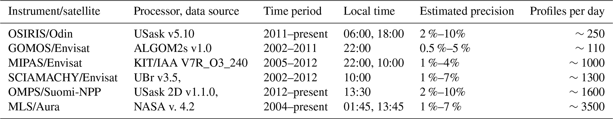
The accuracy and data coverage are lower in the upper troposphere and the lower stratosphere (UTLS) than in the middle stratosphere (Fig. 1). For limb-viewing satellite measurements, retrievals in the UTLS are challenging due to the presence of clouds and lower signal-to-noise ratio. The average estimated random uncertainties are in the range 5 %–30 %. Not all ozone profiles cover fully the UTLS region (Fig. 1c).

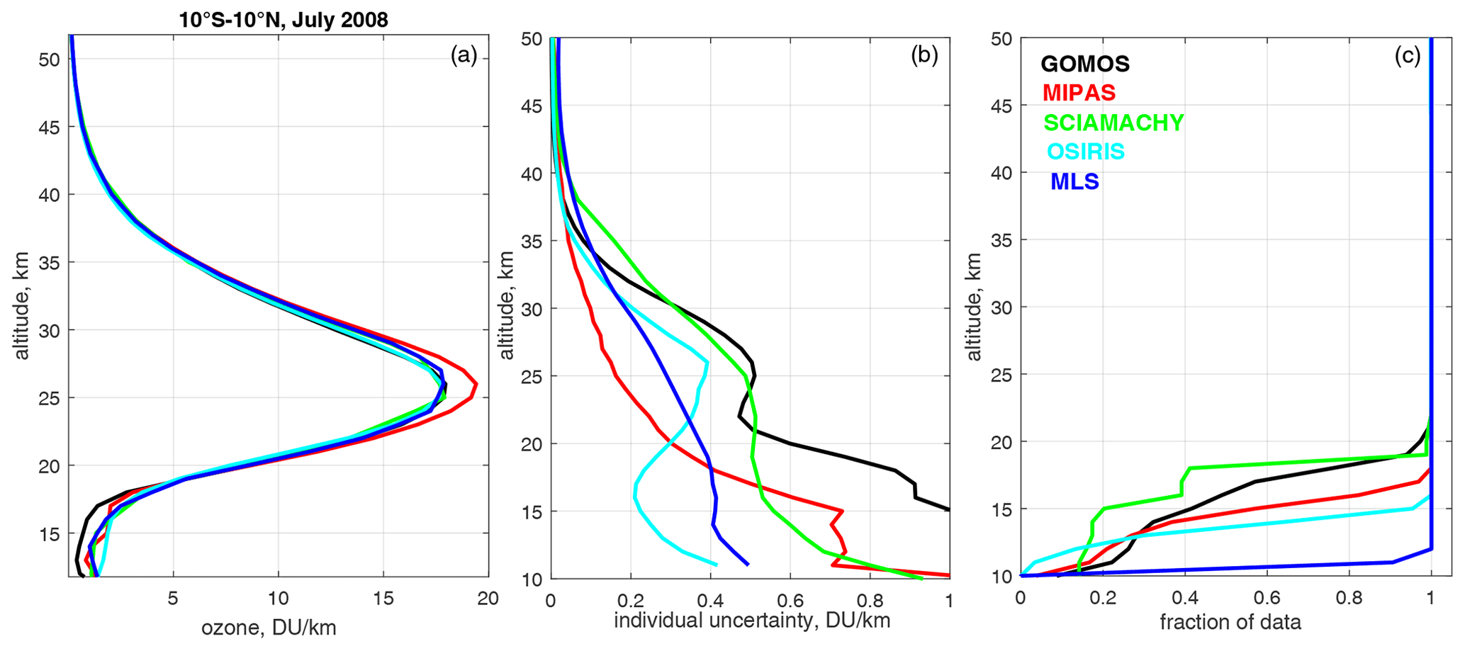
Figure 1 (a) Mean ozone profiles at 10^∘ S–10^∘ N in July 2008. (b) Uncertainty of individual ozone profiles. (c) Fraction of data (with respect to the data in the stratosphere).

For all limb instruments, we use the ozone profiles from the HARMonized dataset of Ozone profiles (HARMOZ) developed in the ESA Ozone_cci project (Sofieva et al., 2013; https://climate.esa.int/en/projects/ozone/data/, last access: 6 April 2022). HARMOZ consists of the original retrieved ozone profiles from each instrument, which are screened for invalid data by the instrument experts and are presented on a common vertical grid (the altitude-gridded profiles are used in our paper) and in a common netCDF4 format. The detailed information about the original datasets can be found in Sofieva et al. (2013).

2.3 SILAM chemistry transport model

The modeling tool used in the work is the System for Integrated modeLling of Atmospheric coMposition (SILAM; Sofiev et al., 2015; http://silam.fmi.fi/, last access: 6 April 2022). This is an offline chemistry transport model that has several unique features making it highly suitable for the current application. SILAM is a multi-scale model with seamless scaling from the global coverage down to regional scale with 1 km resolution (Korhonen et al., 2019; Kouznetsov et al., 2020; Sofiev et al., 2018; Xian et al., 2019). SILAM chemical and physical modules cover both the troposphere and the stratosphere (Hänninen et al., 2020; Kouznetsov and Sofiev, 2012; Sofiev, 2002; Sofiev et al., 2020).

SILAM is an extensively evaluated model, a member of the Copernicus Atmospheric Monitoring Service (CAMS) regional European ensemble (https://www.regional.atmosphere.copernicus.eu/, last access: 6 April 2022) and the Panda–MarcoPolo (an EU FP7 project) ensemble for Asia, both operational services with an established daily evaluation procedure (Brasseur et al., 2019; Kukkonen et al., 2012; Petersen et al., 2019; Xian et al., 2019). The model has also extended data assimilation capabilities (Sofiev, 2019; Vira et al., 2017; Vira and Sofiev, 2012, 2015).

In this work, we used the ozone profiles simulated with the new development of SILAM v5.7 with the horizontal resolution of $\mathrm{1}{}^{\circ }\times \mathrm{1}{}^{\circ }$ and the vertical grid as in the ERA-Interim dataset. Compared to v5.6, the new SILAM version has improved photolysis rates and advanced characterization of the cloud and aerosol effects, together with dry and wet deposition in which the scavenging has separate parameters for ice and water clouds. For meteorological parameters, we have moved from ERA-Interim to the new ERA5 dataset which has hourly time resolution. In addition, the newly implemented CBM05 (Carbon Bond Model from year 2005) chemistry module (https://camx-wp.azurewebsites.net/Files/CB05_Final_Report_120805.pdf, last access: 6 April 2022) provides better tropospheric ozone concentrations, especially in the tropics and in remote regions, compared with the previous CBM4 chemistry (Carbon Bond Model version 4; Gery et al., 1989, and updates).

For anthropogenic emissions, we use CAMS (Copernicus Atmosphere Monitoring Service) global emission database (v2.1) together with EDGAR4.3.2 emissions for aviation and partly self-made emissions for the most important CFC (chlorofluorocarbons ) compounds. In addition, SILAM takes into account biogenic emissions of isoprene and monoterpene (database based on the MEGAN (Model of Emissions of Gases and Aerosols from Nature) model), sea-salt emissions (including its small bromine fraction), dust emissions, and NO_x emissions from lightning. Emissions from fires are also included, using either IS4FIRES (see http://silam.fmi.fi/fires.html, last access: 6 April 2022) or other emission inventories.

For the majority of analyses presented in this paper, daily averaged ozone fields are used.

3 Feasibility studies on residual method to retrieve tropospheric ozone

3.1 Tropospheric ozone features observable by the residual method

About 90 % of ozone is in the stratosphere (the ozone layer). Figure 2 shows a typical ozone profile for the equatorial region (in units of DU km⁻¹) with indicated contributions from different layers. The challenges associated with the residual method are clearly seen in Fig. 2: the ozone in the UTLS has nearly the same abundance as the lower-tropospheric ozone, both much smaller than the stratospheric ozone column.

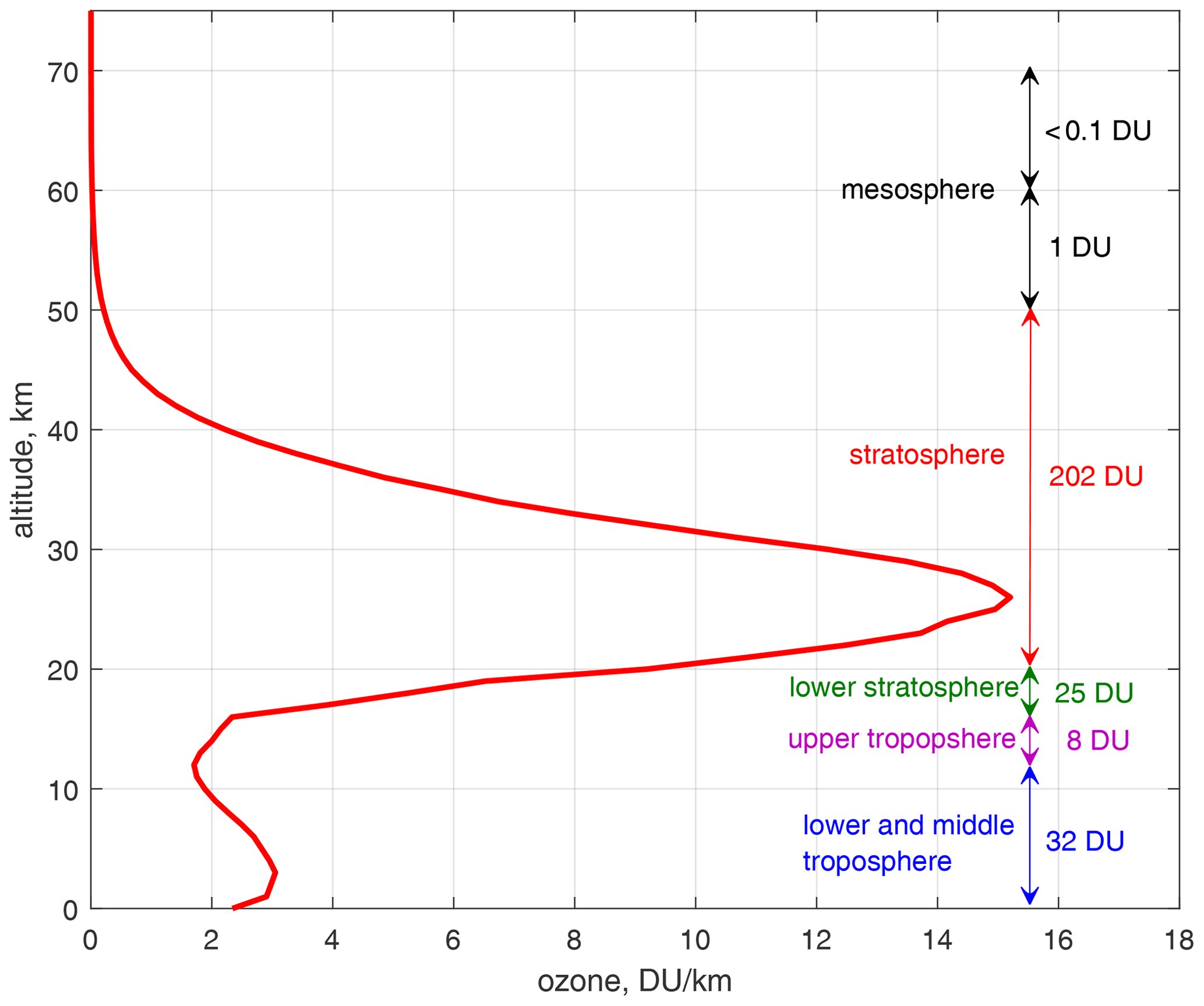
Figure 2 A schematic presentation of ozone profile (typical for the equatorial region), with indicated approximate contributions of different layers to the total ozone column.

The ozone enhancement in the troposphere at altitudes below 5 km is a result of complicated interplays of chemical production and loss mechanisms controlled by the abundance of the key chemical agents (NO_x and volatile organics), environmental conditions (solar radiation and temperature), and surface uptake by vegetation (e.g., Seinfeld and Pandis, 2006). Revealing the resulting patterns is therefore a challenging task, especially because these high-frequency spatial and temporal fluctuations have to be distinguished from fluctuations in the ozone layer and noise in the limb observations, which can be comparable with the tropospheric signal itself.

To facilitate the development of the residual method and find the best feasible spatiotemporal resolution for the dataset, we have performed feasibility analyses with the SILAM CTM. The model data are either used in their entirety or subsampled at the locations and times of satellite measurements.

Throughout this paper, the thermal tropopause definition is used to distinguish between the troposphere and the stratosphere (WMO, 1957). In some special cases at high latitudes, when this definition fails to find the tropopause, we use an ozone pause defined as the altitude where the ozone concentration gradient drops (looking from the stratosphere) down to 3.5 DU km⁻¹.

3.2 The effect of vertical extent

When considering the tropospheric ozone column, it is expected that the ground-level ozone enhancements will be clearly visible but smeared out and displaced due to advection. This feature is illustrated in Fig. 3, which compares the ground-level SILAM ozone data (Fig. 3, left panels) with the tropospheric ozone columns reaching from the ground either up to 3 km below the tropopause or up to the tropopause (Fig. 3, center and right panels, respectively) for 1 July 2008 (upper panels) and averaged over the whole month (bottom panels).

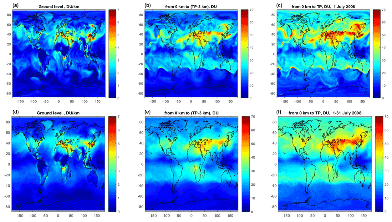
Figure 3 Simulations with SILAM for 1 July 2008 (a, b, c) and monthly mean for July 2008 (d, e, f). (a, d) Ground-level ozone, (b, e) truncated tropospheric ozone column (from ground to the altitude 3 km lower than the tropopause), and (c, f) the full tropospheric ozone column (from ground to the tropopause).

As seen from Fig. 3, the tropospheric ozone column (integrated from the surface to the tropopause and referred hereafter as full tropospheric ozone column, “full TrOC”; Fig. 3, right panels) has a large portion of ozone from the upper troposphere so that the tropospheric features (especially close to the ground level) are significantly blurred in the tropospheric column. If we consider the altitude range from the ground to 3 km below the thermal tropopause (referred to as “truncated TrOC”; Fig. 3, center panels), the influence of the upper troposphere is smaller but still significant.

In the monthly averaged fields (Fig. 3, bottom panels), the ground-level ozone enhancements are visible but smoothed. The choice of the upper limit of the tropospheric ozone integration (up to tropopause or below; compare central and right panels in Fig. 3) influences the overall level of the tropospheric ozone column (as expected) and also the contrast of the local enhancements. The higher contrast of the details visible from the truncated TrOC is advantageous for detecting the lower-tropospheric structures.

Since the quality of the limb-profile data (both accuracy and coverage) in the UTLS is limited, one can consider the possibility of estimating the upper-tropospheric ozone (for example, the layer of 3 km below the tropopause) and subtracting it from the full TrOC (analogy of ghost column correction in retrievals from nadir-looking instruments). To illustrate the effect, we simulated two approximate corrections of the upper-tropospheric ozone. In the first correction, the upper-tropospheric (UT, from 3 km below the tropopause up to the tropopause) monthly zonal mean ozone column was computed from the SILAM data for each latitude zone and subtracted from each data point of full TrOC for each day. In the second correction, the UT ozone column correction is done using the tropopause-related ozone climatology TpO3 (Sofieva et al., 2014). We found that even such very approximate upper-tropospheric ozone corrections give the monthly map of truncated TrOC nearly identical to the true one (Fig. S1, right panels, in the Supplement), with the difference to the true values mostly smaller than ±3 DU. However, we would like to note that the upper-tropospheric correction described above is a very approximate one (as any correction by climatological values) and can work properly only if the dominating ground sources do not change their strength and location. In our processing, we apply a more sophisticated upper-tropospheric correction; it will be described in detail in Sect. 4.

3.3 The effect of sampling and averaging kernel

The daily horizontal coverage by limb instruments is limited (see examples in Sect. 4.3). If the monthly mean stratospheric ozone column (SOC) is computed via simply averaging the data with such sampling, the resulting SOC has significant deviations from the SOC computed using the full ozone field because different pixels are covered by data from different days. The approach of averaging first the stratospheric ozone column and then subtracting it from the averaged total ozone column produces pronounced errors due to limited sampling by limb instruments (illustration can be found in Fig. S2). This implies that the monthly average of the tropospheric ozone column should be constructed from its daily values.

The tropospheric ozone column computed via averaging daily TrOC obtained by the residual method is quite close to the true distribution using the data with full coverage. This is illustrated in Fig. 4a and b. Figure 4c shows an analogous estimate of the tropospheric ozone, in which the total ozone column was computed with the OMI averaging kernels taken into account (the examples of OMI and TROPOMI averaging kernels are shown in Fig. S3). Since OMI and TROPOMI are sensitive to middle- and upper-tropospheric ozone (Fig. S3), the tropospheric ozone column derived by the residual method also misses a substantial fraction of the near-surface pattern. An interesting feature, which is associated with the influence of the averaging kernel, is that the enhancements over central Africa are shifted to the Atlantic Ocean. This is a combined effect of OMI low sensitivity near the ground and wind advection of both ozone and its precursors towards the west in the middle troposphere.

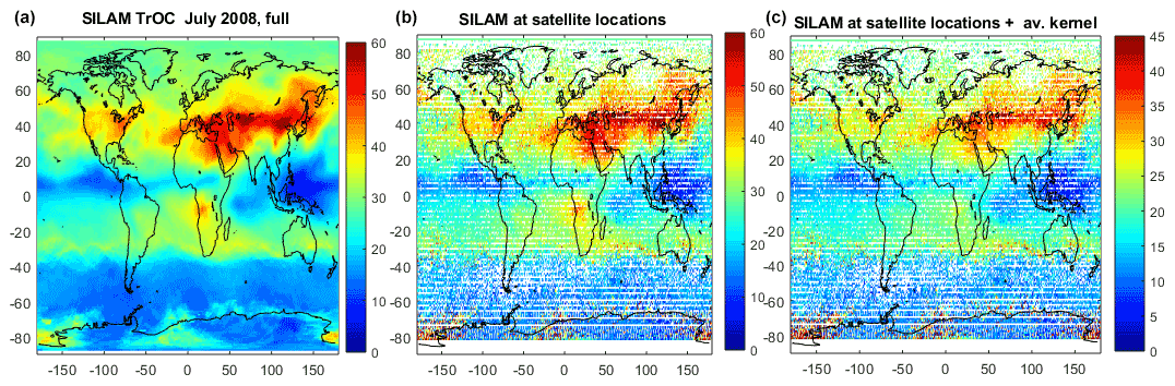
Figure 4 Estimates of full tropospheric ozone column (from the ground to the tropopause) using the application of the residual method to SILAM ozone profiles for the monthly average of July 2008. (a) TrOC is computed using the full SILAM ozone field, (b) SILAM data are subsampled at locations of nadir and limb satellite instruments, and (c) averaging kernel is taken into account in computing total ozone column at OMI locations. The sampling pattern corresponds to the combined dataset of GOMOS, MIPAS, SCIAMACHY, MLS, and OSIRIS measurements.

3.4 Conclusions from feasibility studies on the residual method

The following main conclusions can be drawn from the feasibility studies.

• In order to detect ground enhancements of tropospheric ozone, both the stratospheric and the UTLS contribution should be accurately removed from the nadir total ozone column data because the UTLS ozone contribution is comparable with the lower-tropospheric ozone abundances, and the stratospheric one largely exceeds it.

• The observed tropospheric ozone column enhancements are shifted from the near-surface production areas and blurred as a consequence of atmospheric motions and chemical transformations and limited sensitivity of nadir-looking satellite instruments in the lower troposphere.

• Due to large variability in the ozone field and limited sampling by satellite instruments, nadir and limb measurements should be collocated in time and space, if feasible.

• Upper-tropospheric ozone column correction using the data from an external source is an attractive approach which allows for the removal of the UT contribution from the full tropospheric ozone column without introducing large uncertainty into the truncated tropospheric ozone column.

Based on these studies, we have developed a method of estimating the tropospheric ozone column using the combination of limb and nadir measurements. The specific feature of our method is using the CTM-simulated ozone field in creating a high-spatial-resolution ozone field in the stratosphere and the UTLS.

In the next section we present the detailed description of the retrieval algorithms.

4 Tropospheric ozone column by the residual method

4.1 Methodology in general

We follow the general idea of the residual method, which consists of (1) creating a clear-sky total ozone column from nadir instruments, (2) creating a high-horizontal-resolution stratospheric ozone column by combining ozone profiles from several limb instruments, and (3) evaluating the tropospheric ozone column as the difference between the total and the stratospheric columns. The computations are done at the daily level with $\mathrm{1}{}^{\circ }\times \mathrm{1}{}^{\circ }$ spatial resolution; the daily tropospheric ozone columns are subsequently combined into the monthly mean column.

4.2 Gridded datasets from nadir instruments

To create the daily gridded total ozone column in $\mathrm{1}{}^{\circ }\times \mathrm{1}{}^{\circ }$ latitude–longitude bins (which are often referred to as Level 3), we used the clear-sky Level 2 data, with cloud fraction less than 0.2.

Since the OMI row anomaly (e.g., Schenkeveld et al., 2017) is not fully characterized by the processing flags, an additional adaptive data filtering was applied. First, we removed flagged pixels and one additional row from each side of the flagged region. The presence of a row anomaly was also checked by evaluating the ozone difference in neighboring rows. Along the swath direction, the anomaly is visible as a sudden drop and rise in the retrieved ozone column. The procedure was checking a difference in neighboring pixels; if a drop and a rise larger than 100 DU are detected, all pixels between these two points were removed. Finally, only the data with relative uncertainty less than 4 % were used for creating the daily gridded data.

In each latitude–longitude bin, the mean of total ozone column data is evaluated. The uncertainty of the total ozone column is computed as

$$\begin{array}{}\text{(1)}& {\mathit{\sigma }}^{\mathrm{2}}={\displaystyle \frac{\mathrm{1}}{N}}\sum _i{\mathit{\sigma }}_i^{\mathrm{2}}+{\displaystyle \frac{\mathrm{1}}{N}}\text{var}\left({\mathit{\rho }}_i\right),\end{array}$$

where σ_i are uncertainties reported by the retrieval algorithm, and var(ρ_i) is the variance of N individual ozone values in the bin. The typical daily gridded clear-sky total ozone column and the corresponding random uncertainties by Eq. (1) are shown in Fig. 5.

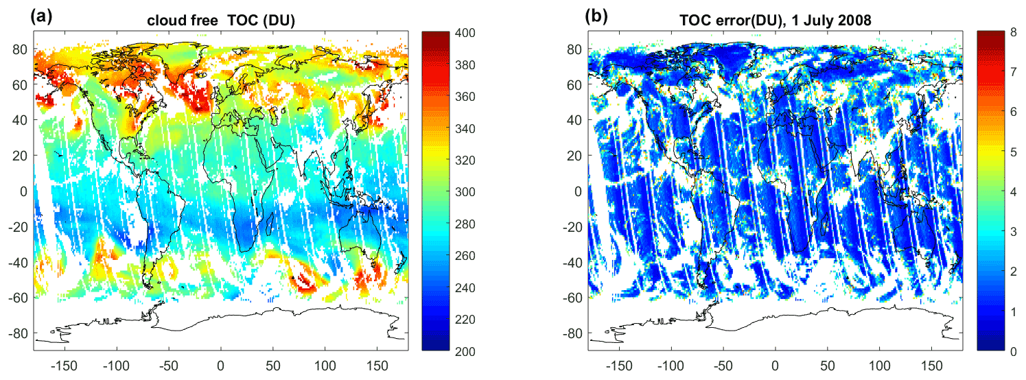
Figure 5 OMI Level 3 total ozone column data (a) and random uncertainty (b) for 1 July 2008.

The daily average gridded TROPOMI total ozone column data are computed in a similar way with the same spatial resolution of $\mathrm{1}{}^{\circ }\times \mathrm{1}{}^{\circ }$.

4.3 Homogenized and interpolated dataset of ozone profiles

In our approach, we first create the $\mathrm{1}{}^{\circ }\times \mathrm{1}{}^{\circ }$ gridded and interpolated dataset of ozone profiles, and then we computed stratospheric column via the integration of ozone profiles. We selected such an approach because the limb instruments have limited accuracy and highly non-uniform coverage in the UTLS, while the accurate knowledge of the UTLS profiles is essential for the application of the residual method (see details below).

In our algorithm, the creation of a homogenized interpolated dataset of ozone profiles consists of three main steps:

1. homogenization of ozone profile data from the limb satellite measurements;

2. interpolation of the limb profiles from each day to $\mathrm{1}{}^{\circ }\times \mathrm{1}{}^{\circ }$ horizontal grid;

3. a smooth transition to the adjusted model data below the tropopause.

Below we present the detailed description of the processing.

4.3.1 Homogenization of ozone profile data from the limb instruments

For horizontal interpolation, the data from different satellite measurements need to be compatible. As the first step of such data homogenization, biases between datasets are removed.

We use MLS as a reference dataset. For all other instruments, the biases with respect to MLS are evaluated for each month and for each latitude (with 1^∘ increments) using 10^∘ overlapping zones and corrected via adding latitude-dependent offset. This procedure removes the biases between the limb datasets, as illustrated in Fig. 6. After the bias correction, the data from different instruments can be used together. An example of bias-corrected data is shown also in Fig. 7a.

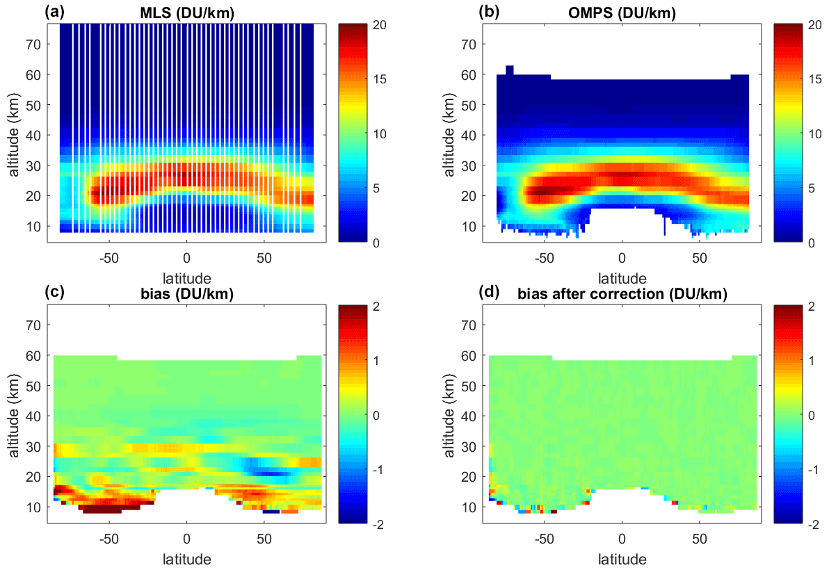
Figure 6 Illustration of the bias correction for September 2018. (a, b) MLS and OMPS profiles averaged over latitude zones and over the month. (c, d) Estimated OMPS biases before (c) and after (d) bias correction.

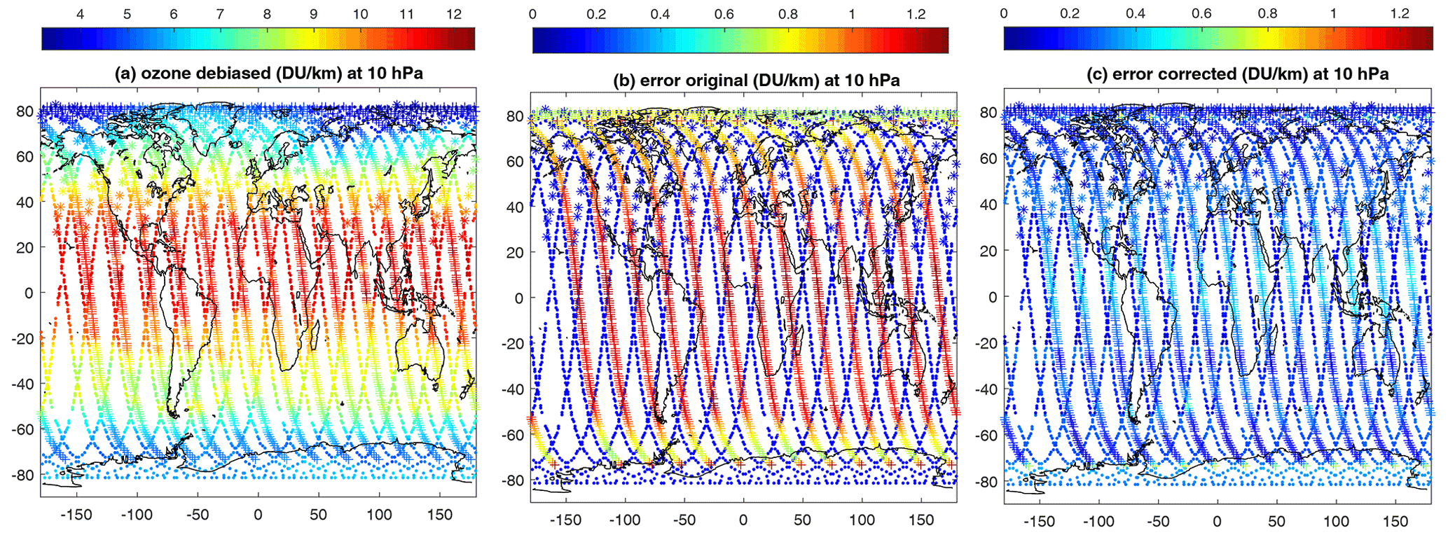
Figure 7 Debiased ozone at 10 hPa for 1 September 2018 (a), corresponding original uncertainties (b), and corrected uncertainties (c). MLS data are indicated by dots, OSIRIS by stars, and OMPS by plusses.

The optimal implementation of the horizontal interpolation method (see Sect. 4.3.2 for details) requires that the error estimates from different instruments agree and realistically describe the variations caused by random data uncertainties. However, this is not the case for the considered limb instruments: while biases between the instruments are rather small (within 10%), the estimated uncertainties can differ by an order of magnitude. This is illustrated in Fig. 7, which shows ozone and the reported uncertainties at 10 hPa for MLS, OSIRIS, and OMPS-LP (processed by the University of Saskatchewan v1.1.0). Uncertainty estimates of OMPS data processed by the University of Bremen have smaller differences with respect to MLS, but they still can differ by a factor of 2–3. The difference in error estimates depends on latitude, altitude, and season.

Therefore, we applied a simple approach that provides random uncertainties that are consistent with the variability field. For each instrument and each month, we evaluated sample variance s² in 10^∘ latitude zones from experimental data and the SILAM-adjusted field, which is subsampled at measurement locations. (The adjustment of SILAM data to MLS measurements is described in Sect. S2 in the Supplement.) This sample variance s² provides the estimates of natural variability ${\mathit{\sigma }}_{\mathrm{nat}}^{\mathrm{2}}$. Then a posteriori (ex post in von Clarmann et al., 2020, terminology) uncertainties can be estimated as ${\mathit{\sigma }}_{\mathrm{ex}\text{-}\mathrm{post}}^{\mathrm{2}}=s^{\mathrm{2}}-{\mathit{\sigma }}_{\mathrm{nat}}^{\mathrm{2}}$. We computed latitude- and altitude-dependent offset $\mathrm{\Delta }={\mathit{\sigma }}_{\mathrm{ex}\text{-}\mathrm{post}}-{\mathit{\sigma }}_{\mathrm{ex}\text{-}\mathrm{ante}}$ (σ_ex-ante is the mean error estimate provided with profiles in the same 10^∘ latitude zones over the month) and applied it to each profile. As shown in Fig. 7c, this simple correction of the uncertainty estimates makes them comparable. By construction, they are also compatible with the observed ozone variability.

4.3.2 Interpolation of the limb profiles

After homogenization, the limb data are interpolated to form a high-spatial-resolution dataset. For our application, the most attractive approach is a kriging-type interpolation, in which both data uncertainty and the structure of the data variability are taken into account. In this approach, the value at the point r is taken as a weighted mean of data in the neighborhood:

$$\begin{array}{}\text{(2)}& x\left(\mathit{r}\right)=\sum _i{w}_{i}x\left({\mathit{r}}_i\right),\end{array}$$

with the weights w_i inversely proportional to the total uncertainties:

$$\begin{array}{}\text{(3)}& {\mathit{\sigma }}_{\mathrm{tot},i}^{\mathrm{2}}={\mathit{\sigma }}_{\mathrm{noise},i}^{\mathrm{2}}+D\left({\mathit{r}}_i-\mathit{r}\right),\end{array}$$

where ${\mathit{\sigma }}_{\mathrm{noise}}^{\mathrm{2}}$ is the estimate of the noise in the data, and D(r_i−r) is the uncertainty due to the spatial mismatch, which is usually estimated via the structure function. The structure functions are widely used in studies of small-scale natural variability, and they can be used also for validation of random data uncertainties (Sofieva et al., 2021, and references therein). The evaluation of the structure functions is discussed also in Sect. S3. In our interpolation method, D(r_i−r) is taken from the adjusted SILAM field for each day. The weighted mean is assessed using the $\mathrm{10}{}^{\circ }\times \mathrm{20}{}^{\circ }$ latitude–longitude area around each point.

We have tested our interpolation scheme on the noise-free and the noisy simulated data with SILAM and found that the kriging-type interpolation described above is superior to the triangulation-type interpolation (for example, natural neighbor interpolation; Sibson et al., 1981): the interpolation error is smaller, and fine structures are better resolved. For noisy simulated data, the interpolation error is the smallest if the uncertainty estimates in Eq. (3) are realistic, as expected.

The interpolation of ozone profiles is performed at each pressure level separately. An example of the interpolated field is shown in Fig. 8.

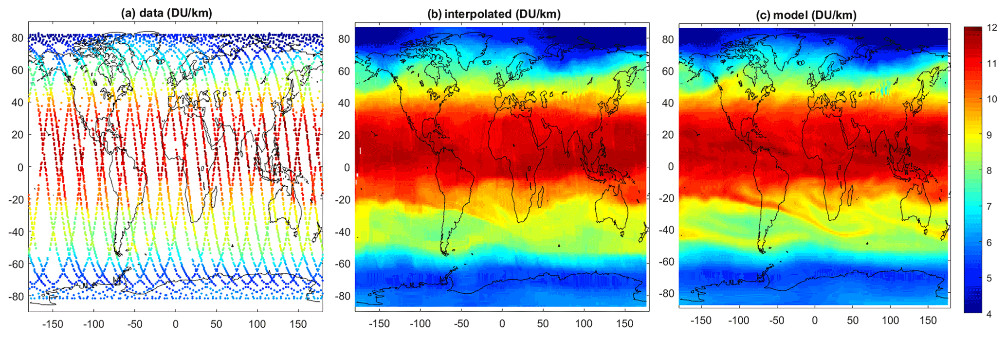
Figure 8 (a) Ozone at limb satellite measurements at 10 hPa on 1 September 2018. (b) Interpolated ozone at 10 hPa. (c) The corresponding adjusted SILAM ozone field at the same pressure level.

The uncertainties of the interpolated field are estimated as follows. The uncertainty after the kriging is estimated as the minimal value of σ_tot (Eq. 3) in the bin used for weighted mean. In addition, we estimated the interpolation uncertainty using the SILAM data: we applied the same interpolation on SILAM ozone subsampled at measurement locations and evaluated the error as the absolute difference of true and interpolated data. The final uncertainty is the root mean square of error propagation and model-assessed interpolation errors. The uncertainty estimation of the interpolated ozone field is illustrated in Sect. S4.

4.3.3 Extension into the troposphere

Since satellite data have limited accuracy and non-homogeneous and rather sparse coverage below the tropopause, we extended the satellite-based ozone profiles to lower altitudes by using the smooth transition to the adjusted SILAM profiles. The linear transition is performed in such a way that above 200 hPa the profile follows fully the experimental data and below 400 hPa fully the model data. The illustration of the transition to the model data at lower altitudes is shown in Fig. 9 for tropical and polar atmospheres.

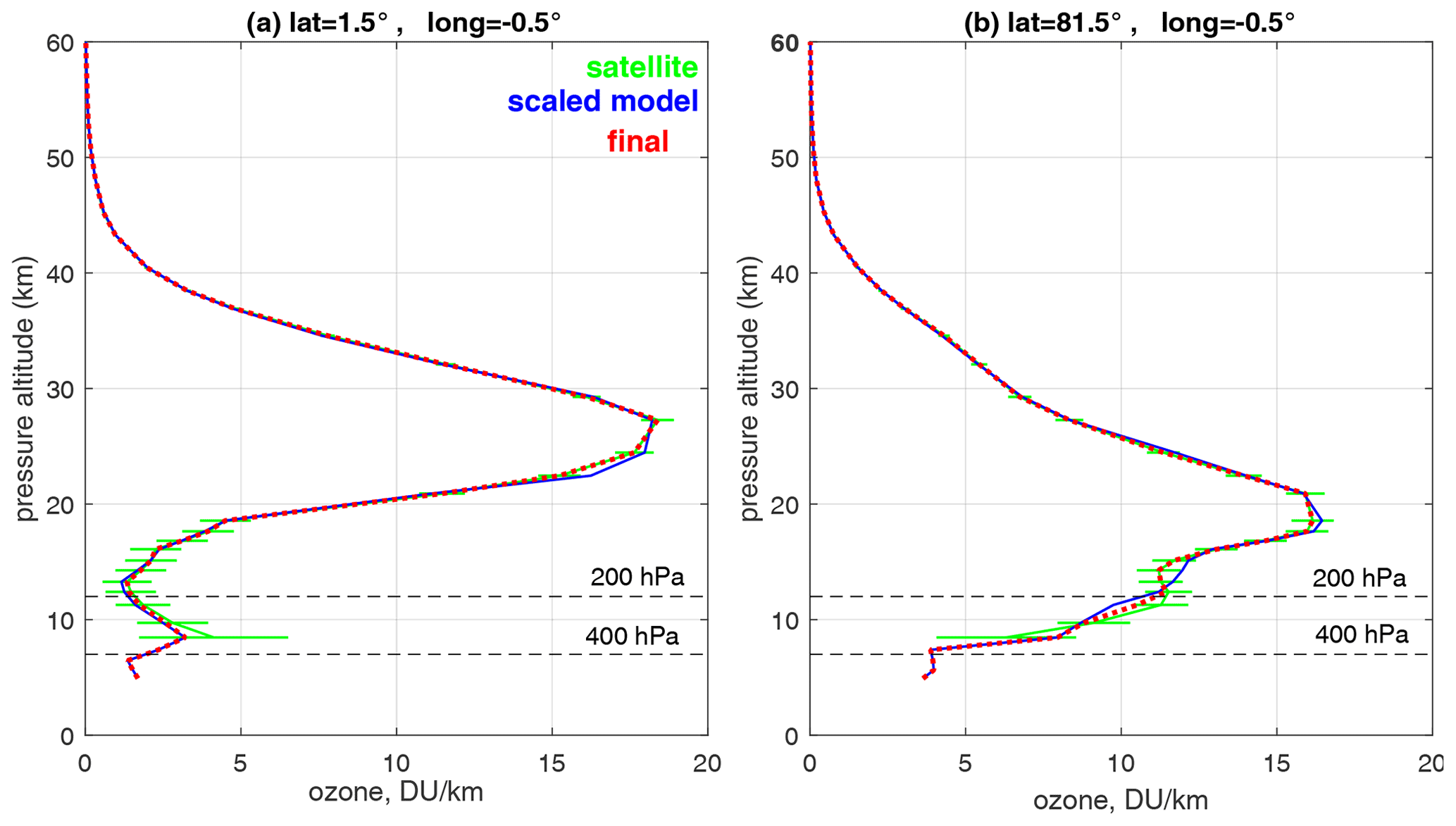
Figure 9 Illustration of transition to model-adjusted profiles at lower altitudes for tropical (a) and polar (b) regions. The vertical coordinate is pressure altitude $z=\mathrm{16}{\log }_{\mathrm{10}}(P_{\mathrm{0}}/P)$, where P₀=1013 hPa is the standard pressure, and P is pressure (in hPa).

Below in Sect. 5, we show that the resulting ozone profiles are in a good agreement with ozonesonde data.

4.4 Stratospheric ozone column dataset

Computing the stratospheric ozone column from the high-resolution profiles is rather straightforward. The integration can be done from the tropopause upwards (we use 55 km as the upper integration limit), or from a certain altitude level. Relatively high vertical resolution of limb instruments (2–4 km) and good accuracy (Table 1) allow accurate determination of the stratospheric ozone column. Limb ozone profiles were interpolated to 100 m altitude grid and integrated by the trapezoidal method. The uncertainties are estimated using the error propagation. The examples of stratospheric ozone columns from the tropopause and from 3 km below the tropopause and corresponding uncertainties are shown in Fig. 10. The estimated uncertainty of the derived stratospheric ozone column is mostly 5–8 DU (< 2 %).

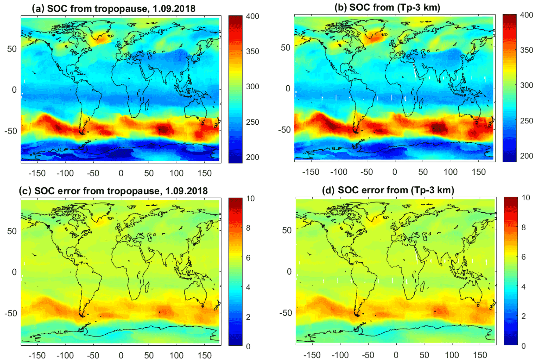
Figure 10 Stratospheric ozone column (DU) from the tropopause (a) and from 3 km below the tropopause (b) computed from $\mathrm{1}{}^{\circ }\times \mathrm{1}{}^{\circ }$ merged (homogenized and interpolated) limb ozone profiles. The corresponding uncertainties are shown in panels (c) and (d).

4.5 Tropospheric ozone column

Once the high-resolution stratospheric ozone column dataset is created, the application of the residual method is straightforward: the stratospheric columns are subtracted from the clear-sky measurements by the nadir sensors for each day. The daily values can be averaged to monthly mean values subsequently. Our tropospheric ozone column dataset is from ground to 3 km below the tropopause (truncated tropospheric ozone column). It corresponds to the local time of OMI and TROPOMI measurements.

Before the application of the residual method, the compatibility of limb and nadir data should be checked. For this, we compared OMI and TROPOMI measurements in cloudy conditions (the ghost column is removed) with the integrated ozone profiles from the cloud-top height. For this comparison, we selected cloudy pixels with cloud fraction >0.8, cloud-top pressure less than 350 hPa, and the corresponding limb profiles from the adjusted SILAM field. We found that over Indonesia and the western Pacific where high clouds are observed, the mean difference between nadir and limb instruments is very small, ∼2 DU, for both OMI and TROPOMI. The illustrations of this comparison can be found in Sect. S5. This correction estimate of 2 DU can be further tuned in the future when extensive validation of tropospheric ozone column data will be performed.

Although the compatibility of nadir and limb instruments in the tropics is good, there are possible data mismatches that lead to negative tropospheric ozone values at some pixels, which can be due to interpolation errors or the adjustments in the UTLS. Therefore, before averaging into the monthly mean tropospheric ozone data, we ignored the daily TrOC values smaller than −5 DU (but we allow small negative values, which can be due to noise).

Uncertainties of daily tropospheric ozone values are estimated as

$$\begin{array}{}\text{(4)}& {\mathit{\sigma }}_{\mathrm{TrOC}}^{\mathrm{2}}={\mathit{\sigma }}_{\mathrm{TOC}}^{\mathrm{2}}+{\mathit{\sigma }}_{\mathrm{SOC}}^{\mathrm{2}}.\end{array}$$

The uncertainties of monthly average data are estimated similarly to uncertainties in the gridded data, i.e., by Eq. (1).

After the averaging, we performed the additional data quality control and removed unreliable data from the dataset. First, we added an offset of 2 DU to the dataset, which removes the mean bias between limb and nadir stratospheric columns. Then we filtered the data with uncertainties larger than 200 % or smaller than 2 %. In the polar regions, the retrieval of tropospheric ozone has additional challenges due to the presence and perturbations of the polar vortex and loosely defined tropopause height. To exclude unrealistically large values at latitudes greater than 65^∘, we filtered out those data which are either larger than 80 DU or larger than 60 DU and with the relative uncertainty less than 10 %.

The resulting tropospheric ozone distributions from OMI and TROPOMI for September 2018 are shown in Fig. 11 (left panels). These distributions are very similar, but TROPOMI TrOC is less “noisy”. Typical ozone enhancements for September are observed: over Africa associated with forest fires, as well as over China and over Mediterranean regions. Zoom-ins on China and USA are shown in Fig. 12 in which one can observe the enhancements associated with large cities (but they are blurred and displaced, as expected).

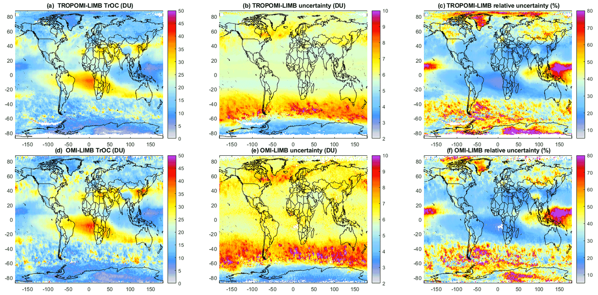
Figure 11 SUNLIT tropospheric ozone distributions (DU, color) for September 2018 from TROPOMI (a) and OMI (d). The stratospheric ozone column is estimated from 3 km below the tropopause. The corresponding estimated uncertainties are shown in absolute values (DU) in panels (b) and (e) and in relative values (%) in panels (c) and (f).

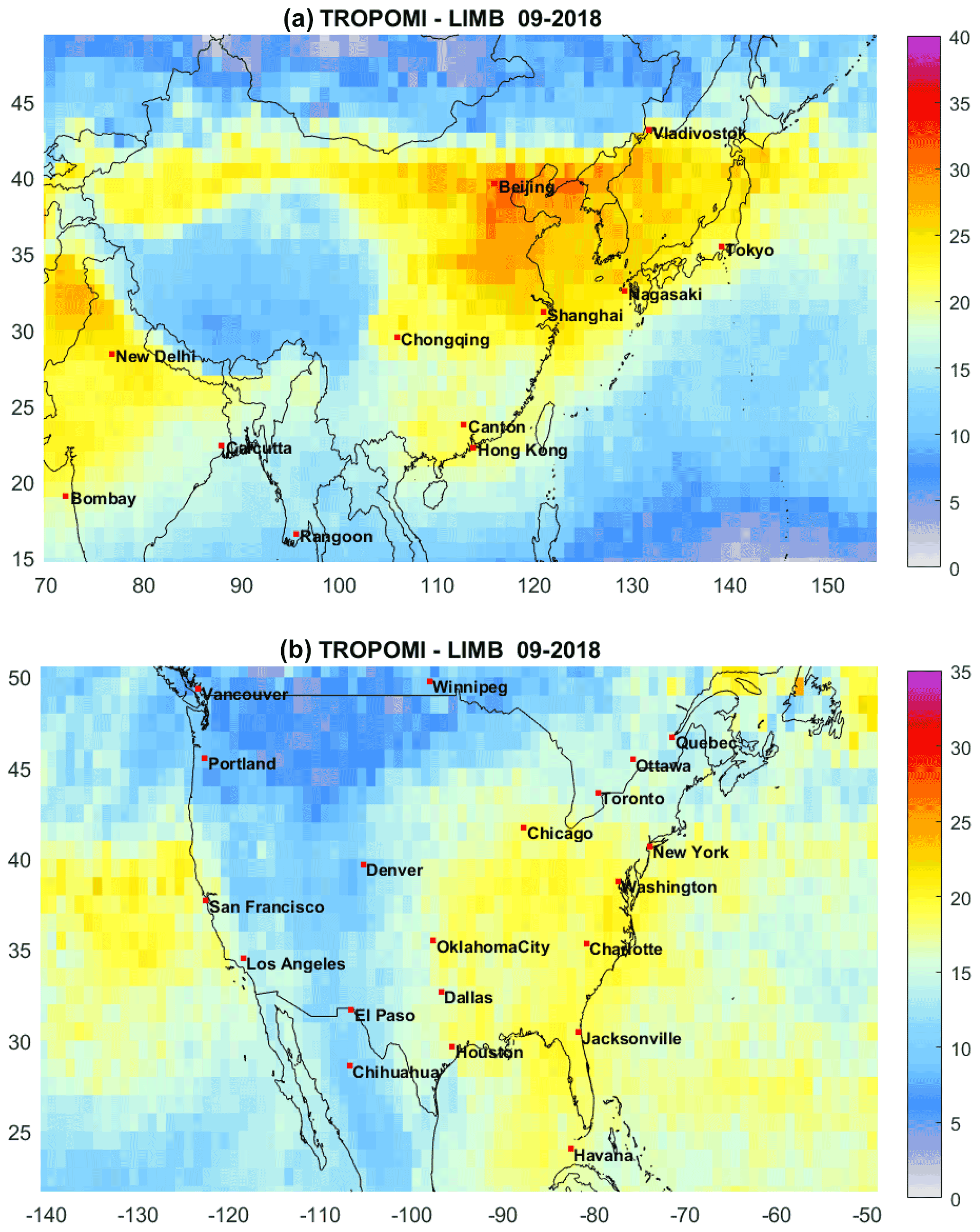
Figure 12 As in Fig. 11a but with zoom-in on China (a) and USA (b). Color indicates tropospheric ozone column in DU.

The estimated uncertainties for the September 2018 tropospheric ozone distributions from OMI and TROPOMI are shown in Fig. 11 in absolute values (DU) in the central panels and relative values (%) in the right panels. The uncertainties are slightly smaller for TROPOMI than for OMI. This is due to the more accurate TROPOMI total ozone column measurements and the better coverage: due to the better horizontal resolution, it is easier to find cloud-free data in $\mathrm{1}{}^{\circ }\times \mathrm{1}{}^{\circ }$ bins, which are used for evaluation of the tropospheric ozone column. In the majority of tropical locations, the estimated uncertainty of the tropospheric ozone column is 4–6 DU for TROPOMI and 5–7 DU for OMI. Over Indonesia, where the tropospheric ozone column has the smallest values, the relative uncertainty increases to 100 %. In the mid-latitudes of the Northern Hemisphere (summer season in August 2018), the estimated uncertainties are mostly within the range of 15 %–40 %. The largest uncertainty is close to the polar vortex boundary, as expected.

5 A limited validation and examples of the data

5.1 Comparisons of ozone profiles with ozone sondes

To assess the quality of the high-resolution SUNLIT ozone profiles, we compared them with the ozonesonde data. For this comparison, we used the collection of ozonesonde data from the BDBP database (Hassler et al., 2008) in 2004–2006. In these comparisons, ozonesonde data are smoothed down to 1 km vertical resolution, and they are collocated with SUNLIT data within a day and 1^∘ in latitude and longitude from the station location. The information about the selected ozonesonde data is collected in Table 2.

Table 2 Information about ozone sonde data used in comparisons.

Several examples – for polar, tropical, and mid-latitude stations, in winter and in summer – are shown in Fig. 13. As observed in this figure, ozonesonde and limb profiles are in very good agreement. The results of the statistics of differences (sonde minus satellite) for the selected stations – the median and 16th and 84th percentiles – are shown in Fig. 14. The biases are small in both the stratosphere and the troposphere; the inter-percentile range of differences is a few percent in the stratosphere and in the range of 10 %–50 % in the UTLS and the troposphere.

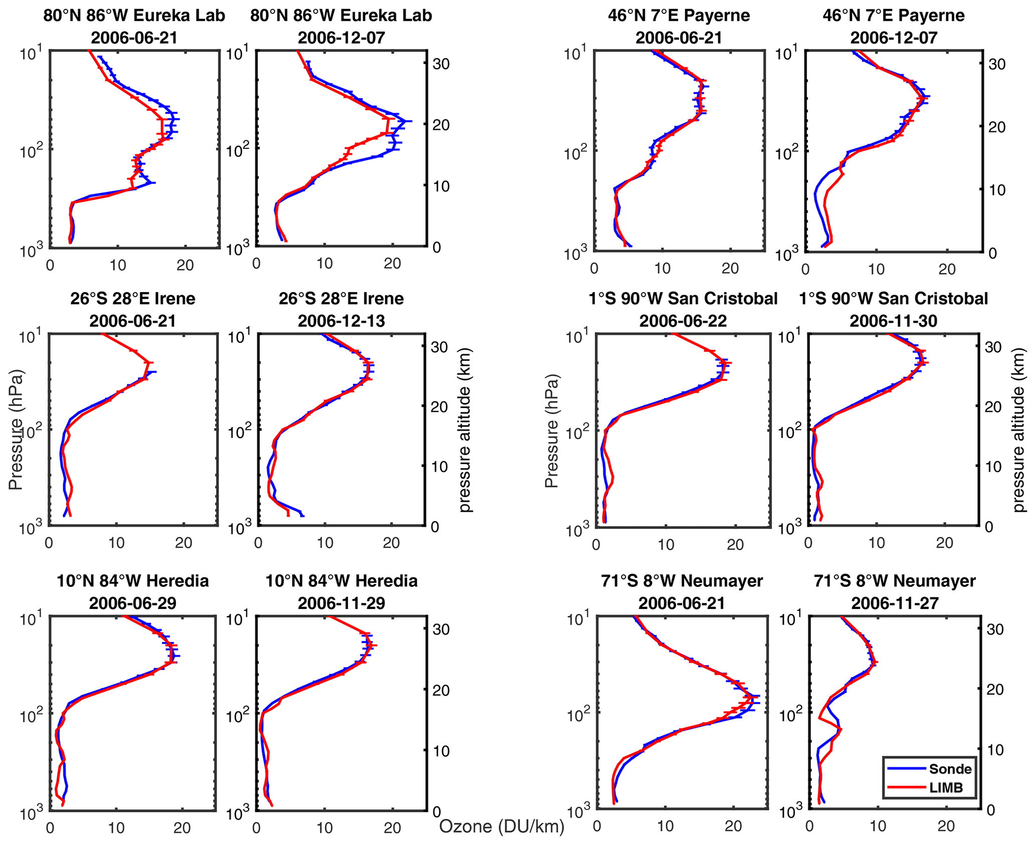
Figure 13 Several examples of ozonesonde data (blue lines with 1σ uncertainties) with the collocated interpolated limb profiles (red lines with 1σ uncertainties).

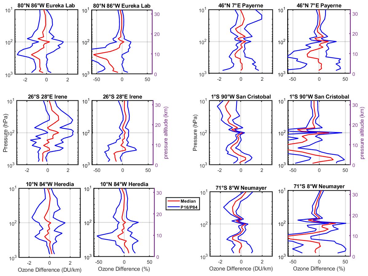
Figure 14 The statistical parameters of differences between ozonesonde and collocated interpolated limb profiles. The red lines show the median of absolute (left panels) and relative (right panels) differences, while blue lines show the 16th and 84th percentiles.

At two ozonesonde locations, i.e., stations Payerne and Paramaribo (SHADOZ – Southern Hemisphere ADditional OZonesondes; 5.75^∘ N, 55.2^∘ W), we plotted the time series of monthly mean truncated tropospheric ozone column (from ground to 3 km below the tropopause) from our processing (OMI-LIMB) and from integrated ozonesonde profiles (Fig. 15). The truncated tropospheric ozone column was computed as is (green lines) from ozonesonde profiles and with the application of the approximate OMI averaging kernel (as in Fig. S3) and averaged over a month. The uncertainties of monthly mean ozonesonde TrOC are computed as the standard error of the mean. Since we provide tropospheric ozone columns as monthly mean data, the ozonesonde TrOC values are also presented at monthly temporal resolution. However, we can expect only a broad agreement from such a comparison, as the temporal sampling of satellite and ozonesondes is different. As observed in Fig. 15, SUNLIT and ozonesonde time series of tropospheric ozone are in rather good agreement: the variations are similar. The seasonal cycles (shown in left panels of Fig. 15) are very similar in SUNLIT and ozonesonde tropospheric ozone column data.

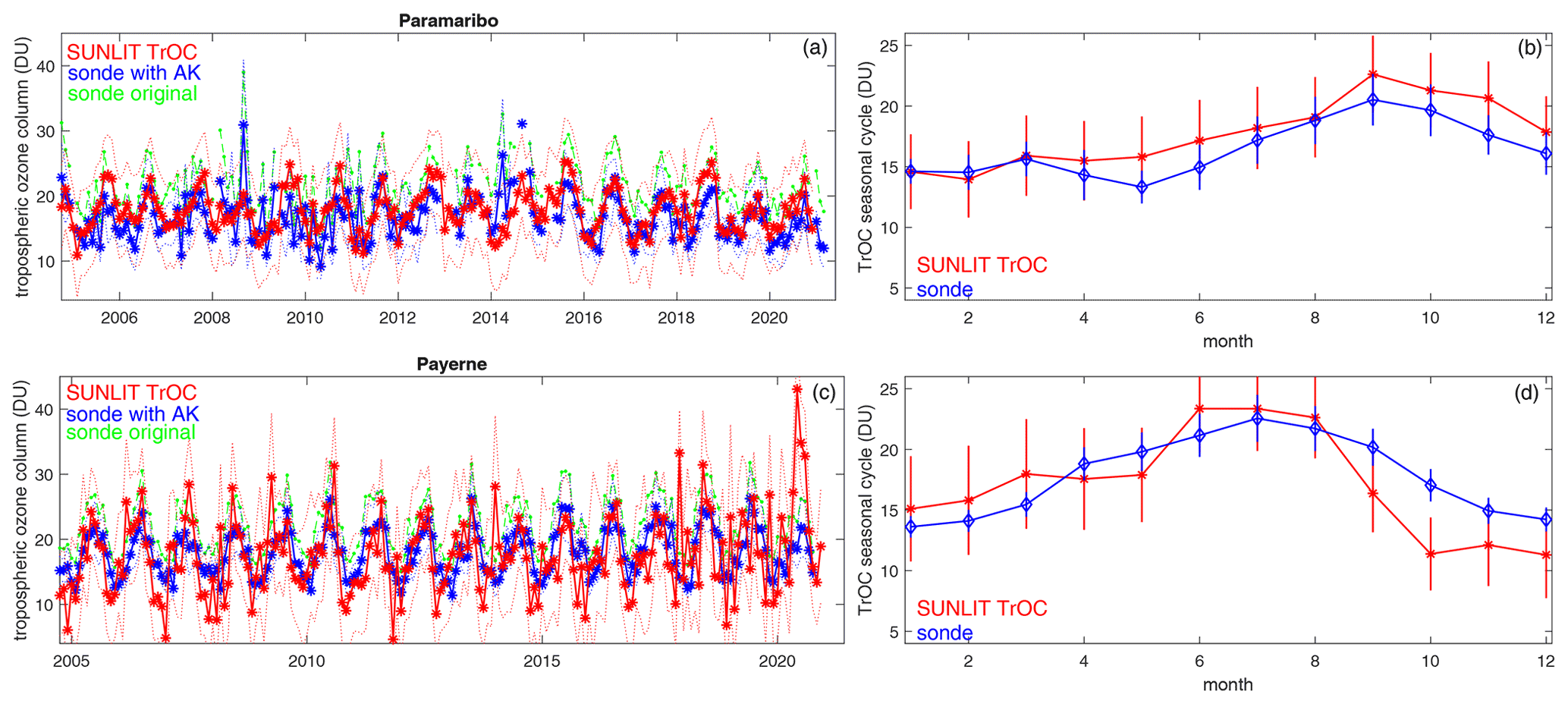
Figure 15 (a, c) Monthly mean tropospheric ozone column from ground to 3 km below tropopause altitude from OMI-LIMB (red line), integrated ozonesonde profiles (dashed green line), and integrated ozonesonde with approximate OMI averaging kernel applied (blue line, see text for details). Uncertainties for OMI-LIMB and ozonesonde TrOC with averaging kernel are indicated by dotted lines in panels (a) and (c). (b, d) Seasonal cycle with 2σ uncertainties for SUNLIT TrOC (OMI-LIMB) and ozonesonde TrOC.

In future analyses, it would be interesting to look at the similar behavior at the level of daily collocated satellite and ozonesonde data. Such an analysis would be also useful for assessing a possibility of providing a satellite-based tropospheric ozone column at a finer temporal resolution.

5.2 Comparison with OMI-MLS

For comparison with the NASA OMI-MLS tropospheric ozone column (obtained from https://acd-ext.gsfc.nasa.gov/Data_services/cloud_slice/new_data.html, last access: 6 April 2022), we computed the stratospheric ozone column from the tropopause, as is done in the OMI-MLS dataset. Examples of tropospheric ozone column for July 2008 are shown in Fig. 16. The SUNLIT tropospheric ozone distributions are provided also at high latitudes, while the OMI-MLS tropospheric ozone column is available from 60^∘ S to 60^∘ N. The overall ozone patterns are qualitatively very similar in both datasets. In particular, the enhanced values of tropospheric ozone are very close for SUNLIT and OMI-MLS datasets, while the low TrOC in the tropics over Indonesia is ∼5 DU smaller in the SUNLIT dataset than in OMI-MLS. Note that the main SUNLIT TrOC dataset, which we discussed in Sect. 4.5, spans over the altitude range from the ground to the 3 km below the tropopause. However, the availability of gridded interpolated ozone profiles from limb sensors allows the tropospheric ozone column with any upper limit to be estimated, as is done for the comparison with the OMI-MLS data.

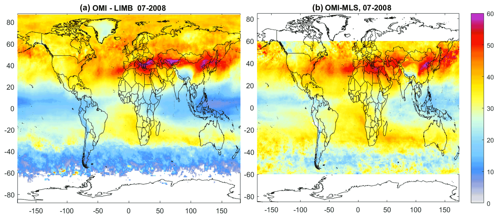
Figure 16 (a) SUNLIT tropospheric ozone column for July 2008 (OMI minus limb SOC); (b) NASA OMI-MLS tropospheric ozone column.

5.3 Comparison with CCD ozone

The convective cloud differential method (CCD) allows for retrievals of the tropospheric ozone column in the tropical region at latitudes of 20^∘ S–20^∘ N. The CCD tropospheric ozone dataset has been developed in the ozone CCI project; it represents the ozone column in the altitude range from ground to 10 km (Heue et al., 2016; https://climate.esa.int/en/projects/ozone/data/, last access: 6 April 2022). For comparison with the CCD tropospheric ozone column, we integrated the limb ozone profiles from 10 to 55 km and subtracted it from clear-sky total ozone column. The comparison of tropospheric ozone columns from the CCD method and from our computations are presented in Fig. 17.

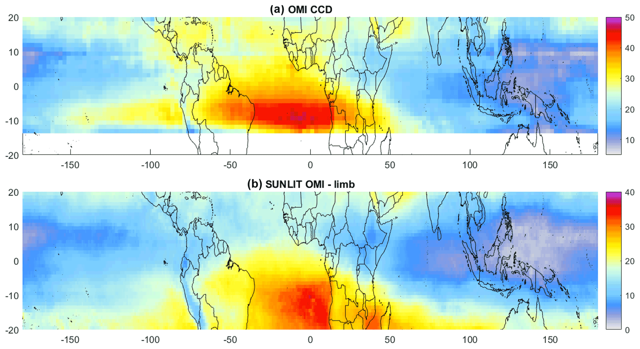
Figure 17 Tropospheric ozone column in DU (color) for September 2008 from (a) OMI CCD and (b) SUNLIT data (SOC is integrated from 10 km).

The morphology of the ozone distribution in the tropics in September 2008 is similar in the OMI-CCD dataset and in our tropospheric ozone column taken from the ground up to 10 km. However, the OMI-CCD TrOC values are ∼ 5–7 DU higher than in our analysis (note different color scales in the Fig. 17 panels). Heue et al. (2016) noticed a slightly larger (∼1.7 DU) tropospheric ozone from the CCD method than in the collocated ozonesonde values. Other differences can be due to using several nadir sensor data in the CCD dataset (OMI and GOME-2 (Global Ozone Monitoring Experiment-2) data are debiased to the SCIAMACHY dataset), as well as other approximations used in the processing of the CCD dataset (Heue et al., 2016).

The examples presented in this section show that the developed ozone datasets are in good agreement with ozonesonde and other satellite data. In general, intercomparison of tropospheric ozone data from different satellites and ground-based data is a complicated task because datasets can have different vertical extents and spatial and temporal sampling. The ongoing activity of TOAR-II (Tropospheric Ozone Assessment Report, Phase II; https://igacproject.org/activities/TOAR/TOAR-II, last access: 6 April 2022) aims at comprehensive intercomparisons of tropospheric ozone data. Our tropospheric datasets participate in this activity.

6 Summary

In this paper, we have presented the results of our studies on the methods for retrievals of the tropospheric ozone column by the residual method, i.e., the combination of total ozone column from nadir instruments with the stratospheric ozone column from limb instruments. The main result of our studies, which are performed in the framework of the ESA SUNLIT project, is the tropospheric ozone column (from ground to 3 km below the tropopause) datasets obtained by combining the OMI and TROPOMI total ozone columns with ozone profiles from the limb satellite instruments. The data are the monthly-averaged distributions with the horizontal resolution of $\mathrm{1}{}^{\circ }\times \mathrm{1}{}^{\circ }$. The derived tropospheric ozone column corresponds to the local time of OMI and TROPOMI measurements (∼ 13:30).

Other datasets, which are created as an intermediate step in creating the tropospheric ozone column data, can be used in other applications. These datasets are daily gridded with $\mathrm{1}{}^{\circ }\times \mathrm{1}{}^{\circ }$ horizontal resolution and include (i) a homogenized and interpolated dataset of ozone profiles from limb instruments, (ii) a stratospheric ozone column from limb instruments, and (iii) clear-sky and total ozone columns from nadir instruments.

The methodological developments made in our work include the method for homogenization of data from various satellite instruments and the method for horizontal interpolation, which takes into account both data uncertainties and variability in the parameter of interest.

The developed ozone datasets are in good agreement with ozone sonde and other satellite data. The global distributions of tropospheric ozone show clearly the enhancements associated with the regions of enhanced ozone production in the troposphere. The SUNLIT tropospheric ozone column dataset can be used in different analyses, including evaluation of long-term changes in the tropospheric ozone. This will be the subject of our work in the future.