the Creative Commons Attribution 4.0 License.
the Creative Commons Attribution 4.0 License.
 | 30 May 2022
A new scanning scheme and flexible retrieval for mean winds and gusts from Doppler lidar measurements
Julian Steinheuer
Carola Detring
Frank Beyrich
Ulrich Löhnert
Petra Friederichs
Stephanie Fiedler
Doppler wind lidars (DWLs) have increasingly been used over the last decade to derive the mean wind in the atmospheric boundary layer. DWLs allow the determination of wind vector profiles with high vertical resolution and provide an alternative to classic meteorological tower observations. They also receive signals from altitudes higher than a tower and can be set up flexibly in any power-supplied location. In this work, we address the question of whether and how wind gusts can be derived from DWL observations. The characterization of wind gusts is one central goal of the Field Experiment on Sub-Mesoscale Spatio-Temporal Variability in Lindenberg (FESSTVaL). Obtaining wind gusts from a DWL is not trivial because a monostatic DWL provides only a radial velocity per line of sight, i.e., only one component of a three-dimensional vector, and measurements in at least three linearly independent directions are required to derive the wind vector. Performing them sequentially limits the achievable time resolution, while wind gusts are short-lived phenomena. This study compares different DWL configurations in terms of their potential to derive wind gusts. For this purpose, we develop a new wind retrieval method that is applicable to different scanning configurations and various time resolutions. We test eight configurations with StreamLine DWL systems from HALO Photonics and evaluate gust peaks and mean wind over 10 min at 90 m a.g.l. against a sonic anemometer at the meteorological tower in Falkenberg, Germany. The best-performing configuration for retrieving wind gusts proves to be a fast continuous scanning mode (CSM) that completes a full observation cycle within 3.4 s. During this time interval, about 11 radial Doppler velocities are measured, which are then used to retrieve single gusts. The fast CSM configuration was successfully operated over a 3-month period in summer 2020. The CSM paired with our new retrieval technique provides gust peaks that compare well to classic sonic anemometer measurements from the meteorological tower.
- Article
(5935 KB) - Full-text XML
- BibTeX
- EndNote


Extreme wind situations are responsible for many weather-related hazards. The most important weather parameter for the amount of associated damage is the peak wind gust (e.g., Pasztor et al., 2014; Jung et al., 2016; Schindler et al., 2016). This is generally considered in both the standard observational network and in the diagnostic of numerical weather forecasts at 10 m above ground level (World Meteorological Organization, 2018; Brasseur, 2001; Schreur and Geertsema, 2008; Sheridan, 2011). Information on wind gusts from higher altitudes is therefore less frequently available. However, vertically available information about wind gusts would help to better predict wind-related hazards and to identify vulnerable locations in this context, which is useful, for example, for the design of larger buildings or wind turbines.
The short-term nature of wind gusts makes them difficult to observe accurately. In addition, there are different definitions of wind gusts. According to the World Meteorological Organization (2018), a wind gust is a short-lived significant increase in wind speed that lasts at least 3 s. Wind gust peak, or briefly gust peak, refers to the maximum wind gust in a given time window, e.g., within 10 min. A measuring device must therefore resolve the wind speed with high temporal resolution. The most advanced instruments are sonic anemometers that measure wind at sampling frequencies of up to 100 Hz, whereas typical sampling rates for routine wind measurements at national meteorological services are 1–4 Hz. The advantage is that these are in situ measurements. However, the instruments must be attached to taller structures, so these can strongly influence the measurements, such as can be observed in the wake of wind turbines (González-Longatt et al., 2012). Long-term gust observations above 10 m are collected at meteorological tower sites equipped with sonic anemometers. The installation of a meteorological tower site is expensive and requires regular maintenance afterwards. Usually, this effort is carried out by research institutions and national meteorological services at only a few sites, e.g., at Hamburg, Karlsruhe, and Cabauw (Brümmer et al., 2012; Kohler et al., 2017; Bosveld et al., 2020). Accordingly, the spatial coverage with such observations is sparse. Moreover, the height of such towers is limited to about 300 m, and hence no long-term observations can be made above this height.
The use of Doppler wind lidars (DWLs) overcomes some of the limitations of meteorological towers, as they are remote sensing devices. These have become increasingly important in recent decades, in part because they have become less expensive (Emeis et al., 2007). Further, DWLs are portable instruments that can be set up with considerably less effort than a tower. They provide reliable vertical profiles of mean wind in the lower atmospheric boundary layer under most conditions (Päschke et al., 2015). However, it is unclear whether they are suitable for retrieving highly fluctuating gusts. A DWL measures Doppler velocities along different beam directions to determine the three-dimensional wind vector. Therefore, a DWL must observe a larger volume of air to infer the wind vector. As a result, unlike an in situ instrument, a DWL cannot provide a high-resolution time series of wind vectors at a specific point in space. Accordingly, small-scale wind variations may be noticeable only in certain regions of the sampled air volume, and not all determined Doppler velocities may be affected the same way. For the strongest gust peaks, we assume that they also occur over a larger area by realizing that the air parcels with increased velocities travel a longer distance in a given time interval. Thus, we assume that strong gusts influence the measured Doppler velocities to a sufficient extent over the whole sampling volume. However, a fast measurement configuration for the DWL is required to obtain gust peak estimates comparable to measurements by a sonic anemometer of wind peaks lasting 3 s.
Suomi et al. (2017) propose a method for determining wind gusts using WindCube V2 DWL measurements. The DWL they considered operated for 2 d in a Doppler beam swinging (DBS) mode that provides measurements of five beams per one configuration cycle in 3.8 s. Wind vectors are derived from each set of five measurements, and gust peaks are obtained from them. The approach includes a scaling method for the detected 3.8 s gusts to infer 3 s gusts. This way, the results agree well with 3 s gust peaks as measured by a nearby sonic anemometer on a meteorological tower. The considered observation period is very short, and it remains open whether another measurement configuration is also suitable.
Within the Field Experiment on Sub-Mesoscale Spatio-Temporal Variability in Lindenberg (FESSTVaL, Fig. 1a), different sub-mesoscale phenomena in the atmospheric boundary layer are investigated. These include various observations and high-resolution modeling. Both address phenomena such as the evolution of the diurnal boundary layer, taking into account its turbulent nature, and the evolution of wind gusts. For this purpose, multiple institutions gathered a variety of measuring devices in order to create a comprehensive observation network. A number of DWLs are involved, which were deployed at the boundary layer field site in Falkenberg next to a 99 m high meteorological tower. The tower is equipped with sonic anemometers, which routinely provide wind and turbulence information.
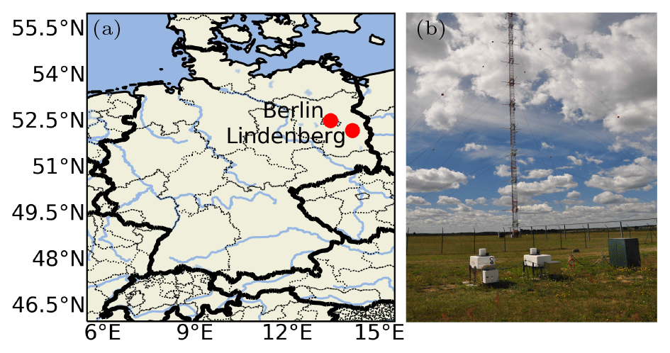
Figure 1Measurement site. (a) The MOL-RAO is situated in the northeastern part of Germany, approximately 65 km southeast of Berlin. (b) Two Doppler wind lidars in front of Falkenberg meteorological tower (27 July 2020, author's photo); Falkenberg is approximately 5 km south of Lindenberg.
In this study, we will focus on the deployed DWLs and their ability to retrieve wind gusts. Up to three colocated DWLs are used to test different measuring configurations in parallel. The available DWL devices, StreamLine from HALO Photonics, cannot achieve the DBS scanning configuration in 3.8 s, but they are very flexible when it comes to setting up other measurement configurations. The results are compared with measurements from the sonic anemometer at 90.3 m. When exploring different DWL scan configurations, it turns out that a fast continuous scanning mode (CSM) is capable of completing a single revolution of the scanning head within 3.4 s. This configuration is thus closest to the gust definition and is therefore tested over an extended period during the 3 summer months of 2020. For the calculation of the wind vectors, we develop a new retrieval scheme that can be used flexibly for different scanning configurations, for any number of observations, and for any desired time interval down to the duration of a single sampling cone. All results are derived from the new retrieval, which, in addition to calculating the gust peaks, is also used to determine the 10 min mean wind, since a practical configuration must also correctly capture the mean wind.
In Sect. 2, we first provide an overview of the wind measuring devices, from which the data were obtained during FESSTVaL. Here we also describe in more detail the different tested DWL configurations. Section 3 introduces the new retrieval with an integrated iterative noise filtering. Section 4 provides the results and is structured in three parts that report on the test campaign in 2019–2020, demonstrate the capabilities of the new retrieval scheme during the extratropical cyclone Sabine in February 2020, and give 3-month statistics on the DWL performance with the CSM in summer 2020. The paper is concluded in Sect. 5 with prospective plans for the evaluation of further FESSTVaL observations.
The measurements analyzed here are part of the FESSTVaL campaign. Originally, the FESSTVaL campaign was planned for 2020, but it had to be postponed to 2021 as a result of the Covid-19 pandemic, and its evaluation is not part of the presented work. Here, we will evaluate the 2019 test campaign and the reduced 2020 campaign, called FESST@MOL, in which fewer measurements were made than initially planned but with DWL observations involved. In the 2019 test campaign, different configurations were investigated with up to three DWLs. In 2020, one of these DWLs was in operation when extratropical cyclone Sabine passed in February and during the 3 summer months.
All instruments were operated at the boundary layer field site (in German: Grenzschichtmessfeld, GM) at Falkenberg (52∘10′ N, 14∘07′ E, 73 m above mean sea level). The GM Falkenberg is operated by the Meteorological Observatory Lindenberg – Richard Aßmann Observatory (MOL-RAO) and is located about 5 km south of the Lindenberg observatory site, which is approximately 65 km southeast of Berlin, Germany (Fig.1a). The measurement field is situated in flat terrain and surrounded by agricultural land. There is a 99 m high meteorological tower at the field site, where sonic anemometers regularly measure wind and turbulence. Further information is given in Sect. 2.1. The DWLs were deployed at about 70 m of distance from the meteorological tower (Fig.1b). Further information on the general measuring principle and the different configurations of the DWL is given in Sect. 2.2 and 2.3.
2.1 Sonic wind anemometer measurements
The meteorological tower at the GM Falkenberg site is equipped with two sonic anemometers at 50.3 and 90.3 m height. These ultrasonic wind anemometers are manufactured by Metek (factory version USA-1) and resolve the wind vector with a high temporal resolution of 20 Hz. Since the first usable DWL measurements are above 50.3 m, the measurement height of 90.3 m is taken as the reference for validation. To ensure data quality of the sonic anemometer measurements three main steps of operational data quality control are realized: filter nonphysical and constant values, detect spikes, and replace them by interpolating the neighboring points. Constant values can occur when the sonic anemometer is not working properly; for instance, when it is frozen for a short time and sends the last measured value until a new measurement is available. Unrealistic spikes are detected following Vickers and Mahrt (1997) and replaced by a linear interpolation of the neighboring values. Despiking is very rarely used, and strong gusts are not removed by the procedure because they are characterized by a persistent signal in successive measurements that are technically not spikes. The filtered and corrected time series are used to calculate the 10 min mean and the 3 s gust peak, which is derived from a moving average over 60 single measurements within each 10 min interval. Thus, the sonic anemometer gust peak represents a high-resolution reference for the DWL validation. The sonic anemometer at 90.3 m is located on a boom pointing towards the south from the tower. The distance to the tower construction is 4 m. Due to shadowing effects caused by the meteorological tower itself, measured values from wind directions of 0–50∘ are disturbed and must be discarded in a fair evaluation. These are winds from the north-northeast and thus not from a very frequently occurring direction in Falkenberg. For the comparisons of the sonic anemometer and the DWL measurements, only data from a wind direction sector between 50 and 360∘ are therefore analyzed.
2.2 Doppler wind lidar measurements
A DWL measures radial wind velocities along the beam direction of emitted light in the near-infrared part of the electromagnetic spectrum. The emitted laser pulses are backscattered by aerosols and received with a shifted frequency since the aerosols move with the wind. The range allocation of the backscattered signal follows from the traveling time. The Doppler shift in the light frequency enables the determination of the radial velocity, which is therefore referred to as the Doppler velocity. Figure 2 schematically illustrates the measurement principle. Each beam direction is determined by an elevation angle and an azimuth angle. The latter is counted clockwise from the north; i.e., 0∘ equals north and 90∘ equals east. The beam is divided into a series of range gates. Each received Doppler velocity is assigned to the center of a range gate. The corresponding height of the center of the range gates depends on its distance to the sensor and on the inclination of the beam. To allow comparison with the sonic anemometer, we linearly interpolate for each beam a virtual Doppler velocity at 90.3 m from the retrieved Doppler velocities at the two nearest range gates. The wind retrieval presented in the following section is then also applied to the interpolated Doppler velocities.
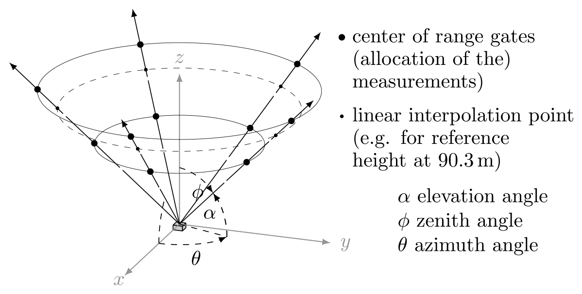
Figure 2The DWL observation principle is shown here with five beams per cycle. Each beam consists of several thousand laser pulses, and the backscattered signal is affiliated with a discrete series of range gates depending on the length of a single laser pulse and the traveling time. The resulting Doppler velocities are assigned to center-of-range gates. In order to obtain comparable results at intermediate heights, a linear interpolation between the two neighboring measurements along each beam is performed.
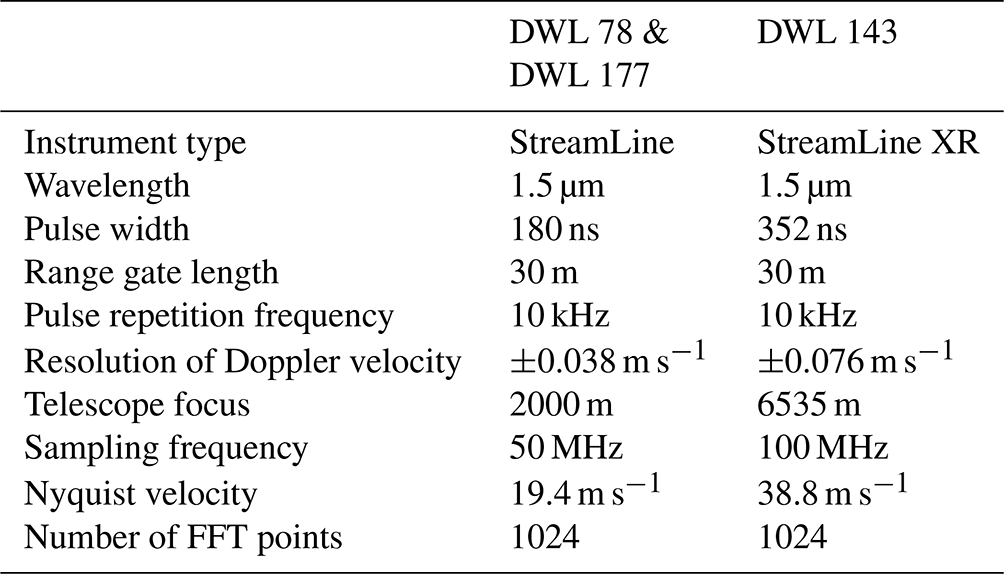
Three HALO Photonics DWLs have been part of the comparative test campaign – two of them (DWL 78 and DWL 177) are owned by the German Weather Service (in German: Deutscher Wetterdienst, DWD) and one is owned by the Technical University Berlin (DWL 143). A summary of their technical details is given in Table 1. The DWLs are flexible in setting up individual configurations. This involves the number of pulses per ray, the number of radial measurements required by the DWL to complete a single measurement cycle before repeating the configuration, and the elevation and azimuth of the beam direction. By using a smaller number of laser pulses per ray, a shorter duration to complete one measurement cycle is achievable. However, the accuracy of a single Doppler velocity may be reduced by using too few pulses. Typically, a DWL is operated in a step-stare mode; i.e., the DWL moves to an exact angular position, measures, and moves again, including acceleration and deceleration time. This time can be saved by setting up a continuous scanning mode wherein acceleration and deceleration are omitted and measurements are taken during motion of the DWL scan head. Here, the azimuth covers a specific window, and each Doppler velocity is assigned to an azimuth representative of that window.
Table 1Instrument parameters of the three HALO Photonics StreamLine DWL systems.
2.3 Doppler wind lidar configurations
We present eight different configurations that are tested for their suitability for retrieving gusts. Figure 3 illustrates the configurations with the corresponding panels as in the following itemized list.

Figure 3The different tested DWL configurations with corresponding averaged cycle time (in parentheses), the total number of averaged pulses per measured Doppler velocity (p), their elevation angle (α) and azimuth step angle (Δθ), and the number of beams per cycle (n; for the continuous modes this is an approximated value).
- a.
CSM1 (75 s) is conducted in continuous scanning mode, completing one DWL cycle in 75 s with a 35.3∘ elevation angle. One measurement is performed with 3.000 pulses, and each cycle consists of about 210 beams, giving a relatively high spatial coverage. Smalikho and Banakh (2017) propose measuring continuously to determine the turbulent kinetic energy (TKE). The rather flat elevation angle of 35.3∘ is based on considerations by Eberhard et al. (1989), as this enables a convenient calculation of TKE.
- b.
24Beam (120 s) is conducted in step-stare mode in 120 s with a 75∘ elevation angle. One measurement is performed with 30 000 pulses, and each cycle consists of 24 beams of exactly 15∘ azimuth steps to each other. This configuration is a popular mode for mean wind measurements with a relatively steep elevation angle to obtain observations from higher altitudes. At Lindenberg, for instance, there is another DWL that has been operated in this configuration for several years (Päschke et al., 2015). Similar to the CSM1, the 24Beam is not fast, but it is worth testing in terms of its widespread usage.
- c.
DBS (28 s) is conducted in Doppler beam swinging in 28 s with a 62∘ elevation angle. One measurement is made with 30 000 pulses, and each cycle consists of four beams pointing north, east, south, and west as well as one vertical beam. This configuration was proposed by Suomi et al. (2017) for measuring wind gusts but originally with 3.8 s per cycle for the system used in their study. However, our HALO Photonics StreamLine DWLs do not reach this temporal resolution but require 28 s to complete one cycle. Thus, although the study of Suomi et al. offers a promising way to retrieve wind gusts, it is not directly implementable here, and it is questionable whether we can achieve comparable results and hence validate their approach.
- d.
6Beam (35 s) is conducted in step-stare mode with six beams in 35 s with a 45∘ elevation angle. One measurement is made with 20 000 pulses, and each cycle consists of five symmetrically arranged beams having an azimuth angle difference of Δθ=72∘ with respect to each other, as well as one vertical beam. Sathe et al. (2015) propose using this configuration to measure turbulence with a DWL. Six different measurements allow the estimation of the Reynolds stress tensor since it consists of six independent entries. Their approach uses an optimal elevation angle of α=45∘ for the inclined beams.
- e.
3Beam1 (18 s) is conducted in step-stare mode with three beams in 18 s with a 35.3∘ elevation angle. One measurement is made with 10 000 pulses, and each cycle consists of three beams having an azimuth angle difference of Δθ=120∘ with respect to each other. A relatively short temporal resolution can be achieved by using only three beams for a DWL cycle and a relatively small number of pulses for a step-stare mode. Note that when using only three measurements, the calculation of the wind vector uncertainty is not possible and the result is prone to error, so a rather smaller elevation angle is chosen to measure the horizontal wind more directly.
- f.
3Beam2 (24 s) is conducted in step-stare mode with three beams in 24 s with a 35.3∘ elevation angle. One measurement is made with 30 000 pulses, and each cycle consists of three beams having an azimuth angle difference of Δθ=120∘ with respect to each other. Using only three beams but 30 000 pulses per beam gives this configuration a duration of 24 s. It can be seen that tripling the transmission pulse rate from 10 000 to 30 000 pulses per ray does not increase the total cycle time significantly; or, expressed differently, no time resolution close to a 3 s gust duration can be achieved with the devices when they are operating in the step-stare modes. In this mode most time is spent accelerating the scan head, moving it to the new position, and slowing down again to zero rotation speed.
- g.
CSM2 (3.4 s) is conducted in continuous scanning mode in 3.4 s and with a 62∘ elevation angle. The configuration uses 3000 pulses per measurement, which are assigned to an azimuth range and no longer directly to a defined constant beam direction. The measurement is identified with a mean azimuth, and a complete cycle usually consists of 11 measurements, although due to the fact that the azimuth ranges drift 10 or 12 counted measurements may also occur for some cycles. The high temporal resolution of 3.4 s is achieved when the beams are measured while the azimuth angle is continuously changing, and this mode of operation clearly outperforms step-stare methods with respect to the cycle time.
- h.
CSM3 (3.4 s) is conducted in continuous scanning mode in 3.4 s and with a 35.3∘ elevation angle. One measurement is made with 3000 pulses, and each cycle consists of roughly 11 beams. This fast continuous scanning mode uses a flat elevation angle of 35.3∘. The determination of an optimal elevation angle is not trivial. A higher elevation angle achieves larger measurement heights with a smaller scanning cone cross section. With a smaller elevation angle the horizontal wind can be measured more directly and the propagation of the measurement error can be reduced, but with the larger scanning cone cross section the assumption of wind field homogeneity can already be violated at smaller heights. This last configuration is therefore in contrast to CSM2. The quick CSM can be challenging for DWL hardware due to the rapid rotation.
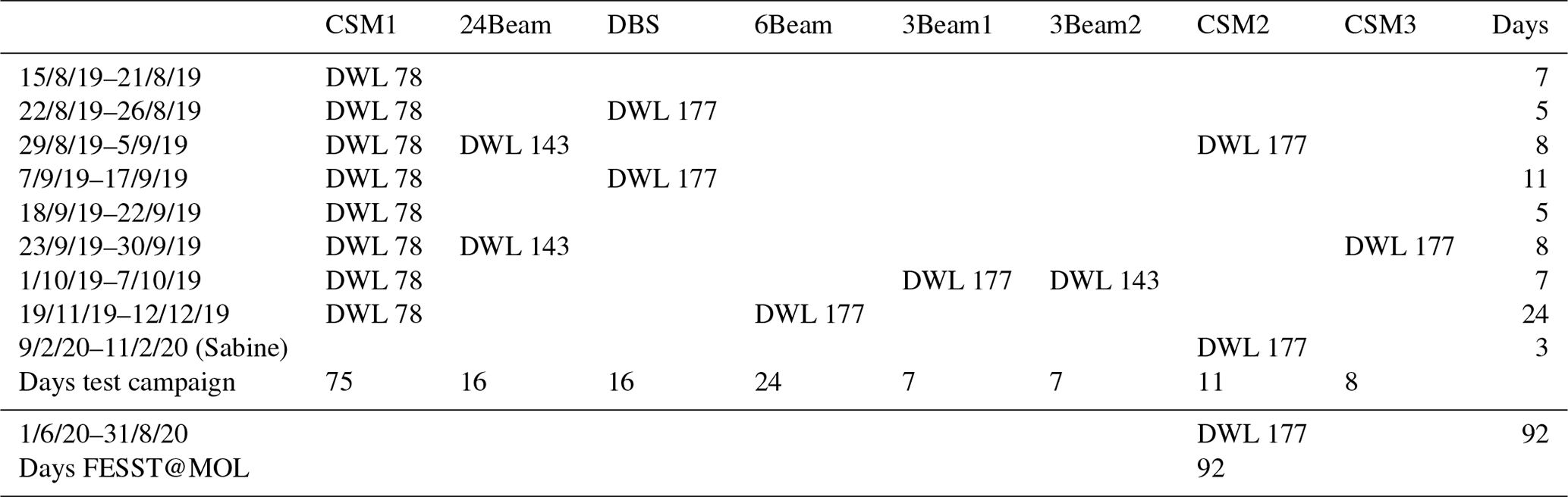
The configurations were operated as illustrated in Table 2. The test campaign began in late summer 2019 and continued through autumn 2019. Extratropical cyclone Sabine in February 2020 is the most significant event in our observation period. Although this event falls in 2020, it is likewise considered part of the test campaign in the later analysis. The number of days shown does not exactly reflect the observation period, as the configurations were switched during the day and also some observations in the daily files were truncated at the beginning or end of the day. As the sonic anemometer does not provide valid observations for north-northeast winds, these situations are missing in the comparison.
Table 2Configuration time schedule (in day/month/year) for the DWLs used.
2.4 Noise filtering
Typically, a DWL wind retrieval begins with a preprocessing of the observations that filters out noise. There are several approaches that use the signal-to-noise ratio (SNR) to separate useful and noisy measurements (e.g., Pearson et al., 2009; Barlow et al., 2011; Schween et al., 2014; Päschke et al., 2015). By comparing Doppler velocities with their SNR values, these approaches yield an SNR threshold below which measurements should be discarded. The threshold is given at the highest SNR value at which the Doppler velocities start to behave uniformly distributed over the entire range of theoretically measurable Doppler velocities, i.e., for our measurements roughly in the range of [−20 m s−1, 20 m s−1] whereby 20 m s−1 denotes the approximate Nyquist velocity. This change in the distribution behavior is most significant for direct measurements of vertical velocities because they usually take values close to zero.
However, we have found that filtering by an SNR threshold is not useful for some of our DWL configurations, especially for the quicker continuous scanning modes. Here, a high number of observations is achieved by emitting a relatively small number of pulses, which are then, however, associated with lower signal-to-noise ratios. If a threshold were introduced and only the observations with SNR values below it could be assumed to be noise-free, many measurements would be discarded. Nevertheless, noisy values can also be observed for the CSMs over the entire SNR range, which is why a rigid threshold value does not seem appropriate. In addition, threshold filtering always has the problem that too many measurements with reasonable Doppler velocities are eliminated.
As an example, Fig. 4 illustrates all SNR values measured with CSM2 on 2 September 2019 against their Doppler velocities. Here, it should be noted that the elevation angle is 62∘ so that the vertical wind is not measured directly. One can assume, however, that the very high absolute Doppler velocities correspond to noise. In this case, it is appropriate to detect noise by absolute values that are above about 5 m s−1. The two vertical lines in Fig. 4 are examples for which an SNR threshold could be set, e.g., at −23 dB as done by Pearson et al. (2009) or at −18.2 dB as done by Päschke et al. (2015). Nevertheless, at any reasonable or calculable threshold, noise would still be present in the measurements filtered this way, even if we filtered at an even stricter threshold, i.e., at a vertical line that would be further to the right in Fig. 4. Conversely, it can be seen that a large proportion of the measurements are in a region where the SNR thresholds suggest unreliable values (purple region).
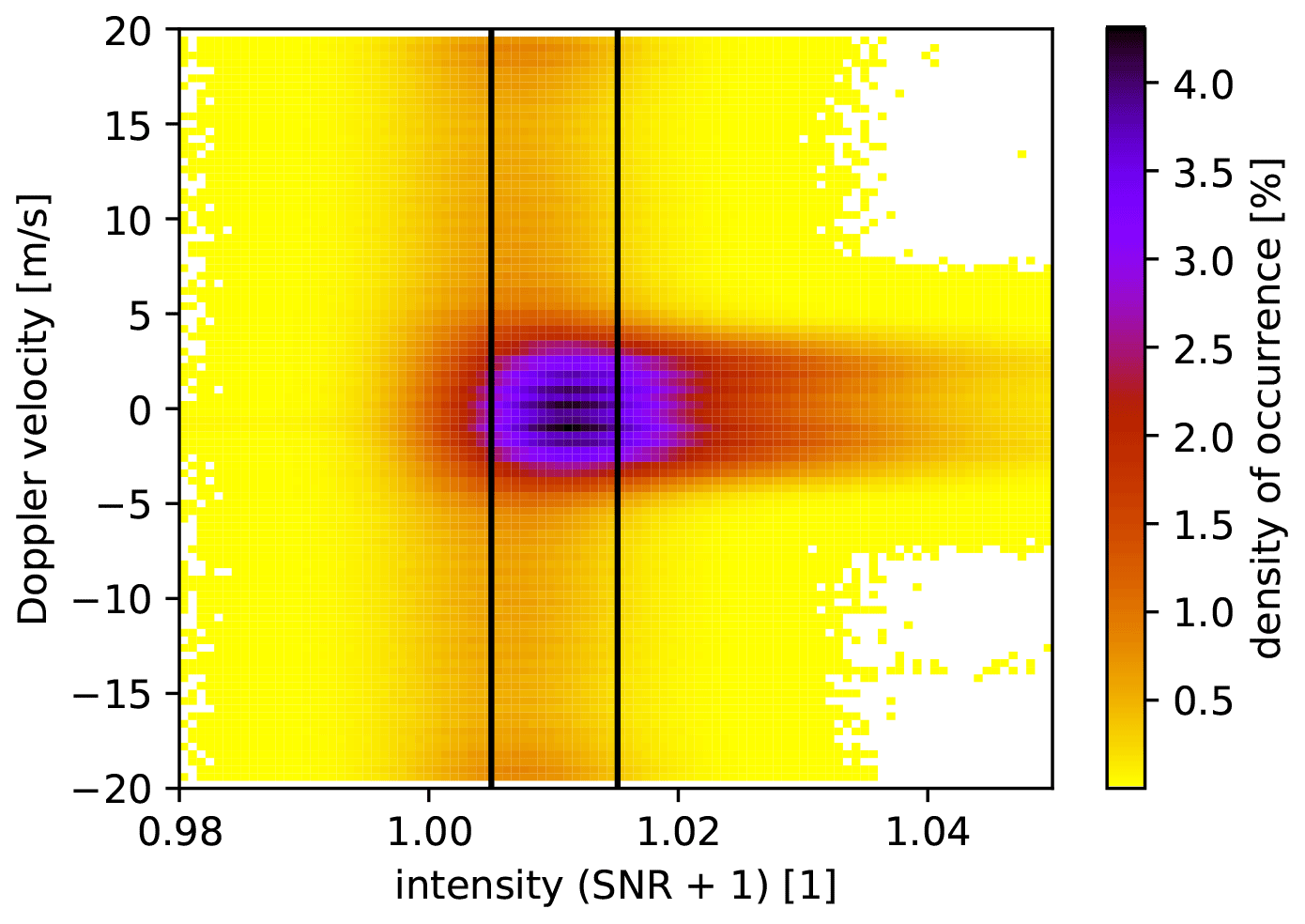
Figure 4Intensities (SNR + 1) vs. Doppler velocities on 2 September 2019 for all center-of-range gates during a 24 h observation period. The DWL is operated in CSM2 with a 62∘ elevation angle, and it produced 25 million measurements on that day. The area is divided into 100 × 100 bins, and the colors indicate the density of occurrence. The left vertical line corresponds to an SNR value of −23 dB and the right to −18.2 dB.
Instead of filtering the measurements in advance, we develop a method that initially includes all measurements but then iteratively filters out those measurements that deviate significantly compared to an intermediate fit solution such that they are detected as noise. This ensures that enough data are available to derive wind, in particular, gusts, which are in fact based on very few measurements. Simultaneously, the iteration incorporates thresholds that terminate the retrieval procedure if the set of measurements is too inconsistent and conditions prevail under which the wind vector cannot be derived. The complete iteration procedure is explained in more detail in the next section, as it is integrated in the retrieval.
The following calculations can be made for measurements performed during a specific time window, such as a 10 min interval, or based on measurements during a single DWL cycle. The number of single measurements per DWL cycle depends on the configuration used.
3.1 Wind vector fit
A measured Doppler velocity di is the projection of the wind vector vi along the measuring beam direction ai and satisfying the relation
with , where αi is the elevation and θi the azimuth angle of the ith of i=1…n consecutive Doppler velocity observations at a certain height. The instrument-induced observation errors are ϵi, which are assumed to be independent and normally distributed with zero mean and variance . The different Doppler velocities di all originate from different beams and thus from different wind vectors vi. Since the measurements are made sequentially with changing azimuth angle, there is not only a spatial but also a temporal difference, which is reflected in the vi. However, we assume that the wind field is homogeneous and each vi in the given time window, i.e., including the single DWL cycle, is the realization of one multivariate normally distributed random variable:
with mean wind vector v0 and three-dimensional covariance matrix Σ. The homogeneity assumption may be violated over complex terrain or during long time intervals. The different vi are assumed to be independent, which is another strong assumption and should be scrutinized by a DWL user as it ignores spatial and temporal correlations.
With different realizations vi, i.e., with consecutive measurements at different viewing angles θi and αi in a certain time window, the underlying values v0 and Σ could be estimated. The Doppler velocities di then are the linearly transformed wind vectors (i.e., projection on beam direction in Eq. 1), with an error variance that represents the observation error ϵi as well as the projected wind vector variability. They are normally distributed according to
We now assume that the wind vector variability is isotropic, i.e., the deviations of the individual vi from v0 are identically distributed in all spatial directions. Then the projection of the covariance matrix is independent of the direction ai and
The variance of di is thus a combination of the measurement error and the projected wind variability, i.e., the representation error. The likelihood function L for measured Doppler velocities di then reads
where is the combined variance and is the probability density function of a Gaussian distribution with expectation μ and variance σ2. Storing the n different beam directions ai row-wise in a n× 3 matrix A and the Doppler velocities in an n-dimensional vector d yields the maximum likelihood estimate (MLE) for , which is
Thus, is the least-squares fit over all measurements n within one single DWL cycle or within a respective time window. Note that we need at least three independent beam directions for the inversion of ATA. The residuals can be used to estimate σ2. For this, we use the unbiased estimator, i.e., the denominator n−3 instead of n to account for the degrees of freedom used to estimate the components of , which leads to
In the case of exactly three measurements the estimation of the variance is not possible. The corresponding standard deviation is equivalent to the root mean squared error (RMSE) and gives a measure of the fit performance.
3.2 Distribution of the estimator
With all the assumptions, the residuals are Gaussian-distributed with zero mean and variance σ2. The latter results from the assumption that the variability of the wind vector vi and the Gaussian observation errors ϵi are independent. Under the assumptions above, the distribution of the estimator is multivariate Gaussian-distributed. The expected value of is given as
The expectation value estimator is therefore unbiased. The variance of is
Both moments are derived in detail in Appendix A. Note that and the number of rows increases proportionally with n. One important assumption behind the covariance estimate of is that vi and v0 are independent of each other and the number of independent observations (i.e., degrees of freedom, DOFs) is n−3. This is definitely not the case, since the number of effective DOFs nef is much smaller than n−3, and therefore σ represents a lower bound of uncertainty. If we now assume that the estimate is based on substantially fewer independent measurements, we need to introduce a correction factor and estimate the covariance matrix with an effective nef instead of n−3, reading
Here, the estimate in Eq. (7) is used, and the nef needs to be specified depending on the desired time window of the retrieval.
3.3 Iterative retrieval update
Our retrieval aims at the estimation of two variables vm and vg. The 10 min mean wind velocity vm is estimated according to Eq. (6) over all n10 beams within a 10 min interval. The wind gust peak of a 10 min interval vg is the maximum of wind estimates, each derived from measurements along a single DWL cycle with nc observations, again using Eq. (6).
As discussed before, the noise in DWL measurements is uniformly distributed over the measurable Doppler velocity range and therefore distorts the estimation of . This is the case when is particularly large. For example, pure noise with uniformly distributed observations within [−20 m s−1, 20 m s−1] would yield an estimate of m s−1. Our retrieval procedure aims to filter out the Doppler velocity measurements di that are dominated by noise in an iterative process. To this end, we define a threshold u1 for at which the is assumed to be dominated by noise, as well as a minimum number q of measurements di that should be included in the estimation of . If , then is not accepted and the r measurements with the largest absolute residuals ei are removed. Provided that the number of remaining di is not less than q, is estimated again. Otherwise should be regarded as dominated by noise and set to not available (n.a.). However, we introduce a second threshold u2, which is more tolerant and accepts if even though . This second threshold is a higher bound at which sufficient confidence in the result has already been achieved, and the first threshold is a lower threshold that allows further improvement of the estimate when enough data are available. Note that the parameters u1, u2, r, and q are different for the two wind variable estimates vm and vg.
The iteration procedure is displayed in Fig. 5. In the upper right, the parameters are displayed for both vm and vg. The termination criterion u1 is m s−1 in both cases. For vm the second threshold is u2=3 m s−1. Since the single-cycle estimates of v0 rely only on very few di, we do not let u2 be more tolerable, i.e., m s−1. We in turn require that at least 66 % of the measurements are included for the single-cycle iteration, while q=50 % is sufficient for the 10 min mean wind. The number r of discarded measurements per iteration is 5 % for the 10 min wind and one for the single-cycle estimates. The set thresholds are intended to provide a clear distinction between observations that are too noisy and those which are usable. Nevertheless, it is possible to tune these values, but this is beyond the scope of this work.
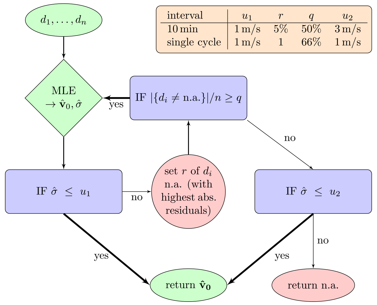
Figure 5Schematic flowchart of the DWL retrieval with the main steps to determine the wind vector estimate . All measurements from a given height and in a given time interval pass through the iteration loop. “If” statements (blue) use thresholds (u1, u2, and q) to decide whether to set n.a. values (red) or pass wind-fit data (green). The thresholds depend on whether the time interval is 10 min or consists only of the measurements of a single DWL cycle (see orange box).
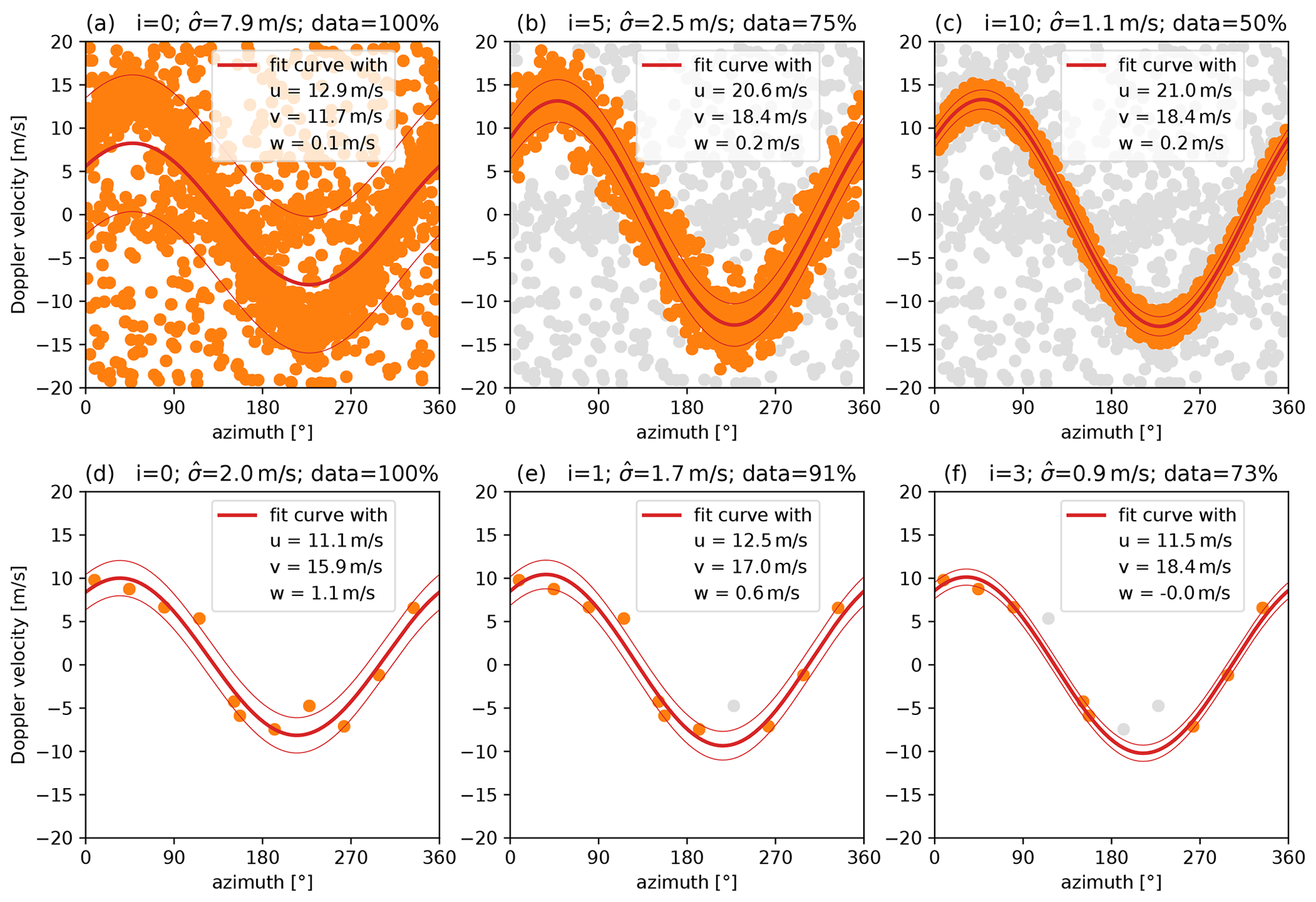
Figure 6Different steps (i) of the retrieval for 10 min mean wind (a–c) and for the wind of a single DWL cycle (d–f). The sinusoidal projection (fit curve with) of the fitted wind vector (u, v, and w) is shown in thick red, with a standard deviation tube around it (, red). Observations used for the displayed wind vector fit are orange, and omitted observations are grey. Panels (c) and (f) display the fits that are finally returned. The examples are from a DWL operated in CSM2 on 10 February 2020 and from measurements at 808 m (a–c) and 225 m (d–f).
Figure 6 illustrates the principle of the iteration procedure. Figure 6a to c illustrate different iteration steps for the estimation of a 10 min mean wind and Fig. 6d to f for the estimation of a wind of one single cycle. In the upper panels, the iteration runs for 10 complete iterations, discards 50 % of measurements, and ends with that falls between 1 and 3 m s−1. Hereby, Fig. 6b shows the first intermediate state in which the retrieval would already accept the estimate because falls below 3 m s−1, but then continues improving until less than 50 % of measurements are used, as in Fig. 6c, or the more rigorous threshold u1=1 m s−1 would be reached. In the lower panels, one measurement is discarded in each iteration and the retrieval only returns a result that falls below 1 m s−1, as in Fig. 6f, since the values in Fig. 6d and e are both too high.
Combined, the retrieval then provides the 10 min mean and a sequence of cycle-based individual winds within 10 min. The gust peak can then be determined from the cycle-based winds. Here another check is included to prevent susceptibility to unrealistic outliers. Those cycle-based winds that deviate in absolute speed by more than 1 m s−1 from all others within the 10 min sequence are removed. This affects outliers of the two bounds, so both the strongest and weakest gusts are checked. If at least 50 % of the cycle-based winds still exist and also the 10 min wind is not n.a., the gust peak is then determined to be the maximum of all remaining cycle-based winds within 10 min (and the minimum is defined as the minimum of the cycle-based winds).
3.4 Estimation of uncertainty
The covariance estimate in Eq. (10) includes the estimated value . If is derived from the residuals that remain after the iteration process to estimate , then the uncertainty is greatly underestimated. However, the inclusion of all measurements would overestimate the uncertainty. To account for uncertainty in the eliminated observations that is consistent with our statistical model, we assume that these residuals represent the truncated part of a normal distribution. Therefore, the variance estimated from the non-eliminated measurements must be corrected accordingly. Let p be the percentage of discarded measurements, i.e., truncated values. If p is the fraction of two-sided truncated values at symmetric thresholds a and b, then the threshold a and b are given by and , i.e., the and quantiles, respectively, where Φ is the cumulative distribution function and ϕ the probability density function for the standard normal distribution of the original (non-truncated) values with parameters μ and . Following Johnson et al. (1994), the relation between the variance of the truncated variable and non-truncated is
This can be used to re-scale and approximate a corrected covariance matrix towards
We use the corrected covariance matrix as the estimate of the wind uncertainty for both the 10 min mean wind and the wind of a cycle. The uncertainty of the gust peak is associated with the covariance matrix of the corresponding maximum. Determining nef is discussed in Sect. 4.3.
The results in Sect. 4.1 are obtained from DWLs operated in different configurations from the end of summer 2019 to the beginning of winter 2019–2020, with additional consideration of 3 d of cyclone Sabine in February 2020. Moreover, cyclone Sabine is the subject of Sect. 4.2. Based on these results, we performed measurements in the fast CSM2 over several weeks in summer 2020, for which performance statistics were derived and are presented in Sect. 4.3.
4.1 Comparative test study
Figure 7 shows scatterplots of the 10 min mean horizontal wind from the sonic anemometer versus the DWL retrieval for the eight configurations in Fig. 3. In order to measure the quality of the retrieval, we use the RMSE, the bias, and the coefficient of determination R2 between DWL retrieval and sonic measurement. All eight configurations produce only minor biases ranging from −0.13 to 0.14 m s−1. The CSM1 in Fig. 7a is based on a large sample since it has been tested almost continuously. Apart from some underestimations at low wind speeds, here the wind is observed with small RMSE (0.41 m s−1), high R2 (0.97), and negligible bias (0.04 m s−1). For the 24Beam in Fig. 7b, some DWL outliers can be recognized, which can be explained by the relatively steep elevation angle. The outliers result from the fact that the linear interpolation of the Doppler velocities fails at 90.3 m because the involved Doppler velocities of the lowest range gate centers are too close to the DWL. Close to the DWL, the transmitter and receiver field of view do not completely overlap. Therefore, the Doppler velocities originating from the lowest range gates should be discarded and those of the following ones are at least noisier. The amount of full overlap is instrument-dependent, and the obvious outliers show that the Doppler velocities cannot always be considered reliable at 75 m of radial distance from the DWL, i.e., at 72 m a.g.l. for 75∘ elevation, which corresponds to the distance to the third center-of-range gate. In fact, a comparison with the results of range gates centered at 101 m a.g.l. (fourth center-of-range gate) would give a better result (not shown). These outliers lead to a higher RMSE (1.12 m s−1) and a lower R2 (0.8). DBS in panel (c) and 6Beam in panel (d) both exhibit low RMSE values (0.29 and 0.34 m s−1, respectively) and R2 values close to 1 (both 0.98), indicating a low scattering between sonic anemometer measurement and DWL retrieval. The 3Beam configurations in Fig. 7e and f perform very similarly, and the scatterplots are based on parallel measurements in October 2019. The quicker configuration actually performs slightly better in terms of diagnostic variables (RMSE with 0.38 m s−1 < 0.48 m s−1 and bias with |0.0 m s < m s), although this is mainly due to the one high DWL outlier at low sonic anemometer wind in Fig. 7f. The two fast continuous measurement modes CSM2 and CSM3 yield narrow scatterplots in Fig. 7g and h, respectively, with low RMSE (0.43 and 0.34 m s−1), little bias (−0.1 and 0.12 m s−1), and low variation in terms of R2 (0.98 and 0.99).
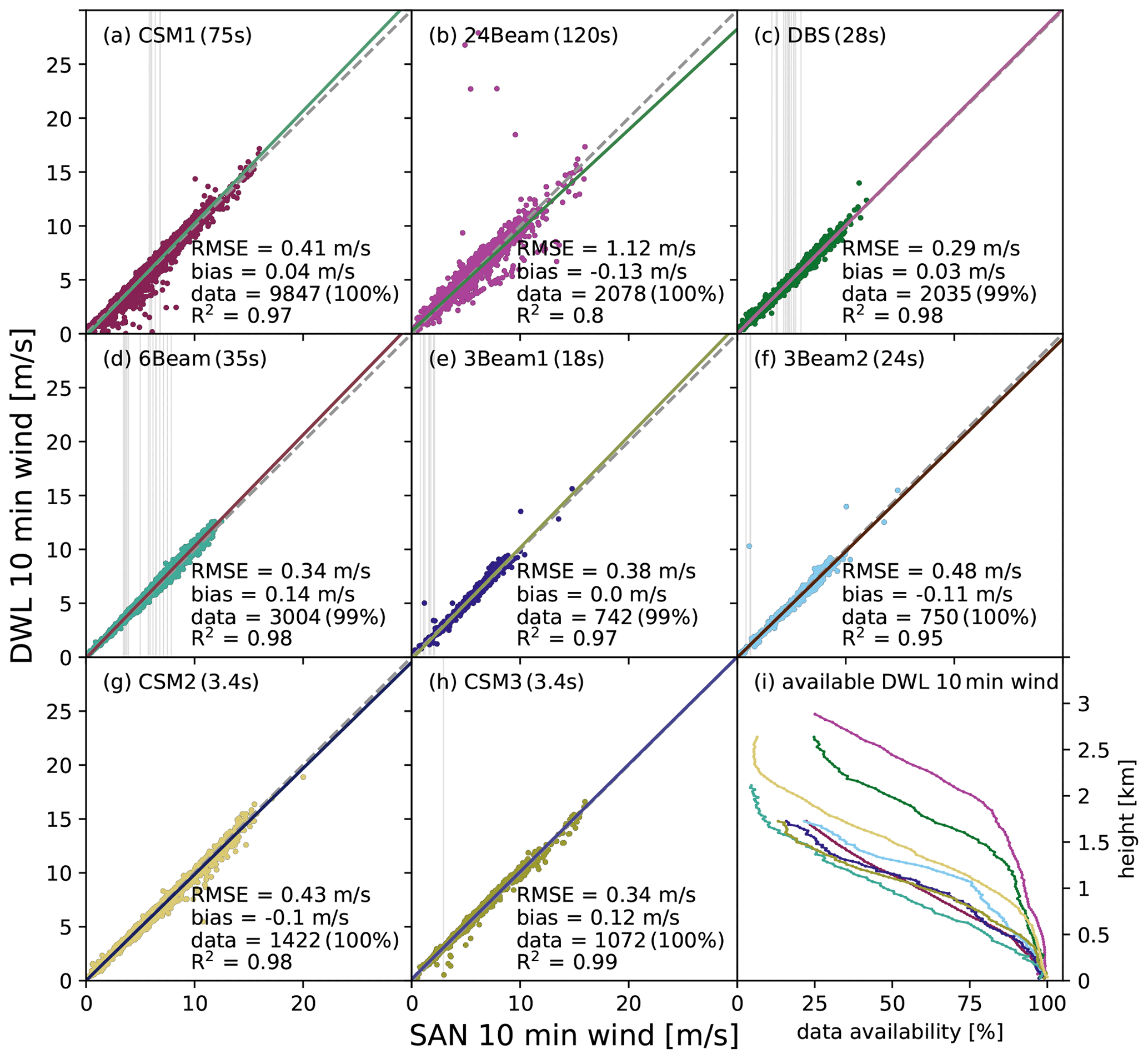
Figure 7Scatterplots of 10 min mean horizontal wind from the sonic anemometer (SAN) versus DWL for the eight different tested DWL configurations at 90.3 m. Colors and letters (a)–(h) correspond to the configurations shown in Fig. 3 with the measurement configuration schedule given in Table 1. For each panel, the colored linear fit line, the root mean squared error (RSME), the bias, the involved data, and the coefficient of determination (R2) are given. The parameter data indicate in parentheses the fraction of situations in which the DWL retrieval returned valid wind values. Grey vertical lines indicate sonic anemometer measurements with missing corresponding DWL results. Panel (i) shows the DWL data availability against height with colors per configuration as in panels (a)–(h).
The DWL data availability at 90.3 m is close to 100 % for all configurations. Data availability with height depends mainly on the elevation angle; i.e., the steeper the angle, the higher the amount of retrieved wind data at a certain height. For the same elevation angles, the configuration with more pulses emitted per beam tends to achieve higher data availability for a given height (compare DBS and CSM2 with 3Beam2 and 3Beam1, respectively). The 6Beam has a comparatively low data availability in the vertical profile. However, it should also be mentioned here again that the data are not directly comparable because the observation period and duration are different. The 6Beam observation period fell in November–December, which is a period with different atmospheric conditions, especially more precipitation and more frequent occurrence of low clouds and fog, which can interfere with the DWL observations. All in all, the configurations seem to be able to properly monitor the lowest 1 km above the ground and thus the atmospheric boundary layer.
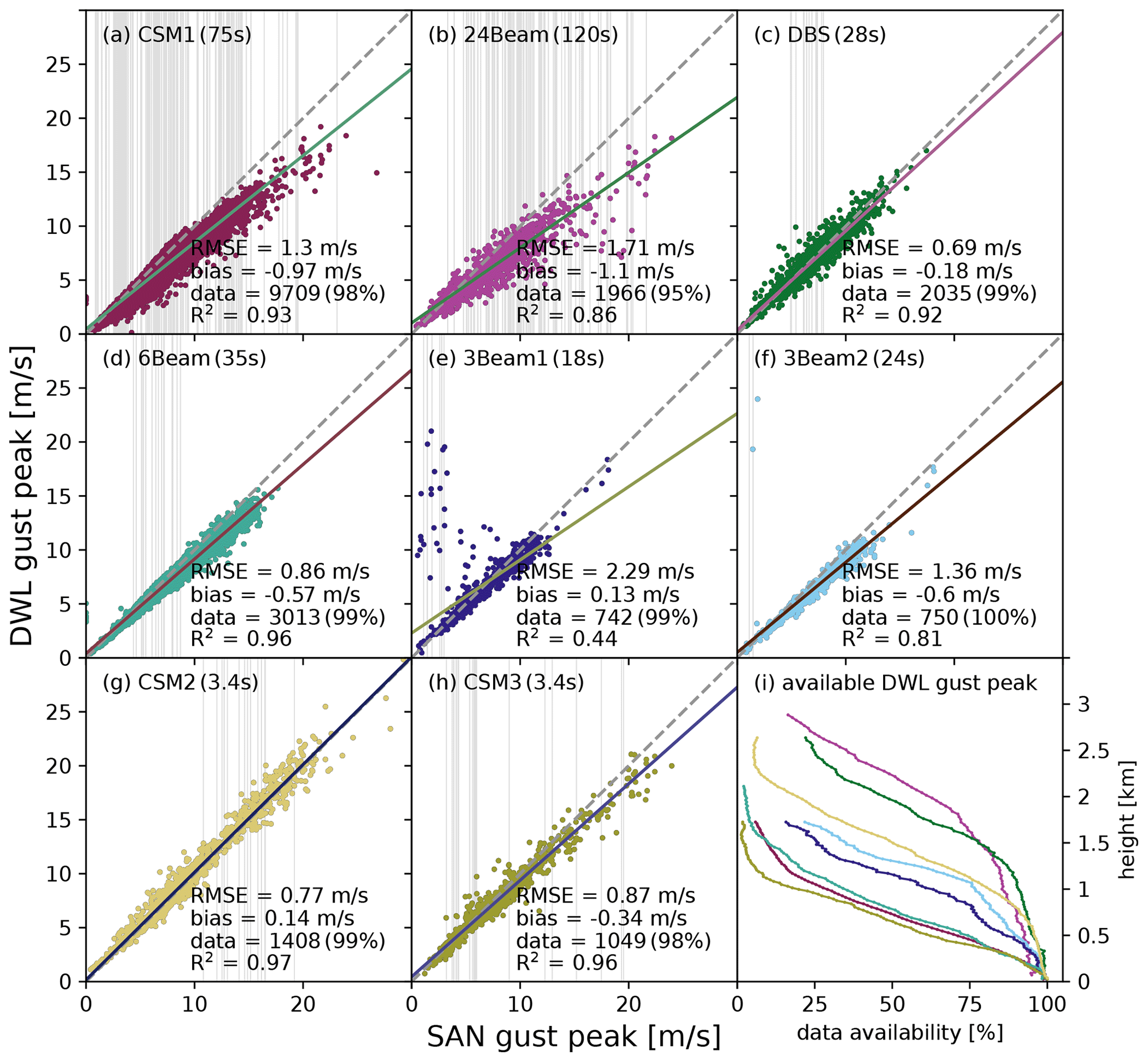
Figure 8Scatterplots of the sonic anemometer (SAN) gust peak (3 s in 10 min) versus the DWL gust peak (gust duration as indicated per panel in 10 min) for the eight different tested DWL configurations at 90.3 m. The further explanations are the same as in Fig. 7. Panel (i) shows the data availability against height with colors per configuration as in panels (a)–(h).
Figure 8 shows scatterplots of the 10 min gust peaks from the sonic anemometer versus the DWL retrieval for the eight configurations. The performance of the configurations depends strongly on the time required per DWL cycle. The two slow configurations, CSM1 and 24Beam, in Fig. 8a and b underestimate the gust peaks (biases of −0.97 and −1.1 m s−1). Here, the CSM1 yields a good coefficient of determination (0.93) and could still be useful with an adequate bias correction, while the 24Beam results appear to be too variable, especially for the highest gust peaks. DBS and 6Beam appear to be quite accurate in Fig. 8c and d, with lower RMSEs (0.69 and 0.86 m s−1). However, their observation periods coincide with weak gust peaks, so their performance is not entirely clear. At least the highest gust peaks determined for the 6Beam are below the intersection line, suggesting that more extreme gust peaks tend to be underestimated. Here, a bias correction or rescaling could also provide useful results. Obviously, in too many cases, the 3Beam1 in Fig. 8e fails to detect the actual low gust peaks recorded by the sonic anemometer. In contrast, though, the few actual high gust peaks are detected very well. The parallel-measuring 3Beam2 in Fig. 8f provides only two significant overestimates but is less capable of catching the highest gust peaks, although it still gives reasonable results. Both 3Beam configurations thus provide worse performance values (e.g., RMSEs of 2.29 and 1.36 m s−1). The fast CSM configurations are closest to the gust definition of a wind peak lasting at least 3 s since it takes 3.4 s to complete their measurement cycles. The two scatterplots in Fig. 8g and h show very high agreement between the measured gust peaks from the DWL and sonic anemometer. Although the performance values (e.g., biases of 0.14 and −0.34 m s−1) are comparable to DBS and 6Beam, the measurements include gust peaks above 20 m s−1. Moreover, for the two elevation angles of 62∘ and 35.3∘ studied here, high gust peaks were observed whose points were also close to the intersection line. The linear fit for CSM2 is nearly perfect at the line of intersection, while the flatter CSM3 has a fit with a slightly lower slope. At the steep elevation angle, the observation cone at 90.3 m has a diameter of almost 100 m and at the lower elevation angle a diameter of 255 m. The smaller the studied volume, the more likely one particular gust can be assumed to be detectable in the observation cone. In terms of RSME, the CSM2 provides a lower value (0.77 m s−1 compared to 0.87 m s−1).
The availability of the wind data is generally lower than that of the mean horizontal 10 min wind, but again the same elevation angle dependence is evident; i.e., the higher the elevation angle of the configuration, the more data are available at given height. Consideration of all these factors, combined with relatively good data availability in the vertical for an elevation angle of 62∘, leads to the decision to use the CSM2 for the later observation periods.
4.2 Extratropical cyclone Sabine
Storm Sabine was an extratropical cyclone with severe impacts throughout Europe. Gale-force winds led to the collapse of large sections of the transport network in Germany. The highest gust peak in Germany of about 49.1 m s−1 was measured at Feldberg in the Black Forest (Haeseler et al., 2020). For Falkenberg's sonic anemometer at 90.3 m, the highest gust peak was observed on 10 February 2020 at 29.3 m s−1, which was the highest value during the observation period of our study.
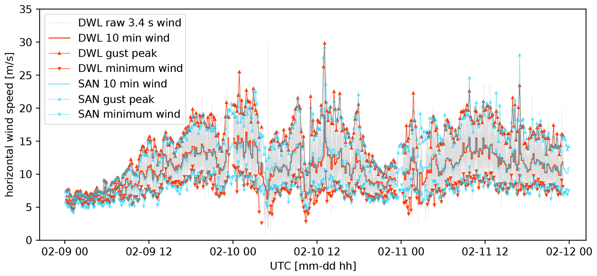
Figure 9Time series of wind speeds during extratropical storm Sabine on 9–11 February 2020. Both the DWL operated in CSM2 (red) and sonic anemometer (SAN, cyan) winds are shown. The triangles indicate the 10 min gust peaks and wind minima, the thicker step-like lines indicate the 10 min mean horizontal wind, and the light grey line shows the results for all processed DWL cycles. Very good agreement between the data means that markers and lines completely overlap. Note that due to outlier filtering, not all cycle maxima and minima match the gust peak and wind minimum values, respectively.
Figure 9 shows the observations during the 3 d evolution of storm Sabine at 90.3 m in Falkenberg for both a DWL operated in CSM2 and the sonic anemometer. It can be seen that the wind speed increases throughout the day on 9 February, reaching the overall highest values around noon on 10 February 2020. During the following night, the wind intensity decreases, becoming high again on 11 February and decaying afterwards (on 12 February 2020, which is not shown). The complete time series of the sonic anemometer is convincingly reproduced by the DWL in terms of the 10 min mean wind, the wind minima, and the gust peaks. There are three periods when the DWL underestimates the minimum wind and at the same time tends to underestimate the 10 min mean wind. Simultaneously, however, the gust peaks are adequately reproduced. Furthermore, the strongest gust is calculated to be 29.8 m s−1. It deviates by only 0.5 m s−1 from the sonic anemometer measurement, thus providing a convincing result. For the other high gust peaks, in some cases larger deviations are registered, although these do not show any systematic underestimation or overestimation. In addition, the horizontal wind values of the individual cycles are shown, which cover the ranges of minimum wind to gust peak. As shown by the discrepancy of some DWL cycle winds and the returned DWL gust peaks or wind minima, the implemented outlier detection works, and mostly unrealistically high or low values are filtered out before peaks and wind minima are determined.

Figure 10Color-coded wind barbs for gust peaks during extratropical cyclone Sabine on 10 February 2020 from the DWL operated in CSM2. (a) Results for a retrieval with classic SNR filtering at −18.2 dB and MLE. (b) Results without SNR filtering and iteratively improved MLE as developed in this study. In both approaches, the gust peak per 10 min is only given if at least 50 % of the DWL cycles obtain valid values.
To assess the performance of the retrieval in terms of vertical resolution of gusts, we compare our new retrieval to a classic retrieval exemplified for 10 February 2020 in Fig. 10. A classic retrieval is not designed to derive wind gusts but usually to determine a mean wind, so the filtering can eliminate more measurements. Here, by classic retrieval, we mean classic threshold filtering followed by MLE, which determines the wind vector from the remaining measurements of each DWL cycle. Thus, similar to the new approach, we obtain wind vectors from which wind gusts can be derived. Hence, the calculation is not iterated and all remaining observations are used. The wind gusts in Fig. 10a are from this classic retrieval with the cycle-based MLE for prefiltered Doppler velocities at an SNR threshold of −18.2 dB according to Päschke et al. (2015). For each MLE, 66 % of available Doppler velocities are required, and for the calculation of the 10 min gust peak, at least 50 % of the individual cycles must have been processed (valid for both approaches). This procedure is a classic noise filtering, but with a calculation based on very few observations. Figure 10b shows the result of our proposed retrieval. Both retrievals used the same measured Doppler velocities from a DWL operated in the CSM2 configuration. The new retrieval has significantly higher data availability. The gust peaks indicated by the classic retrieval are very similarly covered by the new retrieval, which shows that the new retrieval eventually uses the same observations that the classic threshold filtering would leave. In Fig. 10b, the additional obtained gust peaks fit coherently into the overall impression of the storm. This means that the new retrieval does not distort results that are also produced by rigorous filtering. On the other hand, it is also observed that the inclusion of too many observations that are potentially noisy does not disturb the retrieval result.
This example is a satisfactory demonstration of the usefulness of the CSM2 configuration in combination with the new retrieval in terms of data availability of coherent gust peaks. Exactly such extreme events are to be monitored precisely by the DWL. For this reason and because of the statistics from the whole comparative test campaign, we set up a DWL in CSM2 throughout the summer of 2020.
4.3 Summer 2020
We extend the validation to a longer time period to look at a large sample of data. Figure 11 provides the comparative statistics for observations from summer 2020. The 3 months were relatively warm and dry for Brandenburg, while in addition weak winds from the north-northeast prevailed frequently. This is reflected in the data availability for the comparisons, which is reduced by 13 % due to the shading effect of the tower on the sonic anemometer. The DWL, in contrast, conducts wind measurements for almost the entire period. The vertical lines denote the sonic anemometer measurements in which the DWL does not process any winds and which are less than 1 % for both wind products. In particular, neither high mean winds nor strong gust peaks are missing in the processed data of the DWL. The comparison of the 10 min mean winds confirms that the CSM2 is suitable for deriving a mean wind at 90.3 m. Both the appropriate linear fit and the measures of spread, i.e., RMSE (0.4 m s−1) and the coefficient of determination (0.98), emphasize the suitability of the retrieval and the used configuration for retrieving a conventional DWL wind product. The comparison of the gust peaks provides high coincidences. The scatter is larger compared to the mean wind, as a small-scale process is more difficult to capture. As for the discussed test period, the CSM2 does not introduce a systematic error, and larger deviations are rare. Except for 18 cases, gust peaks are calculated for the situations in which the 10 min mean wind is processed. It can therefore be assumed that iterative filtering eliminates noise in a relatively similar way, regardless of whether the mean wind vector or the instantaneous wind value of an individual measurement cycle is considered. Although it may happen that a high gust peak could generate Doppler velocities that are considered noise in the derivation of the mean wind, it is precisely then that it is very practical to filter for both wind products independently. On the one hand, Doppler velocities of an individual gust peak that are significantly different to Doppler velocities belonging to the mean wind are negligible in the mean wind retrieval as these would be only few of the total amount of observations within 10 min. On the other hand, that gust peak is recognized as such in the single cycle-based retrieval, provided it is clearly visible in the few measurements within one single DWL cycle. Thus, the noise filtering seems to work effectively with respect to the requested wind product.
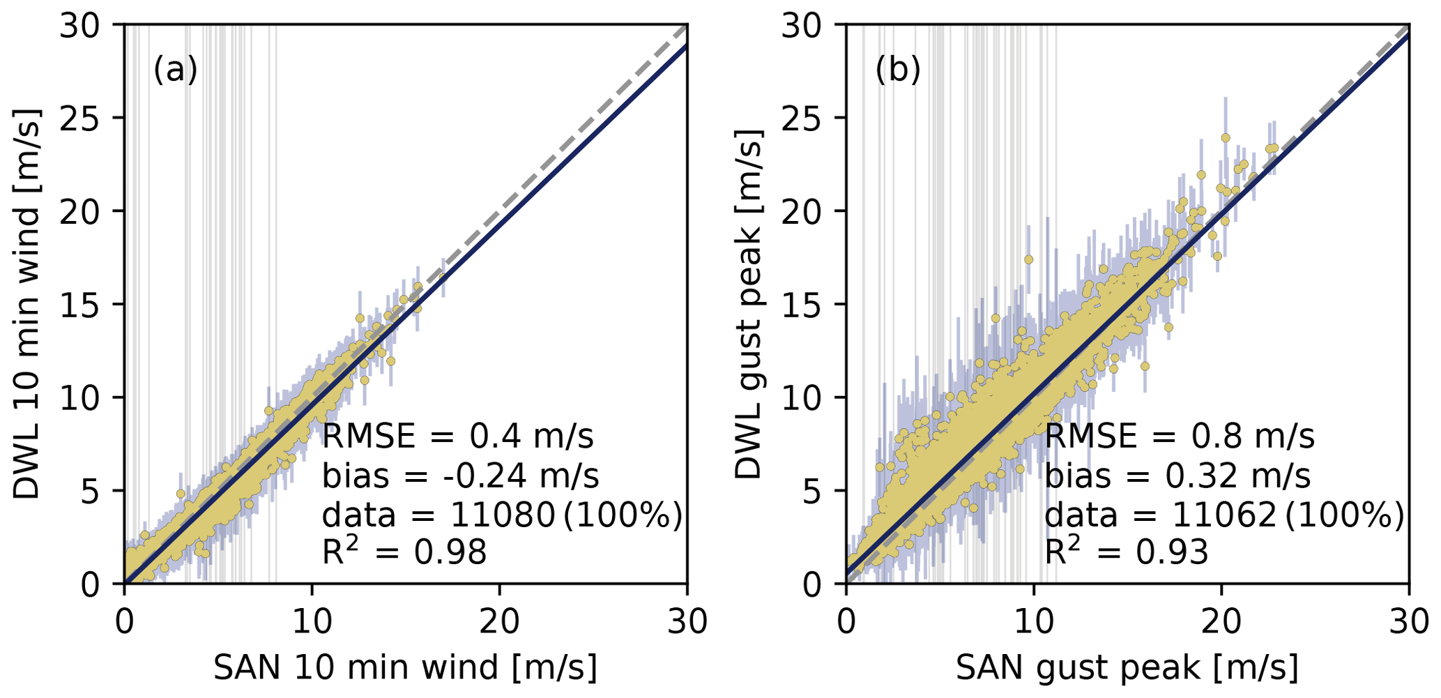
Figure 11Scatterplots of sonic anemometer vs. DWL wind retrieval during the period 1 June to 31 August 2020 at 90.3 m. (a) Scatterplot of 10 min mean horizontal wind from a sonic anemometer (SAN) versus the DWL operated in CSM2. (b) Scatterplot of the SAN gust peak (3 s in 10 min) versus the DWL gust peaks (3.4 s) operated in CSM2. The diagnostic numbers are explained in Fig. 7. The estimated DWL standard deviation of the horizontal wind or gust peak is shown with vertical bars derived from the estimated covariance matrix with nef=12 (a) and nef=2 (b), respectively.
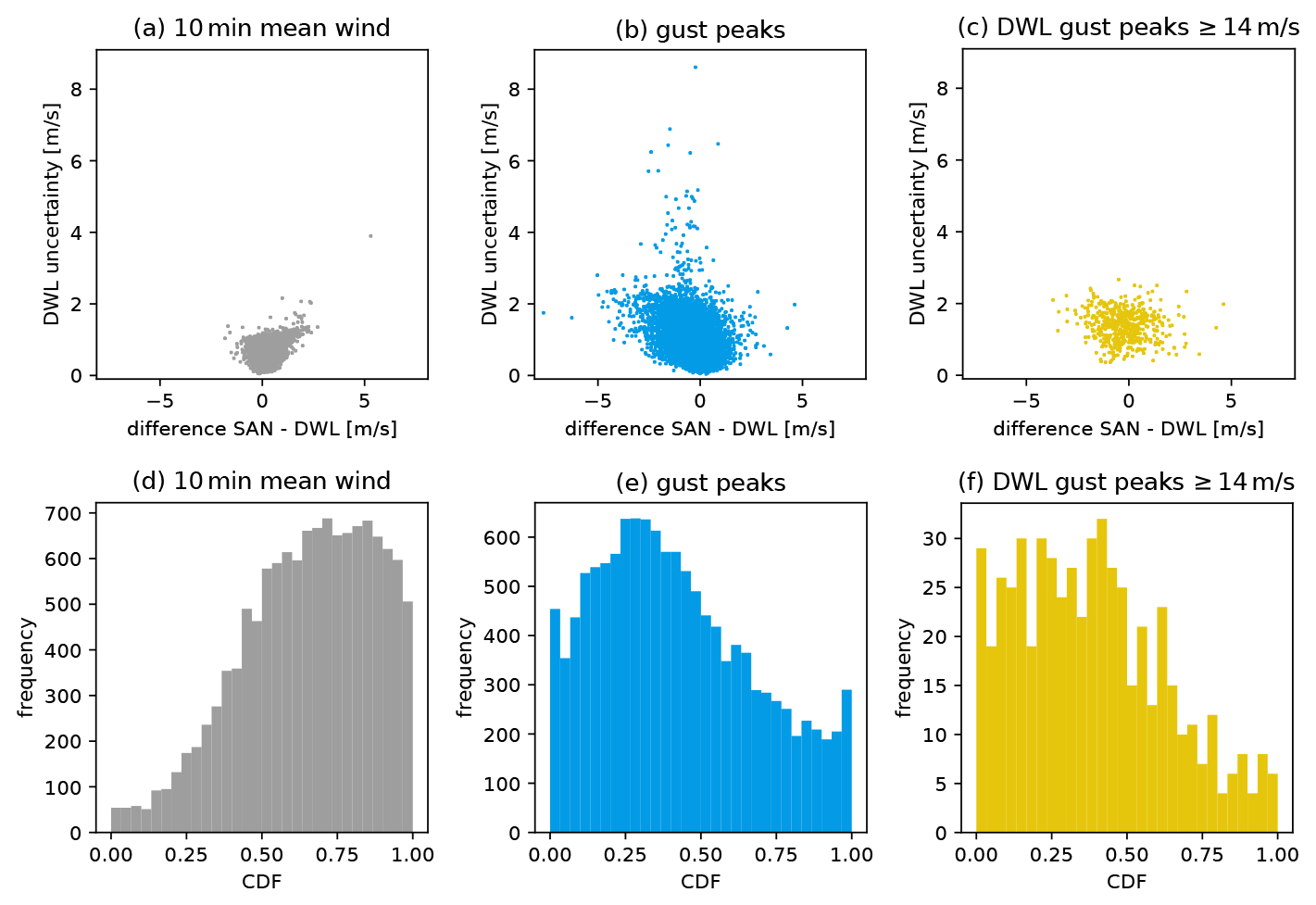
Figure 12Examination of uncertainty. Panels (a)–(c) show comparisons for the differences of the sonic anemometer (SAN) and DWL wind values against the estimated DWL uncertainty. Panel (a) displays the results for the 10 min mean horizontal wind, panel (b) for the gust peaks, and panel (c) for only cases in which the DWL gust peaks exceed 14 m s−1. Panels (d)–(f) show the rank histograms for the retrieved DWL wind and its corresponding uncertainty; panel (d) addresses the 10 min mean horizontal wind, panel (e) gust peaks, and panel (f) the gust peaks exceeding 14 m s−1. Each histogram shows the frequency of the Gaussian wind cumulative distribution function values, evaluated at the sonic anemometer observations. A perfect model would show equally distributed frequencies.
The scatterplot includes the uncertainty estimates for the horizontal winds. The standard deviation, shown with two vertical bars for each point, should approximately cover the range by which the observation falls within 68 % probability for normally distributed random variables. The estimation of the uncertainty depends on the choice of the effective DOFs, i.e., nef from Eq. (12). We set nef=12 for the 10 min mean wind and nef=2 for the wind of a cycle, which is then also representative for the gust peak. Except for some outliers, the uncertainties for both wind products emphasize the agreement between the DWL and sonic anemometer, and larger deviations between them are usually associated with larger uncertainties. The two effective DOFs used here are a result of tests with different nef. For that, we used all available results from observations in the CSM2 configuration, i.e., also the measurements of the comparative test study. Figure 12 shows scatterplots for uncertainty estimates against the difference between sonic anemometer and DWL wind, as well as an assessment from a probabilistic point of view with rank histograms, namely for nef=12 and nef=2. In these rank histograms, the retrieval outcome is understood as expectation and variance parameters of a Gaussian cumulative distribution function (CDF), which is evaluated for the sonic anemometer observation. The histogram illustrates the frequencies of the different CDF values. An equally distributed rank histogram indicates a calibrated forecast, i.e., in which the uncertainty parameters of the distribution are neither underestimated nor overestimated. In Fig. 12a it can be seen that the 10 min mean wind is estimated to be very confident while also deviating relatively little from the sonic anemometer observation. Nevertheless, it is also recognizable that tentatively more winds are underestimated than overestimated. Such underestimated winds come with increased DWL uncertainty estimates, which becomes extremely noticeable in the case of one realization (see the upper left corner). Differences and uncertainty estimates are of the same order of magnitude, however. For the mean wind in Fig. 12d it is apparent that the sonic anemometer 10 min mean wind is over-proportionally often higher than the expectation value. Nevertheless, setting the effective degrees of freedom with nef=12 results in an appropriate order of magnitude for effective independence. Higher values for nef would reduce the estimates for uncertainty and contribute to a slight flattening of the rank histogram, but also lead to a more frequent occurrence of results around CDF=1 (i.e., cases of underestimated winds with simultaneously estimated confidence that is too high). Vice versa, a lower nef would yield uncertainties that are too high, producing a higher peak in the rank histogram. The skewness cannot be fixed with the modification of nef. Concerning the evaluation for gust peaks in Fig. 12b, it is again noticeable that the differences between the sonic anemometer and DWL are generally larger than for the mean winds. At the same time, however, the estimate for the uncertainty is also larger. Further, it is apparent that gust peaks tend to be overestimated by the DWL. Figure 12e confirms this impression because there are more evaluations of the sonic anemometer observation on the left side of the histogram. With nef=2 we set a reasonably low value in order not to underestimate the uncertainty. There are not many misunderstood outliers; i.e., there are not too many sonic anemometer gust observations that do not match the retrieval at all and whose CDFs are close to 0 or 1. Since the consideration of extreme gust peaks is of particular relevance, Fig. 12c and f show the assessment for gusts above 14 m s−1. This is the threshold value for the forecast at which warnings of gusts must be issued in Germany. No significant difference to the assessment of all gust peaks can be ascertained here. This confirms once again that strong gusts in our observation period do not present special difficulties for the new retrieval.
Within the framework of the FESSTVaL measurement campaign, we investigate various configurations with regard to their ability to observe 10 min mean wind and wind gust peaks. For this purpose, a retrieval is developed that can flexibly quantify wind and associated uncertainty for different averaging time intervals. Our noise filtering is meshed in the retrieval and is based on the assumption that noise is distinguishable from real measurements and can be removed iteratively. The retrieval proves to be suitable to process the 10 min mean wind for all tested DWL configurations. Besides the mean wind, the retrieval is used to process the wind of the single DWL cycles. The maxima of the single cycles within 10 min are considered to represent the wind gust peaks. Due to different settings, the tested configurations differ in the time required to complete all measurements of a respective cycle. A quick continuous scanning mode, the CSM2, proves to be successful for deriving gust peaks similar to those of a sonic anemometer at 90.3 m. This CSM2 provides 11 single radial Doppler wind measurements during one revolution of the DWL scan head, which is completed within 3.4 s and from which the wind vector is derived. Measurements with this configuration are performed during the passage of extratropical storm Sabine in February 2020. The strongest gust peak in the whole observation period was measured here and accurately reproduced. Comparison of the new retrieval with a classic approach showed significantly higher vertical data availability for the new retrieval. Although comparative measurements from other heights are missing, the results of this storm day example provide a coherent overall picture of the vertical wind gust profiles. The other configurations require a longer time to complete a measurement cycle and are therefore unsuitable for measuring wind gusts directly. However, it would be possible to scale the retrieved gusts to obtain values that are more comparable to the 3 s sonic anemometer results. In particular, the scaling method of Suomi et al. (2017) could be applied.
During the summer of 2020, we tested the CSM2 for a full 3 months. For both mean winds and gust peaks, we are able to cover almost the entire observation period for which usable sonic anemometer observations exist. Overall, the DWL and sonic measurements agreed with low RMSE (0.4 m s−1 for 10 mean wind and 0.8 m s−1 for gust peaks, respectively) and small biases (−0.24 and 0.32 m s−1); in addition, there are also no cases of strong gusts that the DWL retrieval has not identified. Finally, the estimated uncertainty of the retrieval is evaluated. The uncertainty estimates for mean wind and gust peaks are of the order of magnitude of absolute error with respect to the sonic anemometer. The mean wind is somewhat too often underestimated by the DWL, while the gust peaks are rather too often detected higher than the sonic anemometer. Apart from this asymmetry, these results are nevertheless satisfactory, because it also shows that the DWL distribution did not describe situations that do not match the sonic anemometer observation too often.
The uncertainty was correctly represented, but the use of an effective DOF is necessary. We have used different DOFs for requested winds, i.e., whether it was cycle-based or within 10 min, but there is still room for improvement. Our aim was to provide a reliable estimate, and its tuning is beyond the scope of this study. In particular, separate DOFs could also be appropriate for different weather situations, as well as for the different configurations, of which we examined only CSM2. We show how useful the CSM2 could be if operated at an elevation angle of 62∘. Using an elevation angle 35.3∘ gives results of similar quality. We have not systematically answered how to choose the optimal angle, which could be investigated further. The general advantage of the suggested fast CSM lies in the fact that it completes one measurement cycle within 3.4 s. To our knowledge, there is no comparable DWL scan configuration that performs a similar number of radial velocity measurements in such a short cycle.
The newly available FESSTVaL data set from summer 2021 offers further opportunities for detailed case studies and comparative studies involving several DWLs and airborne in situ measurements. The airborne measurements provide a reference for the quality of retrieval in higher layers. There are parallel DWL measurements in the same quick CSM configuration but at different locations, so the spatial evolution of gust structures can be analyzed. Here, the high-resolution time series of the wind vector generated with the retrieval offers the potential to study turbulence in detail. Thereby, it has to be shown whether the derived vertical wind is of comparable quality as measurements of a vertically pointing DWL. Steinheuer and Friederichs (2020) show that gust profiles can be derived from reanalysis data. This method can still be tested at various locations, which is now also possible with the means of DWLs. We hope that our retrieval lays the foundation for expanding the monitoring network for high-frequency wind measurements with DWLs for weather research and applications.
The expected value of holds the following.
Equations (A1)–(A3) are obtained by inserting definitions. Then the expectation is applied to vi and ϵi, and the matrices cancel out.
The variance of holds the following.
Equation (A9) arises by supplementing v0 with (ATA)−1ATA and rearranging. Then in Eq. (A12) the expectation value calculation is applied, exploiting the fact that observation errors ϵi are uncorrelated with each other and with the individual deviations from the mean wind (vi−v0).
The code is available at https://doi.org/10.5281/zenodo.5780949 (Steinheuer et al., 2021a).
The data are available at https://doi.org/10.25592/uhhfdm.9758 (Steinheuer et al., 2021b).
UL and FB, together with others, planned the FESSTVaL campaign. FB and CD were responsible for logistics on the site and performed the measurements. JS and CD developed the retrieval methodology with idea contributions from all others. JS coded the retrieval. JS, UL, and SF planned and structured the paper. JS and PF developed the uncertainty methodology of the retrieval. JS drafted the paper. JS, CD, FB, UL, PF, and SF reviewed it iteratively.
The contact author has declared that neither they nor their co-authors have any competing interests.
Publisher's note: Copernicus Publications remains neutral with regard to jurisdictional claims in published maps and institutional affiliations.
This article is part of the special issue “Profiling the atmospheric boundary layer at a European scale (AMT/GMD inter-journal SI)”. It is not associated with a conference.
We would like to thank Ronny Leinweber (DWD, MOL-RAO) in particular for the installation and maintenance of the Doppler wind lidars. We are grateful to Fred Meier (Technical University Berlin, Institute for Ecology) for providing us with a Doppler wind lidar in autumn 2019. Jan Schween (University of Cologne, Institute for Geophysics and Meteorology) always provided helpful assistance with all DWL-related questions. We thank Markus Kayser (DWD, MOL-RAO) and Ronny Leinweber for providing the Level 1 data. There were useful ideas from Eileen Päschke (DWD, MOL-RAO) and valuable discussions with all mentioned. Also, this work has profited from the scientific exchange within the EU COST Action PROBE (CA18235) and the Hans Ertel Centre for Weather Research. We wish to thank Domenico Cimini and the two anonymous reviewers for their constructive comments.
This research has been supported by the Bundesministerium für Verkehr und Digitale Infrastruktur (grant no. BMVI/DWD 4818DWDP5A).
This paper was edited by Domenico Cimini and reviewed by two anonymous referees.
Barlow, J. F., Dunbar, T. M., Nemitz, E. G., Wood, C. R., Gallagher, M. W., Davies, F., O'Connor, E., and Harrison, R. M.: Boundary layer dynamics over London, UK, as observed using Doppler lidar during REPARTEE-II, Atmos. Chem. Phys., 11, 2111–2125, https://doi.org/10.5194/acp-11-2111-2011, 2011. a
Bosveld, F. C., Baas, P., Beljaars, A. C. M., Holtslag, A. A. M., de Arellano, J. V.-G., and van de Wiel, B. J. H.: Fifty Years of Atmospheric Boundary-Layer Research at Cabauw Serving Weather, Air Quality and Climate, Bound.-Lay. Meteorol., 177, 583–612, https://doi.org/10.1007/s10546-020-00541-w, 2020. a
Brasseur, O.: Development and Application of a Physical Approach to Estimating Wind Gusts, Mon. Weather Rev., 129, 5–25, https://doi.org/10.1175/1520-0493(2001)129<0005:daaoap>2.0.co;2, 2001. a
Brümmer, B., Lange, I., and Konow, H.: Atmospheric boundary layer measurements at the 280 m high Hamburg weather mast 1995–2011: mean annual and diurnal cycles, Meteorol. Z., 21, 319–335, https://doi.org/10.1127/0941-2948/2012/0338, 2012. a
Eberhard, W. L., Cupp, R. E., and Healy, K. R.: Doppler Lidar Measurement of Profiles of Turbulence and Momentum Flux, J. Atmos. Ocean. Technol., 6, 809–819, https://doi.org/10.1175/1520-0426(1989)006<0809:dlmopo>2.0.co;2, 1989. a
Emeis, S., Harris, M., and Banta, R. M.: Boundary-layer anemometry by optical remote sensing for wind energy applications, Meteorol. Z., 16, 337–347, https://doi.org/10.1127/0941-2948/2007/0225, 2007. a
González-Longatt, F., Wall, P., and Terzija, V.: Wake effect in wind farm performance: Steady-state and dynamic behavior, Renew. Energy, 39, 329–338, https://doi.org/10.1016/j.renene.2011.08.053, 2012. a
Haeseler, S., Bissolli, P., Dassler, J., Zins, V., and Kreis, A.: Orkantief Sabine löst am 09./10. Februar 2020 eine schwere Sturmlage über Europa aus, Abteilung Klimaüberwachung, Deutscher Wetterdienst, https://www.dwd.de/DE/leistungen/besondereereignisse/stuerme/20200213_orkantief_sabine_europa.pdf (last access: 1 October 2021), 2020. a
Johnson, N. L., Kotz, S., and Balakrishnan, N.: Continuous Univariate Distributions, Volume 1, 2nd edn., Wiley Series in Probability and Statistics, John Wiley & Sons, Nashville, TN, ISBN 978-0-47-158495-7, 1994. a
Jung, C., Schindler, D., Albrecht, A., and Buchholz, A.: The Role of Highly-Resolved Gust Speed in Simulations of Storm Damage in Forests at the Landscape Scale: A Case Study from Southwest Germany, Atmosphere, 7, 7, https://doi.org/10.3390/atmos7010007, 2016. a
Kohler, M., Metzger, J., and Kalthoff, N.: Trends in temperature and wind speed from 40 years of observations at a 200-m high meteorological tower in Southwest Germany, Int. J. Climatol., 38, 23–34, https://doi.org/10.1002/joc.5157, 2017. a
Päschke, E., Leinweber, R., and Lehmann, V.: An assessment of the performance of a 1.5 µm Doppler lidar for operational vertical wind profiling based on a 1-year trial, Atmos. Meas. Tech., 8, 2251–2266, https://doi.org/10.5194/amt-8-2251-2015, 2015. a, b, c, d, e
Pasztor, F., Matulla, C., Zuvela-Aloise, M., Rammer, W., and Lexer, M. J.: Developing predictive models of wind damage in Austrian forests, Ann. For. Sci., 72, 289–301, https://doi.org/10.1007/s13595-014-0386-0, 2014. a
Pearson, G., Davies, F., and Collier, C.: An Analysis of the Performance of the UFAM Pulsed Doppler Lidar for Observing the Boundary Layer, J. Atmos. Ocean. Technol., 26, 240–250, https://doi.org/10.1175/2008jtecha1128.1, 2009. a, b
Sathe, A., Mann, J., Vasiljevic, N., and Lea, G.: A six-beam method to measure turbulence statistics using ground-based wind lidars, Atmos. Meas. Tech., 8, 729–740, https://doi.org/10.5194/amt-8-729-2015, 2015. a
Schindler, D., Jung, C., and Buchholz, A.: Using highly resolved maximum gust speed as predictor for forest storm damage caused by the high-impact winter storm Lothar in Southwest Germany, Atmos. Sci. Lett., 17, 462–469, https://doi.org/10.1002/asl.679, 2016. a
Schreur, B. W. and Geertsema, G.: Theory for a TKE based parameterization of wind gusts, HIRLAM newsletter, 177–188, https://www.researchgate.net/profile/Gertie-Geertsema/publication/242591870_Theory_for_a_TKE_based_parametrization_of_wind_gusts/links/5b7a753e92851c1e12218714/Theory-for-a-TKE-based-parametrization-of-wind-gusts.pdf (last access: 24 May 2022), 2008. a
Schween, J. H., Hirsikko, A., Löhnert, U., and Crewell, S.: Mixing-layer height retrieval with ceilometer and Doppler lidar: from case studies to long-term assessment, Atmos. Meas. Tech., 7, 3685–3704, https://doi.org/10.5194/amt-7-3685-2014, 2014. a
Sheridan, P.: Review of techniques and research for gust forecasting and parameterisation, Technical report, Met Office Exeter, UK, https://www.researchgate.net/profile/Peter-Sheridan-2/publication/268744498_Review_of_techniques_and_research_ for_gust_forecasting_and_parameterisation/links/5474c0b00cf 245eb436e0791/Review-of-techniques-and-research-for-gust-forecasting-and-parameterisation.pdf (last access: 24 May 2022), 2011. a
Smalikho, I. N. and Banakh, V. A.: Measurements of wind turbulence parameters by a conically scanning coherent Doppler lidar in the atmospheric boundary layer, Atmos. Meas. Tech., 10, 4191–4208, https://doi.org/10.5194/amt-10-4191-2017, 2017. a
Steinheuer, J. and Friederichs, P.: Vertical profiles of wind gust statistics from a regional reanalysis using multivariate extreme value theory, Nonlin. Processes Geophys., 27, 239–252, https://doi.org/10.5194/npg-27-239-2020, 2020. a
Steinheuer, J., Detring, C., Beyrich, F., Löhnert, U., Friederichs, P., and Fiedler, S.: JSteinheuer/DWL_retrieval: DWL retrieval, Zenodo [code], https://doi.org/10.5281/zenodo.5780949, 2021a. a
Steinheuer, J., Detring, C., Kayser, M., and Leinweber, R.: Doppler wind lidar wind and gust data from FESTVAL 2019/2020, ICDC [data set], https://doi.org/10.25592/uhhfdm.9758, 2021b. a
Suomi, I., Gryning, S.-E., O'Connor, E. J., and Vihma, T.: Methodology for obtaining wind gusts using Doppler lidar, Q. J. Roy. Meteor. Soc., 143, 2061–2072, https://doi.org/10.1002/qj.3059, 2017. a, b, c, d
Vickers, D. and Mahrt, L.: Quality Control and Flux Sampling Problems for Tower and Aircraft Data, J. Atmos. Ocean. Technol., 14, 512–526, https://doi.org/10.1175/1520-0426(1997)014<0512:qcafsp>2.0.co;2, 1997. a
World Meteorological Organization: Measurement of surface wind, Guide to Meteorological Instruments and Methods of Observation, 8, 196–213, https://library.wmo.int/index.php?lvl=notice_display&id=12407#.YZz2hiVCdhF (last access: 25 November 2021), 2018. a, b