the Creative Commons Attribution 4.0 License.
the Creative Commons Attribution 4.0 License.
 | 01 Jun 2022
Machine learning techniques to improve the field performance of low-cost air quality sensors
Tony Bush
Nick Papaioannou
Felix Leach
Francis D. Pope
Ajit Singh
G. Neil Thomas
Brian Stacey
Suzanne Bartington
Low-cost air quality sensors offer significant potential for enhancing urban air quality networks by providing higher-spatiotemporal-resolution data needed, for example, for evaluation of air quality interventions. However, these sensors present methodological and deployment challenges which have historically limited operational ability. These include variability in performance characteristics and sensitivity to environmental conditions. In this work, we investigate field “baselining” and interference correction using random forest regression methods for low-cost sensing of NO2, PM10 (particulate matter) and PM2.5. Model performance is explored using data obtained over a 7-month period by real-world field sensor deployment alongside reference method instrumentation. Workflows and processes developed are shown to be effective in normalising variable sensor baseline offsets and reducing uncertainty in sensor response arising from environmental interferences. We demonstrate improvements of between 37 % and 94 % in the mean absolute error term of fully corrected sensor datasets; this is equivalent to performance within ±2.6 ppb of the reference method for NO2, ±4.4 µg m−3 for PM10 and ±2.7 µg m−3 for PM2.5. Expanded-uncertainty estimates for PM10 and PM2.5 correction models are shown to meet performance criteria recommended by European air quality legislation, whilst that of the NO2 correction model was found to be narrowly (∼5 %) outside of its acceptance envelope. Expanded-uncertainty estimates for corrected sensor datasets not used in model training were 29 %, 21 % and 27 % for NO2, PM10 and PM2.5 respectively.
- Article
(4570 KB) - Full-text XML
- BibTeX
- EndNote


1.1 Air quality context
Poor air quality is recognised as the largest environmental risk to human health worldwide (Public Health England, 2018). Pollution levels in many UK cities regularly exceed legal limits and health-based guidelines and exert a national mortality burden equivalent to 28 000–36 000 deaths each year (Kelly, 2018), with estimated economic costs of more than GBP 20 billion. Road transport is widely recognised as the major urban air pollution source, particularly for NO2 (Leach et al., 2020). Within this context in the UK, there has been a continued policy commitment to tackling poor air quality through the UK Clean Air Strategy (Defra, 2019; Defra and DfT, 2017). As a result, there is much demand for air quality evidence which can contribute to responsive decision-making for pollutant mitigation interventions. In turn, low-cost sensor technologies have proved attractive, offering some advantages over traditional instrumentation. These include lower operating costs (infrastructure, commissioning and running costs), reduced administrative barriers (planning) and options for deployment in dense networks to deliver high-spatiotemporal-resolution datasets. One such setting which has adopted this approach is in the city of Oxford, where the “OxAria” study commissioned a low-cost sensor network to enhance regulatory grade air quality data for rapid assessment of COVID-19-related transport variations and local emissions control policy interventions including a proposed Zero Emission Zone (National Institute for Health Research, 2020)
Low-cost or, at least, more affordable air quality sensors provide considerable potential to enhance spatial coverage of high-quality measurements which have historically been limited by the prohibitive cost of regulatory grade monitoring (Castell et al., 2017). Low-cost sensors offer potential for (i) a more agile and responsive technique for capturing the impact of air quality interventions and hotspots, being more flexible and quicker to deploy to capture the spatiotemporal variability in pollutant levels arising from specific emissions sources or influences of the built environment (Schneider et al., 2017); (ii) supplementing regulatory monitoring, modelling and source attribution evidence base for better-informed population exposure estimates and policy decisions (Morawska et al., 2018); and (iii) opportunities for mobile air quality measurements and citizen science approaches that further challenge the traditional evidence base and democracy of information sources that contribute to local air quality policy (Lim et al., 2019; Wang et al., 2021).
Low-cost sensors utilise and require (i) hardware which is both sensitive and specific to air pollutants at ambient levels, (ii) robust calibration, and/or (iii) data processing methods to generate data of sufficient reliability and accuracy for the intended purpose(s) (Hasenfratz et al., 2012; Zimmerman et al., 2018). The latter present multiple methodological challenges: calibrations developed in the laboratory may not reflect real-world performance, resulting in sensor baseline drift, and post hoc data calibration is typically necessary to optimise data quality (Karagulian et al., 2019). For these reasons there remain concerns about data quality and reliability which impose limitations upon current applications beyond a research setting (Bigi et al., 2018; Clements et al., 2019; Crilley et al., 2018, 2020; Woodall et al., 2017). However, their accelerated uptake in local authority settings is testament to their potential to deliver a new, high-resolution evidence base capable of contributing to modern policies for air quality management and public health protection.
1.2 Machine learning applications
Given the challenges and opportunities above, several studies have been undertaken using, primarily, machine learning (ML) algorithms, for low-cost sensor calibration and validation. ML techniques offer significant benefits in terms of utility over simpler methods such as multivariate regression and decision trees which can offer greater interpretive facility to understand and quantify the interfering factors. There is a trade-off, from an air quality domain perspective, between understanding and quantifying the sensor performance and developing satisfactory, practicable methods to support higher-quality sensor observations at the expense of knowing “why and how much”. Given the setting for this research outlined above and more broadly, the current appetite for low-cost sensor data to support and influence local policy, data volumes and complexity of interferences, black-box ML approaches present greater utility. Techniques such as artificial neural networks (ANNs) (Esposito et al., 2016; Spinelle et al., 2017a; De Vito et al., 2009), high-dimensional multi-response models (Cross et al., 2017) and multiple linear regression (MLR) models have been developed with variable results. In addition, experimental evidence suggests that sensors from the same manufacturer can behave differently under the same environmental conditions (Spinelle et al., 2017a), highlighting the importance of model development using data generated by multiple sensors. Furthermore, ANNs have been shown to be able to meet sufficiently low levels of uncertainty for certain gaseous pollutants such as ozone (Spinelle et al., 2017a), but higher uncertainty levels for NO2 persist, and further model performance optimisation is required.
Random forest (RF) models present an alternative ML method which have shown promise as a tool for low-cost sensor calibration and validation. Zimmerman et al. (2018) used an RF regression (RFR) model for validation of co-located sensor for four gases (CO2, CO, O3 and NO2) and found error rates of <5 % for CO2, ∼10 %–15 % for CO and O3, and 30 % for NO2. These estimates were within the precision and accuracy error metrics from the US EPA Air Sensor Guidebook for personal exposure (Tier 4) monitoring (Zimmerman et al., 2018).
RFs are an ensemble decision tree approach which employ multiple decision trees to solve regression and classification problems. They are a bagging technique, growing their decision trees in a bootstrap fashion (random sampling with replacement). A final prediction of the target value (in our case the reference method air quality concentration) is made as an aggregation (average) of the values estimated by the component trees.
Decision trees are known to be prone to overfitting, especially when allowed to grow deep, because after bootstrap sampling, their trees are grown by considering all sampled features at each decision node. RFs use an alternative, improved tree growth method which tends to limit this propensity for overfitting. The RF method achieves this by adding greater diversity to the data used to train its decision trees. As a result, predictions from all trees have less correlation and, therefore, when aggregated, a better prediction. RFs do this by selecting a random subset of training features for consideration at each decision node for each bootstrapped sample. Consequently, even if by chance, the same bootstrapped sample were selected to train two trees, the resulting trees will likely be different because of subsequent random sampling of features at each decision node (Breiman, 1996).

Figure 1Visual representation of a generic, two-variable decision tree regression problem (a) and its mapping onto a parameter space for the independent variables (b).
A generic example of a two-variable regression problem is presented in Fig. 1. In this figure, the decision tree (on the left) splits the parameter space into partitions (branches) based on logical operators on criteria relating to the parameter space (variable , etc.). These operations continue until a terminal node is reached. At this point, a single prediction is made which is the average of all the available values that the dependent variable takes in that partition. The same process is navigated for more than two features; however the parameter space becomes non-trivial to visualise.
One major problem that decision trees can suffer from is high variance (Hastie et al., 2009). Often a small change in the data can result in a very different series of splits and to a large change in the structure of the optimal decision tree. At least in part, this specificity of decision trees contributes to a tendency to overfit, which results in models that do not generalise well to unseen data/situations. Although methods to manage this behaviour exist, they add an extra burden and are either not needed by RF models or included out of the box.
The disinclination of RF models to overfit is a key advantage of the technique and comes from the bagging and random feature selection methods employed. They build a diverse ensemble of many weakly correlated predictors (decision trees) which, at run time, predict based on the modal class (in classification models) or the average of all predictions (regression models). It is the diversity of predictions and their prediction error that present advantages for RF models, as when averaged to make the ensemble prediction, they often result in better performance than decision trees.
From an operations perspective they offer benefits to the multivariate regression problems presented in this paper, as they (i) are tolerant of multiple collinearity, which is intrinsic to the air quality datasets of interest; (ii) suffer less from overfitting and therefore promote a well-generalised model which is adept to deployment across multiple datasets derived from different sensor locations; (iii) do not require data transformation for optimisation, thereby simplifying the data logistics and computational burden; (iv) handle multiple inputs variables with ease; and (v) are relatively easy to deploy, train and test across common desktop computer environments available to air quality practitioners.
This study further develops practicable methods for enhancing low-cost air quality sensor data uncertainty. Whilst ML techniques are established for low-cost air quality sensor validation with co-located sensors for NO2 (and other gases), in this study we aim to advance the baselining strategies of low-cost air quality sensors by repurposing existing analytical techniques which, to the best of our knowledge, have not previously been used for field baselining and interference correction. In addition, we apply RF algorithms to low-cost particle sensors. We present an approach which utilises an RFR to predict and compensate for interferences from multiple environmental parameters upon the sensor signals. These methods offer a flexible, extendable and reusable technique(s) to account for drift/changes in sensor calibration that can commonly occur in the field, in addition to a correction model to compensate for environmental interferences from, for example, temperature and relative humidity amongst others.
2.1 Air quality instrumentation
The sensor technology used in this research was the Praxis Urban sensor system supplied by South Coast Science Ltd. The units were equipped with an Alphasense NO2-A43F electrochemical NO2 sensor (Alphasense Ltd., 2019a) and an Alphasense N3 optical particle counter (OPC) (Alphasense Ltd., 2019b). The sensor system sample rate was set to 10 s intervals. The sensor was deployed as received from the sensor manufacturer, with no additional calibration performed prior to field deployment beyond standard acceptance tests.
Reference measurements of ambient NO2, PM10 (particulate matter) and PM2.5 were obtained from the Defra Oxford St Ebbe's Automatic Urban and Rural Network (AURN) monitoring station (UKA00518) (Defra, 2021). The St Ebbe's monitoring station is located in a southern Oxford residential area, approximately 250 m from the nearest main road; as such it presents a typical urban-background environment. St Ebbe's employs a Teledyne T200 chemiluminescence NOx analyser and a Palas Fidas 200 fine-dust aerosol optical spectrometer. Both the Praxis Urban sensors and the AURN sensor inlets are located at a height of 2.7 and 8 m from the nearest minor road. The reference methods are designated type-approved reference instrumentation for regulatory compliance monitoring (Defra, 2013). Reference measurements were obtained at 15 min resolution by special arrangement with the network operators for the period 1 June to 31 December 2020. Official 1 h time resolution datasets were considered too coarse for RF model development, and the sourcing of higher-time-resolution data was, therefore, essential for the characterisation of the transient interferences. Sensor and reference method sample inlets were co-located within 0.5 m (gases) and 2 m (particles) for the study duration.
2.2 Air quality datasets
Measurements obtained from the OxAria sensor unit co-located at the Oxford St Ebbe's AURN monitoring station was the primary source of data for model development in this work. The unit was installed in June 2020 as part of a wider project aimed at understanding the impacts of COVID-19 upon air and noise quality in Oxford. Sensor and reference measurement data were collected throughout June to December 2020. Sensor data were aggregated to a 15 min mean resolution, from the initial logging interval of 10 s, to ensure conformity with the time datum for the AURN datasets. The quality assurance status of the AURN datasets was valid/verified.
2.3 Sensor baseline offset correction
The rationale for the baseline correction was to prepare sensor datasets for interference correction using an RF model. There was clear evidence for variability in the baseline of the NO2 sensors deployed (more details are in the results section) but less so in the PM sensor data. Any variation in the baseline conditions at a network level will confound comparisons undertaken across the network and with air quality limit values and guidelines, irrespective of the pollutant species. Importantly, baseline variability was also anticipated to be problematic for the deployment of a generalised RF correction model, the characteristics of which will be “locked in” to the baseline of the dataset used for its training. In this case, the co-located sensor at St Ebbe's displayed a baseline offset of approximately + 80 ppb (NO2). To address this issue, sensor baseline correction was handled separately from transient environmental interferences. A series of filters and baseline identification techniques was developed to adjust for variance in sensor signal and correct for the sensor baseline in a systematic and automatable way. This method enables the sensor baseline to be standardised across a small network of sensors and has been applied in this ongoing research to the NO2, PM10 and PM2.5 datasets. The four-stage processing approach is summarised in the schematic presented in Fig. 2 and outlined in more detail in the sections below. The offset correction model operated at the same resolution as the reference data (15 min means) and was initialised with ∼6 months of continuous sensor data.
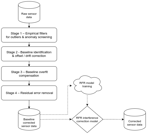
Figure 2Schematic of the sensor baseline correction model including interfaces with the downstream RFR interference correction model.
Table 1Filtering criteria used for the initial screening out of anomalous sensor data.
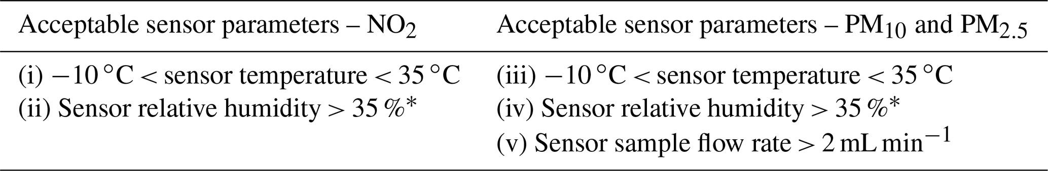
Filters (i)–(iv) were derived from local meteorological data. Filter (v) is a manufacturer recommendation. * There were ∼1400 15 min periods or 2.5 weeks (total) in 2020 when relative humidity was <35 %.
2.3.1 Stage 1 – empirical filters for removal of outliers and anomalies
The data-filtering criteria presented in Table 1 was developed to facilitate pragmatic screening of anomalous sensor data points. Their development was informed by a combination of local meteorological observations, data-logged by the reference monitoring station, and an analysis of typical sensor performance from the sensor. The acceptable sample flow rate criteria for the PM sensor was recommended by the manufacturer. When one or more parameters were detected outside the bands of acceptance shown (in Table 1), the sensor observation(s) were excluded from further analysis. Filters for NO2 and particles are presented in Table 1. Filters (i) and (iii) removed data points outside of precautionary estimates of the normal range of ambient temperature in Oxford, thereby excluding any anomalies arising from temperature-dependent sensor system corrections that may be performing out of range. Filters (ii) and (iv) performed a similar role for relative humidity. Filter (v) removed particles data during periods of low OPC sample flow rate. Application of these empirical filters rejected ∼1 % of the initialisation dataset.
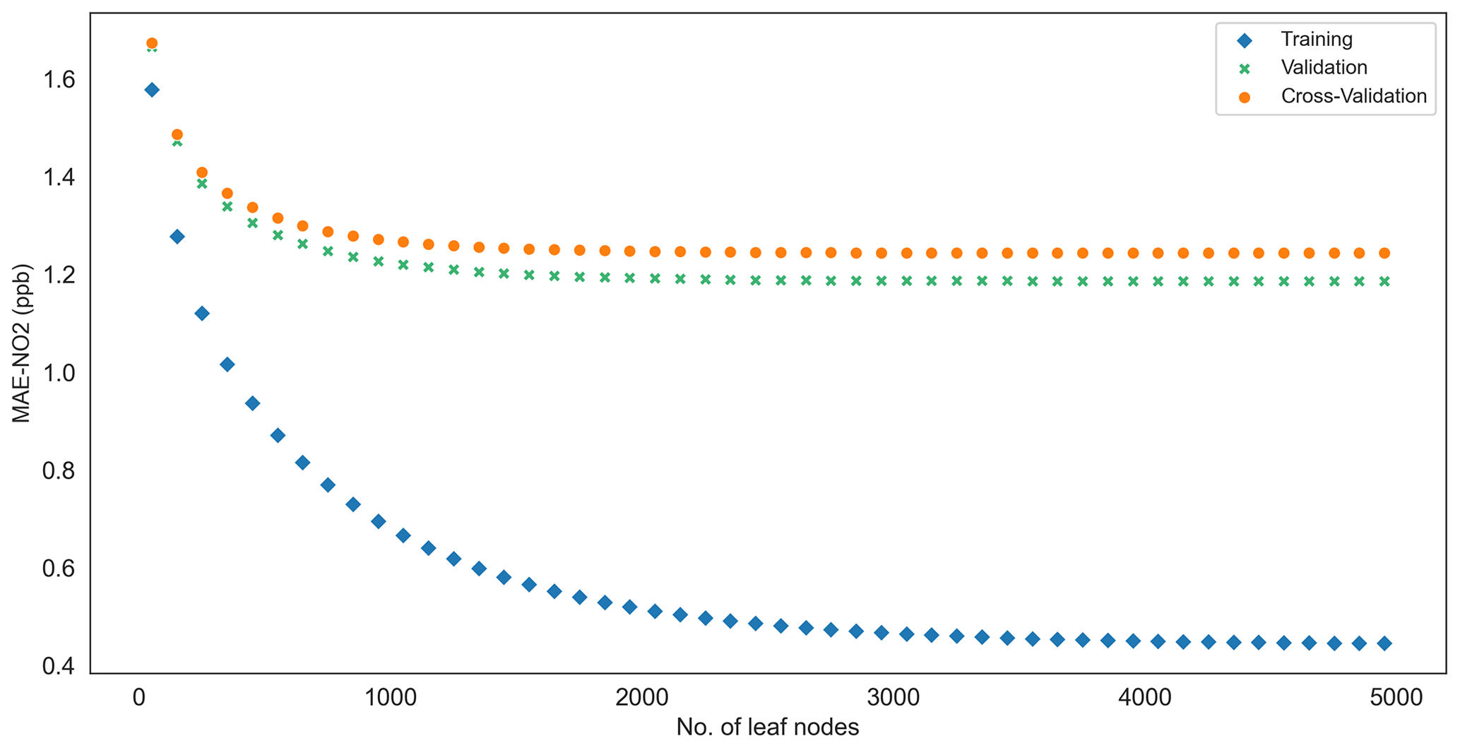
Figure 3NO2 RFR model performance returns with increasing model complexity (maximum number of leaf nodes included in training, validation and cross-validation datasets).
2.3.2 Stage 2 – baseline identification and offset/drift correction
Stage 2 implemented a statistical method developed in the analytical domain for baseline correction in chromatography and Raman spectroscopy. The method, adaptive iteratively reweighted penalised least squares (airPLS) (Zhang et al., 2010, 2011), combines least-squares regression smoothing, a penalty to control the amount of smoothing and a weighting function to constrain the baseline from following peaks in the sensor signal. Weightings are changed iteratively, after an initial best fit, with large weights applied where the newly iterated signal was below the previously fitted baseline and conversely small weights applied where the signal was above the fitted baseline.
Performance and flexibility were key factors in the selection of a preferred method for baseline correction. airPLS requires neither significant user intervention to perform satisfactorily nor prior information or supervision, e.g. peak detection. It is a fast, flexible technique and readily deployable in code (Zhang et al., 2011). In addition, airPLS offers important benefits as a controlled, systematic and reproducible approach to the handling of baseline offset in individual and networked sensors. No data losses occurred in stage 2 corrections.
2.3.3 Stage 3 – baseline overfit compensation
airPLS is highly efficient in correcting a baseline to zero, an artefact that derives from its intended application domain (chromatography) where a zero baseline is generally encouraged. Stage 3 applies a compensation method for the efficacy of the airPLS algorithm in correcting sensor baseline to zero, which in effect removes the urban, regional and rural background contributions from the sensor signal. The method scales the stage 2 outputs by the difference between the identified stage 2 baseline and that of the city scale background, the latter having been calculated using airPLS in this case using observations from the Oxford St Ebbe's urban-background AURN station. A compensation was calculated for each data point, i.e. at a 15 min time resolution. Taking the NO2 time series this compensation method resulted in an average uplift of +2.4 ppb. For PM10 and PM2.5 the uplift was +2.6 and +1.5 µg m−3 respectively. No data losses occurred during the stage 3 corrections.
2.3.4 Stage 4 – residual-error removal
The final stage of the sensor offset correction method accounts for the remaining residual anomalies that present as negative concentrations not accounted for in stages 1–3. The impact of this stage on the sample population was intended to be low and accounted for a further ∼3 % reduction in sample size. Approximately 6 months of continuous 15 min mean sensor data, paired with reference methods concentrations, was then used for RF training and validation activities.
2.4 Sensor interference correction with random forest regression modelling
The following sections present the configuration of the RF model and approach to model training. RF modelling was carried out in Python implemented using the scikit-learn open-source machine learning library (Pedregosa et al., 2011).
2.4.1 Feature engineering
Feature engineering describes the process of creating new training features (variables/parameters) that are more illustrative of the underlying problem being modelled. The aim of feature engineering is to affect better model training and performance. It is a common pre-processing step in RF modelling and many other regression and classification techniques (Breiman, 2001; Yu et al., 2011).
Feature engineering was constrained in scope and complexity by the need to deploy the model across a network of sensors. Hence, feature datasets must be readily available or replicable throughout the network of sensors. This operational constraint introduced a simplification of the known environmental interferences acting upon the Alphasense NO2-A43F electrochemical sensor. Spinelle et al. (2017b) reported evidence of cross sensitivities with NO2 and O3 on the (similar) Alphasense NO2-B43F electrochemical sensors. However, because O3 was only measured at half of the wider OxAria sensor network and is less commonly found within an air quality management setting in the UK, we chose to forego its inclusion as a training feature for the RF correction model. Although this may come with the penalty of reduced model training performance – Spinelle et al. (2017b) reported an O3-to-NO2 cross sensitivity of ∼6 % ppb−1 of NO2 – it comes with the benefit of a potentially broader real-world application domain, outside of a research setting.
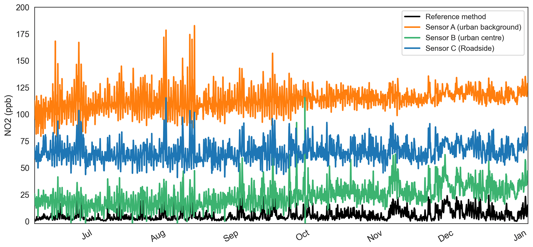
Figure 4A 3 h rolling mean raw low-cost sensor and reference method NO2 time series at three locations in Oxford for 2020.
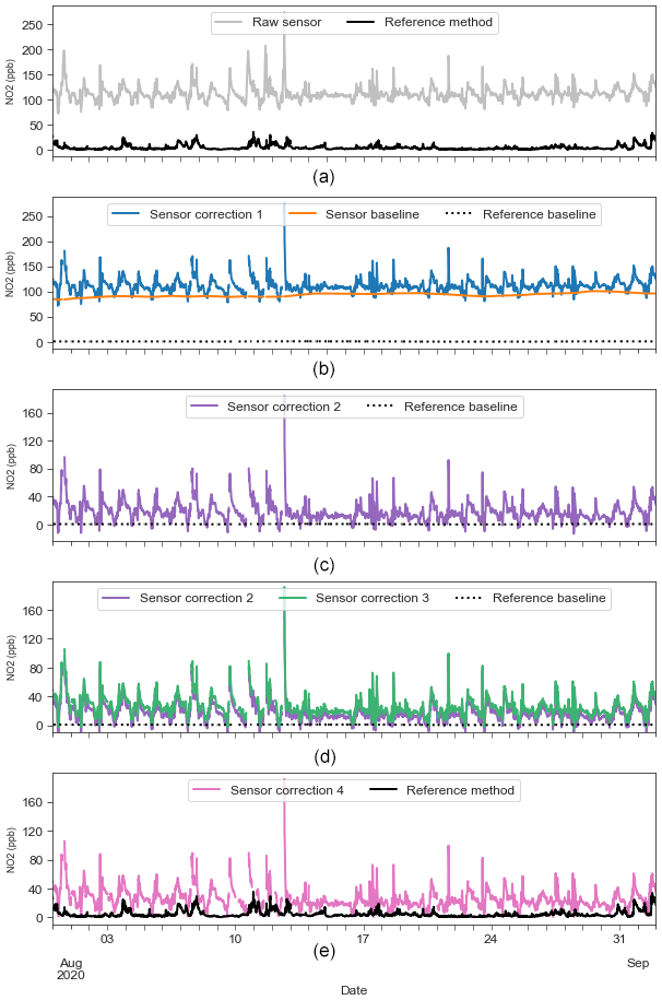
Figure 5Illustrative impacts of each stage in the sensor baseline offset correction model upon 15 min mean sensor observations at St Ebbe's for August 2020. (a) Raw sensor signal and reference method. (b) Correction 1 – application of empirical filters for anomaly and outlier removal. (c) Correction 2 – baseline offset correction. (d) Correction 3 – compensation for efficacy of baseline offset correction. (e) Correction 4 – removal of residuals. This figure presents the sensor offset correction model for illustrative purposes. Outputs from (e) are in turn parsed by the RF interference correction model to correct for transient effects of environmental parameters (not shown).
Table 2Model feature (variables) used in RF model training and prediction by the pollutant model. T: current time.
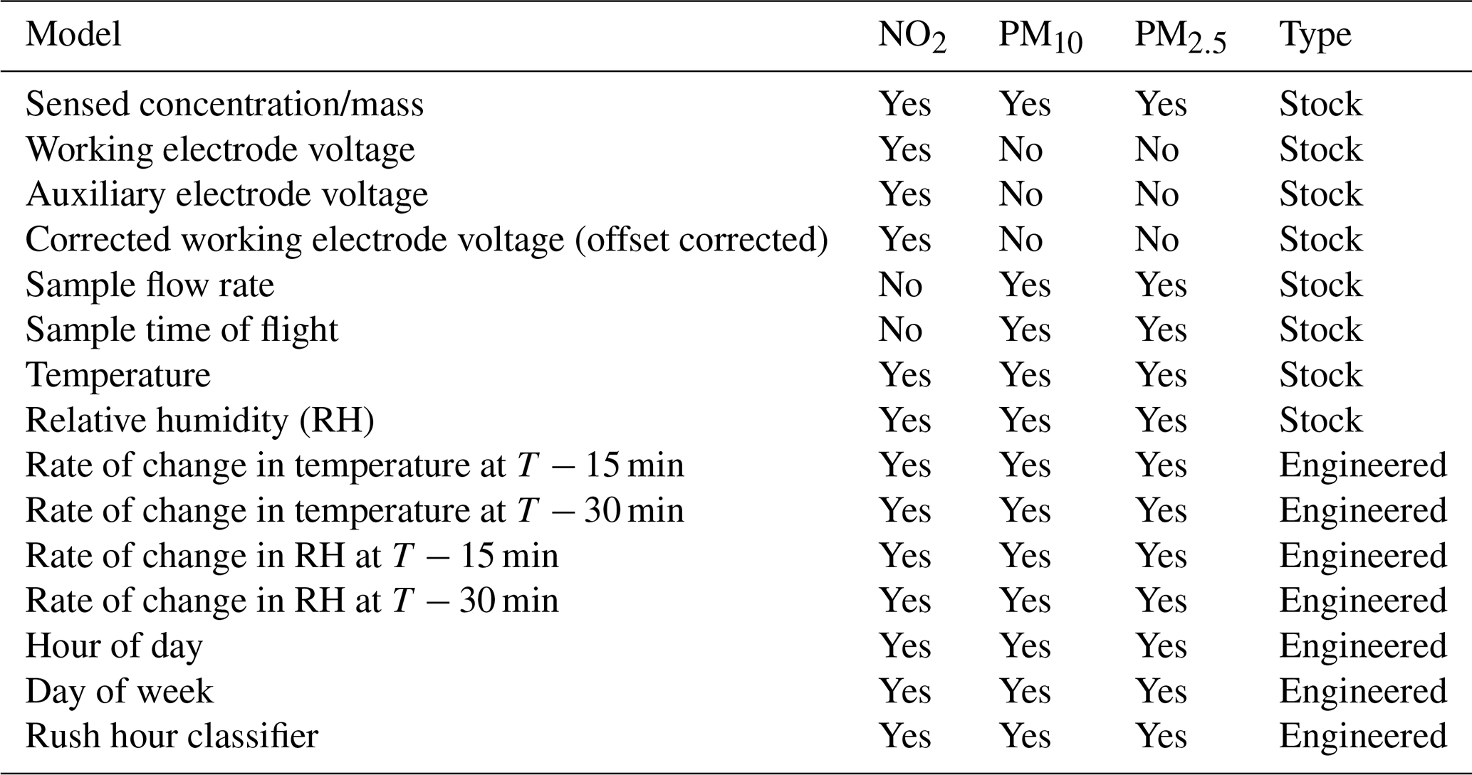
“Stock” indicates a feature based directly upon logged sensor observations. “Engineered” indicates a featured derived from re-analysis of one of more stock features.
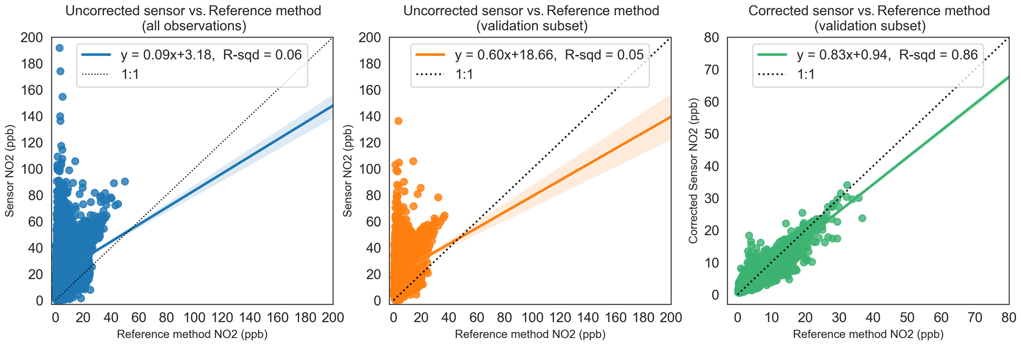
Figure 6Relationship between uncorrected sensor, RF-model-corrected sensor and reference method observations for NO2. The dotted line shows the unity slope. R-sqd: R2.
Table 2 presents the features used in model training of the pollutant specific correction model. The source of the training feature is presented in the “Type” column.
2.4.2 Random forest regression model training
RF model training was performed with co-located sensor and reference measurements acquired at the St Ebbe's AURN monitoring station over the period June to November 2020. After feature engineering (above), the core dataset was split into training and validation datasets using a 75 %-to-25 % split respectively. This “hold-out” validation method was combined with a k-fold cross-validation approach (Berrar, 2018) to estimate the performance of the model in terms of the mean absolute error (MAE) score (Buitinck et al., 2013; Pedregosa et al., 2011).
In many cases, RF models work reasonably well with the default values for the hyperparameters specified in the software packages (Probst et al., 2019). Even so, for standardisation across pollutant applications and computational efficiency we considered constraining the models using tree size metrics – number of trees, maximum number of leaf nodes and the minimum number of samples required to split an internal node.
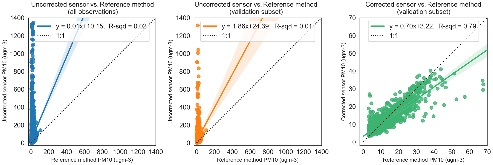
Figure 7Relationship between uncorrected sensor, RF-model-corrected sensor and reference method observations for PM10. The dotted line shows the unity slope. R-sqd: R2. ugm-3: µg m−3.

Figure 8Relationship between uncorrected sensor, RF-model-corrected sensor and reference method observations for PM2.5. The dotted line shows the unity slope. R-sqd: R2. ugm-3: µg m−3.
The maximum number of leaf nodes hyperparameter was established by way of a cross-validation sensitivity test on an array of 10 to 5000 nodes (node spacing set to 50). The cross-validation exercise fitted an RFR model to the input feature dataset and iterated over the array of nodes to predict the MAE. Cross-validation results for NO2 are presented in Fig. 3. These are illustrative of similar behaviours for PM10 and PM2.5. Figure 3 shows the MAE decreasing as a function of increasing maximum number of leaf nodes (model complexity). Cross-validation results similar to those presented in Fig. 3 were used to identify the optimum number of leaf nodes for each pollutant-specific model, the point on the x axis where increased model complexity delivers only a marginal improvement in the MAE for training, validation and cross-validation test samples. The process was repeated for the PM10 and PM2.5 models. Figure 3 also confirms some assumptions about RFR model training in general:
-
Gains in the MAE quickly drop-off with increasing feature numbers.
-
For RF model predictions which are based on an ensemble average of all trees, the MAE of predictions based on training data will tend towards but never reach zero.
-
k-fold cross-validation produced the most conservative estimates of model accuracy (highest MAE).
The maximum of 3500 of leaf nodes was established by this cross-validation process for the NO2 RFR model, whereas the same hyperparameter for both PM10 and PM2.5 models was set at 3000 nodes. The minimum number of samples allowed in a single partition was set to 2.
Table 3Summary of random forest hyperparameter settings used in model training.
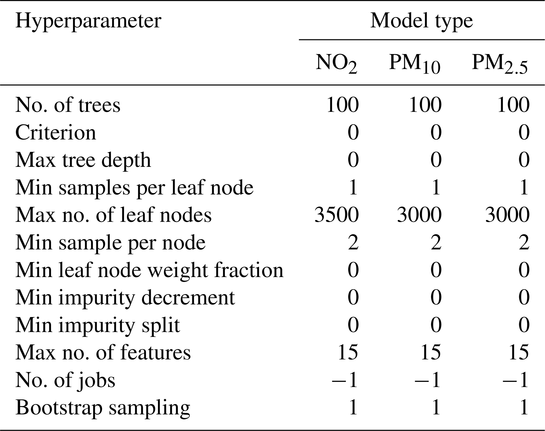
Having established the maximum number of leaf nodes for the three pollutant-specific models (NO2, PM10 and PM2.5), the number of trees was determined. The best practice on setting the optimum number of trees within RF is variable with advice ranging from between 64–128 (Oshiro et al., 2012). For this research, the incremental improvement in the MAE arising from between 100 and 500 trees was evaluated. Results did not show significant improvement in the model MAE over this range within the context of the typical ambient air quality concentrations expected. The number of trees used was set to 100 to minimise computational cost during training. Table 3 presents a summary of the hyperparameters used in the training of each random forest model. As a check on the hyperparameters presented in Table 3, the model's sensitivity to departures from these parameters was tested using the scikit-learn GridSearch function (Pedregosa et al., 2011). These tests showed that only small (<0.01 ppb) improvements in the MAE associated with the validation could be achieved by further tuning the hyperparameters shown in Table 3.
3.1 Uncorrected sensor data
Figure 4 presents the 3 h rolling mean of “raw” real-world NO2 observations from three OxAria low-cost electrochemical sensors and a reference method, i.e. sensor data outputs before any correction algorithms are applied. The rolling 3 h mean is presented to attenuate noise in the datasets for visualisation. Sensor A and the reference method are co-located at an urban-background location; sensor B is located at an urban centre location; and sensor C is at a roadside location. The sensor systems are identical and were calibrated at the same time by the manufacturer. Figure 4 shows a comparatively low signal-to-noise ratio in the sensor's observations when compared with the reference method and marked variability in the baseline(s) which confound interpretation of the pollutant levels. The severity of the variability in sensor baseline offset is further contextualised when sensor location is considered (as noted above). Sensor A being at the urban background is far from significant NO2 emissions sources, whereas sensors B (urban centre) and C (roadside) are comparatively close to major road transport emission sources. Despite their relative proximity to emission sources, the baseline for the urban-background sensor is ∼40 ppb higher than its urban-centre/roadside neighbours. Given that the sensors were calibrated to the same standard within a laboratory environment prior to deployment in the field, our assumption is that the sensor baselines have been influenced in some way after calibration, then stabilised as shown. In addition, frequent spikes in the sensor trace(s) can be observed which manifest as both short-lived, transient events of ∼10 s duration in the 100–500 ppb range and as longer-lived >60 s events, frequently in the 1000–2000 ppb range. This sort of sensor behaviour is linked to multiple environmental interferences of which temperature and relative humidity are amongst the most important (Spinelle et al., 2015). We anticipate that these sensor characteristics are replicated across the OxAria sensor network and indeed throughout similar sensor networks using electrochemical NO2 sensors and are therefore the focus of the sensor offset correction model described in the following sections.
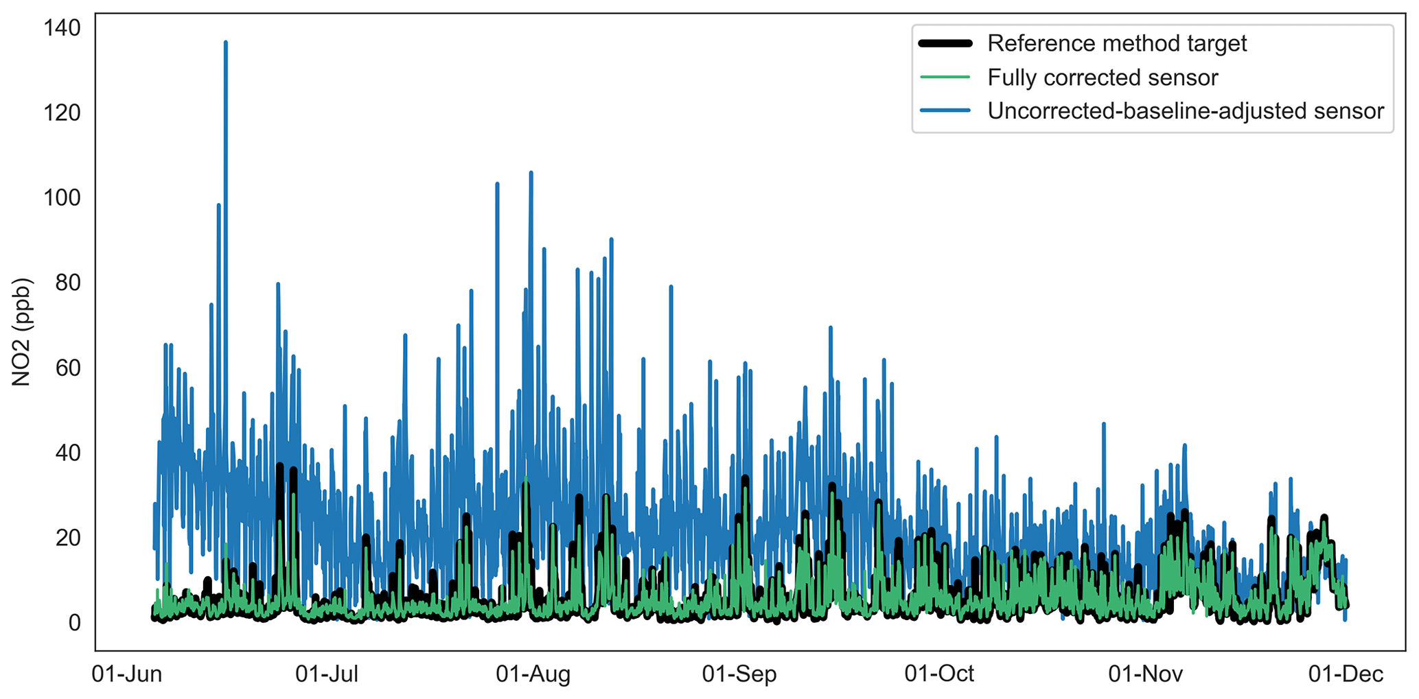
Figure 9Time series of uncorrected-baseline-adjusted sensor, fully corrected sensor and reference method observations for NO2 at Oxford St Ebbe's for 2020.
3.2 Sensor baseline offset correction results
Figure 5 presents the incremental outputs of each stage of the sensor baseline correction model described in Sect. 2.3. As an example, co-located NO2 sensor and reference method observations from St Ebbe's are presented for August 2020. This sensor and fragment of the 2020 time series were chosen as illustrative of the performance of the model on a sensor of a known offset (∼80 ppb) and the general effect of each stage in the correction process.
Commenting individually on each stage presented in Fig. 5, Fig. 5a indicates the presence of a clear offset in the NO2 sensor signal of ppb relative to the co-located reference method. Figure 5b presents the outcome of applying empirical filters to screen out anomalous sensor behaviours and data outliers. Noticeably for this location, the empirical filters have screened out observations around 10 August but left the >250 ppb spike in concentrations on 13 August in place. Figure 5c presents the removal of the sensor baseline using airPLS, and Fig. 5d shows compensation for its efficacy; the baselines of the part-corrected sensor time series and reference method baseline are recalculated (again using airPLS), and the sensor baseline is scaled by the difference in the two terms. The last step shown in Fig. 5e removes any residual negative errors not already captured.
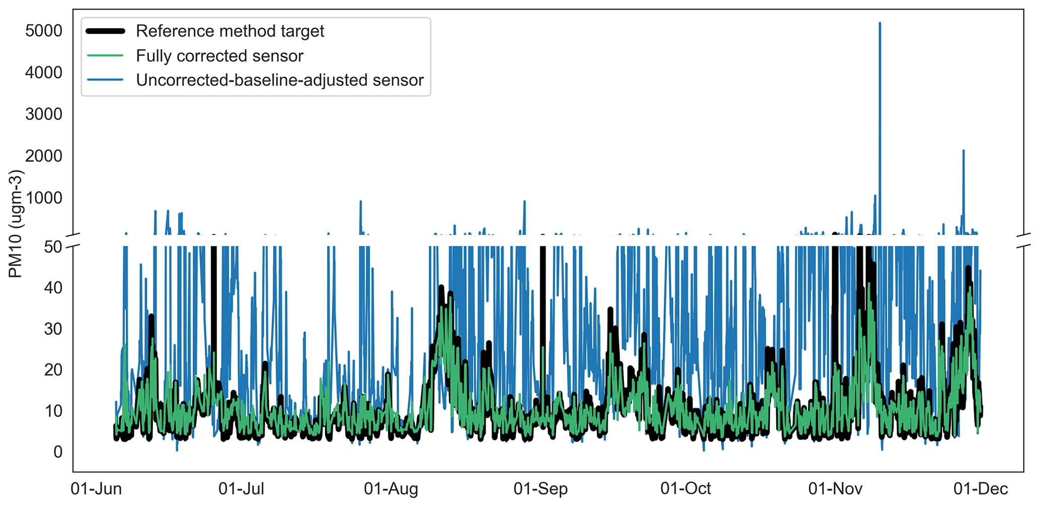
Figure 10Time series of uncorrected-baseline-adjusted sensor, fully corrected sensor and reference method observations for PM10 at Oxford St Ebbe's for 2020. ugm-3: µg m−3.
The data presented in Fig. 5c show the airPLS-based baseline correction model to be effective at standardising the variable baseline shown in the NO2, PM10 and PM2.5 sensor signals across the network. The method also maintains the fidelity of the dynamic range of the original sensor signal. Its effectiveness facilitates the training of generalised RF correction models. In terms of optimisations, the approach was relatively insensitive to changes in the configuration of the empirical filters applied in stage 1 corrections and the lambda value of the airPLS technique which controls the order of smoothing applied to the baseline estimate.
The overfitting of the part-corrected sensor baseline (to 0 ppb) introduced by the efficacy of the airPLS technique is compensated for by rescaling the sensor baseline to that of the city background. If this is an oversimplification of the experimental error handling, it is a reasonable trade-off given the volume of data involved and computational logistics involved overall.
The availability of a reliable and high-quality city background at a time resolution comparable to that of sensor observations, e.g. at most 15 min means, is essential for effectively screening transient anomalous sensor behaviours which skew sensor datasets significantly and mask important underlying data structures or anomalies. We also note that the reference method data-resolved to these time resolutions is difficult to obtain in the UK.
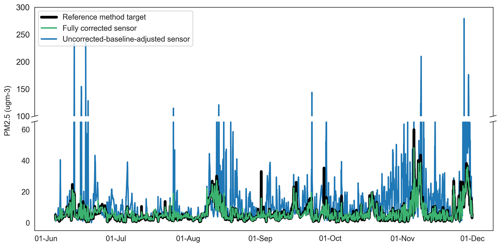
Figure 11Time series of uncorrected-baseline-adjusted sensor, fully corrected sensor and reference method observations for PM2.5 at Oxford St Ebbe's for 2020. ugm-3: µg m−3.
Table 4RFR correction model performance in terms of the MAE relative to reference method observations (validation data) for June to November 2020.
3.3 Random forest correction modelling results
3.3.1 Random forest regression model training
Outputs from the model training exercise are shown in Figs. 6–8 as a series of regression plots for the RFR models developed for NO2, PM10 and PM2.5. For each pollutant, three regression plots are presented to illustrate (i) the relationship between the baseline-corrected sensor observations and reference method (left), (ii) the same relationship constrained to the validation subset (middle), and (iii) the relationship between the fully corrected sensor observations (with both baseline correction and RFR interference corrections applied) and reference method. A simple ordinary least-squares (OLS) regression analysis is presented in each case to describe each relationship. All data shown are at a 15 min mean resolution.
The plots to the right of Figs. 6–8 show that the respective RF models are highly effective in predicting the target observations (reference method). In doing so, they demonstrate their capability to predict the combined interferences from a variety of environmental factors found in the data of the left and middle regression plots. The left and middle plots also show that training and validation datasets come from the same sample population (one having been randomly sampled from the other), providing a useful internal validation of model training to reflect variations in training features. Further checks on the models using unseen data from outside of the sample populations will better test likely performance of the models in the field.
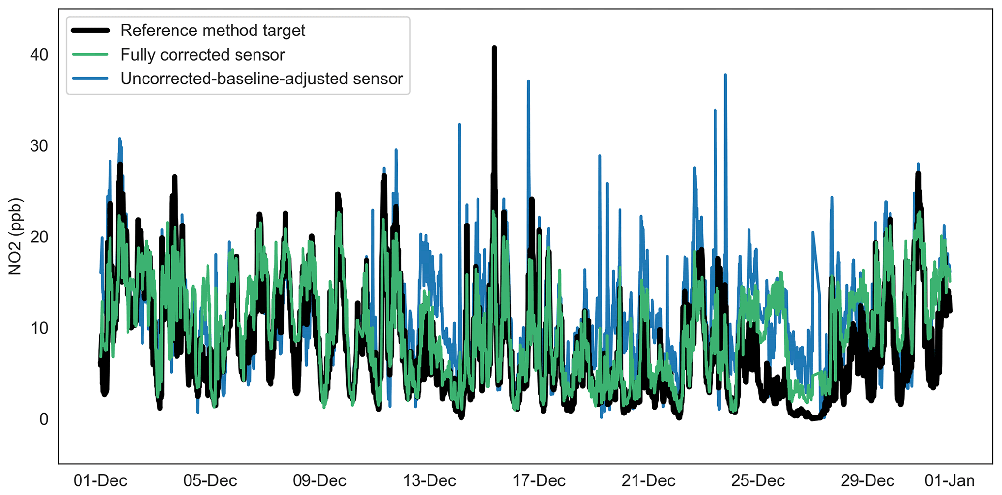
Figure 12Time series of uncorrected-baseline-adjusted sensor, fully corrected sensor and reference method observations for NO2 at Oxford St Ebbe's (unseen data) for December 2020.
Figures 6–8 show the dramatic impact of the RF model correction as demonstrated by the coefficients of variation in each of the three cases. The R2 value of the fully corrected sensor vs. reference method observations is a convenient evaluator for the ability of the models to capture the variability in the dependent datasets. Clearly, the PM2.5 model performs excellently in this respect with an R2 value of 0.91 and OLS slope and intercept terms approaching unity. The respective R2 value for both PM10 and NO2 RF models (0.79 and 0.86) also indicate good model performance. The values for R2 above are consistent with the out-of-bag scores achieved at training time (0.85, 0.79 and 0.91 for NO2, PM10, and PM2.5 respectively) which provide an additional check on model performance using data not explicitly used in the training. Even so, it is clear from Figs. 6 and 7 that the models struggled, on occasion, to accurately predict higher reference concentrations, and NO2 and PM10 predicted concentrations are generally more scattered compared with PM2.5. It is also noticeable that in all three cases the RF models are biased, tending to underpredict the reference concentration as demonstrated by the regression equation slope terms, and this is particularly noticeable in the >15 ppb concentration unit range.
Table 5RFR correction model performance in terms of the MAE relative to reference method observations (unseen data) for December 2020.

3.3.2 RF correction performance characteristics (hold-out validation set)
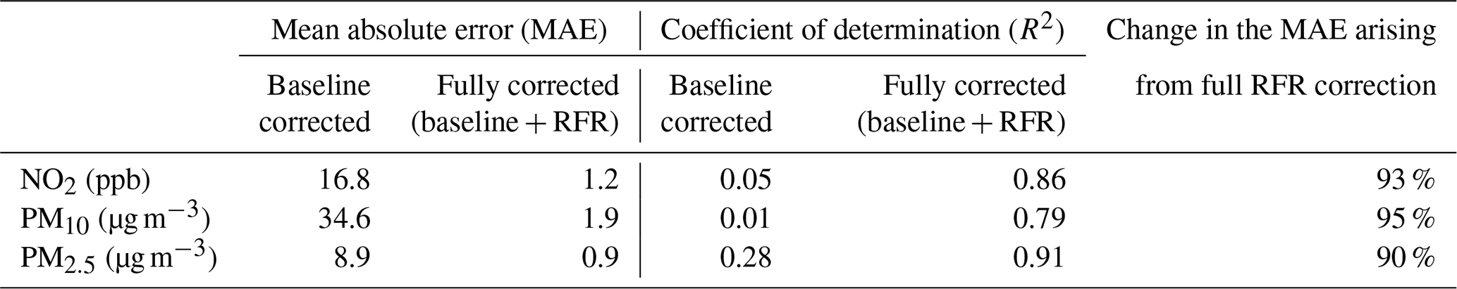
The performance of each component of the correction method upon 15 min mean data is presented in Table 4 in terms of the MAE delivered by correction outputs at each stage, relative to the reference method observations. Table 4 shows that the RFR correction adds significant value to the baseline correction, alone contributing to a further 90 %–95 % reduction in the MAE terms. In concentration units this equates to fully corrected NO2 sensor observations within approximately ±1.2 ppb of the reference observation. Similar comparisons for PM10 and PM2.5 indicate fully corrected concentrations within ±0.9 µg m−3 (PM10) and 1.9 µg m−3 (PM2.5) of the reference method. These compare favourably with results in the literature for all three pollutants.
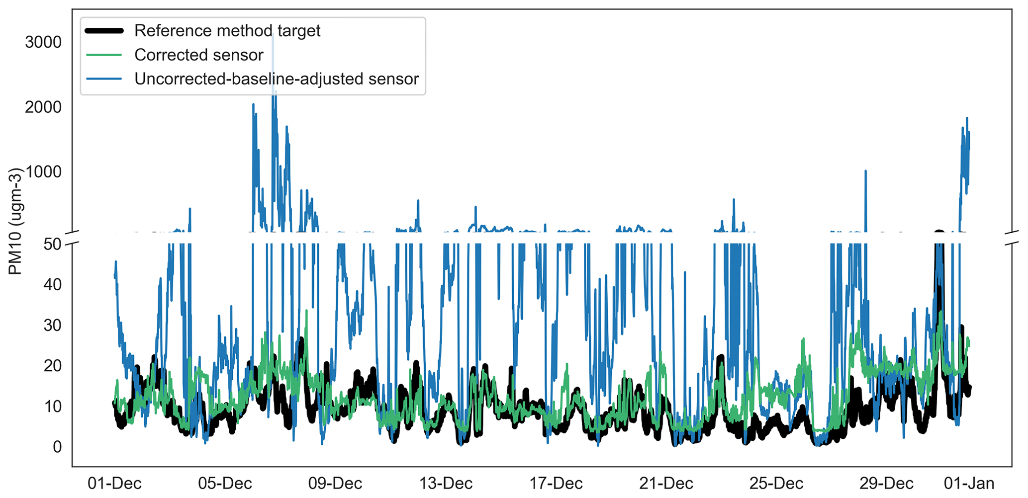
Figure 13Time series of uncorrected-baseline-adjusted sensor, fully corrected sensor and reference method observations for PM10 at Oxford St Ebbe's (unseen data) for December 2020. ugm-3: µg m−3.
The impact of corrections to this order of magnitude upon the sensor time series can be visualised in Figs. 9–11, which present 15 min mean uncorrected-baseline-adjusted sensor observations, fully corrected sensor observations and reference observations for NO2, PM10 and PM2.5. Figure 9 shows that for NO2 there is some visual evidence of the RFR model overcorrecting (relative to the reference method) during periods of peak concentration, particularly in mid to late June and August. Otherwise, the NO2 correction tracks that of the reference observations well.
3.3.3 RF correction model performance characteristics (unseen data)
Table 5 presents estimates of the correction model performance based on 15 min mean unseen data from December 2020, i.e. data used previously for neither model training nor validation. The data shown are, as expected, less favourable compared with the validation set, returning higher values for the MAE metric, but for the air quality context, these values are within 1.4 ppb (NO2) and 2.5 µg m−3 (PM10) and 1.8 µg m−3 (PM2.5) of the MAE returned by the model validation set (Tables 4 and 5).
In late November–December 2020 and latterly, continuing through the first quarter of 2021 (not shown), the sensor network observed episodes of high particle concentrations which coincided with a drop in ambient temperature (and dew point temperature) to the order of 10 ∘C. Neither reciprocal changes in relative humidity were observed, nor was there an obvious change in sensor sample flow rate. It is noteworthy also that similar conditions were not commonplace throughout the model training dataset (June to November 2020). The episode conditions observed by the sensor network were not replicated in the reference method dataset and are likely the main driver for the increase in the MAE for the particulate matter correction models shown in Table 5. Figures 13–14 show examples of the episodes in December 2020 for PM10 and PM2.5 respectively, including the absence of a reciprocal peak in the reference data and the performance of the model correction.
Despite these issues, and as demonstrated in Figs. 13–14, the RF models deliver substantial improvements on the raw dataset (not shown in Table 5) and baseline-adjusted data (shown). Improvements in the MAE attributable to the RF model in the range of 37 %–94 % are shown; these are equivalent to fully corrected observations within, on average, approximately ±2.6 ppb of the reference method for NO2, ±4.4 µg m−3 for PM10 and ±2.7 µg m−3 for PM2.5.
The decrease in model performance observed with the unseen dataset and the observations on ambient conditions and sensor operation (above) illustrate the need for long time series for model training, covering all environmental conditions to which the sensors will be exposed.
Table 6Expanded-uncertainty estimates for fully corrected sensor observations using the RFR validation dataset (the target values are the target expanded-uncertainty criteria recommended by European legislation).
∗ Expanded-uncertainty estimates with allowance to correct for a non-zero intercept and non-unitary slope in the linear regression relationship of the sensor to the reference method.
3.3.4 Corrected sensor performance vs. European air quality data quality objectives
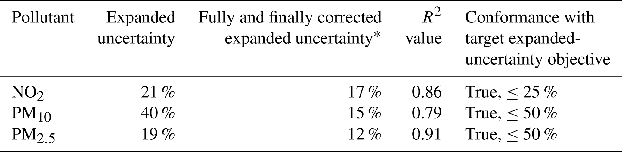
Tables 6 and 7 present expanded-uncertainty estimates for fully corrected sensor observations. These estimates were calculated using a spreadsheet tool (EC Working Group, 2020) to provide a further performance indicator on the adequacy of these data for air quality assessment applications. Table 6 presents expanded-uncertainty estimates associated with fully corrected sensor data from the validation dataset (data not used in the RFR model training) and shows that these data for all pollutants perform well against the target expanded-uncertainty criteria recommended by European legislation (expanded uncertainties of 21 %, 40 % and 19 % respectively for NO2, PM10 and PM2.5). Guidance on the calculation of expanded uncertainty (EC Working Group, 2010) also allows for the correction of slope and intercept terms in the relationship between the sensor and reference method. The result of this further correction is presented in Table 6 as the “full and final correction”. Expanded-uncertainty estimates for the validation set with full and final corrections applied were 17 %, 15 % and 12 % for NO2, PM10 and PM2.5 respectively. Highly respectable coefficients of determination between reference and fully and finally corrected sensor observations were also found in all cases as already shown in Figs. 6–8. However, because the validation set and model training datasets are closely coupled – the validation set being taken at random from the same sample population as that used for model training – expanded-uncertainty estimates based solely on these data should be interpreted with caution and may, depending on the application scenario of the correction model, present an overly optimistic estimate of real-world measurement uncertainty.
Table 7Expanded-uncertainty estimates for fully corrected sensor observations from an unseen dataset for December 2020 (the target values are the target expanded-uncertainty criteria recommended by European legislation).
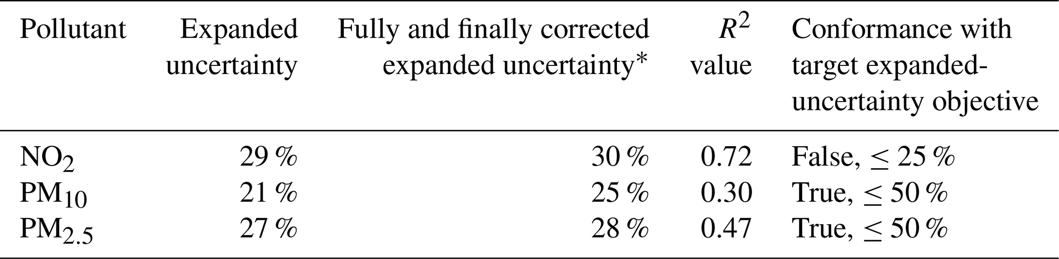
∗ Expanded-uncertainty estimates with allowance to correct for a non-zero intercept and non-unitary slope in the linear regression relationship of the sensor to the reference method.
Results from reciprocal calculations based on unseen data offer a more rigorous/precautionary test of expanded uncertainty, indicative of real-world applications. Table 7 presents these data for fully corrected sensor observations from December 2020. Table 7 shows the expanded-uncertainty estimates for fully corrected unseen sensor data of 29 %, 21 % and 27 % respectively for NO2, PM10 and PM2.5. Further corrections, for slope and intercept terms, had negligible change on these estimates (30 %, 25 % and 28 % expanded uncertainty respectively for NO2, PM10 and PM2.5). As expected, these data are more uncertain than the validation set; even so, performance is good relative to the target data quality objectives (DQOs). The fully and finally corrected datasets for PM10 and PM2.5 meet the expanded-uncertainty criteria recommended by European legislation. The expanded-uncertainty estimate for NO2 was within 5 % of the acceptance criteria.
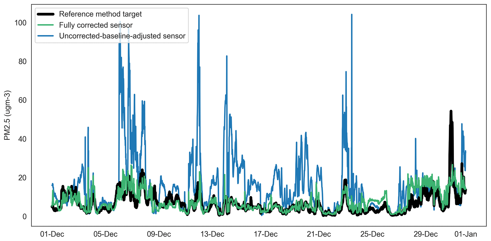
Figure 14Time series of uncorrected-baseline-adjusted sensor, fully corrected sensor and reference method observations for PM2.5 at Oxford St Ebbe's (unseen data) for December 2020. ugm-3: µg m−3.
This study has presented and demonstrated a simple and effective method for attenuating the confounding effects of sensor baseline variability and interferences from ambient environmental parameters upon low-cost electrochemical and optical particle counter sensor signals.
The methods presented in this paper have been tested at a high temporal resolution against high-quality, co-located reference method observations sourced from the UK's regulatory monitoring network (AURN). Using the MAE as an indicator of sensor error (relative to reference observations), the methods developed can reduce the error in NO2, PM10 and PM2.5 observations from the low-cost sensors tested by up to 88 %–95 % (based on model validation data not used in RF training). In the case of the low-cost NO2 sensor, corrections reduced the MAE of sensor observations to within ±1.2 ppb of the reference observation. Similarly, for PM10 and PM2.5, MAE estimates were within ±1.9 and ±0.9 µg m−3 respectively. The R2 value achieved for fully corrected NO2, PM10 and PM2.5 sensor observations were 0.86, 0.79 and 0.91 respectively.
Tests on how the methods generalised to unseen conditions have shown that the RFR correction models trained on data from June to November 2020 are tolerant of a wide range of competing environmental interferences. Tests based on data from December 2020, unseen by the RF model in training, delivered MAE estimates for fully corrected low-cost NO2, PM10 and PM2.5 sensors of 2.6 ppb, 4.4 and 2.7 µg m−3 respectively. Despite this observed (and expected) drop in performance, the MAE values in corrections to unseen datasets were within 1.4 ppb (NO2) and 2.5 µg m−3 (PM10) and 1.8 µg m−3 (PM2.5) of those returned by the model validation set.
Given these indicators for the level of improved uncertainty that can be achievable with the methods presented, we propose that data from reputable, high-quality sensors may now have a meaningful role in the air quality assessment toolkit. Indeed, using the methods presented, sensor data may deliver data quality of at least comparable levels to that displayed by passive sampler methods (for NO2), with the benefit of higher temporal resolution.
To substantiate potential future applications, this paper has presented data demonstrating that the RF-based methods are capable of delivering fully corrected low-cost sensor data that meet the general requirements for “indicative measurements” as set out by the European Ambient Air Quality Directive. In doing so, we have used methods prescribed by the European Commission Working Group on Guidance for the Demonstration of Equivalence to calculate expanded-uncertainty estimates for fully corrected sensor observations. For tests based on validation and unseen datasets, the expanded uncertainty of fully corrected sensor data was within the requirements set by the European Ambient Air Quality Directive for indicative monitoring (within ±25 % of the reference observation for NO2, ±50 % for particles) for PM10 and PM2.5. Estimates for NO2 were outside of the acceptance criteria by ∼5 %. Fully corrected expanded-uncertainty estimates for PM10 and PM2.5 were within or proximal to the equivalence thresholds (±25 %) established by the European Commission Working Group on Guidance for the Demonstration of Equivalence. In tests using unseen data, the most stringent test available to the study, the expanded-uncertainty estimates for RFR-model-corrected observations for NO2, PM10 and PM2.5 were 30 %, 25 % and 28 % respectively.
Demonstrating conformance with these regulatory thresholds in a traceable way is a significant milestone, not only for the potential to unlock applications as “supplementary assessment” methods for compliance assessments but also within the context of the stringency of the acceptance criteria and the rigour of the expanded-uncertainty calculation method set out by the working group.
We anticipate application of the model in other local contexts will require re-training and validation of the RF model for local conditions, an important focus for future research. As such, the techniques developed are presented as a working method to be adapted for other applications rather than a definitive model for wider generalisations. We also note that scaling of the method to applications across a sensor network is likely to be limited by the diversity of the RF training datasets and the quality of the city scale background (both spatial and scalar representativeness). However, this work has demonstrated capabilities for applications to monitoring across a small city, with clear potential benefits for supporting air quality management.
Code arising from this study is being prepared for deposit in the UK Natural Environment Research Council (NERC) Centre for Environmental Data Analysis (CEDA) Archive at https://www.ceda.ac.uk/services/ceda-archive/ (CEDA Archive, 2022). Prior to deposit in CEDA, data are available from the corresponding authors upon request.
Reference measurement datasets at 15 min resolution were sourced from Ricardo Energy & Environment, Harwell, UK (Brian Stacey, personal communication, throughout 2020–2021). Reference measurement datasets at 1 h resolution were sourced from https://uk-air.defra.gov.uk/data/ (Defra, 2022). Sensor datasets arising from this study are being prepared for deposit in the UK Natural Environment Research Council (NERC) Centre for Environmental Data Analysis (CEDA) Archive at https://www.ceda.ac.uk/services/ceda-archive/ (CEDA Archive, 2022). Prior to deposit in CEDA, data are available from the corresponding authors upon request.
FL, NP, SB and TB conceived the study. TB and FL corralled the data. TB and NP performed data analysis. BS supplied reference observations at the required resolutions and finessed expanded-uncertainty estimates in accordance with the guidance. TB drafted the paper. All co-authors contributed to reviewing and editing the paper.
At least one of the (co-)authors is a member of the editorial board of Atmospheric Measurement Techniques. The peer-review process was guided by an independent editor, and the authors also have no other competing interests to declare.
Publisher’s note: Copernicus Publications remains neutral with regard to jurisdictional claims in published maps and institutional affiliations.
The authors would like to extend thanks and gratitude to the chair of the project steering committee, the late Martin Williams, for his guidance and encouragement over the years. The authors would also like to thank the study steering group for their technical contributions and administrative support and Ricardo Energy & Environment for facilitating data acquisition. Oxford City Council and Oxfordshire County Council are both thanked for advice and support.
This research was funded by the Natural Environment Research Council (grant no. NE/V010360/1). Its forerunning pilot project was funded by the National Institute for Health and Care Research (NIHR130095; NIHR Public Health Research). The views expressed are those of the author(s) and not necessarily those of the NIHR or the Department of Health and Social Care. This publication arises in part from research funded by Research England's Strategic Priorities Fund (SPF) quality related (QR) allocation.
This paper was edited by Pierre Herckes and reviewed by two anonymous referees.
Alphasense Ltd.: NO2-A43F Nitrogen Dioxide Sensor 4-Electrode Technical Specification, https://www.alphasense.com/wp-content/uploads/2019/09/NO2-A43F.pdf (last access: 19 May 2021), 2019a.
Alphasense Ltd.: OPC-N3 Particle Monitor Technical Specification, https://www.alphasense.com/wp-content/uploads/2019/03/OPC-N3.pdf (last access: 19 May 2021), 2019b.
Berrar, D.: Cross-validation, in Encyclopaedia of Bioinformatics and Computational Biology: ABC of Bioinformatics, Elsevier, 3, 542–545, 2018.
Bigi, A., Mueller, M., Grange, S. K., Ghermandi, G., and Hueglin, C.: Performance of NO, NO2 low cost sensors and three calibration approaches within a real world application, Atmos. Meas. Tech., 11, 3717–3735, https://doi.org/10.5194/amt-11-3717-2018, 2018.
Breiman, L.: Bagging predictors, Mach. Learn., 24, 123–140, https://doi.org/10.1023/A:1018054314350, 1996.
Breiman, L.: Random forests, Mach. Learn., 45, 5–32, https://doi.org/10.1023/A:1010933404324, 2001.
Castell, N., Dauge, F. R., Schneider, P., Vogt, M., Lerner, U., Fishbain, B., Broday, D., and Bartonova, A.: Can commercial low-cost sensor platforms contribute to air quality monitoring and exposure estimates?, Environ. Int., 99, 293–302, https://doi.org/10.1016/j.envint.2016.12.007, 2017.
CEDA: CEDA Archive, STFC, UK, CEDA [code, data set], https://www.ceda.ac.uk/services/ceda-archive/, last access: 24 May 2022.
Clements, A. L., Reece, S., Conner, T., and Williams, R.: Observed data quality concerns involving low-cost air sensors, Atmos. Environ., 3, 100034, https://doi.org/10.1016/j.aeaoa.2019.100034, 2019.
Crilley, L. R., Shaw, M., Pound, R., Kramer, L. J., Price, R., Young, S., Lewis, A. C., and Pope, F. D.: Evaluation of a low-cost optical particle counter (Alphasense OPC-N2) for ambient air monitoring, Atmos. Meas. Tech., 11, 709–720, https://doi.org/10.5194/amt-11-709-2018, 2018.
Crilley, L. R., Singh, A., Kramer, L. J., Shaw, M. D., Alam, M. S., Apte, J. S., Bloss, W. J., Hildebrandt Ruiz, L., Fu, P., Fu, W., Gani, S., Gatari, M., Ilyinskaya, E., Lewis, A. C., Ng'ang'a, D., Sun, Y., Whitty, R. C. W., Yue, S., Young, S., and Pope, F. D.: Effect of aerosol composition on the performance of low-cost optical particle counter correction factors, Atmos. Meas. Tech., 13, 1181–1193, https://doi.org/10.5194/amt-13-1181-2020, 2020.
Cross, E. S., Williams, L. R., Lewis, D. K., Magoon, G. R., Onasch, T. B., Kaminsky, M. L., Worsnop, D. R., and Jayne, J. T.: Use of electrochemical sensors for measurement of air pollution: correcting interference response and validating measurements, Atmos. Meas. Tech., 10, 3575–3588, https://doi.org/10.5194/amt-10-3575-2017, 2017.
Defra: Quality Assurance and Quality Control (QA/QC) Procedures for UK Air Quality Monitoring under 2008/50/EC and 2004/107/EC, https://uk-air.defra.gov.uk/assets/documents/reports/cat09/1902040953_All_Networks_QAQC_Document_2012__Issue2.pdf (last access: 5 May 2021), 2013.
Defra: Clean Air Strategy 2019, https://www.gov.uk/government/publications/clean-air-strategy-2019 (last access: 24 May 2022), 2019.
Defra: Site Information for Oxford St Ebbes(UKA00518) – Defra, UK, https://uk-air.defra.gov.uk/networks/site-info?uka_id=UKA00518&provider=, last access: 21 April 2021.
Defra: UK Air Information Resource – Defra, UK [data set], https://uk-air.defra.gov.uk/data, last access: 24 May 2022.
Defra and DfT: UK plan for tackling roadside nitrogen dioxide concentrations: An overview, https://www.gov.uk/government/publications/air-quality-plan-for-nitrogen-dioxide-no2-in-uk-2017 (last access: 24 May 2022), 2017.
EC Working Group: Guide to the demonstration of equivalence of ambient air monitoring methods Report by an EC Working Group on Guidance for the Demonstration of Equivalence, https://ec.europa.eu/environment/air/quality/legislation/pdf/equivalence.pdf (last access: 24 May 2022), 2010.
EC Working Group: Equivalence Spreadsheet Tool on the Demonstration of Equivalence, Version Control, Version 3.1, 02/07/20, https://ec.europa.eu/environment/air/quality/legislation/pdf/EquivalenceTool%20V3.1%20020720.xlsx (last access: 5 May 2021), 2020.
Esposito, E., De Vito, S., Salvato, M., Bright, V., Jones, R. L., and Popoola, O.: Dynamic neural network architectures for on field stochastic calibration of indicative low-cost air quality sensing systems, Sensor. Actuat. B-Chem., 231, 701–713, https://doi.org/10.1016/j.snb.2016.03.038, 2016.
Hasenfratz, D., Saukh, O., and Thiele, L.: On-the-Fly Calibration of Low-Cost Gas Sensors, in Wireless Sensor Networks, edited by: Picco, P. G. and Heinzelman, W., Springer Berlin Heidelberg, Berlin, Heidelberg, 228–244, 2012.
Hastie, T., Tibshirani, R., and Friedman, J.: The Elements of Statistical Learning, https://doi.org/10.1007/978-0-387-84858-7, 2009.
Karagulian, F., Barbiere, M., Kotsev, A., Spinelle, L., Gerboles, M., Lagler, F., Redon, N., Crunaire, S., and Borowiak, A.: Review of the performance of low-cost sensors for air quality monitoring, Atmosphere, 10, 506, https://doi.org/10.3390/atmos10090506, 2019.
Kelly, F. P.: Associations of long-term average concentrations of nitrogen dioxide with motality, COMEAP Report, https://assets.publishing.service.gov.uk/government/uploads/system/uploads/attachment_data/file/734799/COMEAP_NO2_Report.pdf (last access: 24 May 2022), 2018.
Leach, F. C. P., Peckham, M. S., and Hammond, M. J.: Identifying NOx Hotspots in Transient Urban Driving of Two Diesel Buses and a Diesel Car, Atmosphere, 11, 355, https://doi.org/10.3390/atmos11040355, 2020.
Lim, C. C., Kim, H., Vilcassim, M. J. R., Thurston, G. D., Gordon, T., Chen, L. C., Lee, K., Heimbinder, M., and Kim, S. Y.: Mapping urban air quality using mobile sampling with low-cost sensors and machine learning in Seoul, South Korea, Environ. Int., 131, 105022, https://doi.org/10.1016/J.ENVINT.2019.105022, 2019.
Morawska, L., Thai, P. K., Liu, X., Asumadu-Sakyi, A., Ayoko, G., Bartonova, A., Bedini, A., Chai, F., Christensen, B., Dunbabin, M., Gao, J., Hagler, G. S. W., Jayaratne, R., Kumar, P., Lau, A. K. H., Louie, P. K. K., Mazaheri, M., Ning, Z., Motta, N., Mullins, B., Rahman, M. M., Ristovski, Z., Shafiei, M., Tjondronegoro, D., Westerdahl, D., and Williams, R.: Applications of low-cost sensing technologies for air quality monitoring and exposure assessment: How far have they gone?, Environ. Int., 116, 286–299, https://doi.org/10.1016/j.envint.2018.04.018, 2018.
National Institute for Health Research: NIHR Funding and Awards Search Website, https://fundingawards.nihr.ac.uk/award/NIHR130095 (last access: 24 May 2022), 2020.
Oshiro, T. M., Perez, P. S., and Baranauskas, J. A.: How Many Trees in a Random Forest?, in: Machine Learning and Data Mining in Pattern Recognition, edited by: Perner, P., MLDM 2012, Lecture Notes in Computer Science, Vol. 7376, Springer, Berlin, Heidelberg, https://doi.org/10.1007/978-3-642-31537-4_13, 2012.
Probst, P., Wright, M., and Boulesteix, A.-L.: Hyperparameters and Tuning Strategies for Random Forest, https://wires.onlinelibrary.wiley.com/doi/10.1002/widm.1301 (last access: 24 May 2022), 2019.
Public Health England: Health matters: air pollution – GOV. UK, UK Gov., November, https://www.gov.uk/government/publications/health-matters-air-pollution/health-matters-air-pollution (last access: 24 May 2022), 2018.
Schneider, P., Castell, N., Vogt, M., Dauge, F. R., Lahoz, W. A., and Bartonova, A.: Mapping urban air quality in near real-time using observations from low-cost sensors and model information, Environ. Int., 106, 234–247, https://doi.org/10.1016/j.envint.2017.05.005, 2017.
Spinelle, L., Gerboles, M., and Aleixandre, M.: Performance evaluation of amperometric sensors for the monitoring of O3 and NO2 in ambient air at ppb level, Procedia Eng., 120, 480–483, https://doi.org/10.1016/j.proeng.2015.08.676, 2015.
Spinelle, L., Gerboles, M., Villani, M. G., Aleixandre, M., and Bonavitacola, F.: Field calibration of a cluster of low-cost commercially available sensors for air quality monitoring. Part B: NO, CO and CO2, Sensor. Actuat. B-Chem., 238, 706–715, https://doi.org/10.1016/j.snb.2016.07.036, 2017a.
Spinelle, L., Gerboles, M., Kotsev, A., and Signorini, M.: Evaluation of low-cost sensors for air pollution monitoring: Effect of gaseous interfering compounds and meteorological conditions, JRC Technical Report, https://op.europa.eu/en/publication-detail/-/publication/23e1a2c7-3c41-11e7-a08e-01aa75ed71a1 (last access: 24 May 2022), 2017b.
De Vito, S., Piga, M., Martinotto, L., and Di Francia, G.: CO, NO2 and NOx urban pollution monitoring with on-field calibrated electronic nose by automatic bayesian regularization, ensor. Actuat. B-Chem., 143, 182–191, https://doi.org/10.1016/j.snb.2009.08.041, 2009.
Wang, S., Ma, Y., Wang, Z., Wang, L., Chi, X., Ding, A., Yao, M., Li, Y., Li, Q., Wu, M., Zhang, L., Xiao, Y., and Zhang, Y.: Mobile monitoring of urban air quality at high spatial resolution by low-cost sensors: impacts of COVID-19 pandemic lockdown, Atmos. Chem. Phys., 21, 7199–7215, https://doi.org/10.5194/acp-21-7199-2021, 2021.
Woodall, G., Hoover, M., Williams, R., Benedict, K., Harper, M., Soo, J.-C., Jarabek, A., Stewart, M., Brown, J., Hulla, J., Caudill, M., Clements, A., Kaufman, A., Parker, A., Keating, M., Balshaw, D., Garrahan, K., Burton, L., Batka, S., Limaye, V., Hakkinen, P., and Thompson, B.: Interpreting Mobile and Handheld Air Sensor Readings in Relation to Air Quality Standards and Health Effect Reference Values: Tackling the Challenges, Atmosphere, 8, 182, https://doi.org/10.3390/atmos8100182, 2017.
Yu, H., Lo, H., Hsieh, H., Lou, J., Mckenzie, T. G., Chou, J., Chung, P., Ho, C., Chang, C., Weng, J., Yan, E., Chang, C., Kuo, T., Chang, P. T., Po, C., Wang, C., Huang, Y., Ruan, Y., Lin, Y., Lin, S., Lin, H., and Lin, C.: Feature engineering and classifier ensemble for KDD Cup 2010, JMLR Work, Conf. Proc., http://citeseerx.ist.psu.edu/viewdoc/summary?doi=10.1.1.367.249 (last access: 4 May 2021), 2011.
Zhang, Z. M., Chen, S., and Liang, Y. Z.: Baseline correction using adaptive iteratively reweighted penalized least squares, Analyst, 135, 1138–1146, https://doi.org/10.1039/b922045c, 2010.
Zhang, Z. M., Chen, S., and Liang, Y. Z.: Google Code Archive – Long-term storage for Google Code Project Hosting, https://code.google.com/archive/p/airpls/ (last access: 5 May 2021), 2011.
Zimmerman, N., Presto, A. A., Kumar, S. P. N., Gu, J., Hauryliuk, A., Robinson, E. S., Robinson, A. L., and R. Subramanian: A machine learning calibration model using random forests to improve sensor performance for lower-cost air quality monitoring, Atmos. Meas. Tech., 11, 291–313, https://doi.org/10.5194/amt-11-291-2018, 2018.