Ch3MS-RF: a random forest model for chemical characterization and improved quantification of unidentified atmospheric organics detected by chromatography–mass spectrometry techniques

The chemical composition of ambient organic aerosols plays a critical role in driving their climate and health-relevant properties and holds important clues to the sources and formation mechanisms of secondary aerosol material. In most ambient atmospheric environments, this composition remains incompletely characterized, with the number of identifiable species consistently outnumbered by those that have no mass spectral matches in the literature or the National Institute of Standards and Technology/National Institutes of Health/Environmental Protection Agency (NIST/NIH/EPA) mass spectral databases, making them nearly impossible to definitively identify. This creates significant challenges in utilizing the full analytical capabilities of techniques which separate and generate spectra for complex environmental samples. In this work, we develop the use of machine learning techniques to quantify and characterize novel, or unidentifiable, organic material. This work introduces Ch3MS-RF (Chemical Characterization by Chromatography–Mass Spectrometry Random Forest Modeling), an open-source, R-based software tool, for efficient machine-learning-enabled characterization of compounds separated in chromatography–mass spectrometry applications but not identifiable by comparison to mass spectral databases. A random forest model is trained and tested on a known 130 component representative external standard to predict the response factors of novel environmental organics based on position in volatility–polarity space and mass spectrum, enabling the reproducible, efficient, and optimized quantification of novel environmental species. Quantification accuracy on a reserved 20 % test set randomly split from the external standard compound list indicates that random forest modeling significantly outperforms the commonly used methods in both precision and accuracy, with a median response factor percent error of −2 %, for modeled response factors, compared to > 15 %, for typically used proxy assignment-based methods. Chemical properties modeling, evaluated on the same reserved 20 % test set and an extrapolation set of species identified in ambient organic aerosol samples collected in the Amazon rainforest, also demonstrate robust performance. Extrapolation set property prediction mean absolute errors for carbon number, oxygen to carbon ratio (O : C), average carbon oxidation state ($\stackrel{\mathrm{‾}}{{\mathrm{OS}}_{\mathrm{c}}}$), and vapor pressure are 1.8, 0.15, 0.25, and 1.0 (log(atm)), respectively. Extrapolation set out-of-sample R² for all properties modeled are above 0.75, with the exception of vapor pressure. While predictive performance for vapor pressure is less robust compared to the other chemical properties modeled, random-forest-based modeling was significantly more accurate than other commonly used methods of vapor pressure prediction, decreasing the mean vapor pressure prediction error to 0.24 (log(atm)) from 0.55 (log(atm)) (chromatography-based vapor pressure prediction) and 1.2 (log(atm)) (chemical formula-based vapor pressure prediction). The random forest model significantly advances an untargeted analysis of the full scope of chemical speciation yielded by two-dimensional gas chromatography (GCxGC-MS) techniques and can be applied to gas chromatography coupled with electron ionization mass spectrometry (GC-MS) as well. It enables the accurate estimation of key chemical properties commonly utilized in the atmospheric chemistry community, which may be used to more efficiently identify important tracers for further individual analysis and to characterize compound populations uniquely formed under specific ambient conditions.

1 Introduction

Organic aerosols play a critical role in global radiative forcing and regional aerosol-attributable public health concerns, making up a significant (20 %–90 %) fraction of fine particulate matter around the globe (Jimenez et al., 2009). This organic material is highly complex in terms of chemical composition and is constantly changing; Goldstein and Galbally (2007) estimate the number of gas- and aerosol-phase atmospheric organic constituents to lie in the millions, while Ditto et al. (2018) report a molecular-level variability of 60 %–80 % between consecutive samples collected at fixed sites for samples comprised of high thousands of resolvable species. While there has been significant progress towards achieving mass closure of atmospheric reactive carbon using an ensemble of both bulk and speciated measurement techniques over the past 2 decades, speciated and isomer identified mass closure remains challenging (Heald et al., 2010; Hunter et al., 2017; Isaacman-Vanwertz et al., 2018). Using a comprehensive review of the challenges and utility of different levels of molecular identification, Nozière et al. (2015) compare the utility of many types of incomplete identification of atmospheric organic compounds, but define that “An organic compound is fully identified only if its molecular structure is entirely known, including its isomeric and spatial (stereo) configuration.” Important chemical information can be gleaned from formula-based identifications and bulk characterization, but isomer-specific identifications provide critical atmospheric chemistry-relevant insights. As described in Isaacman-Vanwertz and Aumont (2021), different isomers of the same chemical formula vary over orders of magnitude in volatility and Henry's constant, and by a factor of 2 in reactivity with the hydroxyl radical, which are all critical properties for the characterization of aerosol formation and properties. Isomer-specific identification also plays a crucial role in elucidation of important chemical reaction mechanisms.

Gas chromatography coupled with electron ionization mass spectrometry (GC-MS) is a commonly utilized technique for isomer-specific speciation of atmospheric constituents. Observed ambient species may be matched to authentic standards or mass spectral database entries by both the retention index (chromatographic elution time relative to that of a series of alkanes) and mass spectrum. A methodologically similar technique, two-dimensional gas chromatography (GCxGC-MS), achieves advanced separation by passing compounds through multiple GC columns configured for different chemical properties, which increases the scope of isomer-specific identification by separating species that would co-elute in single-dimension GC-MS applications (Goldstein et al., 2008; Worton et al., 2011, 2017). However, a significant challenge of fully utilizing the data from these techniques is the novelty and diversity of the atmospheric constituents; most observed organic species have never been synthesized and are not in any mass spectral library and are therefore not directly identifiable from GC-MS or GCxGC-MS techniques. Although the sizes of mass spectral libraries are rapidly increasing, with ∼ 30 000 new compounds added to the National Institute of Standards and Technology/National Institutes of Health/Environmental Protection Agency (NIST/NIH/EPA) mass spectral database between the 2011 and 2014 versions (bringing the number of compounds catalogued in NIST14 EI library to ∼ 250 000), the numbers of identifiable constituents in typical atmospheric samples remain low (Vinaixa et al., 2016). As described in Hamilton et al. (2004), in an urban aerosol sample analyzed by GCxGC-MS, of > 10 000 unique observed species, fewer than 2 % were identifiable from authentic standard or mass spectral matching. Low numbers of matched relative to novel ambient species persist; Worton et al. (2017) find that fewer than 35 % of ∼ 500 compounds isolated from aerosol samples collected at a forested site match mass spectral database entries, while this work (as later described) finds that fewer than 10 % of ∼ 1500 aerosol phase organic species can be matched to published spectra. As described in Worton et al. (2017), species that cannot be identified are often not included in GC-MS- and GCxGC-MS-based analyses, meaning that the majority of acquired data are not fully utilized. Note that, in accordance with the definition of complete molecular identification previously quoted from Nozière et al. (2015), unidentified compounds are from here on defined as any species that is not identifiable by comparison (on the basis of the retention index and mass spectrum) to either authentic standards or mass spectral database entries of positively identified species. Pairing gas chromatography coupled with electron ionization mass spectrometry (GC-EI-MS) systems with complementary measurements, such as chemical ionization (described in Bi et al., 2021), or switching to softer election ionization techniques (specifically through employing 14 eV​​​​​​​ vacuum ultraviolet rather than traditional 70 eV EI, intended to preserve sufficient precursor ion mass for formula identification, as described in Worton et al., 2017) can enable more separated but unidentified compounds to be characterized by formula identification, even where isomer-specific identification remains elusive. That said, these instrumental configurations are rare, and fragmentation under 14 eV is still sufficiently significant to leave the formulae of many species not identifiable and therefore still uncharacterized (Worton et al., 2017). Recent efforts to embrace a larger fraction of the full complexity of chemical information yielded by highly speciated organic aerosol measurements (on the scale of low- to mid-hundreds of compounds) have categorized unidentified species by likely source groups and chemical families through time series correlations with known tracer species (Zhang et al., 2018) or by manual group assignments by individual researcher judgments based on mass spectral features (Liang et al., 2021). These methods are difficult to standardize and reproduce and become prohibitively inefficient when pushing towards the full chemical complexity of speciated observations produced from typical atmospheric samples, which extend into the low- to mid-thousands of species.

Quantification of unidentified compounds faces similar challenges. Where possible, compounds in GC and GCxGC-MS are directly quantified by the calibration curves of authentic standards, but direct quantifications are limited by standard expense and availability, even for species that can be positively identified. Compounds that cannot be directly quantified, both in GCxGC-MS and in GC-MS, are most commonly quantified by assigning quantification factors from compounds resolved closely in chromatographic space, compounds that are identified as sharing chemical structures, or some interpolation of multiple nearby proxies (Hatch et al., 2015; Jen et al., 2019; Liang et al., 2021; Zhang et al., 2018). The errors associated with these assignments/choices are usually estimated from the range of quantification factors of close or chemically similar species and are assumed to be high (up to a factor of 2, depending on the degree of certainty in assigning chemical class, as described in Jen et al., 2019 and Liang et al., 2021). To our knowledge, this work presents the first quantitative error analysis of these techniques based on applying proxy quantification techniques to compounds with known quantification factors.

Current manual characterization and quantification proxy assignments are essentially an exercise in pattern recognition, as researchers use experience in analyzing spectra and position in chromatographic space to categorize or otherwise characterize unidentifiable species. Given the scale of the novel compound characterization challenge (on the order of hundreds to thousands of species for a given sampling location, using the current methods), transitioning to automated characterization methods will be necessary to keep up with data acquisition and will offer co-benefits in increased reproducibility and reduced susceptibility to researcher biases. Decision-tree-based machine learning methods including gradient boosting and random forests have demonstrated robust performance in pattern-recognition-based regression applications including nonlinear features across a wide range of fields (Bentéjac et al., 2021; Rokach, 2016). Random forests, a decision-tree-based method which generates predictions based on a combination of diverse trees generated by randomized feature selection and resampling on a training data set (Breiman, 2001), are particularly suited to this application and intended audience. They have demonstrated robust performance across a range of applications, including predictions of chemical properties (Whitmore et al., 2016) and do not require extensive hyperparameter tuning to achieve high performance (Bentéjac et al., 2021). In this work, we develop machine learning models, specifically based on the random forest methodology, that use chromatographic and mass spectral feature inputs to predict a diverse suite of chemical properties, including quantification factor in a two-dimensional gas chromatography coupled with mass spectrometry (TD-GCxGC-MS) system, oxygen to carbon ratio (O : C), carbon number, average carbon oxidation state ($\stackrel{\mathrm{‾}}{{\mathrm{OS}}_{\mathrm{c}}}$), and vapor pressure. Coinciding with this paper, we have released a repository template including a R Markdown notebook (https://github.com/ebarnesey/Ch3MS-RF, last access: 10 May 2022) that enables users with general atmospheric chemistry background, who do not necessarily have special expertise in machine learning data science applications, to tailor our analysis for their specific use cases. As such, robust performance evaluation and ease of applicability to a range of potential use cases are emphasized over extensive application-specific hyperparameter tuning.

In summary, this work aims to provide the GC-MS and GCxGC-MS atmospheric chemistry community with tools to achieve the following objectives:

1. enable accurate chemical characterization of organic constituents separated in gas chromatographic space but not necessarily published (in mass spectral databases), and

2. improve the quantification accuracy for species that cannot be directly calibrated using authentic standards.

2 Instrumentation and data

2.1 Calibration curves using an external standard mixture of authentic standards

A custom calibration standard mixture (referred to hereafter as the external standard) was created containing ∼ 130 unique authentic standards selected for the maximal coverage of the compounds and compound classes typically observed in atmospheric regions with significant biogenic emissions and influences from anthropogenic activities and biomass burning. The selection of these standard species was informed by previous work targeting similar sample types, using the same instrumentation (Worton et al., 2011; Yee et al., 2018; Zhang et al., 2018), and covers species including sugars, polycyclic aromatic hydrocarbons (PAHs), and both monoterpene and isoprene oxidation products. In addition to commercially available external standards, six sesquiterpene oxidation products were custom synthesized by collaborators (as described in Bé et al., 2019), for expanded coverage of potentially important chemical tracers. The full list of standard components can be found in Table A1, and the standard property distribution in volatility–polarity space is illustrated in Fig. 2. The standard was prepared from pure components immediately prior to the sample analysis in 1 : 1 methanol : chloroform solution, replicating the methodology utilized in Zhang et al. (2018). Standards were introduced to the instrument by injecting onto Tissuquartz filter material to maximize the consistency between filter samples (organic aerosol was also collected on Tissuquartz filters) and calibration runs. At five points throughout the sample analysis, six-point calibration curves (five loaded points and a zero point) were performed to determine the quantification factors (internal standard normalized signal/nanogram (ng) compound) of each external standard species. The internal standard, described in detail in Sect. 2.3, is a solution of ∼ 30 deuterated organics applied identically to all sample and calibration analysis runs to enable correction for instrument condition and matrix effects. For efficiency, outlier calibration points (significantly deviating from the slope of other points in the quantification factor, which are often caused by coelution with a contaminant) were removed. A minimum of three calibration points above the zero point were maintained to ensure robust quantification factors.

2.2 Green Ocean Amazon (GoAmazon) field data

The ambient extrapolation data utilized in this work originate from the Green Ocean Amazon (GoAmazon) field campaign which was conducted in central Amazonia in 2014. This campaign and the collection of ambient filters for offline analysis are described in detail in Martin et al. (2016, 2017) and Yee et al. (2018). Briefly, the campaign was conducted at a semi-remote site occasionally downwind of the city of Manaus and periodically impacted by smoke from biomass burning. The campaign spanned two intensive operating periods, i.e., one during the Amazonian wet season (February through March) and one during the dry season (August through early October). Submicron aerosol samples were collected on Tissuquartz filters (Pallflex), stored in pre-baked foil, double contained in sealed mylar bags, and frozen prior to analysis. The samples were analyzed by two-dimensional gas chromatography coupled with electron ionization time-of-flight mass spectrometry (TD-GCxGC-EI-ToF-MS), as described below.

2.3 Instrumentation: TD-GCxGC-EI-ToF-MS

Both external standard species (during calibration runs) and GoAmazon filter samples were analyzed by thermal desorption two-dimensional gas chromatography coupled with electron ionization time-of-flight mass spectrometry (TD-GCxGC-EI-ToF-MS, hereafter abbreviated as GCxGC-MS). This instrumentation is described in detail in Goldstein et al. (2008) and Worton et al. (2011), and instrument specifics, including sub-component models, column materials, and temperature settings, are described in Franklin et al. (2021). For ambient filter samples, 0.4 cm² aliquots of filter material are directly introduced into the instrument. Standards are stored in solution and introduced by injection onto pre-baked quartz filter material. An internal standard (described in Sect. 2.3) is applied on top of the sample or external standard filter aliquots immediately prior to analysis. Briefly, the instrument functions as follows: a thermal desorption oven heats filter material, causing analytes and standards to evaporate into a flow of helium. The desorbed components are focused on a cooled inlet system (Gerstel CIS), which, at the end of the thermal desorption cycle, is rapidly heated to simultaneously release all organic species onto the head of the first column. Compounds are separated by both volatility and polarity by two gas chromatography columns in sequence, with the transition of compounds from the first to the second column modulated by a cryogenic focus and rapid thermal release system. Separated analytes are ionized by 70 eV electron ionization (EI) and detected by a high-resolution time-of-flight mass spectrometer (HR-ToF-MS, TOFWERK), with a resolving power of 4000 acquired at 100 Hz. While the mass spectra produced by this technique are high resolution, these high-resolution mass spectra are converted to unit mass resolution spectra to increase the applicability of this technique to unit mass resolution techniques. The vertical (polar) axis of separation is extremely short relative to the horizontal (volatility) axis separation with a vertical stride length of 2.3 s compared to a retention time of ∼ 1 h for low-volatility organics. As a result, GCxGC-MS deuterated alkane normalized retention indices (RIs) are directly comparable to retention indices (or, with a linear conversion to non-deuterated retention indices, Kovats indices) in single-dimension GC-MS applications. This instrument's volatility range spans approximately C₁₃–C₃₆ n alkane volatility equivalents, covering the atmospherically important transition regime between IVOC (intermediate volatility organic carbon) and LVOC (low volatility organic carbon) species.

During the thermal desorption process, the carrier flow of helium is enriched with the derivatization agent MSTFA (n-methyl-n-trimethylsilyl-trifluoroacetamide). This silylating reagent replaces the active hydrogen of polar OH groups with a trimethylsilyl group, −Si(CH₃)₃, a process which significantly enhances the recovery of polar organics. This approach is critical to increase the scope and degree of oxygenation of species recovered by thermal desorption–gas chromatography techniques (Isaacman et al., 2014). However, it poses some challenges for data interpretation for diverse, complex, and novel chemical mixtures because, in the case of many polar species, the compound that is separated and detected by the GCxGC-MS instrumentation has been chemically altered from the species that was collected. This can create challenges in compound identification, as not all species have published derivatized spectra, and challenges for mapping chemical properties onto the GCxGC-MS space, as the volatility–polarity distributions of derivatized compounds do not directly reflect their underivatized properties.

Internal standard normalization

Both filter samples and external standard impregnated filters (for calibration curves) were doped with a custom 23 component deuterated internal standard covering the full range of volatility sensitivity and a broad variety of functional group types immediately prior to analysis. The internal standard enables normalization for matrix effects, configuration of retention indices relative to the elution times of a deuterated alkane series, and normalization for instrument condition drift for improved consistency and quantification accuracy throughout intensive instrument use. In prior methods, the selection of an internal standard involved either (1) assigning each analyte an internal standard nearest in chromatographic space (by retention times) or (2) manual assignment of analytes to their most chemically similar internal standards, regardless of proximity in GCxGC space. The analyte signal would then be normalized (divided) by the signal of the selected internal standard obtained during the same chromatographic run. In a new approach employed in this work, in order to maximize the reliability and consistency of normalization across a large number of samples and complex sample media, internal standard signals were each normalized by their own mean signals (throughout the entire analysis period) to yield an indicator of self-normalized instrument sensitivity. The analyte signal was then normalized by the mean self-normalized responses of the three closest internal standard species. This approach has multiple benefits. First, the responses of sample or external standard compounds are not artificially deflated or inflated due to their proximity to internal standard compounds that have higher or lower sensitivities based on their functional groups and derivatization. Second, this approach enables the inclusion and utilization of incomplete data; in previous approaches, if an internal standard cannot be recovered in every sample, then it cannot be used for normalization, as this would create inconsistencies for the species that are otherwise assigned to that compound. Compounds at the very high and very low ends of the volatility space are chemically important but detectable at baseline low levels that can drop below the limits of detection during periods of low sensitivity. Having to discard these species due to a few instances of missing corresponding internal standard data causes losses of valuable information. Finally, this approach decreases analysis sensitivity to any errors and noise in internal standard identification or isolation, as erroneously high or low individual internal standard responses are moderated by averaging with the other nearby internal standard species. Volatility-based sensitivity corrections, which can be achieved by raw internal standard normalization, were achieved in this work through normalization by an external standard-determined response curve, as described in Sect. 3.1.3.

3 Data preparation and featurization

The analytical pipeline for data preparation through the performance evaluation of this random forest modeling work is illustrated in Fig. 1. The processes and decision-making around featurization, feature selection, and target selection for both chemical properties modeling and quantification modeling, as well as the curation of the training, test, and extrapolation data sets, is described below.

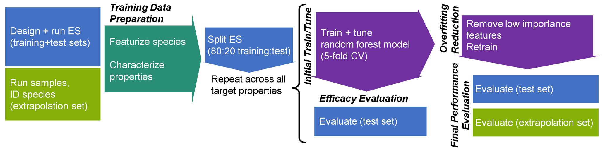
Figure 1 Analytical pipeline for chemical properties modeling using a random forest model. ES indicates the external standard; CV indicates the cross-validation.

3.1 Featurization, feature selection, and target selection

As the aim of this work is to develop methods that can be applied to novel species not included in mass spectral databases, features utilized in this analysis rely solely upon the information readily available for unidentifiable species. Given the size and complexity of the intended use data suites, features must also be automatically generatable from the instrument data output and not rely upon any visual or manual categorization by researchers. In order to make these models more broadly useful to the atmospheric community, less common features produced by the GCxGC-MS instrumental setup (e.g., second-dimension retention time and high-resolution spectra) are not utilized for chemical properties modeling in order to increase the method's applicability to single dimension GC-MS systems and instruments with lower-resolution mass spectra.

3.1.1 Mass spectral featurization

The only chemical information directly produced by GCxGC-MS for unidentified organic species are their locations in GCxGC volatility–polarity space and mass spectra. These sources of information are therefore exclusively utilized in creating and selecting the features for chemical properties modeling. The retention index of each compound was directly utilized as a feature, but the mass spectra require interpretation in order to be used.

The unit mass resolution spectra utilized in this analysis include each charged fragment represented by its measured mass to charge ratio ($m/z$) and a relative signal score out of 1000 (normalized by the most abundant fragment's peak signal). EI is a high-energy or hard ionization technique which typically leaves only a small fraction of molecular ions intact and creates positively charged ion fragments that are almost all singly charged, with any multiply charged ions at extremely low abundance. This means that the molecular formulae cannot generally be directly determined from the mass spectrum, even when the spectra are high resolution, and measured ions can be assumed to have a single charge. That said, the $m/z$ of charged fragment ions yield useful information into chemical characteristics and functional groupings that can provide critical chemical information; for example, a peak at $m/z=\mathrm{73}$ corresponds to a fragment of Si(CH₃)${}_{\mathrm{3}}^{+}$, a derivatization fragment which indicates that the ionized compound contained an OH group which was derivatized (see Sect. 2.3). The mass differences between charged peaks also represent important pieces of information, as they can indicate losses of uncharged molecular fragments that similarly point to the structure and characteristics of the original compound. It is important to note that not all neutral mass differences between charged peaks can be interpreted as direct neutral losses, as not all high $m/z$ charged fragments directly fragment onto lower $m/z$ charged fragments in a manner that can be directly interpreted from neutrally charged fragment losses. However, frequently occurring neutral differences may still hold value in reflecting a common coordination of neutral loss processes.

The greatest chemical information lies in features that exist in an intermediate range of occurrence frequency in the data set. A feature which appears in all the training species does not provide any useful information in predicting properties of the test species. Neither does a feature which is totally unique to a single species, as it does not provide any information on patterns which can be used to adjust prediction of properties for other species. This logic can be applied to mass spectral featurization; while it would be possible to convert every $m/z$ to a feature and so input the entire raw mass spectrum of each compound as a series of features for the random forest model, this approach would be inefficient, open to error introduced by noise, and miss the important information provided by neutral mass differences between charged fragments.

Multiple approaches for mass spectral featurization were tested to optimize the number of features and representation of features. Given the final choice in model structure (random forest; as described in Sect. 4), the inclusion of co-varying features or more features than necessary did not introduce significant sources of error. Target-specific feature restriction based on importance is discussed in Sect. 4. The final mass spectral featurization method selected for this analysis, a simplified adaptation of methodology described in Eghbaldar et al. (1998), was as follows: the top five charged fragments (mass spectral peaks) from each training set mass spectrum are selected. The mass differences between these five peaks (a maximum of 10 numbers, if all fragments occur at differently spaced $m/z$) were then compiled into a list of neutral losses. The charged fragment lists and the neutral loss lists of all training set external standard compounds were next combined in a frequency list, with each charged fragment or neutral loss quantified by frequency (how many compounds in the external standard test set exhibited that charged fragment or neutral loss among their top five peaks). The top 40 most common charged fragments and top 20 most common neutral losses were converted into features. The identities of these 40 most common fragments and 20 most common neutral mass differences (along with possible identities and notes) can be found in Tables A2 and A3, respectively. The mass spectra of all training, test, and extrapolation set compounds were then simplified using the previously described method (top five peaks extracted and mass differences between those peaks calculated). Each $m/z$ feature was assigned the normalized signal of that peak in the mass spectrum if the feature $m/z$ was one of the top five peaks; otherwise, it was set to zero. Each neutral loss feature was assigned true or false for each compound, depending on whether the neutral loss appeared in the mass differences between the five most significant peaks. An example mass spectral featurization for the example compound hexadecane can be found in Table A4, and the mass spectral featurization process is included in the open-source R script accompanying this publication.

3.1.2 Target selection for chemical properties modeling

The goal of chemical properties modeling is to enable the inclusion of unidentified species in aerosol organic analysis that has previously been restricted to species for which the identity or at least chemical formula is known. One way in which complex organic mixtures are visualized and analyzed is through orientation of observed species in chemical properties spaces that have been developed and broadly utilized in the field of aerosol science. Of these space, two include the volatility basis set (VBS; Donahue et al., 2006) and the visualization by average carbon oxidation state and carbon number developed in Kroll et al. (2011), hereafter referred to as $\stackrel{\mathrm{‾}}{{\mathrm{OS}}_{\mathrm{c}}}$-n_c space. Compounds can be plotted in VBS space by their O : C or $\stackrel{\mathrm{‾}}{{\mathrm{OS}}_{\mathrm{c}}}$ (average carbon oxidation state; Kroll et al., 2011) against some measure of volatility, either log(vapor pressure) or log(C₀), where C₀ is the pure component sub-cooled liquid vapor pressure in the atmosphere. In $\stackrel{\mathrm{‾}}{{\mathrm{OS}}_{\mathrm{c}}}$-n_c space, compounds are plotted by their average carbon oxidation state ($\stackrel{\mathrm{‾}}{{\mathrm{OS}}_{\mathrm{c}}}$) against carbon number. The ability to map novel or unidentifiable compounds in these spaces would provide critical information about the properties of the individual species, enable identification of groups of chemically distinct novel compounds deserving particular consideration, and more completely visualize the distribution of chemical characteristics for complex mixtures and potential routes of chemical transformation (e.g., oligomerization, functionalization, and fragmentation) beyond the identifiable components. With these goals in mind, the properties selected to be the targets of these modeling efforts were number of carbons (n_c), O : C, $\stackrel{\mathrm{‾}}{{\mathrm{OS}}_{\mathrm{c}}}$, and vapor pressure.

Carbon number, O : C, and $\stackrel{\mathrm{‾}}{{\mathrm{OS}}_{\mathrm{c}}}$ (based on the equation in Kroll et al., 2011) can all be directly calculated from a chemical formula, which was known for each standard and ambient extrapolation compound (see Sect. 3.2). Vapor pressure is not directly calculable from a chemical formula, and not all identified compounds in the external standard and extrapolation data sets have reliable experimental vapor pressure measurements available, so structurally based vapor pressure predictions are utilized instead. Isaacman-Vanwertz and Aumont (2021) find that, of all the structure-based vapor pressure prediction methods available, the average of predictions generated by the EVAPORATION (Compernolle et al., 2011), Nannoolal (Nannoolal et al., 2008), and Simpol (Pankow and Asher, 2008) models yields the most accurate vapor pressure prediction. These methods were therefore utilized to predict the vapor pressures of all standard and extrapolation set compounds, and the average structurally predicted vapor pressures were utilized as the true vapor pressures for model training and evaluation. In total, 7 of the external standard test set species and 15 of the extrapolation set species were incompatible with the prediction capabilities of one or more of the three structural vapor pressure prediction methods (most frequently due to functional group types for which the models are not parameterized) and were therefore not utilized in the performance analysis. There were two additional potential targets, namely double bond equivalent and H : C ratio, that were tested but failed to produce sufficiently robust property predictions.

The final components of the chemical properties random forest models are as follows:

• Targets – carbon number, $\stackrel{\mathrm{‾}}{{\mathrm{OS}}_{\mathrm{c}}}$, O : C, and vapor pressure (structurally modeled).

• Features – retention index, 40 feature representation of mass spectral charged fragments, and 20 feature representation of neutral mass differences between charged fragments.

A table listing the entire set of input features for chemical properties modeling of the example compound hexadecane can be found in Table A4, and the instrument-produced mass spectrum for this species can be found in Fig. A1.

3.1.3 Featurization and target selection for quantification modeling

The compound quantification factor is significantly and reliably related to retention index across all compound classes tracked, but this relationship is not linear and changes much more rapidly in some retention index windows than others. This phenomenon, caused by incomplete cold inlet trapping of species in the most volatile sensitivity region and incomplete thermal desorption of species in the least volatile sensitivity region, is illustrated in Fig. A2 and is consistent with findings presented in Zhang et al. (2018). A variety of retention index corrections were tested, including the following: (a) factorizing the retention indices of each compound (rounded to the nearest 100) and including the results as a feature in model training and testing and (b) normalizing (dividing) each compound by the raw signal of its nearest deuterated alkane internal standard, with the method utilized in Zhang et al. (2018). Both methods, however, performed poorly in the 1600–1900 RI range, where response increases extremely rapidly with RI (Fig. A2). The most reliable normalization method, and the method selected for this analysis, was normalizing (dividing) all compound quantification factors by the average response curve for alkanes, defined by the combination of two best-fit exponential curves, which intersect at RI ≈ 1950, as illustrated in Fig. A2, and training on/predicting this normalized response factor rather than the raw quantification factor. The r² of the exponential fit of individual calibration period quantification factors around the response curve in the volatile region is 0.77, while the r² of the curve describing the less volatile region is 0.65. Note that these fits take into account each quantification factor of each calibration window and are therefore influenced by the variations in the measured quantification factors of the same compounds measured at different points throughout analysis. RI-normalized response factors were translated back to predicted quantification factors for performance evaluation, as other methods of quantification do not utilize this normalization method.

Unlike the case of chemical properties modeling, quantification modeling performance was significantly improved by inclusion of second-dimension retention time information, and it was therefore included as a feature in the response factor prediction. As a result, this approach in its current form is only usable by GCxGC-MS applications but could be adapted to single-dimension chromatography–mass spectrometry.

In this analysis, continuous measurement periods (consecutively collected samples) were analyzed in sequences bounded by calibration curve runs. To preserve the quantification continuity in these consecutive measurements and to avoid step changes in calculated concentration that might occur due to switching between quantification factors, the two quantification factors bookending an analysis period are averaged to assign the quantification factors for samples run in that interval. To replicate this approach, the compound quantification factors were sequentially averaged to yield five quantification periods (the final calibration curve experienced an instrument failure, and the last calibration period is therefore based solely on the final curve).

The mass spectral featurization is described in mass spectral featurization above.

The final components of the quantification model are as follows:

• Target – normalized response factor (RI curve normalized and calibration period averaged).

• Features – retention index, second-dimension retention time, calibration period, 40 feature representation of mass spectral charged fragments, and 20 feature representation of neutral mass differences between charged fragments.

3.2 Training, test, and extrapolation set curation

To generate a training and test set from the external standard data, each external standard was assigned to a chemical group (alkane, sugar, PAH, etc.), and the list of external standard compounds was randomly split 80 : 20 (80 % of compounds in the training set and 20 % in the test set) maintaining the ratios of different chemical groups. In total, 200 possible splits were generated, and the split which demonstrated the greatest similarity in median retention index and median second-dimension retention time between the test and training sets was selected to avoid potential extrapolation problems that might occur with a highly skewed distribution of test and training compounds across the GCxGC space. This process is documented in the Supplement.

Figure 2 Distribution of training, test, extrapolation, and unidentified sample compounds in two-dimensional chromatographic chemical properties space.

The extrapolation set was curated from the compounds isolated from the GoAmazon samples by comparing the spectra and retention indices of compounds to the external standard and matches in the NIST14 mass spectral database. Of the ∼ 1500 unique compounds identified across 11 template samples, 63 were determined to match external standard compounds, and an additional 71 compounds were identifiable from the NIST library due to a high (> 800, Worton et al., 2017) mass spectral match factor and retention index agreement with database entries. Based on number of silicon atoms in the assigned formulae from the NIST identification, each chemical formula was converted to its underivatized form. Only the 71 compounds that were identifiable from the NIST library but not from external standards were included in the extrapolation set to ensure that performance metrics for the extrapolation set would not be skewed by the inclusion of species that may have been in the training data and to ensure that the test set and extrapolation set performance evaluations would be entirely independent. The methodology described in this work cannot effectively extrapolate beyond the feature space of the training data set, and the identifiable organic compounds in the Amazonian aerosol samples are defined as an extrapolation set, not because they test the abilities of the model to extrapolate beyond the feature space boundaries of the external standard training data but because they represent the true range of individual isomer-specific identities observed in ambient samples. These compounds test the model's ability to extrapolate property prediction beyond the compound groups included in the external standard and indicate whether the sample is sufficiently similar to the training data to make this approach appropriate for the target sample medium, as extremely high prediction inaccuracies indicate compound classes too dissimilar from the training data to be appropriately modeled using Ch3MS-RF (Chemical Characterization by Chromatography–Mass Spectrometry Random Forest Modeling). As illustrated in Fig. 2, the distribution of training, test, and extrapolation set species utilized in this work effectively span the distribution of unknown compounds in GCxGC volatility–polarity space.

4 Model selection, training, and tuning

The number and complexity of input features and lack of clear linear relationships between target properties and input features in this analysis is well suited to a decision-tree-based analytical approach (Bentéjac et al., 2021; Rokach, 2016). Random forest and gradient boosting methods were both preliminarily tested for response factor prediction. Random forests demonstrated slightly better performance and were selected for this and additional methodological reasons, as follows. Random forests are more robust to overfitting than gradient boosting, which is a particular concern in this case, given the small number of training compounds (∼ 100) compared to the large numbers of novel environmental organics that are the intended subjects of unverifiable modeling. Additionally, random forests perform well when using the default settings and do not require extensive tuning to achieve optimal performance (Bentéjac et al., 2021). As the aim of this work is to produce models that the atmospheric science community, including non-experts in machine learning, can easily implement for novel compound analysis, this robustness and simplicity is a significant advantage.

Table 1 Tuning parameters and important features for chemical properties prediction models. $m/z$ indicates charged fragment features, and n indicates neutral mass difference features. Note: tree diversity feature restriction parameter is mtry.

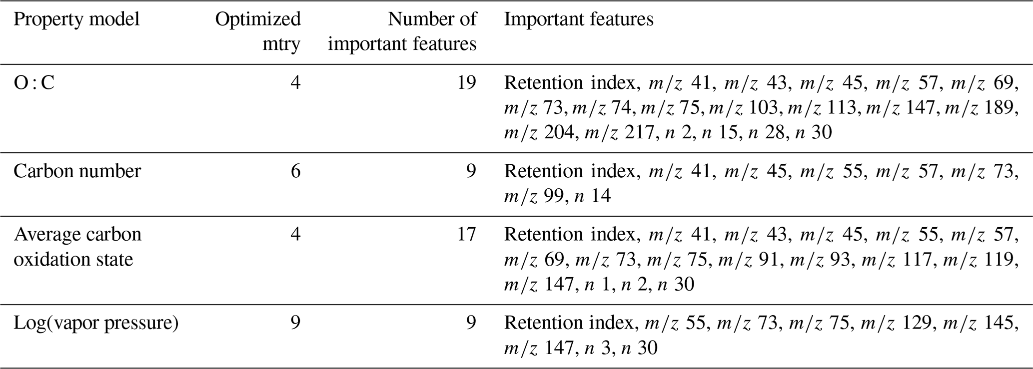
The training and tuning processes for chemical properties prediction are visualized in Fig. 1. For each target property, the model was trained on the external standard training set data, the curation of which is described above. As previously referenced, random forests do not require extensive tuning, and for ease of use reasons, most parameters were maintained at their default values. Tuning primarily focused on feature restriction. Feature restriction to enforce tree diversity (mtry) was optimized by five-fold cross-validation, with the mtry value that minimized mean absolute error (MAE) selected. Although random forest modeling is comparatively not influenced by the inclusion of features that do not contribute significant predictive capabilities, the inclusion of unnecessary features can contribute to overfitting of the training data, which decreases the prediction performance for the test and extrapolation data sets. To address this problem, the feature importance (a measure of increase in node purity when this feature is used in a split) of each input feature was extracted from the original predictive model. The importance metrics were normalized by the total importance of all features to generate a percent importance score for each feature. Importance distributions were highly skewed, with a relatively low number of features contributing the majority of decrease in node purity. Features that contributed less than 1 % to the total importance score were removed, and the model was retrained on only the important features. Extrapolation set performance improvements from removal of low importance features was low, with an improvement in OSR² (out-of-sample R², defined in detail in Sect. 5.1) of the order of 0–0.03. This indicates that this step is not crucial for chemical properties or quantification factor prediction. The cross-validation-optimized mtry number, number of important features, and identity of important features for the chemical properties models (one optimized model per property predicted) are summarized in Table 1. For quantification modeling, mtry is optimized at 44 features, and 46 features meet an importance criterion of > 1 %.

5 Model performance evaluation

5.1 Chemical properties modeling performance

There are three performance metrics utilized to evaluate target predictions for the four chemical properties models. The first, out-of-sample r² (OSR²), provides a measure of how significantly a model improves upon a baseline assumption that all target property values are equal to the mean of those values in the training data. It approaches a maximum of one for perfect predictions. The second metric, mean absolute error (MAE), provides the mean absolute prediction residual in the units of the target property. This metric is particularly important, as it provides a benchmark for prediction accuracy which can be translated into visualization and utilized to determine which applications are appropriate given prediction errors. The final performance metric, root mean square error (RMSE), is also a scale-dependent error metric and provides the quadratic mean of prediction residuals. The equations for these metrics are provided below:

$$\begin{array}{}\text{(1)}& {\displaystyle }{\mathrm{OSR}}^{\mathrm{2}}=\mathrm{1}-{\displaystyle \frac{\sum _{i=\mathrm{1}}^n{\left(T_i-P_i\right)}^{\mathrm{2}}}{\sum _{i=\mathrm{1}}^n{\left(T_i-{\stackrel{\mathrm{‾}}{R}}_T\right)}^{\mathrm{2}}}}\text{(2)}& {\displaystyle }\mathrm{MAE}={\displaystyle \frac{{\sum }_{i=\mathrm{1}}^n\left|P_i-T_i\right|}{n}}\text{(3)}& {\displaystyle }\mathrm{RMSE}=\sqrt{{\displaystyle \frac{{\sum }_{i=\mathrm{1}}^n{\left(P_i-T_i\right)}^{\mathrm{2}}}{n}}}.\end{array}$$

In this notation, for each test or extrapolation set compound i summed across a population of n compounds, T_i indicates the true value of the property being tested, P_i indicates the predicted value of that property, and ${\stackrel{\mathrm{‾}}{R}}_T$ indicates the mean of the selected property in the training data set.

Table 2 Performance metrics for random-forest-based modeling of chemical properties of the external standard test set. Range of true properties units in units of the property O : C, in unitless atom number : atom number, carbon number in atom number, average carbon oxidation state in mean charge, and log(vapor pressure) in log(atm).

Table 3 Performance metrics for random-forest-based modeling of chemical properties of the ambient aerosol sample extrapolation set. Range of true properties units in units of the property O : C, in unitless atom number : atom number, carbon number in atom number, average carbon oxidation state in mean charge, and log(vapor pressure) in log(atm).

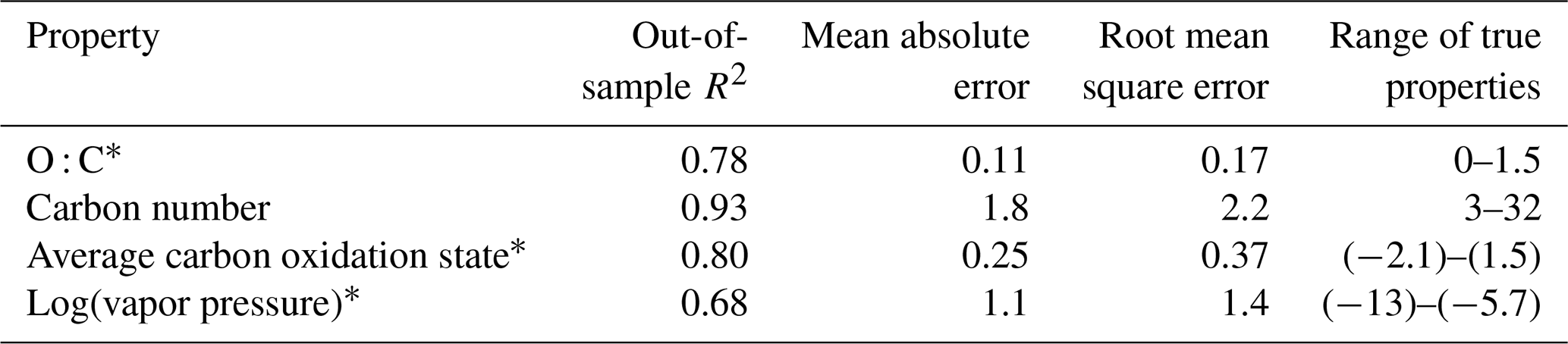
^∗ Restricted to the retention index > 1500.

The prediction performance for the tuned and trained chemical properties model are evaluated independently on both the external standard test set (Fig. 3; Table 2) and the ambient sample extrapolation set (Fig. 4; Table 3). Both of these performance evaluations are important for different reasons. The external standard contains many series of highly chemically similar species (for example, alkane and carboxylic acid series), meaning that the test set is likely to be more chemically similar to the training set than a real distribution of ambient organic species would be. Performance evaluation on the extrapolation set therefore provides a more realistic assessment of likely prediction accuracies on the large number of novel ambient organic compounds that are the intended focus of this modeling effort. That said, prediction performance on the external standard test set also yields important information. The external standard is designed to cover the entire space of anticipated chemical features for the environmental samples and is therefore more diverse relative to the number of compounds included compared to the extrapolation set (which is primarily CHO-type compounds). Performance evaluation on the external standard test set therefore yields more information about model performance across a broad suite of compound classes.

Figure 3 External standard test set of true and predicted chemical properties from random forest modeling.​​​​​​​

Figure 4 Ambient extrapolation set of true and predicted chemical properties from random forest modeling.

5.1.1 Test set performance evaluation

By all evaluation metrics applied (summarized in Table 2), performance for carbon number, O : C, carbon oxidation state, and log(vapor pressure) predictions on the external standard test set are robust. The O : C and carbon number predictions are particularly strong, with OSR² of 0.89 and 0.88, respectively, and mean absolute errors of 0.072 element ratio units and 1.8 carbon number units. For context, given the range in true values from O : C = 0–1 and carbon number = 4–31, both mean absolute errors are approximately 7 % of the range of measured values. For $\stackrel{\mathrm{‾}}{{\mathrm{OS}}_{\mathrm{c}}}$ and vapor pressure, the mean absolute errors normalized by the measurement range are both approximately 12 %. As illustrated Fig. 3, this means that the distribution of predicted properties usefully and reliably reflects the distribution of true properties and indicates that the random-forest-based model provides useful information that allows a wide range of compound classes to be reliably characterized based on the mass spectrum and retention index.

5.1.2 Extrapolation set performance evaluation

As discussed above, while the external standard test set provides useful information on model performance across a wide range of compound types, its performance is potentially inflated by a high degree of chemical similarity between the training and test set compounds. Performance evaluation on the ambient sample extrapolation set is therefore likely a more accurate indicator of prediction performance on novel or uncataloged species. Of the four properties modeled, the performances for carbon number prediction and carbon oxidation state remain consistent or improve slightly (carbon number OSR² increases to 0.93), while O : C and log(vapor pressure) prediction performances decrease, both in terms of OSR² and MAE (Table 3).

The weakest extrapolation set performance by far is vapor pressure prediction, which drops to OSR² of 0.68. The correlation between predicted and true properties is also the weakest (as illustrated in Fig. 4), with particularly large prediction residuals for the highest volatility species. For example, the extrapolation set compound with the highest vapor pressure prediction error is 1,2-Benzenedicarboxylic acid, which has a retention index of < 1400, making it more volatile than the most volatile internal standard compound. While this compound does not lie outside of the volatility and polarity boundaries of the external standards in GCxGC space, is significantly more volatile than any diacid compound in the standard mixture, and the influence of double derivatization on its true ambient volatility relative to the chromatographic elution time of its derivatized form may not have been appropriately captured. Unlike the other properties targeted in this analysis, vapor pressure is not directly calculable based on chemical formula and poses challenges for many techniques; as discussed in Isaacman-Vanwertz and Aumont (2021), molecular structure plays an important role in volatility, which significantly limits the accuracy with which techniques that identify formula but not structure (typically chemical ionization techniques) can predict the true volatility of their measured components. A more complete comparison between the random forest model's performance in vapor pressure prediction compared to other techniques used throughout the field is therefore required to provide context for vapor pressure prediction errors in the ambient sample extrapolation set (further discussed below in Sect. 5.1.3).

For both O : C and $\stackrel{\mathrm{‾}}{{\mathrm{OS}}_{\mathrm{c}}}$ (which are highly related properties), extrapolation set prediction performance suffers at the high end of the oxygenation scale, although the performance reduction is far more pronounced for O : C prediction. This is due to the lack of highly oxygenated species in the external standard; random forest models do not extrapolate beyond the range of properties in the training data and therefore cannot predict O : C ratios of higher than 1.5 when that is above the maximum in the training data. The extraneously highly oxidized species for which O : C and $\stackrel{\mathrm{‾}}{{\mathrm{OS}}_{\mathrm{c}}}$ prediction accuracy suffers lie almost exclusively in the most volatile region instrument sensitivity, where vapor pressure prediction inaccuracies have been previously described. As a result, extrapolation set property prediction for O : C, $\stackrel{\mathrm{‾}}{{\mathrm{OS}}_{\mathrm{c}}}$, and log(vapor pressure) were restricted to compounds above a retention index of 1500. As illustrated in Figs. A3 and 2, the significant majority of ambient analytes were above the 1500 retention index threshold, justifying the decision to restrict the prediction of these properties to the retention index window in which their performance is better optimized. In applying these techniques to the larger suite of novel species, maintaining these retention window restrictions is critical to avoid the introduction of significant sources of error.

Given the strong and consistent performance of carbon number and $\stackrel{\mathrm{‾}}{{\mathrm{OS}}_{\mathrm{c}}}$ predictions across the majority of the retention index space and between both test and extrapolation sets, the most robust visualization of chemical properties based on random forest predictions is likely to be in $\stackrel{\mathrm{‾}}{{\mathrm{OS}}_{\mathrm{c}}}$-n_c space (Kroll et al., 2011). Predicting the carbon numbers and $\stackrel{\mathrm{‾}}{{\mathrm{OS}}_{\mathrm{c}}}$ of the known ambient compounds and superimposing the true and predicted property distributions in the $\stackrel{\mathrm{‾}}{{\mathrm{OS}}_{\mathrm{c}}}$-n_c space highlights the strengths and weaknesses of chemical properties modeling. To better represent the prediction capabilities of the full chemical space and the scope of information that would be provided for properties prediction on a complex sample including hundreds of individual species, all identifiable ambient compounds (including those that overlap with the external standard) were included in property prediction and visualization. As illustrated in Fig. 5, the real and predicted chemical properties spaces for the ambient data set indicate both strengths and weaknesses for this application of chemical properties modeling. As noted earlier, random forest modeling does not extrapolate and has a tendency to underpredict property extremes. This is apparent in both the high $\stackrel{\mathrm{‾}}{{\mathrm{OS}}_{\mathrm{c}}}$ region and the high carbon number regions of the $\stackrel{\mathrm{‾}}{{\mathrm{OS}}_{\mathrm{c}}}$-n_c space, where high carbon oxidation states and high carbon numbers were each independently underpredicted. These errors could be moderated by adding more oxygenated species and higher carbon number species to the external standard, which would provide the model with more information to predict properties in these regions. In a context of an extended continuity of analysis of similar sample media, this suggests an iterative approach in which the addition of new standards to a calibration mixture can be prioritized through analyzing the chemical features of poorly predicted compounds in the sample media and adding new standards that replicate those features. Despite the prediction errors visualized in Fig. 5, the overall shape of the true chemical properties space was extremely well represented by the predictions. While conclusions based on the presence or absence of extremes in predicted properties would not be appropriate, analyses based on the relative distributions of populations of interest provide valuable insight comparable to other parameterizations of compound properties from incomplete knowledge.

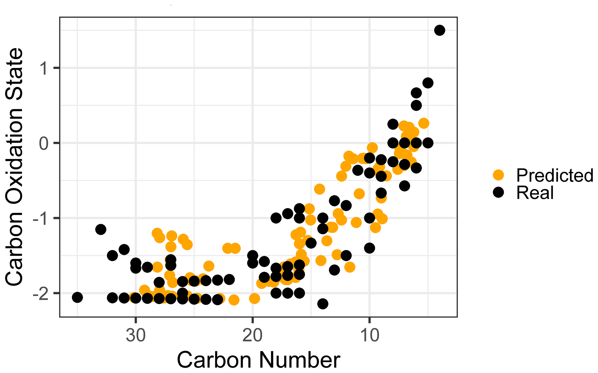
Figure 5 True versus predicted chemical properties distribution of ambient sample organic species within a carbon number vs. carbon oxidation state space.

5.1.3 Vapor pressure modeling: comparison to prior methods

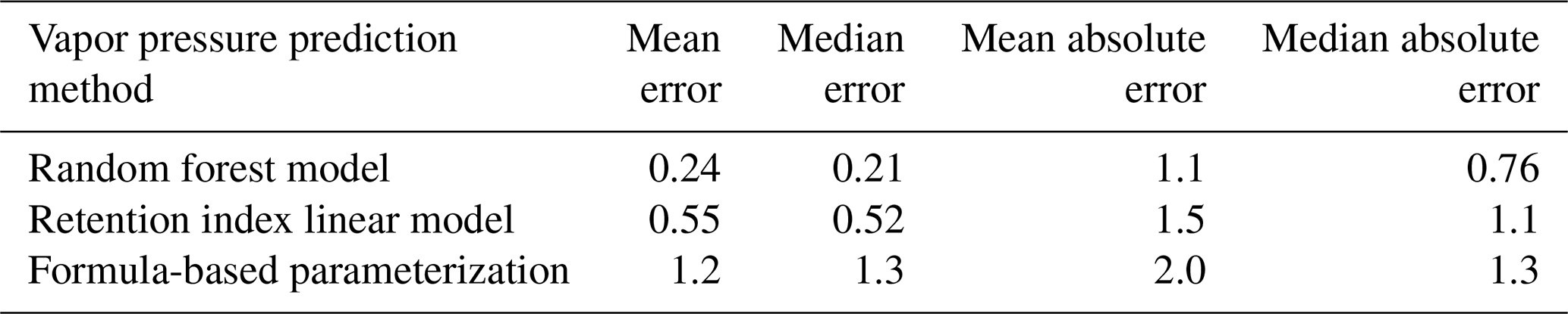
Chromatography using a non-polar column is intended to separate compounds by volatility and has been used to directly predict novel compound vapor pressures in previous studies (Isaacman-VanWertz et al., 2016). It is therefore important in this context to evaluate both how significantly random forest modeling improves upon the simple linear modeling of volatility based on retention index and how this method compares to other parameterizations of vapor pressure. As illustrated in Fig. 6 and Table 4, the log(vapor pressure) prediction residuals for random forest model predictions indicate that random-forest-generated predictions are both more accurate and more precise than predictions by the linearized retention index method or from the Li et al. (2016) chemical-formula-based parameterization, as they demonstrate a tighter distribution that is more centered around zero. The mean absolute error for random forest vapor pressure prediction is significantly lower than errors from both predictions based on retention index (t test p value = 0.01) and predictions based on chemical formula (t test p value = 3.1 × 10⁻⁵).

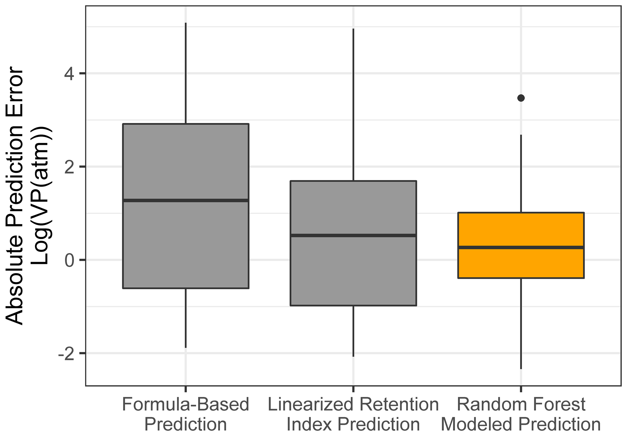
Figure 6 Vapor pressure prediction residuals (log(vapor pressure); vapor pressure in the atmosphere) for vapor pressure predictions of the ambient extrapolation set based on formula-based parameterization (Li et al., 2016), linearized retention index-based modeling, and random forest modeling.

Table 4 Error distribution metrics random forest model, retention index linear model, and formula-based predictions of vapor pressure. All reported errors in units of log(vapor pressure(atm)).

5.2 Quantification modeling performance

The approach for evaluating the performance for quantification modeling requires slight alterations compared to property prediction. Although the random forest model predicts the residuals of quantification factors around the retention index response normalization curve (Fig. A2) rather than doing so directly, these residuals are converted back to quantification factors for both the true and predicted properties for performance evaluation. This serves two purposes; first, other quantification methods do not use this retention-index-based normalization, so conversion to absolute prediction errors is necessary to compare methods, and second, a direct quantification error assessment provides more useful and applicable information about how significantly quantification errors could influence conclusions based on model-quantified data.

The test set compounds were quantified using two alternative quantification methods, i.e., manual or closest proxy quantification (described in Liang et al., 2021, which utilizes a combination of both), to benchmark random forest model performance. Manual proxy quantification entails manually assigning a compound to a chemically similar external standard based on researcher judgment on what chemical class the unidentified compound would likely belong to, based on some combination of location in GCxGC space and mass spectrum. This is the current preferred method for the quantification of compounds that are not in the external standard and, in theory, should provide the most reliable results in cases where an extremely chemically similar standard is available, but it is highly inefficient and relies upon researcher judgment calls, which are difficult to standardize. Closest proxy quantification assigns each compound to its nearest external standard in GCxGC space or to an average of the nearest standards within a set radius limitation. In this work, the average of the quantification factors of the three nearest standard species was used, as this demonstrated improved performance compared to single closest proxy quantification. This method is efficient, but it introduces potentially significant error by assigning species with different chemical characteristics (and therefore different quantification factors) to the same response factor if they are sufficiently close in GCxGC space. Each test set compound was assigned to a proxy quantification factor from the training set based on each of these two methods, and each proxy compound's quantification factor at each time point was substituted as a prediction of the test set compound's quantification factor at that calibration window.

Table 5 Performance metrics for quantification factor prediction for three methods of unidentified compound quantification, i.e., random forest modeling, manually assigned proxy quantified, and closest proxy quantified.

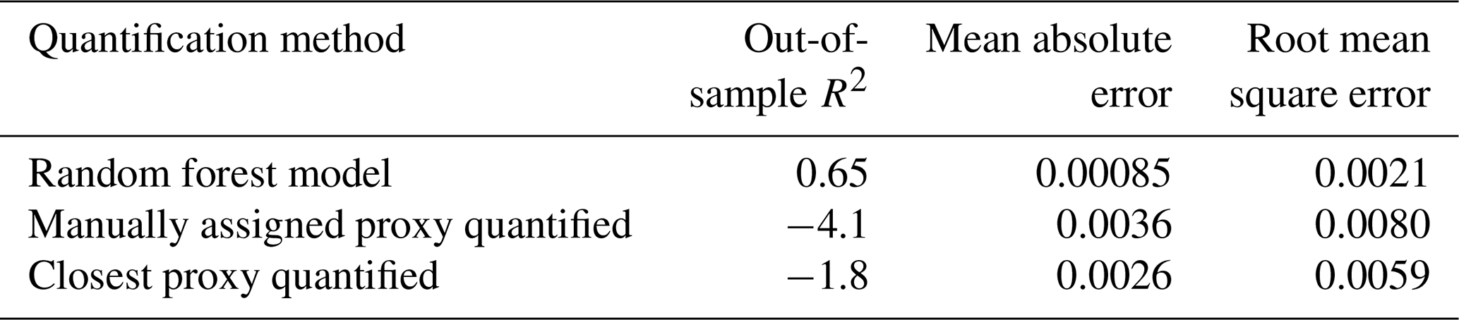
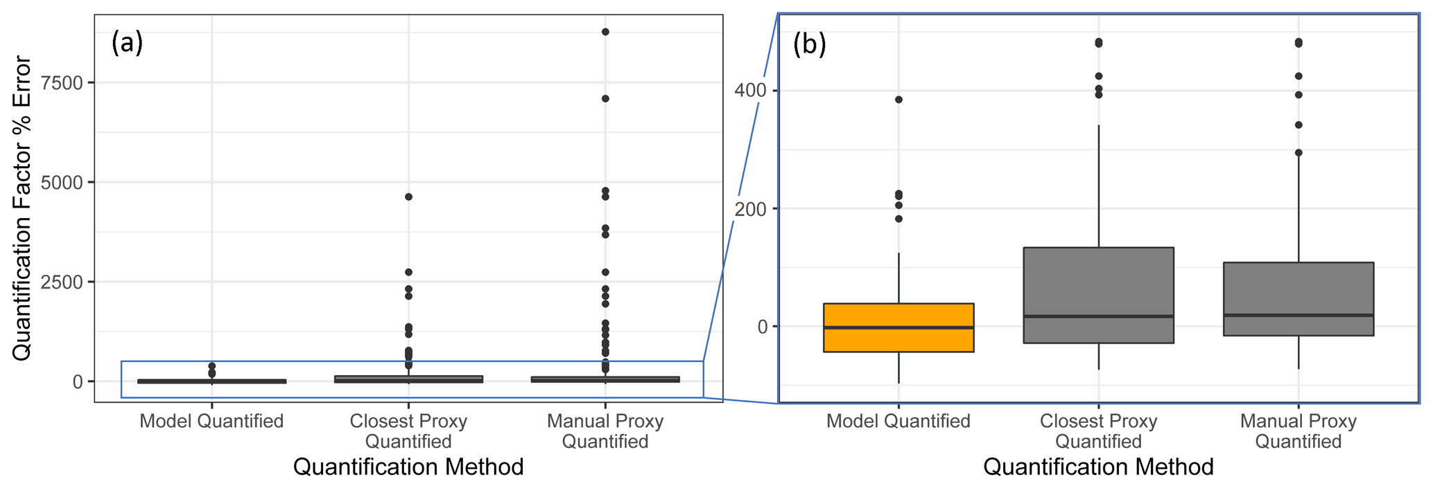
Figure 7 Quantification performance comparison between the random forest model (orange) and two previously utilized quantification methods, specifically the closest proxy quantification and manually assigned proxy quantification. The midline of the boxes indicates the sample median, while the top and bottom indicate the 25th and 75th percentiles. Linear whiskers extend to the least extreme values within 1.5 × of the inner quartile range of the sample. Disconnected dots indicate the sample outliers that fall beyond the whisker parameters.

The standard performance metrics for quantification factor prediction using the random forest model, manual proxy quantification, and closest proxy quantification are compared in Table 5. The random forest model significantly outperforms both other methods; it has a relatively high OSR² of 0.65 compared to negative OSR² values for the two proxy methods (indicating that at least on average, assuming all test compounds have the same quantification factor, the average of all training set compounds would have performed better than proxy quantification). MAE and RMSE also indicate improved performance when using the random forest model over other methods. While these metrics provide useful information on model performance, they do not reveal why the performance (particularly of the proxy methods) is so poor and do not provide useful information to evaluate likely propagation of quantification errors. Unlike for the chemical properties modeling, for quantification modeling the percent error is a much more important metric than absolute error because it translates directly to how significant total the quantification error across a large suite of compounds is likely to be and provides insights into underlying biases in different methods. Figure 7 illustrates the quantification factor percent error distributions of the three methods and demonstrates the improved performance of random-forest-modeled quantification predictions on three criteria. First, as illustrated by Fig. 7a, random forest modeling produces far fewer and less extreme outlier prediction errors that are orders of magnitude different from the true values. These result when a compound that the instrument is extremely insensitive to (which would have a true extremely low quantification factor) is assigned a moderate or high quantification factor. In practice, the influence of these types of quantification inaccuracies is very limited, as the few ambient species that the instrument is this significantly insensitive to would occur above detection limits, but they could introduce errors nonetheless. Here it is important to keep in mind that each point represents a single quantification from a single calibration period; some outliers therefore indicate compounds that exhibited extremes in quantification factors during a single calibration period. This was most common among standard compounds at the edges of the instrument's sensitivity window, as these species are more significantly impacted by alterations in instrument performance. Second, as illustrated by Fig. 7b, the error distribution for the random forest model is significantly more centered around zero compared to either proxy model. The median random forest model quantification error is −2 %, compared to 17 % for closest proxy quantification and 19 % for manual proxy quantification. In practice, this indicates that over a large number of quantified species, random forest modeling is unlikely to introduce biased quantifications that might skew results, while the two proxy methods would likely inflate the apparent mass of novel compounds. Third, also illustrated by Fig. 7b (though less directly), random forest modeling produces prediction errors more tightly distributed around the median, meaning that the absolute percent error distribution for random forest modeling also outperforms the two proxy methods. Median absolute percent error for random forest model predictions is 37 %, compared to 57 % for the closest proxy method and 41 % for the manually assigned proxy method. The average percent error improvements from random forest modeling compared to both proxy methods are statistically significant (t test p values both < 0.0004), but the median absolute percent error distributions of the random forest and manually assigned proxy quantifications are not significantly different based on a Mood's median test. The random forest and closest proxy method absolute percent error distribution differences are statistically significant, with a Mood's test p value of 0.001. While critical for contextualizing the potential impact of quantification errors on mass attribution of complex mixtures, a percent-error-based analysis of prediction accuracy is necessarily asymmetrical, as a predicted quantification factor can produce a minimum of −100 % error (the case if the predicted value were to be zero) but far more than +100 % error if the quantification factor is significantly overpredicted. A symmetrical error analysis of log(predicted quantification factor/true quantification factor), illustrated in Fig. A4, is required to probe the frequency and dynamics of underprediction in greater depth. Figure A4 demonstrates that the random forest model is more prone to underprediction outliers but continues to outperform the other methods in achieving a narrow error distribution centered at zero.

A final benefit of a random-forest-modeling-based quantification not captured in the performance metrics is the ability to utilize incomplete data. With proxy quantification, any standard compound that cannot be calibrated for at any point over the course of an analysis cannot be used, as the species that are calibrated by that compound would not be quantifiable during the window with missing calibration data. The random-forest-based quantification method relies upon the entire external standard suite to inform corrections for instrument performance over time and can therefore produce robust quantification factor predictions, even when individual standard calibration curves are missing for a particular calibration window. This allows for significantly greater flexibility in analysis, as compounds can be added to the external standard if they are observed in initial samples and still be usable to inform quantifications for periods before they were present.

In summary, random forest quantification factor modeling significantly outperforms both closest proxy and manual proxy quantification methods. It is significantly more efficient than manual proxy modeling, exhibits fewer outliers of multi-orders of magnitude overestimations, produces an error distribution that is more centered around zero (preventing significant biases in total mass over large numbers of quantified and summed species), and exhibits improvements in absolute percent error of predictions.

5.3 Considerations for adaptation across instruments and methods

The approach presented in this work prioritizes continuity between training, test, and sample data by exclusively training the model on data produced by a single instrument using a standardized methodology. This approach was selected to ensure that the patterns identified by Ch3MS-RF in the training data were as directly relevant as possible to the unidentifiable sample compounds of interest. However, in some cases, accumulation of a representative external standard spanning the entire feature domain of the unidentifiable compounds of interest may not be practical or possible. Electron ionization (70 eV) mass spectrometry is an extremely well characterized and consistent technique, but chromatographic retention times and indices can vary. In order for data produced by multiple instruments and techniques to be integrated within Ch3MS-RF, it is therefore important to establish the tolerance of prediction performance to drifts in the retention index.

To test sensitivity to the retention index or retention time shifts across instruments and methods, the vapor pressure, carbon number, $\stackrel{\mathrm{‾}}{{\mathrm{OS}}_{\mathrm{c}}}$, and O : C of the external standard test set compounds were predicted using retention index inputs that were shifted from their observed retention indices. A broad range of shifts from −200 (indicating the equivalent of a two-carbon number shift; for example, if in the test sample heptadecane were to elute at the time that pentadecane eluted in the training standard run) to +200 were tested (including −200, −150, −100, −50, −25, +25, +50, +100, +150, and +200). A new mean absolute error was calculated for each set of predictions based on the shifted retention indices and compared to the unshifted mean absolute error to calculate the percent increase in mean absolute error as a function of test set retention index shift. These results are visualized in Fig. 8. The two measures of oxidation, $\stackrel{\mathrm{‾}}{{\mathrm{OS}}_{\mathrm{c}}}$, and O : C were relatively insensitive to retention index shifts, as their mean absolute errors increased by less than 10 % at a retention index shift of ±200 and by < 5 % within retention index shifts of ±100. Carbon number and vapor pressure predictions were more sensitive to retention index shifts, as would be expected given that retention times are more directly physically related to these two properties. At retention index shifts of +200, the mean absolute error of the carbon number prediction increased by 44 %, while a shift of −200 produced vapor pressure predictions that increased by 39 %, both of which significantly decrease the utility of the produced predictions. However, within retention index shifts of ±100, increases in vapor pressure and carbon number prediction errors are modest, with all calculated MAE percent error increases < 10 %, with the exception of a 12 % increase in error for vapor pressure predictions at a retention index shift of −100. Vapor pressure prediction in fact appears to slightly improve at shifts of + < 25–50, but these improvements are extremely modest (< 3 %), are attributable to the generally higher uncertainties in vapor pressure prediction, and are not significantly different from predictions produced at a retention index shift of 0. Reported n alkane normalized Kovats indices of compounds within standardized column types (semi-standard non-polar, standard non-polar, etc.) typically vary by < 50, meaning that, where methodologies allow test compound Kovats or retention indices to be calculated, predictions utilizing training data from instruments and analysis protocols not used on the test samples are likely to be robust, particularly for O : C and $\stackrel{\mathrm{‾}}{{\mathrm{OS}}_{\mathrm{c}}}$. For methodologies that do not use internal standards and that cannot otherwise easily yield Kovats indices, protocols using similar columns and temperature ramps would likely produce retention times that could be substituted for retention indices in the Ch3MS-RF methodology. This approach would be usable across multiple instrumentation, provided it could be established that the retention times of any given compound produced by the training and test instrument drift by less than one carbon number equivalent.

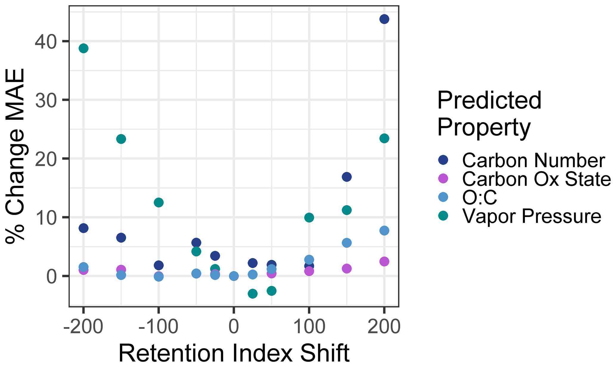
Figure 8 Percent increases in the mean absolute error in chemical property prediction as a function of the shift in a test set retention index relative to the training set retention index. Retention indices are normalized to a linear alkane series, making an increment of 100 indicate the retention time differences between two linear alkanes separated by one carbon number.

In summary, training and/or test data from multiple instruments and protocols can be combined to meet user needs, provided the following criteria are met: (1) the same ionization energy (typically 70 eV) is used, (2) the retention index or retention time drifts between instruments or protocols can be normalized to less than the difference of the elution time between two sequential linear alkanes (retention index drift of < 100), (3) similar phase columns are used (semi-standard nonpolar, standard nonpolar, etc.), (4) samples and training data are consistently either derivatized or underivatized and, if derivatized, use a consistent derivatization agent. It is also important to keep in mind that the training data must span the anticipated feature space of the use data set and that, in cases of doubt, this can be tested by adding extrapolation set compounds identified from the sample medium. For chemical properties modeling, this approach can be adapted from the GCxGC approach presented for any instrument using chromatography–electron ionization–mass spectrometry that has the capacity to yield at least unit-resolution mass spectra and for which spectra can be sufficiently deconvoluted to yield clean analyte spectra. The model structure and provided sample code are highly flexible and could be utilized to predict any property of interest that might reasonably be expected to be reflected in the combination of compound mass spectra and chromatographic retention time, although a performance evaluation is always important for ensuring that the patterns are sufficiently strong to enable accurate property prediction using Ch3MS-RF.

6 Conclusions

This work presents a new machine-learning-based method for quantifying and predicting chemical properties of novel organic compounds observed in the atmosphere. Based on a relatively small combined training and test set of ∼ 130 known compounds, we are able to predict the carbon numbers, vapor pressures, carbon oxidation states, and O : C ratios of ambient organic compounds with sufficient accuracy to usefully represent compound distributions in chemical property spaces that are important in atmospheric science. That these predictions are generated solely from retention indices and unit mass resolution mass spectra marks a significant step forward in the ability to characterize the novel organic components of Earth's atmosphere based on measurements generated from a wide range of commonly available atmospheric instrumentation. In GCxGC-MS applications, these methods contribute significant improvements in both accuracy and analytical efficiency for novel compound quantification that enable users to perform untargeted analysis of the rich complexity of data generated by advances in instrumentation. While the untargeted analysis data science techniques described in this work have been developed for and tested on atmospheric applications, they are not structurally limited in scope and could be applied to a wide range of chromatographic–mass spectral data sets to enable the characterization of complex organic mixtures. The open-source R script published in the Supplement is intended to provide a framework for groups throughout the atmospheric chemistry community to efficiently apply and adapt these methods to broadly enhance our ability to take advantage of the increasingly complex information provided by ever-accelerating advances in environmental chemistry instrumentation.

Appendix A

Figure A1 Mass spectrum of hexadecane, as measured by GCxGC-MS and featurized in Table A2.

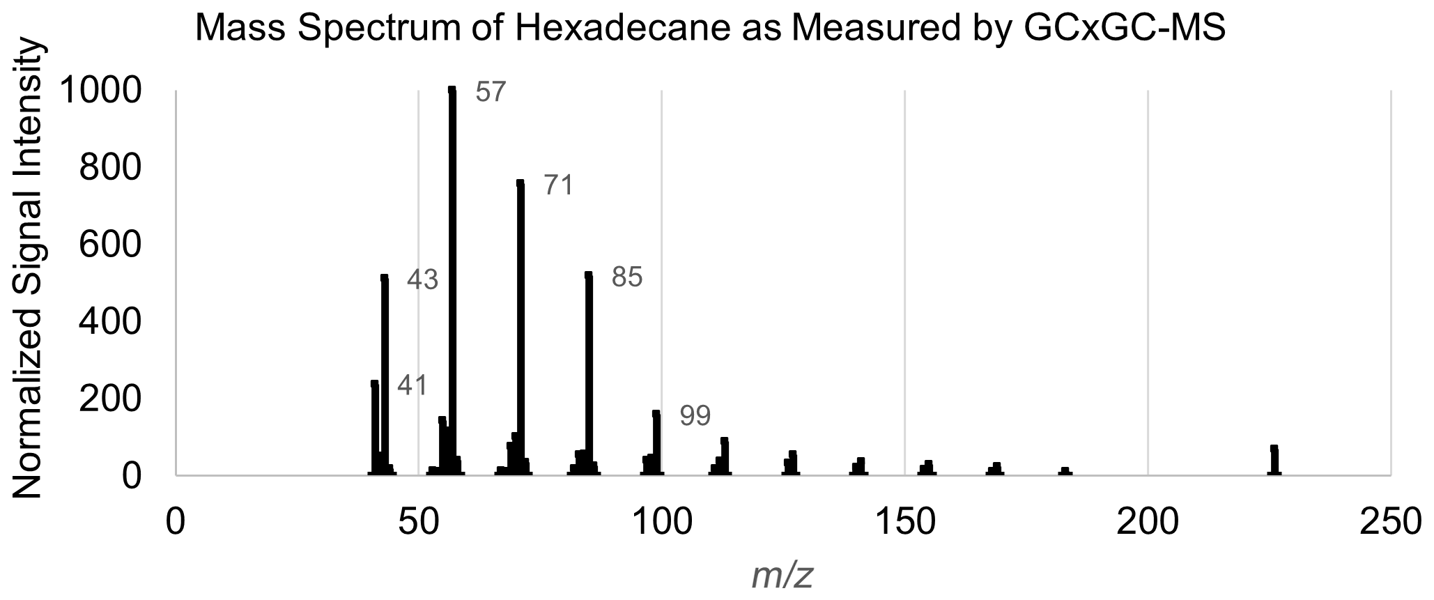
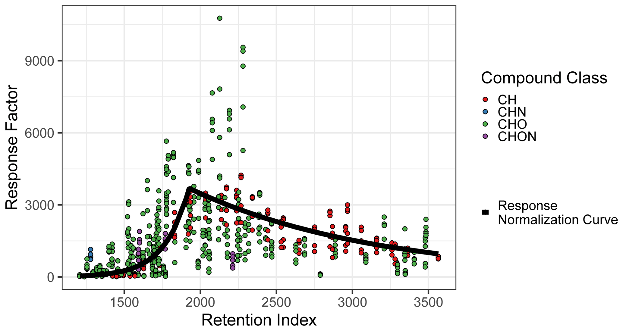
Figure A2 Quantification factor normalization curve, based on the average response factors of alkanes.

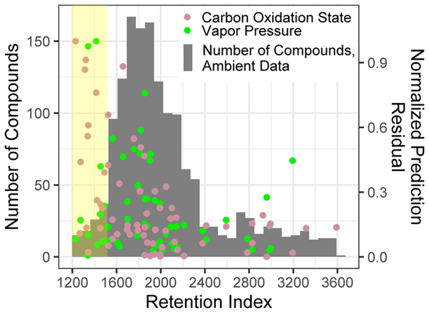
Figure A3 Normalized prediction residuals of the carbon oxidation state and vapor pressure vs. retention index for the ambient data compound property predictions set, overlaid with a compound number distribution over the retention index for ambient data set. The yellow highlighted region indicates compounds below a retention index of 1500.

Figure A4 Quantification factor prediction errors expressed in log(predicted quantification factor/true quantification factor) for test set quantification factors predicted by the random forest model (orange), closest proxy, and manual proxy methods.

Table A1 External standard names, formulae (underivatized), retention indexes, split (training set versus test set), and manually assigned quantification proxies.​​​​​​​

^a Normalized by deuterated alkane standard series. ^b Isomer identity is undetermined; only the quantification factor and properties related to chemical formula are included in modeling.

Table A2 The 40 most common charged fragments featurized for mass spectral featurization, with possible formulae and implications of published peaks.

Table A3 The 20 most common neutral mass differences between charged peaks, selected for mass spectral featurization, with possible formulae and implications of commonly reported neutral losses.

Table A4 Full chemical properties modeling features for Hexadecane.