the Creative Commons Attribution 4.0 License.
the Creative Commons Attribution 4.0 License.
 | 08 Jul 2022
A study on the performance of low-cost sensors for source apportionment at an urban background site
Dimitrios Bousiotis
David C. S. Beddows
Ajit Singh
Molly Haugen
Sebastián Diez
Pete M. Edwards
Adam Boies
Roy M. Harrison
Francis D. Pope
Knowledge of air pollution sources is important in policymaking and air pollution mitigation. Until recently, source apportion analyses were limited and only possible with the use of expensive regulatory-grade instruments. In the present study we applied a two-step positive matrix factorisation (PMF) receptor analysis at a background site in Birmingham, UK using data acquired by low-cost sensors (LCSs). The application of PMF allowed for the identification of the sources that affect the local air quality, clearly separating different sources of particulate matter (PM) pollution. Furthermore, the method allowed for the contribution of different air pollution sources to the overall air quality at the site to be estimated, thereby providing pollution source apportionment. The use of data from regulatory-grade (RG) instruments further confirmed the reliability of the results, as well as further clarifying the particulate matter composition and origin. Compared with the results from a previous analysis, in which a k-means clustering algorithm was used, a good consistency between the k means and PMF results was found in pinpointing and separating the sources of pollution that affect the site. The potential and limitations of each method when used with low-cost sensor data are highlighted. The analysis presented in this study paves the way for more extensive use of LCSs for atmospheric applications, receptor modelling and source apportionment. Here, we present the infrastructure for understanding the factors that affect air quality at a significantly lower cost than previously possible. This should provide new opportunities for regulatory and indicative monitoring for both scientific and industrial applications.
- Article
(5878 KB) - Full-text XML
- Companion paper
-
Supplement
(800 KB) - BibTeX
- EndNote


Air pollution is a major problem not only affecting human health (Pascal et al., 2013; Rivas et al., 2021; Shiraiwa et al., 2017; Wu et al., 2016; Zeger et al., 2008), but also causing environmental deterioration and social disparity due to its effect on climate change (Manisalidis et al., 2020; Mannucci and Franchini, 2017; Moore, 2009). Air pollution is typically more problematic in urban environments which have multiple air pollution sources or locations near pollution hot spots (Valavanidis et al., 2008, Bousiotis et al., 2021a). The knowledge of air pollution sources is vital in understanding the air quality at a given site as well as for policymaking and action to improve air quality. Such knowledge was provided, until recently, by the analysis of data from expensive regulatory-grade (RG) instruments. The use of RG instruments was not extensive due to their high cost and bulky size, limiting their use almost exclusively to scientific research. As a result, there is limited knowledge of the sources that affect air quality. This is in part due to the small number of deployments and hence low spatial resolution of these expensive instruments (Kanaroglou et al., 2005), especially in low- and middle-income countries. In these areas, the problem of air quality and its effect on human health is of great importance and expected to further increase in the coming years as a result of their rapid industrial and population growth (Kan et al., 2009; Petkova et al., 2013). To combat this, in the past decade, the development of low-cost sensors (LCSs) measuring either PM or gas-phase pollutant concentrations has intensified (Lewis et al., 2018; Penza, 2019; Popoola et al., 2018). These LCSs are still far from being an equal alternative to the more expensive RG instruments. Many limitations are associated with their use, with the main shortcoming being the inconsistency of their measurements, even for similar sensors deployed at the same site (Austin et al., 2015; Sousan et al., 2016), either due to operational and detector sacrifices that allow them to be inexpensive or to the effect of meteorological conditions that affect their measurements (Crilley et al., 2020; Hagan and Kroll, 2020; Wang et al., 2021). Thus, consistent calibration (Kosmopoulos et al., 2020; De Vito et al., 2020) and data corrections (Crilley et al., 2018; Liang et al., 2021; Vajs et al., 2021) are required for these sensors to provide reliable measurements, although sometimes even this is not enough (Giordano et al., 2021). Nevertheless, these sensors have the potential to change the state of air pollution monitoring by allowing for wider use and better spatio-temporal coverage.
Many applications of LCSs have been found in recent years at sites that were previously inaccessible by regulatory instrumentation, either due to them being cost-prohibitive (Miskell et al., 2018; Omokungbe et al., 2020; Pope et al., 2018) or due to their physical size limitations (Jovašević-Stojanović et al., 2015; Nagendra et al., 2019, Whitty et al., 2022). Additionally, the use of LCSs made higher spatial resolution measurements than RG instruments possible (Feinberg et al., 2019; Krause et al., 2019; Prakash et al., 2021), thereby greatly improving the ability to measure air quality at multiple locations of interest, even down to the neighbourhood scale (Schneider et al., 2017; Shafran-Nathan et al., 2019; Shindler, 2021). LCSs have been shown to help supplement existing regulatory networks (Weissert et al., 2020). While the applications of LCSs provided the information of the level of air quality at more sites, vital information on air pollution sources and the environmental conditions that enable or inhibit air pollution, as well as their relative contributions, is yet to be exploited by LCS data. Pope et al. (2018), using PM ratios, managed to separate and identify the effect of major sources of pollution in several cities in East Africa LCS data. Popoola et al. (2018) identified the sources of pollution near Heathrow Airport, London, using a network of LCSs. Bousiotis et al. (2021b), using k-means clustering on PM data from both a LCS and an RG instrument, showed the strengths and limitations of the sensor in measuring particle number concentrations and used them to identify the sources of pollution at a background site in Birmingham, UK. While these studies identified many sources and conditions that affect air quality, they provided no information on their temporal variability and the relative contributions of different sources.
In the present study, a two-step PMF technique proposed by Beddows and Harrison (2019), an advanced version of a statistical method for source apportionment successfully applied in many studies with RG instruments (Beddows et al., 2015; Harrison et al., 2011; Hopke, 2016; Leoni et al., 2018; Pokorná et al., 2016), is applied on data collected from various LCSs. This provides a quantitative separation of the different sources and their contributions to a background site located in Birmingham. Furthermore, data from RG instruments and an aerosol chemical speciation monitor (ACSM) were used to provide further nuance to the analysis. This was done not only to compare the results from the two sets, but to further characterise the sources of larger-sized particles at the site as well. The results of the present analysis are also compared with those from a previous study at the same site made by Bousiotis et al. (2021b) using k-means clustering, displaying the additional information provided by the PMF as well as checking the consistency of the results between the two methods. To the authors' knowledge, source apportionment with LCS data has only been attempted previously by Hagan et al. (2019) using non-negative matrix factorisation (a derivative version of PMF in which all components of the data matrix are weighted equally rather than with individual errors) on a dataset from New Delhi, India. This study provided information about combustion and non-combustion air pollution sources as well as their partial contributions in a three-factor solution. The present work prepares the ground for future use of source apportionment with LCSs in a variety of scientific and industrial scenarios. This will make their wider use more feasible, either as stand-alone air pollution data sources or in combination with RG instruments for increasing spatial coverage.
2.1 Location of the site and instruments
The measurement site is the Birmingham Air Quality Supersite (BAQS), located at the grounds of the University of Birmingham (52.45∘ N, 1.93∘ W) (Fig. 1). This is an urban background site within a large residential area about 3 km southwest of the city centre of Birmingham. For this site, PM concentration measurements in the range 0.35 to 40 µm were collected using an Alphasense OPC-N3 in a 10 s resolution (averaged in 1 h resolution) for the period between 16 and 30 October 2020. Additionally, data from several LCSs were also collected. NO, NO2 and ozone measurements were collected using the Box Of Clustered Sensors (BOCS; Smith et al., 2019) in the same time resolution, as well as black carbon (BC) concentrations using the MA200 sensor by Magee Scientific. Finally, the data for the lung-deposited surface area (LDSA) of particles in the range of 10 nm to 10 µm, which is found to strongly correlate with BC emissions (Lepistö et al., 2022), were collected using a set of two Naneos Partectors by Naneos Particle Solutions GmbH. One sensor measured the surface of all particles in this size range, while the second is placed after a catalytic stripper (Catalytic Instruments CS015) which removes the semi-volatile particles (Haugen et al., 2022).
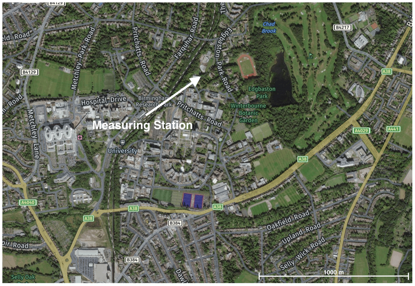
Figure 1Map of the measuring station. Imagery @2022 Bluesky, Getmapping plc, Infoterra Ltd & Bluesky, Maxar Technologies, The GeoInformation Group, map data © 2022.
Apart from the data provided directly from the sensor before the catalytic stripper, the ratio between the measurements of the two Naneos Partectors was also considered according to
This was done to resolve whether such a configuration can provide additional information for the origin of pollution or the age of the pollutants in the incoming air masses, as increased concentrations of semi-volatile compounds are usually associated with anthropogenic sources, especially in the urban environment (Mahbub et al., 2011; Schnelle-Kreis et al., 2007; Xu and Zhang, 2011). Thus, a high LDSAratio is expected to be associated with fresher pollution, which usually has a higher content of volatile compounds (i.e. pollution sources at a close distance from the site), while lower ratios are probably associated with either cleaner conditions or more regional and aged pollution, with higher concentrations of semi-volatile compounds, generally associated with sources at a greater distance from the measuring site. This specific metric was also used in our previous study (Bousiotis et al., 2021b), and the consistency of the results between the two will be compared.
For better characterisation of the larger particles, the Aerodyne ACSM was used, providing information about its composition in the size range between 40 nm and 1 µm for NO, SO and organic content. For the comparison of the results, data from RG instruments were also used, namely a Palas FIDAS (for PM), a Teledyne T500U (for NOx), a Thermo 49i (for O3) and an AE33 aethalometer from Magee Scientific (for BC). Comparison of the regulatory instruments and the LCS allows consistency of the results between instrument types to be checked. A detailed description of the operation and more information about the sensors and instruments used in this study can be found in Bousiotis et al. (2021b).
2.2 Positive matrix factorisation and data analysis
The PMF is a multivariate data analysis, developed by Paatero and Tapper (1993, 1994), which is the most commonly used method for source apportionment and has been applied numerous times in the field of aerosol science. The method is a weighted least-squares technique that describes relationships among species measurements (Reff et al., 2007). It assumes that X is a matrix of observed data, typically either particle number size distributions (PNSDs) or chemical composition data, and u is the known matrix of the experimental uncertainty of X. Both X and u are of dimensions n×m (where n is the number of measurements, and m is the number of species measured). The method solves the bilinear matrix problem , where F is the unknown right-hand factor matrix (sources) of dimensions p×m, G is the unknown left-hand factor matrix (contributions) of dimensions n×p and E is the matrix of residuals. The problem is solved in the weighted least-squares sense: G and F are determined so that the Euclidean norm of E divided (element by element) by u is minimised. Furthermore, the solution is constrained so that all the elements of G and F are required to be non-negative (Paatero and Tapper, 1994). Higher F values account for better association of the given variable with the factor it is assigned to, while higher G values account for greater contribution of the factor at the given time period.
In the present analysis, a combination of both PNSD and particle composition data was used. Such a combination may cause several shortcomings in the application of the PMF as different types of data are used, due to the significant difference between the nature of each variable. While this could be overcome by increasing the total weights of the primary group of measurements (the one considered better in driving the model), this could be problematic in the treatment and importance of the auxiliary dataset in the model (Beddows and Harrison, 2019). To overcome these shortcomings, the two-step PMF method, proposed by Beddows and Harrison (2019), was used. In the first step of the method, a part of the dataset is PMF-analysed (i.e. composition), and a solution is provided. The time series G values (and errors) of the solution from the first step are then used as input variables to the second step, where they are combined with the dataset of additional measurements (i.e. PNSD data), applying a second PMF analysis (a flow diagram of the method used as presented by Beddows and Harrison, 2019, is found in Fig. S1 in the Supplement). In the present study, the opposite path was considered, with the first step using the PNSD provided by the OPC sensor and the inclusion of particle composition data in the second step. This was explicitly done for two reasons: (1) to test the capabilities of the LCS in source apportionment and (2) to connect specific PNSD profiles with specific pollution sources. Furthermore, in the second step of the analysis detailed in Beddows and Harrison (2019), the explained variance of the factors from the first step was maximised. This directly connects the additional variables in the second step with the PNSD profiles found in the first step, excluding the possible factors formed with the data from the additional LCS data. In the present study, this step in this method was omitted, as the aim is to present the results of the receptor model as they occur in real life using a combination of LCSs measuring both particle number concentrations and composition.
As PMF is a descriptive model, there is no objective criterion in the choice of the optimal number of factors (Paatero et al., 2002). In all cases, several solutions were tested, and the solution chosen was the one that provided factors with unique properties. Solutions with additional factors provided no extra information on additional sources; rather the additional factors separated factors that had already been found into smaller groups with no significant covariation.
For the study site, particle number concentration data were available from the OPC for particles of diameter <40 µm, but only data up to 10 µm were used. This was due to the lack of sufficient non-zero counts in the larger-sized bins above that size threshold, which disfavours PMF analysis from being completed. Additionally, separate LCS data for NO and NO2 were available from the BOCS. The NO data showed sensible variation (which is the more important factor in the PMF analysis); however, a great number of the NO data points had low negative values due to their very low concentrations, which is impossible data for the PMF algorithm. Rather than removing the negative numbers or artificially calibrating the data upwards, we use NOx (NO + NO2) as the variable of interest.
Finally, to avoid the increased uncertainties from the use of unavailable data (as missing data are treated with increased uncertainties), a time window for which all data were available was chosen. Thus, data availability is 100 %, and no special treatment was considered for missing data.
Finally, for the present study the PMF analysis was performed using the second iteration of the PMF software developed by Paatero (2004a, b). Data were analysed using the Openair package for R (Carslaw and Ropkins, 2012), and back trajectory data were extracted by NOAA Air Resources Laboratory and calculated using the HYSPLIT model (Draxler and Hess, 1998).
3.1 General conditions at the BAQS site and overall performance of the low-cost sensors
The measuring period (16 to 30 October 2020) was chosen as it is a period which presented rather typical meteorological conditions in the area and had no missing data from any of the instruments used and because they were the last days before the second lockdown due to COVID-19 was applied (31 October 2020). General meteorological conditions were rather typical for the period in Birmingham, UK. As a result, the conditions and activities in the surrounding area found in this period are considered almost consistent with the normal conditions at the site in the autumn season. Mean temperature was 10.0±2.5 ∘C, and mean relative humidity was 87.9±7.5 % (standard deviations are calculated using hourly data) during the measurement period. The average wind profile (Fig. S2) was also typical for the UK, with mainly southwestern winds of relatively low speed (2.1±1.1 m s−1).
Most of the LCSs correlated well when compared to their more expensive RG counterparts, using the Pearson correlation coefficient as the measure of correlation. The OPC-N3 presented a strong correlation for PM1 (r=0.88), though its performance weakened with greater-sized PM (r=0.49 for PM2.5 and r=0.46 for PM10). The decreasing correlation from PM1 to PM2.5 to PM10 is likely due to greater wall losses in the tubing for the bigger particles. Strong correlations were also found from the BOCS as well, with both O3 and NOx concentrations presenting high r values when compared with their respective RG instrument measurements (0.95 and 0.82 respectively). Finally, the BC-measuring LCS presented lower agreement with the measurements from the RG instrument, with a Pearson correlation value of 0.40. It is noted that in the present study the absolute performance of the LCS is not of great importance, and thus it is not analysed in depth. For the PMF model to present meaningful results, the representation of the relative values and variability of the variables is crucial instead, and this is thoroughly tested in the present study.
3.2 First step PMF analysis (PNSD analysis)
Following the discussed methodology, a four-factor solution was chosen for this analysis. The PNSD profiles of the factors found are presented in Fig. S3. Due to the limited variation of the PNSD profiles when presenting all the size bins available, making some of them appear identical (i.e. Factors 2 and 3, due to the increasing particle number concentration as the size decreases), the smallest particle diameter size bin at 400 nm (particle diameter range between 350 and 460 nm) was removed to better present the variation on the larger sizes. Thus, the particle profiles without the smallest available size are presented in Fig. 2. The profiles in the range between 500 nm and 10 µm for the four factors, associated with unique formations extracted from the method, are as follows:
-
Factor 1, that presents no significant peaks in the measured range of the OPC but does show a steady increasing trend with particle diameters below 1 µm;
-
Factor 2, with a distinct particle diameter peak at about 2 µm;
-
Factor 3, with a distinct particle diameter peak at about 2 µm and an increasing trend below 750 nm;
-
Factor 4, accounting for particle diameter peaking at about 750 nm and 1.5 µm.
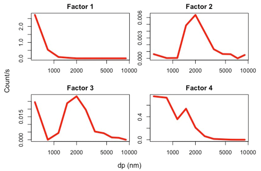
Figure 2Particle profiles of the factors from the PMF analysis (above 500 nm). The lines indicate the average particle count per second for each particle size bin.
3.3 Second-step PMF with LCS data (LC analysis)
The four-factor solution was also chosen in the second-step analysis, for which the results of the first step are combined with the additional particle- and gas-phase composition datasets from LCSs. The addition of more factors instead of adding information or providing clearer associations with the factors from the first step separated the existing factors and their association with the particle composition data into mixed factor groups with less significant contributions of the variables. The association of the variables with each factor is presented in Fig. 3, while the temporal variation of the contributions G of all the factors from this analysis is presented in Fig. 4, along with the wind profile for some periods when each factor was dominant.

Figure 3Contribution of the factors from the LC analysis. Grey bars indicate the values of F, while red bars indicate the explained variations for each variable.
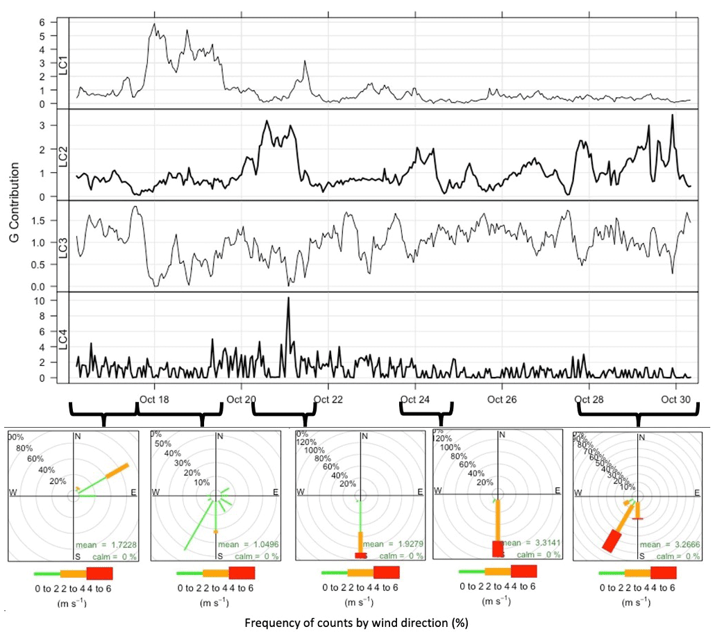
Figure 4Temporal variation of the contributions of the factors from the LC analysis. The wind roses refer to the wind conditions for the corresponding periods when specific factors presented higher G contributions.
The four new factors are as follows:
-
LC1 (local and city centre pollution on calm conditions). The LC1 is strongly associated with the first factor from the initial PMF on the PNSD. For the period when the contribution of this factor is higher (18 and 19 October; see Fig. 4), rather slow winds prevail from many sectors (in this case mainly from the southwest). This factor has higher contributions during calm conditions and during periods with northeastern winds, though with lower contribution (Fig. 5). It is highlighted that northeast of the specific site is the city centre of Birmingham, which is one of the main sources of pollution, as found from a previous study (Bousiotis et al., 2021b). Looking at the diurnal variation (Fig. S4) of this factor, we see increased contributions during early morning and evening hours, likely associating it with the morning and evening rush hours. The increased contributions during night-time should not be overlooked and are probably the result of the lower boundary layer height (BLH) during this time of the day. Additional data analysis shows an increased association of this factor with PM1 (Fig. 3), though this association is reduced for particles of larger sizes, further confirming the lack of additional peaks on greater sizes. This along with the increased association with the LDSA indicates the presence of a large number of particles below the detection limit of the instrument. This factor is also associated with almost all the pollutants used, such as NOx, CO and BC, though not as strongly as factor LC3 that is discussed below, probably associated with pollution sources in a closer range to the measuring station, as well as to a smaller extent with pollution from the city centre. Its connection with air masses from the northeast is also confirmed from the back trajectory analysis (Fig. 6), in which the highest contributions of this factor were found for air masses from the northeast.
-
LC2 (marine). This factor is strongly associated with the fourth PNSD factor from the initial analysis (Fig. 3). It presents relatively high association with PM, which increases as the size increases. No other significant association is found rather than relatively weak ones with ozone, CO and the LDSAratio. It does not have a clear diurnal variation (Fig. S4), though it has slightly increased contributions during night-time. Higher contributions for this factor are found with south and southeastern winds of high speed (Figs. 4 and 5). This can be seen in Fig. 4, where the highest contributions of this factor are associated with strong southern winds. The marine nature of this factor is clearly highlighted through the back trajectory analysis for this factor (Fig. 6) in which higher contributions are mostly found with air masses originating from the north Atlantic Ocean, while some contributions are from southern Spain and Africa, which may be associated with Saharan dust and pollution from these areas.
-
LC3 (midday city centre and southwestern pollution). This factor does not have any significant association with any of the factors from the PMF analysis of the PNSD (Fig. 3). It presents greater contributions during the midday (Fig. S4), and it is associated with northeastern and southwestern winds (Fig. 5). It has high contributions with all the pollutants included in the analysis and the LDSAratio, which points to fresher pollution (pollution sources closer to the measuring station). Such sources of pollution in most cases are associated with particles of sizes smaller than that measured by the OPC, hence the lack of association with any of the factors found from the PNSD analysis. The back trajectory analysis provides no clear origin for the air masses of this factor (Fig. 6), which may indicate a relatively smaller pollution lifetime, which is associated with incoming air masses from all directions.
-
LC4 (urban background). This factor has a rather strong association with the second factor from the PNSD analysis and a weaker one with the third one (Fig. 3). It does not have a clear diurnal variation (Fig. S4), and it is mainly associated with northeastern winds (Fig. 5). It presents weak associations with all the variables inputted in the PMF analysis, making it hard to distinguish either a source or conditions for which this factor is enhanced. The back trajectory analysis though shows that this factor is associated with air masses from continental Europe as well as Scandinavia (Fig. 6), which for the UK, usually contain aged and hence typically larger secondary PM pollutants.
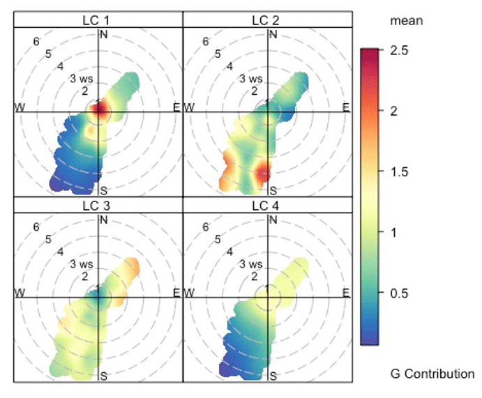

Figure 6Average G contribution of the factors from the LC analysis for incoming air masses. Higher contributions indicate better association of the given factor with the corresponding air mass origin.
3.4 Second-step PMF with RG data (RG analysis)
While the primary aim of the present study is to highlight the capabilities of LCSs in source apportionment, the measurements provided by these devices are mainly focused on gas-phase pollutants which are in most cases associated solely with ultrafine particles. The OPC measurements used for this site have a particle diameter range between 400 nm and 10 µm. Thus, apart from using data from RG instruments measuring gas-phase pollutants, it was considered sensible to add data from an ACSM, which measures compounds associated with larger particles, such as nitrate, sulfate and organic compounds (used in this analysis).
Some of the factors in this analysis are rather similar with those formed from the analysis using the LCS dataset. Thus, the RG1 factor in this analysis is mainly associated with the first factor from the PNSD analysis in the first step (Fig. 7), similar to that found also in LC1 (Fig. 3). The wind conditions are also similar for which these factors from the two analyses present their highest contribution (Fig. 8), as well as their temporal variation (Fig. S5) and diurnal variation (Fig. S6). The additional information granted using the ACSM data is the strong association of this factor with nitrate, and a stronger association with NOx and BC is also found, compared to the LC analysis. This further associates this factor with nearby sources of pollution which prevail with low wind speeds and may associate the conditions of this factor with the low BLH height found during that time, though high contributions were also found for early morning and evening hours, as in the LC analysis for the similar factor. Finally, the back trajectory analysis (Fig. 9) shows higher contributions associated with air masses from the northeast, further confirming its similarity with the first factor from the LC analysis and its urban origins.
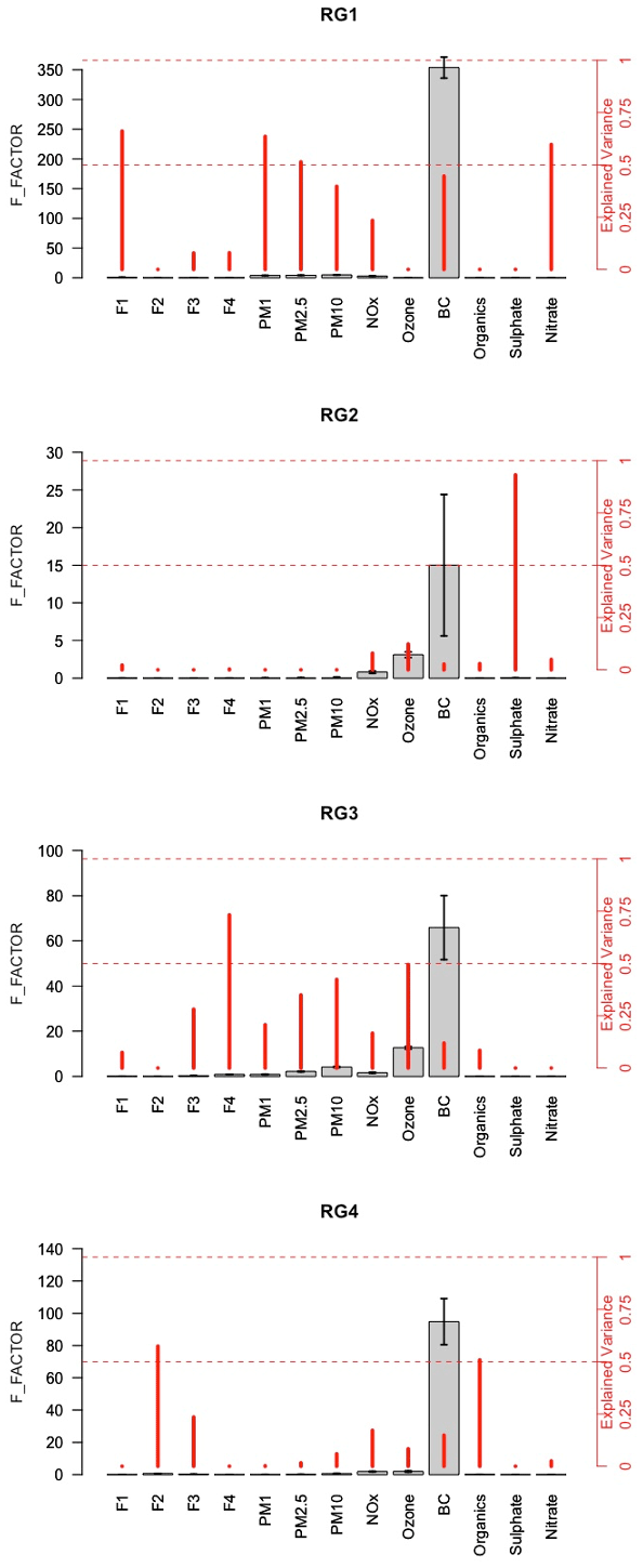
Figure 7Variable association for the factors from the RG analysis. Grey bars indicate the values of F, while red bars indicate the explained variations for each variable.

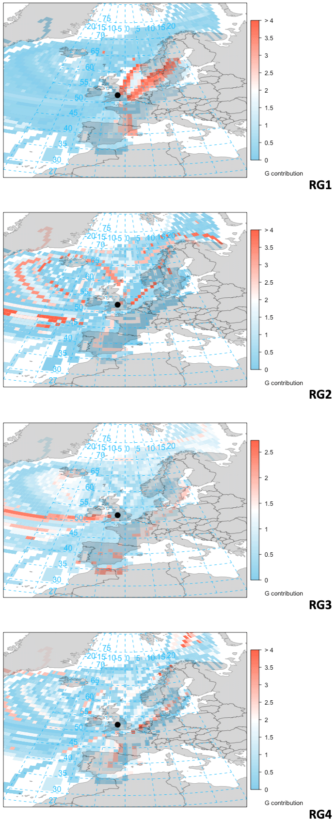
Figure 9Average G contribution of the factors from the RG analysis for incoming air masses. Higher contributions indicate better association of the given factor with the corresponding air mass origin.
The RG2 is unique and has no association with the factors from the PMF on PNSD data and is strongly associated only with sulfate (Fig. 7). It does not have a clear diurnal variation (Fig. S6) and seems to have higher contributions with southwestern winds of rather high speed and to a lesser extent with northeasterly winds (Fig. 8). The back trajectory analysis (Fig. 9), while presenting few relatively high contributions from continental Europe, mainly associates this factor with incoming air masses from all sea origins surrounding the UK. This is expected as the ocean is a source of sulfate-containing compounds (for the particles at the size range measured by the OPC), either sea-salt sulfate or marine biogenic sulfate (Lin et al., 2012; Raes et al., 2000).
The RG3 is similar to the LC2 and is mainly associated with the fourth factor from the PNSD analysis and to a lesser extent with the third (Fig. 7). This factor has slightly increased contributions during night-time (Fig. S6) and south and southwestern winds (Fig. 8). It presents increased associations with increasing PM size, though in this case it is also strongly associated with O3. Unfortunately, no Cl or Na data were available to further determine the marine nature of this factor. The back trajectory analysis though once again presents higher contributions with marine air masses (Fig. 9), though some hot spots are also found from continental Europe, which probably explain to an extent the small associations found with NOx and organic compounds from the ACSM.
Finally, the RG4 is mainly associated with the second factor and to a lesser extent with the third from the PNSD analysis (Fig. 7). It presents higher contributions with northeastern winds (Fig. 8), has an unclear diurnal variation (Fig. S6) and presents higher contributions with air masses from continental Europe (Fig. 9), like the LC4 from the second-step analysis. While in that analysis it was difficult to characterise the sources for that factor, the strong association with organic compounds found here with the addition of the ACSM data helps in its clearer characterisation.
4.1 Comparison of the results from the second-step analysis
It should be noted that regardless of any possible similarities between the two (second-step) analyses, a direct comparison of the results should be conducted with great care. As different variables are considered, even minor differences may result in different trends, contribution of variables and the sources described. Regardless, the results of the two analyses have great similarities, especially for specific factors that are associated with the same particle size distribution profiles (from the PNSD analysis), contribution of chemical compounds and diurnal variation. Three factors were found to have great similarities and were associated with similar particle profiles. Specifically, these are the factors describing the sources of particles which are either in close proximity to the measuring station or occur with almost calm conditions (Factor 1 on both analyses), the marine factor (Factor 2 on LC analysis and Factor 3 on RG analysis) and the continental factor (Factor 4 on both analyses). Looking at their temporal contributions (Figs. 4 and S5), the first factors on both analyses appear to consistently peak in periods when the second set of factors (LC2 and RG3) presents lower G contributions (and vice versa), which is expected due to the nature of their sources. The factors on both sets though have almost identical temporal variation of their G contributions, regardless of the dataset. For the fourth factors on both analyses, though presenting similar associations with their variables, differences are found in their temporal variations with the addition of the ACSM data. This shows that while these factors appear to be almost identical, small differences can still be found in their temporal variation and variable associations, when different datasets are considered. Nevertheless, the addition of the ACSM data shows a very high contribution of NO in the first RG factor, SO in the second factor and the organic component in the fourth factor.
The remaining factor from both analyses though is completely different between the two analyses and points towards the differences on the variables used for each. In the LC analysis, the factor formed consists of sources that are associated with fresher pollution sources. Thus, a factor with strong associations with all the pollutants available was formed; it was not associated with any of the PNSD formations from the first-step analysis and presented a unique diurnal variation peaking midday. This should be expected as the particle size measured by the OPC is much larger compared to the size of the particles these chemical compounds are usually associated with. The occurrence of this factor was probably included partially to the first and fourth factor of the RG analysis, as these present relatively higher associations with NOx and BC and more enhanced contributions during midday hours compared to their LC analysis counterparts.
Finally, using the RG instrument data, the additional factor is associated with sulfate alone. This is a result that was consistent, regardless of the number of factors used, either greater or smaller. Sulfate-containing compounds have a lower volatility compared to the other chemical compounds used in the analysis and are relatively more stable with a rather small seasonal variation (Utsunomiya and Wakamatsu, 1996), thus having a longer lifespan and distance of travel. As a result, sulfate was found not to be associated with any other chemical compound and always formed a factor of its own (regardless of the number of factors chosen).
4.2 Comparison with the results from a previous study
Although different methodologies were used with the previous analysis for the BAQS site (Bousiotis et al., 2021b), as well as for different time periods, many similarities were found for the sources of particles at the site. The main source of smaller particles at the site in the previous analysis is found to be the city centre in the northeast, for which relatively high concentrations of NOx were found. Similar is the case in the present analysis, as for the sources found to be associated with northeasterly winds, an association was also found with NOx and the LDSAratio. Additionally, a source of sulfate found with southerly winds was also confirmed in the present study, with the association of high sulfate concentrations with a factor which presents higher contributions with winds from the southern sector. While in the previous analysis the sources responsible for this source could not be pinpointed, in the present analysis, using a back trajectory analysis, the sulfate factor was associated with marine particle sources from all directions. Furthermore, a factor in the present analysis, which identifies hot spots south of the measuring station with strong presence of PM of all sizes, was also found with the k-means analysis in the previous study, though in that case it was more associated with the pollution sources from that side rather than the long-range transport found here.
These similarities are very encouraging, as even though the analyses were made for different periods and using different methods, there is consistency between the results. This means that regardless of the different seasons studied (previous analysis was performed during winter to early spring), the sources of particles (and pollution) are relatively uniform, without significant changes.
Additionally, the k-means method identified sets of conditions that either promote or suppress the pollution at the sites (as this can be illustrated with the variable particle concentrations between the clusters found from the analysis), rather than separate sources of pollution that affect the site. While this provides a more realistic picture of the conditions, it makes it harder to distinguish the specific sources and their effect in its air quality. On the other hand, the PMF not only provides clearer separation of the sources, but the temporal contribution of each source as well, which shows the real extent of the effect of each source of particles or pollutants, thus achieving source apportionment rather than just the identification of pollution sources that the k means offers. The k-means approach identifies the effect of the sources of particles, but it also separates cleaner periods as separate clusters. These two effects gives a more complete overall picture of the air quality at a site. PMF could also provide this information, but it would be more difficult to obtain looking at the different sources and the conditions that keep them as low contributions (this would also require a much greater number of factors).
Furthermore, due to the complexity of the clusters from the k means, pinpointing the sources that the particles are associated with is difficult. This is due to the clusters, being a set of different sources and conditions rather than clearly separated sources, not being clearly associated with distinct wind directions, speeds or hot spots. Contrary to that, the factors formed by the PMF present clearer association with specific sectors, thus making it easier to define the sources associated with them, as in the results they are presented as hot spots within the polar plots.
The analysis of atmospheric data using either k means or PMF is proven to provide adequate and trustworthy information for the sources of particles and by extension of pollution at a site, even with the sole use of LCSs, as shown in this paper and the preceding Bousiotis et al. (2021b) paper. The combined use of both approaches provides a clearer picture of the different sources and their effect, as the PMF is able to better separate and provide the effect of the sources of pollution that affect the air quality at a site, and the k means provides a more realistic representation of the conditions at a site, by showing the combined effect of these sources. The relative consistency of the results found between the two analyses, even being in different time periods, is very encouraging and shows that the very important information of pollution receptor modelling is viable with LCSs, providing a much needed alternative for countries or scenarios where the use of regulatory-grade instruments is not feasible. The significantly lower price point of LCSs means that in addition to hyperlocal measurement of air pollution, it should now be possible to deliver hyperlocal source apportionment of air pollution, though as highlighted within this study, there are some limitations for specific sources associated with pollutants with certain properties. Further exploration of these limitations and design of methodologies to overcome them can enhance their capability and open new research and industrial abilities to pinpoint air pollution sources and subsequently manage them.
Finally, the LDSAratio, a variable that was introduced in the previous analysis, was included in the present one as well. As in the previous analysis, this ratio was found to be more associated with fresher pollution from combustion sources near to the measuring station, for which it has reliably performed in both analyses.
To solve air quality problems and to deliver the associated policymaking effectively, it is vital to have a methodology to measure the sources of air pollution, and their relative importance. Historically, this has been achieved using expensive RG instruments. The cost implications of these studies make assessment at dense spatial resolutions limited. In this study, data from a low-cost OPC and other LCSs, measuring gas-phase pollutants, black carbon and the lung-deposited surface area of particles in BAQS were analysed using the two-step PMF analysis. Four factors were formed from this analysis and were associated with their respective sources and to a great extent with unique PNSD profiles. The following factors were found: a factor associated with either combustion sources in close proximity of the measurement site or calm conditions, a marine factor, a factor associated with midday activities from the city centre and a more constant factor from the northeast. The same analysis was also performed using data from RG instruments and the same PNSD factors. This was done to evaluate the results from the low-cost sensor analysis as well as to further characterise and clarify the sources associated with the factors formed. Significant agreement was found between the results of the two analyses, highlighting that the LCSs are capable of carrying out such analyses. The additional ACSM data from the second analysis further helped in the characterisation of the composition of the particles of each factor, clarifying the sources associated with nitrate, sulfate and organic compounds at the site, as well as strongly associating some with unique PNSD profiles. While in their present state, the LCSs do not possess the full capability of the RG instruments for providing high-accuracy measurements, considering the limitations they were found to be adequate in providing with the trends of the particles and pollutants measured which are important for source apportionment studies. This is done at a fraction of the equipment cost; see Bousiotis et al. (2021b) for cost estimates.
Furthermore, comparing the results from the PMF to those from the k-means analysis showed the different strengths and weaknesses of each approach. The PMF is better in pinpointing the effect of separate sources of pollution, but it is difficult to give a clear representation of the actual conditions when each factor affects the site. The k means is not as efficient in clearly separating the different sources, but it does provide a more realistic picture of the air quality at a site in relation to the ambient conditions. The combined use of both methods though provided a clearer picture for the conditions at the site.
The methodologies developed and used in this study will help to reliably facilitate source apportionment studies in the future, with either the sole use of LCSs or their combination with RG instruments. As for a given site, specific PNSD formations are associated with specific conditions and sources (Harrison et al., 2011), by creating a repository of unique PNSDs at a site and associating them with their respective sources; in the future the source apportionment may be done to an extent using only PNSD profiles and meteorological data alone. This will do much in simplifying the source apportionment process, allowing for its wider application and helping in dealing with environmental challenges, though it can be challenging in sites with particle emissions smaller than what the OPC can measure (e.g. vehicle exhaust emissions). For this though, further testing in more diverse environments and scenarios is needed, which, along with the anticipated development of the LCS, will provide a denser and reliable measuring network, even for countries with lower incomes, and help reach cleaner and healthier environmental conditions.
The code for the PMF2 used in the data analysis of this study is a proprietary piece of software licenced by Pentti Paatero and thus cannot be shared without the author’s permission.
Data supporting this publication are openly available from the UBIRA eData repository at https://doi.org/10.25500/edata.bham.00000856 (Pope and Bousiotis, 2022).
The supplement related to this article is available online at: https://doi.org/10.5194/amt-15-4047-2022-supplement.
The study was conceived and planned by FDP, who also contributed to the final paper, and DB, who carried out the analysis and prepared the first draft. AS, MH, DCSB and SD provided data for the analysis. DCSB provided help with the analysis of the data. RMH, PME and AB contributed to the final paper.
The contact author has declared that neither they nor their co-authors have any competing interests.
Publisher's note: Copernicus Publications remains neutral with regard to jurisdictional claims in published maps and institutional affiliations.
We thank the OSCA team (Integrated Research Observation System for Clean Air) at the Birmingham Air Quality Supersite (BAQS), funded by NERC (NE/T001909/1), for help in data collection for the regulatory-grade instruments. We thank Lee Chapman for access to his meteorological dataset used in the analysis.
This research has been supported by the Natural Environment Research Council (NERC; grant no. NE/T001879/1), the Engineering and Physical Sciences Research Council (EPSRC grant no. EP/T030100/1) and internal EPSRC funding provided to the University of Birmingham for Impact Acceleration.
This paper was edited by Albert Presto and reviewed by Priyanka DeSouza and one anonymous referee.
Austin, E., Novosselov, I., Seto, E., and Yost, M. G.: Laboratory evaluation of the Shinyei PPD42NS low-cost particulate matter sensor, PLoS One, 10, 1–17, https://doi.org/10.1371/journal.pone.0137789, 2015.
Beddows, D. C. S. and Harrison, R. M.: Receptor modelling of both particle composition and size distribution from a background site in London, UK – a two-step approach, Atmos. Chem. Phys., 19, 4863–4876, https://doi.org/10.5194/acp-19-4863-2019, 2019.
Beddows, D. C. S., Harrison, R. M., Green, D. C., and Fuller, G. W.: Receptor modelling of both particle composition and size distribution from a background site in London, UK, Atmos. Chem. Phys., 15, 10107–10125, https://doi.org/10.5194/acp-15-10107-2015, 2015.
Bousiotis, D., Pope, F. D., Beddows, D. C. S., Dall'Osto, M., Massling, A., Nøjgaard, J. K., Nordstrøm, C., Niemi, J. V., Portin, H., Petäjä, T., Perez, N., Alastuey, A., Querol, X., Kouvarakis, G., Mihalopoulos, N., Vratolis, S., Eleftheriadis, K., Wiedensohler, A., Weinhold, K., Merkel, M., Tuch, T., and Harrison, R. M.: A phenomenology of new particle formation (NPF) at 13 European sites, Atmos. Chem. Phys., 21, 11905–11925, https://doi.org/10.5194/acp-21-11905-2021, 2021a.
Bousiotis, D., Singh, A., Haugen, M., Beddows, D. C. S., Diez, S., Murphy, K. L., Edwards, P. M., Boies, A., Harrison, R. M., and Pope, F. D.: Assessing the sources of particles at an urban background site using both regulatory instruments and low-cost sensors – a comparative study, Atmos. Meas. Tech., 14, 4139–4155, https://doi.org/10.5194/amt-14-4139-2021, 2021b.
Carslaw, D. C. and Ropkins, K.: openair – An R package for air quality data analysis, Environ. Modell. Softw., 27–28, 52–61, https://doi.org/10.1016/j.envsoft.2011.09.008, 2012.
Crilley, L. R., Shaw, M., Pound, R., Kramer, L. J., Price, R., Young, S., Lewis, A. C., and Pope, F. D.: Evaluation of a low-cost optical particle counter (Alphasense OPC-N2) for ambient air monitoring, Atmos. Meas. Tech., 11, 709–720, https://doi.org/10.5194/amt-11-709-2018, 2018.
Crilley, L. R., Singh, A., Kramer, L. J., Shaw, M. D., Alam, M. S., Apte, J. S., Bloss, W. J., Hildebrandt Ruiz, L., Fu, P., Fu, W., Gani, S., Gatari, M., Ilyinskaya, E., Lewis, A. C., Ng'ang'a, D., Sun, Y., Whitty, R. C. W., Yue, S., Young, S., and Pope, F. D.: Effect of aerosol composition on the performance of low-cost optical particle counter correction factors, Atmos. Meas. Tech., 13, 1181–1193, https://doi.org/10.5194/amt-13-1181-2020, 2020.
De Vito, S., Esposito, E., Castell, N., Schneider, P., and Bartonova, A.: On the robustness of field calibration for smart air quality monitors, Sensor. Actuat. B-Chem., 310, 127869, https://doi.org/10.1016/j.snb.2020.127869, 2020.
Draxler, R. R. and Hess, G. D.: An Overview of the HYSPLIT_4 Modelling System for Trajectories, Dispersion, and Deposition, Aust. Meteorol. Mag., 47, 295–308, 1998.
Feinberg, S. N., Williams, R., Hagler, G., Low, J., Smith, L., Brown, R., Garver, D., Davis, M., Morton, M., Schaefer, J., and Campbell, J.: Examining spatiotemporal variability of urban particulate matter and application of high-time resolution data from a network of low-cost air pollution sensors, Atmos. Environ., 213, 579–584, https://doi.org/10.1016/j.atmosenv.2019.06.026, 2019.
Giordano, M. R., Malings, C., Pandis, S. N., Presto, A. A., McNeill, V. F., Westervelt, D. M., Beekmann, M., and Subramanian, R.: From low-cost sensors to high-quality data: A summary of challenges and best practices for effectively calibrating low-cost particulate matter mass sensors, J. Aerosol Sci., 158, 105833, https://doi.org/10.1016/j.jaerosci.2021.105833, 2021.
Hagan, D. H. and Kroll, J. H.: Assessing the accuracy of low-cost optical particle sensors using a physics-based approach, Atmos. Meas. Tech., 13, 6343–6355, https://doi.org/10.5194/amt-13-6343-2020, 2020.
Hagan, D. H., Gani, S., Bhandari, S., Patel, K., Habib, G., Apte, J. S., Hildebrandt Ruiz, L., and Kroll, J. H.: Inferring Aerosol Sources from Low-Cost Air Quality Sensor Measurements: A Case Study in Delhi, India, Environ. Sci. Tech. Let., 6, 467–472, https://doi.org/10.1021/acs.estlett.9b00393, 2019.
Harrison, R. M., Beddows, D. C. S., and Dall'Osto, M.: PMF analysis of wide-range particle size spectra collected on a major highway, Environ. Sci. Technol., 45, 5522–5528, https://doi.org/10.1021/es2006622, 2011.
Haugen, M. J., Singh, A., Bousiotis, D., Pope, F. D., and Boies, A. M.: Demonstrating the ability to differentiate between semi-volatile and solid particle events with low-cost lung-deposited surface area and black carbon particle sensors, Atmosphere, 13, 747, https://doi.org/10.3390/atmos13050747, 2022.
Hopke, P. K.: Review of receptor modeling methods for source apportionment, J. Air Waste Manage., 66, 237–259, https://doi.org/10.1080/10962247.2016.1140693, 2016.
Jovašević-Stojanović, M., Bartonova, A., Topalović, D., Lazović, I., Pokrić, B., and Ristovski, Z.: On the use of small and cheaper sensors and devices for indicative citizen-based monitoring of respirable particulate matter, Environ. Pollut., 206, 696–704, https://doi.org/10.1016/j.envpol.2015.08.035, 2015.
Kan, H., Chen, B., and Hong, C.: Health impact of outdoor air pollution in China: Current knowledge and future research needs, Environ. Health Persp., 117, 12737, https://doi.org/10.1289/ehp.12737, 2009.
Kanaroglou, P. S., Jerrett, M., Morrison, J., Beckerman, B., Arain, M. A., Gilbert, N. L., and Brook, J. R.: Establishing an air pollution monitoring network for intra-urban population exposure assessment: A location-allocation approach, Atmos. Environ., 39, 2399–2409, https://doi.org/10.1016/j.atmosenv.2004.06.049, 2005.
Kosmopoulos, G., Salamalikis, V., Pandis, S. N., Yannopoulos, P., Bloutsos, A. A., and Kazantzidis, A.: Low-cost sensors for measuring airborne particulate matter: Field evaluation and calibration at a South-Eastern European site, Sci. Total Environ., 748, 141396, https://doi.org/10.1016/j.scitotenv.2020.141396, 2020.
Krause, A., Zhao, J., and Birmili, W.: Low-cost sensors and indoor air quality: A test study in three residential homes in Berlin, Germany, Gefahrst. Reinhalt. L., 79, 87–94, https://doi.org/10.37544/0949-8036-2019-03-49, 2019.
Leoni, C., Pokorná, P., Hovorka, J., Masiol, M., Topinka, J., Zhao, Y., Křůmal, K., Cliff, S., Mikuška, P., and Hopke, P. K.: Source apportionment of aerosol particles at a European air pollution hot spot using particle number size distributions and chemical composition, Environ. Pollut., 234, 145–154, https://doi.org/10.1016/j.envpol.2017.10.097, 2018.
Lepistö, T., Kuuluvainen, H., Lintusaari, H., Kuittinen, N., Salo, L., Helin, A., Niemi, J.V., Manninen, H.E., Timonen, H., Jalava, P., Saarikoski, S., and Rönkkö, T.: Connection between lung deposited surface area (LDSA) and black carbon (BC) concentrations in road traffic and harbour environments, Atmos. Environ., 272, 118931, https://doi.org/10.1016/j.atmosenv.2021.118931, 2022.
Lewis, A. C., von Schneidemesser, E., and Peltier, R. E.: Low-cost sensors for the measurement of atmospheric composition: overview of topic and future applications, World Meteorological Organization, Geneva, Switzerland, WMO-No. 1215, 46 pp., ISBN 978-92-63-11215-6, 2018.
Liang, Y., Wu, C., Jiang, S., Li, Y. J., Wu, D., Li, M., Cheng, P., Yang, W., Cheng, C., Li, L., Deng, T., Sun, J. Y., He, G., Liu, B., Yao, T., Wu, M., and Zhou, Z.: Field comparison of electrochemical gas sensor data correction algorithms for ambient air measurements, Sensor. Actuat. B Chem., 327, 128897, https://doi.org/10.1016/j.snb.2020.128897, 2021.
Lin, C. T., Baker, A. R., Jickells, T. D., Kelly, S., and Lesworth, T.: An assessment of the significance of sulphate sources over the Atlantic Ocean based on sulphur isotope data, Atmos. Environ., 62, 615–621, https://doi.org/10.1016/j.atmosenv.2012.08.052, 2012.
Mahbub, P., Ayoko, G. A., Goonetilleke, A., and Egodawatta, P.: Analysis of the build-up of semi and non volatile organic compounds on urban roads, Water Res., 45, 2835–2844, https://doi.org/10.1016/j.watres.2011.02.033, 2011.
Manisalidis, I., Stavropoulou, E., Stavropoulos, A., and Bezirtzoglou, E.: Environmental and Health Impacts of Air Pollution: A Review, Frontiers in Public Health, 8, 1–13, https://doi.org/10.3389/fpubh.2020.00014, 2020.
Mannucci, P. M. and Franchini, M.: Health effects of ambient air pollution in developing countries, Int. J. Environ. Res. Pu., 14, 1048, https://doi.org/10.3390/ijerph14091048, 2017.
Miskell, G., Salmond, J. A., and Williams, D. E.: Use of a handheld low-cost sensor to explore the effect of urban design features on local-scale spatial and temporal air quality variability, Sci. Total Environ., 619–620, 480–490, https://doi.org/10.1016/j.scitotenv.2017.11.024, 2018.
Moore, F. C.: Climate change and air pollution: Exploring the synergies and potential for mitigation in industrializing countries, Sustainability, 1, 43–54, https://doi.org/10.3390/su1010043, 2009.
Nagendra, S., Reddy Yasa, P., Narayana, M., Khadirnaikar, S., and Pooja Rani: Mobile monitoring of air pollution using low cost sensors to visualize spatio-temporal variation of pollutants at urban hotspots, Sustain. Cities Soc., 44, 520–535, https://doi.org/10.1016/j.scs.2018.10.006, 2019.
Omokungbe, O. R., Fawole, O. G., Owoade, O. K., Popoola, O. A. M., Jones, R. L., Olise, F. S., Ayoola, M. A., Abiodun, P. O., Toyeje, A. B., Olufemi, A. P., Sunmonu, L. A., and Abiye, O. E.: Analysis of the variability of airborne particulate matter with prevailing meteorological conditions across a semi-urban environment using a network of low-cost air quality sensors, Heliyon, 6, e04207, https://doi.org/10.1016/j.heliyon.2020.e04207, 2020.
Paatero, P.: User's guide for positive matrix factorization programs PMF2 and PMF3, Part1: tutorial, University of Helsinki, Helsinki, Finland, 2004a.
Paatero, P.: User's guide for positive matrix factorization programs PMF2 and PMF3, Part2: references. University of Helsinki, Helsinki, Finland, 2004b.
Paatero, P. and Tapper, U.: Analysis of different modes of factor analysis as least squares fit problems, Chemometr. Intell. Lab., 18, 183–194, https://doi.org/10.1016/0169-7439(93)80055-M, 1993.
Paatero, P. and Tapper, U.: Positive Matrix Factorization: A Non-negative factor model with optimal utilization of error estimates of data values, Environmetrics, 5, 111–126, 1994.
Paatero, P., Hopke, P. K., Song, X.-H., and Ramadan, Z.: Understanding and controlling rotations in factor analytic models, Chemometr. Intell. Lab., 60, 253–264, 2002.
Pascal, M., Corso, M., Chanel, O., Declercq, C., Badaloni, C., Cesaroni, G., Henschel, S., Meister, K., Haluza, D., Martin-Olmedo, P., and Medina, S.: Assessing the public health impacts of urban air pollution in 25 European cities: Results of the Aphekom project, Sci. Total Environ., 449, 390–400, https://doi.org/10.1016/j.scitotenv.2013.01.077, 2013.
Penza, M.: Chapter 12 – Low-cost sensors for outdoor air quality monitoring, in: Advance Nanomaterials for Inexpensive Gas Microsensors, edited by: Llobet, E., Elsevier, 235–288, https://doi.org/10.1016/B978-0-12-814827-3.00012-8, 2020.
Petkova, E. P., Jack, D. W., Volavka-Close, N. H., and Kinney, P. L.: Particulate matter pollution in African cities, Air Qual. Atmos. Hlth., 6, 603–614, https://doi.org/10.1007/s11869-013-0199-6, 2013.
Pokorná, P., Hovorka, J., and Hopke, P. K.: Elemental composition and source identification of very fine aerosol particles in a European air pollution hot-spot, Atmos. Pollut. Res., 7, 671–679, https://doi.org/10.1016/j.apr.2016.03.001, 2016.
Pope, F. and Bousiotis, D.: Research data supporting “A study on the performance of low-cost sensors for source apportionment at an urban background site”, UBIRA eData [data set], https://doi.org/10.25500/edata.bham.00000856, 2022.
Pope, F. D., Gatari, M., Ng'ang'a, D., Poynter, A., and Blake, R.: Airborne particulate matter monitoring in Kenya using calibrated low-cost sensors, Atmos. Chem. Phys., 18, 15403–15418, https://doi.org/10.5194/acp-18-15403-2018, 2018.
Popoola, O. A. M., Carruthers, D., Lad, C., Bright, V. B., Mead, M. I., Stettler, M. E. J., Saffell, J. R., and Jones, R. L.: Use of networks of low cost air quality sensors to quantify air quality in urban settings, Atmos. Environ., 194, 58–70, https://doi.org/10.1016/j.atmosenv.2018.09.030, 2018.
Prakash, J., Choudhary, S., Raliya, R., Chadha, T., Fang, J., George, M. P., and Biswas, P.: Deployment of Networked Low-Cost Sensors and Comparison to Real-Time Stationary Monitors in New Delhi, J. Air Waste Manage., 71, 1347–1360, https://doi.org/10.1080/10962247.2021.1890276, 2021.
Raes, F., Dingenen, R. Van, Elisabetta, V., Wilson, J., Putaud, J. P., Seinfeld, J. H., and Adams, P.: Formation and cycling of aerosols in the global troposphere, Atmos. Environ., 34, 4215–4240, 2000.
Reff, A., Eberly, S. I., and Bhave, P. V.: Receptor Modeling of Ambient Particulate Matter Data Using Positive Matrix Factorization: Review of Existing Methods, J. Air Waste Manage., 57, 146–154, https://doi.org/10.1080/10473289.2007.10465319, 2007.
Rivas, I., Vicens, L., Basagaña, X., Tobías, A., Katsouyanni, K., Walton, H., Hüglin, C., Alastuey, A., Kulmala, M., Harrison, R. M., Pekkanen, J., Querol, X., Sunyer, J., and Kelly, F. J.: Associations between sources of particle number and mortality in four European cities, Environ. Int., 155, 106662, https://doi.org/10.1016/j.envint.2021.106662, 2021.
Schneider, P., Castell, N., Vogt, M., Dauge, F. R., Lahoz, W. A., and Bartonova, A.: Mapping urban air quality in near real-time using observations from low-cost sensors and model information, Environ. Int., 106, 234–247, https://doi.org/10.1016/j.envint.2017.05.005, 2017.
Schnelle-Kreis, J., Sklorz, M., Orasche, J., Stölzel, M., Peters, A., and Zimmermann, R.: Semi volatile organic compounds in ambient PM2.5. Seasonal trends and daily resolved source contributions, Environ. Sci. Technol., 41, 3821–3828, https://doi.org/10.1021/es060666e, 2007.
Shafran-Nathan, R., Etzion, Y., Zivan, O., and Broday, D. M.: Estimating the spatial variability of fine particles at the neighborhood scale using a distributed network of particle sensors, Atmos. Environ., 218, 117011, https://doi.org/10.1016/j.atmosenv.2019.117011, 2019.
Shindler, L.: Development of a low-cost sensing platform for air quality monitoring: application in the city of Rome, Environ. Technol., 42, 618–631, https://doi.org/10.1080/09593330.2019.1640290, 2021.
Shiraiwa, M., Ueda, K., Pozzer, A., Lammel, G., Kampf, C. J., Fushimi, A., Enami, S., Arangio, A. M., Fröhlich-Nowoisky, J., Fujitani, Y., Furuyama, A., Lakey, P. S. J., Lelieveld, J., Lucas, K., Morino, Y., Pöschl, U., Takahama, S., Takami, A., Tong, H., Weber, B., Yoshino, A., and Sato, K.: Aerosol Health Effects from Molecular to Global Scales, Environ. Sci. Technol., 51, 13545–13567, https://doi.org/10.1021/acs.est.7b04417, 2017.
Smith, K. R., Edwards, P. M., Ivatt, P. D., Lee, J. D., Squires, F., Dai, C., Peltier, R. E., Evans, M. J., Sun, Y., and Lewis, A. C.: An improved low-power measurement of ambient NO2 and O3 combining electrochemical sensor clusters and machine learning, Atmos. Meas. Tech., 12, 1325–1336, https://doi.org/10.5194/amt-12-1325-2019, 2019.
Sousan, S., Koehler, K., Thomas, G., Park, J. H., Hillman, M., Halterman, A., and Peters, T. M.: Inter-comparison of low cost sensors for measuring the mass concentration of occupational aerosols, Aerosol Sci. Technol., 50, 462–473, https://doi.org/10.1080/02786826.2016.1162901, 2016.
Utsunomiya, A. and Wakamatsu, S.: Temperature and humidity dependence on aerosol composition in the northern Kyushu, Japan, Atmos. Environ., 30, 2379–2386, https://doi.org/10.1016/1352-2310(95)00350-9, 1996.
Vajs, I., Drajic, D., Gligoric, N., Radovanovic, I., and Popovic, I.: Developing relative humidity and temperature corrections for low-cost sensors using machine learning, Sensors, 21, 3338, https://doi.org/10.3390/s21103338, 2021.
Valavanidis, A., Fiotakis, K., and Vlachogianni, T.: Airborne particulate matter and human health: Toxicological assessment and importance of size and composition of particles for oxidative damage and carcinogenic mechanisms, J. Environ. Sci. Heal. C, 26, 339–362, https://doi.org/10.1080/10590500802494538, 2008.
Wang, P., Xu, F., Gui, H., Wang, H., and Chen, D. R.: Effect of relative humidity on the performance of five cost-effective PM sensors, Aerosol Sci. Technol., 55, 957–974, https://doi.org/10.1080/02786826.2021.1910136, 2021.
Weissert, L., Alberti, K., Miles, E., Miskell, G., Feenstra, B., Henshaw, G. S., Papapostolou, V., Patel, H., Polidori, A., Salmond, J. A., and Williams, D. E.: Low-cost sensor networks and land-use regression: Interpolating nitrogen dioxide concentration at high temporal and spatial resolution in Southern California, Atmos. Environ., 223, 117287, https://doi.org/10.1016/j.atmosenv.2020.117287, 2020.
Whitty, R., Pfeffer, M., Ilyinskaya, E., Roberts, T., Schmidt, A., Barsotti, S., Strauch, . W., Crilley, L., Pope, F., Bellanger, H., Mendoza, E., Mather, T., Liu, E., Peters, N., Taylor, I., Francis, H., Hernández Leiva, X., Lynch, D., Nobert, S., and Baxter, P.: Effectiveness of low-cost air quality monitors for identifying volcanic SO2 and PM downwind from Masaya volcano, Nicaragua, Volcanica, 5, 33–59, https://doi.org/10.30909/vol.05.01.3359, 2022.
Wu, S., Ni, Y., Li, H., Pan, L., Yang, D., Baccarelli, A. A., Deng, F., Chen, Y., Shima, M., and Guo, X.: Short-term exposure to high ambient air pollution increases airway inflammation and respiratory symptoms in chronic obstructive pulmonary disease patients in Beijing, China, Environ. Int., 94, 76–82, https://doi.org/10.1016/j.envint.2016.05.004, 2016.
Xu, Y. and Zhang, J. S.: Understanding SVOCs, ASHRAE Journal, 53, 121–125, 2011.
Zeger, S. L., Dominici, F., McDermott, A., and Samet, J. M.: Mortality in the medicare population and Chronic exposure to fine Particulate air pollution in urban centers (2000-2005), Environ. Health Persp., 116, 1614–1619, https://doi.org/10.1289/ehp.11449, 2008.