Automated identification of local contamination in remote atmospheric composition time series

Atmospheric observations in remote locations offer a possibility of exploring trace gas and particle concentrations in pristine environments. However, data from remote areas are often contaminated by pollution from local sources. Detecting this contamination is thus a central and frequently encountered issue. Consequently, many different methods exist today to identify local contamination in atmospheric composition measurement time series, but no single method has been widely accepted. In this study, we present a new method to identify primary pollution in remote atmospheric datasets, e.g., from ship campaigns or stations with a low background signal compared to the contaminated signal. The pollution detection algorithm (PDA) identifies and flags periods of polluted data in five steps. The first and most important step identifies polluted periods based on the derivative (time derivative) of a concentration over time. If this derivative exceeds a given threshold, data are flagged as polluted. Further pollution identification steps are a simple concentration threshold filter, a neighboring points filter (optional), a median, and a sparse data filter (optional). The PDA only relies on the target dataset itself and is independent of ancillary datasets such as meteorological variables. All parameters of each step are adjustable so that the PDA can be “tuned” to be more or less stringent (e.g., flag more or fewer data points as contaminated).

The PDA was developed and tested with a particle number concentration dataset collected during the Multidisciplinary drifting Observatory for the Study of Arctic Climate (MOSAiC) expedition in the central Arctic. Using strict settings, we identified 62 % of the data as influenced by local contamination. Using a second independent particle number concentration dataset also collected during MOSAiC, we evaluated the performance of the PDA against the same dataset cleaned by visual inspection. The two methods agreed in 94 % of the cases. Additionally, the PDA was successfully applied to a trace gas dataset (CO₂), also collected during MOSAiC, and to another particle number concentration dataset, collected at the high-altitude background station Jungfraujoch, Switzerland. Thus, the PDA proves to be a useful and flexible tool to identify periods affected by local contamination in atmospheric composition datasets without the need for ancillary measurements. It is best applied to data representing primary pollution. The user-friendly and open-access code enables reproducible application to a wide suite of different datasets. It is available at https://doi.org/10.5281/zenodo.5761101 (Beck et al., 2021).

1 Introduction

Aerosol and trace gas measurements in remote environments, such as polar or high-altitude regions, are essential to improve our understanding of key climate and biogeochemical processes and to constrain numerical models (Carslaw et al., 2010; Bukowiecki et al., 2016; Reddington et al., 2017). A major challenge associated with obtaining atmospheric composition measurements in such locations is that data are often impacted by emissions from local activities, which are not representative of the remote environment and interfere with the observation and data analysis objectives (Bukowiecki et al., 2021). Such local pollution emissions can originate from the measurement platform itself, e.g., research vessels (Schmale et al., 2019; Baccarini et al., 2020; Humphries et al., 2016), or from touristic (Bukowiecki et al., 2021), local anthropogenic (Asmi et al., 2016), or nearby industrial (Kolesar et al., 2017) activities. Local emissions often originate from combustion processes and can directly affect trace gas mixing ratios (hereafter referred to as concentrations), aerosol concentrations, and other particle properties. For subsequent analysis, the influence of local contamination must be correctly detected to separate polluted from unaffected data. Local contamination influence is typically characterized by enhanced particle or trace gas concentrations and strong variations in the signal amplitude on timescales varying between a few seconds (Bukowiecki et al., 2021; Baccarini et al., 2020) and several hours, depending on the nature of the emitting activity and wind direction. Pollution “spikes” disturb the measurement of the regional or remote background concentrations, which are inherently continuous and vary over time due to meteorological factors such as the boundary layer evolution (Bukowiecki et al., 2021), synoptic situations (Alroe et al., 2020) or relatively slow natural processes such as marine biogenic emissions (Frossard et al., 2014) or sea-ice-related new particle formation (Baccarini et al., 2020).

Numerous atmospheric composition measurements have been conducted in remote environments, such as the Arctic (Leck et al., 1996; Uttal et al., 2002; Tjernström et al., 2014) and the Southern Ocean (McFarquhar et al., 2021; Schmale et al., 2019), or at regional background sites around the Arctic (Uttal et al., 2016; Freud et al., 2017) or throughout Europe as part of the established monitoring network Aerosols, Clouds, and Trace gases Research Infrastructure (ACTRIS) (Herrmann et al., 2015; Asmi et al., 2013; Bukowiecki et al., 2021; Schmale et al., 2018). Different approaches have been applied to detect and remove polluted data from a large variety of measurement sites. We provide a short overview here.

In one approach, Herrmann et al. (2015) removed polluted data based on visual inspection of the submicron particle size distribution spectra. Other approaches are based on the application of statistical filters that identify contamination based on outliers that deviate from a curve fitted to the data. Bukowiecki et al. (2002) developed a method for aerosols based on the 5th percentile within each minute, assuming it reflects uncontaminated background concentrations. This method has the caveat that for times without contamination, the background is biased low, while for highly contaminated data, the background is biased high. Ruckstuhl et al. (2012) assumed that a trace gas background signal is a combination of a baseline signal with the contribution of pollution. The background signal is estimated by applying a linear regression. The outliers are detected as the data points that exceed the estimated background by a factor of 3σ. This method is called robust extraction of a baseline signal (REBS). El Yazidi et al. (2018) applied the REBS method to four datasets of trace gas measurements and compared it to the standard deviation method for particles (Drewnick et al., 2012), which detects contamination as data points that differ by more than 3σ from the median of the data, and to the coefficient of variation (COV) method (Hagler et al., 2012), which uses the 99th percentile of the COV as a threshold for contamination. Hereby, the COV is defined as the standard deviation of a moving time window (5 min) divided by the mean value of the whole dataset. Brantley et al. (2014) compared a standard deviation-based method to the COV method to detect exhaust plumes from air quality measurements on a road. Both these methods work for datasets in which the signal of plumes is characterized by high variability and magnitude (Brantley et al., 2014). McNabola et al. (2011) applied baseflow separation techniques, such as low-pass filters or moving interval filters, known from streamflow hydrology, to separate background concentrations in urban PM₁₀ measurements and compared the result to background PM₁₀ measurements. Gallo et al. (2020) developed a method to retrieve the regional aerosol number concentration baseline at the Eastern North Atlantic (ENA) Atmospheric Radiation Measurement (ARM) user facility from the US Department of Energy. The ENA Aerosol Mask (ENA-AM) identifies data points, which exceed the standard deviation of the data below the median of a 1-month period by more than a factor of α. They found the method to work best for time periods between 2 weeks and 1 month, and less than half of the data points were influenced by local contamination. Liu et al. (2018) used a de-spike algorithm, based on a 24 h running median window, to remove short-term local contamination events of less than 1 h duration from an aerosol time series measured at McMurdo Station in Antarctica. Giostra et al. (2011) used a statistical approach where they extract the baseline with a decomposition of the probability density function of the data. Polluted data show a gamma distribution, and the baseline is represented as a Gaussian distribution. This method was applied to halocarbon data from remote marine or alpine stations. Most recently, Bukowiecki et al. (2021) developed a new spike detection method for regional background observations. First, a signal baseline was determined for the 1 min total particle number concentration data based on a running 5th percentile, with an optimized time window and percentile threshold. This baseline was then subtracted from the original time series to isolate spikes in the time series. Finally, a spike flag was applied by removing data when the 1 min spike time series exceeded the 80th percentile of the surrounding 1 h time window by a user-defined fixed threshold. Generally, such statistical methods are not suited to revealing background signals at times when they are dominated by non-background signals, because this carries a risk that the non-background signals are falsely included in the background signals (Ruckstuhl et al., 2012).

Another commonly used pollution filtering method is based on wind direction. In this case, a contamination source sector can be defined as flagging all time periods in a dataset with wind coming from this sector; winds from outside the source sector are assumed to be contamination free (Leck et al., 1996; Asmi et al., 2016; Kyrö et al., 2013). For the Arctic Summer Cloud Ocean Study in 2008 on the Swedish icebreaker Oden, the measurement of a pollution tracer (toluene) was used in addition to a wind filter. If the toluene concentration running mean exceeded a threshold, the data were flagged as polluted (Tjernström et al., 2014). Toluene concentration measurements require complex instrumentation and are therefore not routinely observed. An inherent limitation of wind filters is that they cannot take into account the effect of recirculation of the emitted pollution, which can lead to contaminated measurements from different wind sectors. Humphries et al. (2019) used a combination of a carbon monoxide (CO) concentration threshold with a statistical filter applied to carbon dioxide (CO₂) and black carbon (BC) data to clean particle number concentration and cloud condensation nuclei datasets. Data were collected on the Australian R/V Investigator in 2016 in the Tasman Sea. The statistical filter flags the data points that deviate from the 5 min mean of each variable by a certain threshold. Additionally, a window filter was applied that sums all data points in a 20 min time window. If the sum of the polluted data points surpassed 10 % of the data points in the time window in one of the three datasets (CO, CO₂, or BC), all data points within this time window were flagged as polluted. Similarly, Schmale et al. (2019) and Moallemi et al. (2021) used a combination of CO₂ and particle number concentration data to detect contamination from ship exhaust. A binomial smoothing was applied to each time series, and when the ratio of the smoothed data over the original time series exceeded certain thresholds, the data were flagged as polluted.

The above examples demonstrate that there are many different ways of detecting local contamination in a dataset and that no single method has established itself and is widely used. While custom-made methods have the advantage that they are designed to work particularly well for a specific dataset, they have the disadvantage that they cannot necessarily be applied to other datasets, because they rely on ancillary information that might not be readily available at all measurement sites. This means that pollution detection methods are not always reproducible and make comparison between cleaned datasets more challenging. Therefore, a common filtering method, which relies on a minimal number of input variables, is desirable to achieve reproducible pollution detection across a variety of datasets.

Here, we propose an algorithm to clean up particle number concentrations, particle number size distribution and trace gas concentration datasets collected at remote or background sites that experience random influence from local primary pollution sources. This method only requires a time series of the target particle number or trace gas concentration data and is independent of ancillary datasets such as BC or meteorological variables. As a result, the method can be applied to a large number of measurement sites. The algorithm detects contaminated periods in five steps. To increase the usability of this algorithm, the parameters can be “tuned” to adapt to different datasets, ambient conditions, and requirements. This makes the algorithm an efficient and consistent way of detecting local contamination in large remote atmospheric time series, as they exist for example from ship campaigns or from remote stations. This method is objective as the treatment of the data is consistent throughout the whole time series considered, because the same value of each parameter is applied to the entire dataset.

After introducing the pollution detection algorithm (PDA) in detail in the methods, we evaluate its performance in the results section in three steps. First, the general evaluation is based on particle number concentration data measured during the MOSAiC expedition (Multidisciplinary drifting Observatory for the Study of Arctic Climate) between September 2019 and October 2020 (Shupe et al., 2022). Second, we test results from the PDA against other common pollution-identifying methods. Third, we evaluate its applicability to further ship-based datasets such as aerosol number size distributions, aerosol mass composition, and trace gas concentrations as well as to a particle number concentration dataset from a high-altitude observatory. We also provide an open-source, python-based tool for download on Zenodo (Beck et al., 2021), including a manual which allows users to apply the same method to other datasets.

2 Methods

In this paper, we use the terms “contamination” and “pollution” interchangeably to describe local contamination. We define local contamination as fresh exhaust plumes from the ship, skidoos, snow groomers and other local, anthropogenic sources of pollution. We define the background concentration as unaffected by local contamination but well-mixed ambient concentrations. This means that background observations can contain aged pollution, e.g., an aged plume which is long-range transported to RV Polarstern (Dada et al., 2022). Note that the aim of the PDA is to identify fresh local contamination, and we do not aim at detecting aged, well-mixed contamination. In this section, we first present the datasets and instruments used for this study. In Sect. 2.2 and 2.3, we describe alternative filtering methods used to test the performance of the PDA. In Sect. 2.4, we describe the PDA with each of the five filtering steps in a dedicated subsection.

We developed and tested the PDA using atmospheric aerosol and trace gas concentrations measured in the Swiss Container during the year-long MOSAiC expedition in the central Arctic. The expedition started in September 2019 in Tromsø, Norway, and ended in October 2020 in Bremerhaven, Germany, where RV Polarstern (Alfred-Wegener-Institut Helmholtz-Zentrum für Polar- und Meeresforschung, 2017) drifted with sea ice in the central Arctic Ocean. The drift track is shown in Fig. A1. The aim of the expedition was to study sea ice, ecological, biogeochemical, ocean, and atmospheric processes in the Arctic Ocean. A research camp was set up on the ice around the ship. A comprehensive introduction to the atmospheric measurements carried out during the expedition is presented in Shupe et al. (2022). The Swiss Container was placed on the D deck of the ship (see Fig. A2) to monitor the aerosol- and gas-phase atmospheric composition. Aerosols and trace gases were sampled from two different inlets: (i) a whole-air inlet (total inlet) which allowed sampling of all particles and droplets up to 40 µm and (ii) an interstitial inlet equipped with a cyclone to cut off particles larger than 1 µm, designed to sample particles that do not activate in cloud and fog (Fig. A3). The total inlet was built following Global Atmosphere Watch recommendations (World Meteorological Organization, 2016). An automated valve inside the container switched hourly between the total and interstitial inlets to allow instruments connected behind the valve to sample from each of the inlets alternately. The measurement setup and the instrumentation used during the expedition are shown in Fig. A3 in Appendix A. The flow of the inlets was kept constant at 10 (total inlet) and 16.7 L min⁻¹ (interstitial inlet). The inlets above the container had a length of 1.5 m and sampled at a height of approximately 15 m above sea level (a.s.l.). The temperature inside the Swiss Container was kept constant at 20 ^∘C. The sampled air was dried when entering the container due to the strong temperature gradient between outside and inside, but additional inline heating was applied when necessary. Relative humidity (RH) in the inlet lines was continuously measured and maintained below 40 %.

Aerosol and trace gas measurements were regularly impacted by a variety of local pollution sources (e.g., ship stack, snow groomers, diesel generators, helicopters, ship vents). Polluted periods varied in time from seconds up to hours or days, and the intensity of contamination varied with the distance from and type of source and with the wind direction, wind speed, and turbulent air motion around the ship.

To segregate polluted from unaffected data for final analysis, we developed an algorithm that detects and tags polluted periods independently of the pollution source's position relative to the measurement site. For the development of the PDA, we used a particle number concentration dataset. In the following subsections, we describe the methodology used to develop and evaluate the performance of the PDA.

2.1 Instruments and data

2.1.1 Particle number concentration data

We used a particle number concentration dataset collected with a condensation particle counter (CPC) model 3025 from TSI Inc. (referred to as CPC3025) to develop the PDA. The CPC3025 has a minimum detectable particle diameter (50 % counting efficiency) of D_{p_50}=3 nm and a maximum detectable particle concentration of 9.99×10⁴ cm⁻³. It collected data at 10 s intervals during the expedition. The instrument was connected to the interstitial inlet. The sample flow of the CPC was set to 0.3 L min⁻¹ during the entire expedition and was checked daily. We performed weekly zero tests with high-efficiency particulate air (HEPA) filters.

In addition to the CPC3025, we used particle number concentration data from the Aerosol Observing System (AOS) to evaluate the performance of the PDA. It was operated as part of the United States Department of Energy Atmospheric Radiation Measurement (ARM) facility during the same expedition. The ARM AOSs are measurement containers capable of measuring a suite of aerosol microphysical and chemical properties in a standardized, field-deployable design. Only a brief summary of the AOS is given here; a more comprehensive overview of the ARM AOS design, instrumentation, deployment history, and measurement objectives for the different facilities can be found in Uin et al. (2019).

The AOS was also located on the D deck, on the port side of the Swiss Container, 2 m away (see Fig. A2). The aerosol instrumentation inside the AOS sampled from a single, shared total aerosol inlet on top of the AOS container. The inlet itself was 5 m in length, and the inlet height was approximately 18 m a.s.l. The particle number concentration data in the AOS container were obtained from a CPC model 3772 by TSI (referred to as CPCf) with a minimum detectable particle diameter of D_{p_50}=10 nm (Kuang et al., 2021). It ran with a flow rate of 1 L min⁻¹ and a sampling resolution of 1 s. The air to the CPC was dried before sampling using a Nafion dryer. Weekly filter tests and daily flow rate checks were performed. The temperature inside the AOS was maintained between 18 and 22 ^∘C. The AOS inlet was equipped with a purge blower that was designed specifically for this campaign to prevent ship stack pollution from entering the instruments. The purge blower was set up to trigger automatically according to elevated carbon monoxide (CO) concentrations, which were measured from a separate sample line that was collocated with the aerosol inlet. The purge blower was able to provide a high flow rate of continuous particle-free air into the AOS inlet, effectively purging the inlet of ship stack pollution. However, due to the relatively low sensitivity of CO concentrations to pollution from the ship stack plume (see Fig. A4), the automated triggering system did not work automatically as planned. Thus, the purge blower was turned on manually when the bow of the ship was exposed to pollution for extended periods of time. As a result, the ARM CPC datasets show periodic gaps during local pollution events, but there are still times when the datasets are influenced by local contamination and additional cleaning is required. Therefore, the ARM CPC datasets are well suited to testing the performance of the PDA.

To test the broader applicability of the PDA to datasets from sites with different characteristics, we used a particle number concentration dataset collected at the high-altitude GAW and ACTRIS research station Jungfraujoch (JFJ) in the Swiss Alps (Bukowiecki et al., 2016). The station is located at 3580 m a.s.l. In winter it often represents the remote European free troposphere, while in warmer seasons, intrusions of boundary-layer air masses are frequently observed (Herrmann et al., 2015). The site is also a touristic destination, meaning that local contamination affecting the measurements interferes with the aim of achieving unpolluted background measurements (Bukowiecki et al., 2021). Data were collected by a CPC model 3772 by TSI. The measurement setup is described in more detail by Bukowiecki et al. (2021). The results of this application are presented in Sect. 3.3.3.

2.1.2 Description of particle number concentration characteristics

During MOSAiC, local contamination occasionally originated from other sources than the stack, such as helicopters, snow groomers and snowmobiles as well as small diesel generators on the ice. Therefore, the algorithm needs to detect contamination from different sources and directions. Figure 1 shows the whole dataset of minute-averaged particle number concentrations as a function of the relative wind direction. Note that we used this particle number concentration dataset to develop the PDA. The stack is located at 180^∘ from the bow and is marked as a gray vertical line in the figure. The majority of high concentration events (>10⁴ cm⁻³) are related to emissions from the stack, but there were occasions where high concentrations came from different directions. We define high concentrations as >10⁴ cm⁻³ because empirically we did not find any situation where the particle number concentration would increase to such high values in the Arctic without involvement of expedition-related activities (see Sect. 2.4.1). In contrast, we find low particle number concentrations of <100 cm⁻³ for almost all wind directions, including from the stack direction. A stable and very low boundary layer occasionally avoided the polluted air from the stack to down-mix to the inlets of the Swiss Container so that the measurements remained unaffected by it despite the air coming directly from the exhaust (this is illustrated in the picture in Fig. A5). This makes it difficult to apply a simple but commonly used (Leck et al., 1996; Cox et al., 2003) filter based on wind direction. In addition, introducing a maximum concentration as a single threshold below which data are considered clean is not feasible, because natural particle concentrations vary across several orders of magnitude (Fig. 1). Pollution influence can also occasionally be so small that it would not surpass the threshold, e.g., when it is on the order of hundreds of particles on top of a low (e.g., <100 cm⁻³) natural concentration (background concentration).

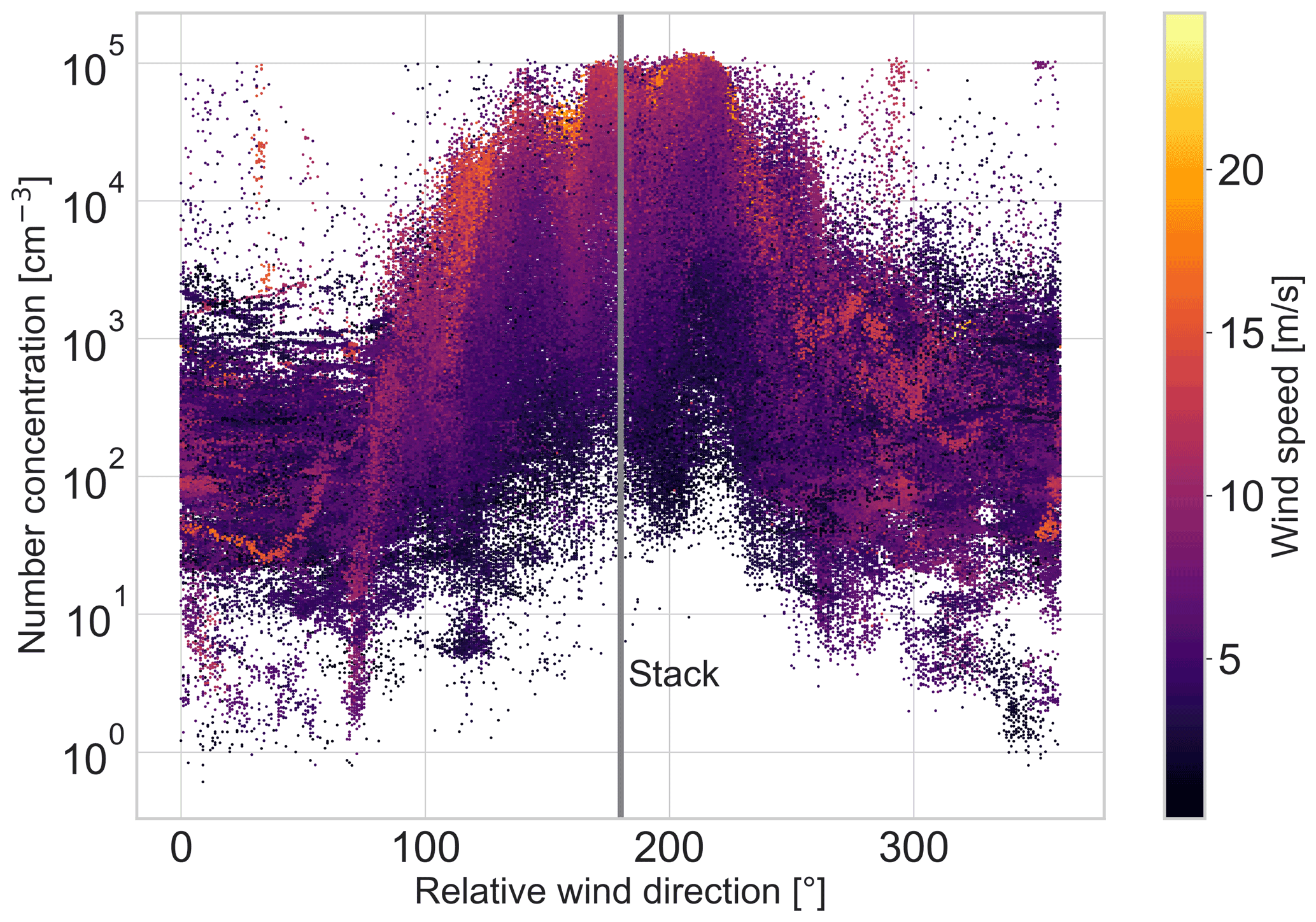
Figure 1 Particle number concentrations averaged over 1 min as a function of relative wind direction (0^∘ indicates wind coming from the bow) and color-coded by relative wind speed. Concentrations were higher with winds from the broader direction of the stack (located at 180^∘ from the inlet position, this position is marked with a vertical line).

Generally, concentration data from remote regions, characterized by the absence of dominant local (anthropogenic) sources, vary only slowly with time compared to when influenced by local contamination. This means that the concentration gradient (time derivative) is small. In contrast, concentration data show distinct variations, such as rapid fluctuations, when affected by contamination from nearby sources (e.g., Fig. A4). The PDA builds on this abrupt variation in concentration and detects polluted data based on the rate and magnitude of change in the concentration signal over a given time period. The basic principle of the PDA was developed and used for the 2018 Microbiology-Ocean-Cloud-Coupling in the High Arctic (MOCCHA) campaign on the Swedish ice breaker Oden by Baccarini (2021). Here, we further develop this algorithm and test it against different datasets. Importantly, the algorithm is only based on target concentration data and does not rely on ancillary datasets, such as particle size distribution or meteorological variables.

2.1.3 Particle number size distribution data

Furthermore, we applied the PDA to a particle size distribution dataset collected by a Scanning Mobility Particle Sizer (SMPS). The custom-built SMPS (Schmale et al., 2017) was located in the Swiss Container behind the switching valve and recorded the size distribution of particles between 17 and 600 nm with a time resolution of 3 min. We applied the PDA to the SMPS integrated particle number concentration. The results are presented in Sect. 3.1.2.

2.1.4 Aerosol chemical composition data

In addition, we tested the performance of the PDA against the aerosol chemical composition dataset obtained by the High-Resolution Time-of-Flight Aerosol Mass Spectrometer (HR-ToF-AMS) from Aerodyne Research Inc., located in the Swiss Container. The AMS measures the chemical composition of non-refractory aerosols, i.e., species that evaporate at temperatures up to 600 ^∘C. It typically detects sulfate (SO${}_{\mathrm{4}}^{\mathrm{2}-}$), nitrate (NO${}_{\mathrm{3}}^{-}$), ammonium (NH${}_{\mathrm{4}}^{+}$), chloride (Cl⁻), and organics (DeCarlo et al., 2006) from particles in the size range 0.07–1 µm, defined by the type of aerodynamic lens. The AMS was operated behind the switching valve to sample both interstitial and total inlet aerosol populations. Here, we use the mass signal of the ion fragment C₄H${}_{\mathrm{9}}^{+}$ at a mass-to-charge ratio of $m/z=\mathrm{57}$. This fragment is a typical indicator of fresh fossil fuel combustion (Enroth et al., 2016; Massoli et al., 2012) and has been used before to detect contamination in remote regions (Schmale et al., 2013). The results of the application of the PDA to the chemical composition data will be discussed in Sect. 3.3.1.

2.1.5 Trace gas data

We also used trace gas data collected in the Swiss Container to test the algorithm on datasets other than particle number concentration (Sect. 3.3.2). A detailed description of trace gas measurements during the MOSAiC expedition is given in Angot et al. (2022b). Briefly, carbon dioxide (CO₂), methane (CH₄), and CO ambient air mixing ratios were monitored by cavity ring-down spectroscopy using a Picarro instrument (model G2401) behind the interstitial inlet. Regular calibrations were carried out during the expedition with gas mixtures of known CO₂, CH₄, and CO mixing ratios.

2.1.6 Wind data

Wind speed and direction were measured with a 2D sonic anemometer on the main mast of RV Polarstern. We used this wind dataset at a time resolution of 1 min in this study (Schmithuesen, 2021a, b, c, d, e).

2.2 Wind-based filtering method

The main source of local pollution during the MOSAiC expedition was the stack of the ship. Based on Fig. 1, it is possible to define a polluted wind sector from 90 to 270^∘ relative to the bow of the ship. The wind-based filter flags all data points collected when the relative wind direction was coming from the polluted sector. This wind filter is introduced here for comparative purposes only. The comparison of the wind-based filtering method to the PDA is presented in Sect. 3.2.1.

2.3 Visual filtering method

The following visual filtering method is introduced here for comparative purposes: every pollution filtering method contains a certain level of subjectivity since the final decision about polluted versus non-polluted must be made by the user. Therefore, we compared the performance of the PDA to the result of a visual-only filtering method, which was applied to the dataset of the CPCf. Impact from local contamination is often evident from the time series of pollution-related variables, such as wind direction, wind speed, total particle number concentration, 1 standard deviation of particle number concentration within 1 min periods (N_{SD_1 m}), and particle number size distribution. Time series of these variables were visually inspected for each day to identify the periods impacted by the local contamination. N_{SD_1 m} was used as the core feature of pollution influence. In periods unaffected by pollution, it was below 30 cm⁻³. When the total particle number concentration was higher than ∼600 cm⁻³ (such as during new particle formation events in the summertime or during Arctic haze events in the wintertime), N_{SD_1 m} often increased to between 30 and 100 cm⁻³. However, these periods were not treated as local contamination influenced. Data were flagged as polluted when N_{SD_1 m} was above 10³ cm⁻³, the Aitken mode particle (i.e., diameter below 100 nm) number concentration was greatly enhanced, and wind was coming from the stack direction. Periods moderately influenced by the local contamination, during which N_{SD_1 m} was typically between 10² and 10³ cm⁻³ and the wind direction was usually not directly from the stack direction, are also flagged in this dataset. The visual filtering method also considered spikes and neighboring points. A spike of N_{SD_1 m} was defined as a point with a value that was 2 times higher than the 5 min moving average of N_{SD_1 m}. When two polluted flags were within 5 min of each other, all data points in between were flagged as polluted.

2.4 PDA

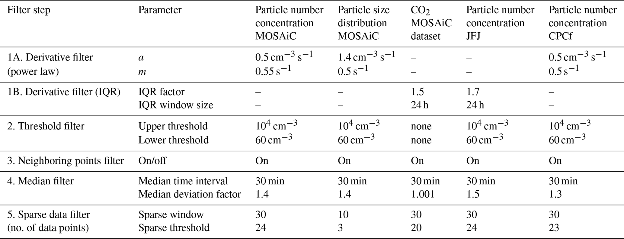
The PDA consists of a set of filters which can be applied in various combinations to identify polluted data. Figure 2 shows a schematic of the workflow. First, data points with a derivative exceeding a given threshold are tagged as polluted (Sect. 2.4.1). Second, a simple threshold filter tags data points which exceed a specific threshold, e.g., >10⁴ cm⁻³ in our case, because such concentrations are beyond the expected range for the central Arctic (see Sect. 2.4.1). Optionally, for every tagged data point, the neighboring point can be tagged too (Sect. 2.4.2). An optional median filter identifies outliers in the dataset which are left untagged (Sect. 2.4.3). Lastly, sparse data points left untagged in a series of tagged data points are also tagged (Sect. 2.4.4). Individual parameters and thresholds in each step can be adjusted to customize the PDA and to adjust its strictness. The neighboring and statistical median filters are optional and can be skipped, for example, if the resulting segregation of polluted data points satisfies the needs of the user already after the first steps. This allows retention of more data points in the final dataset. The different steps of the PDA are explained in detail in the following subsections. Table 1 summarizes all the parameters of the PDA described in Sect. 2.

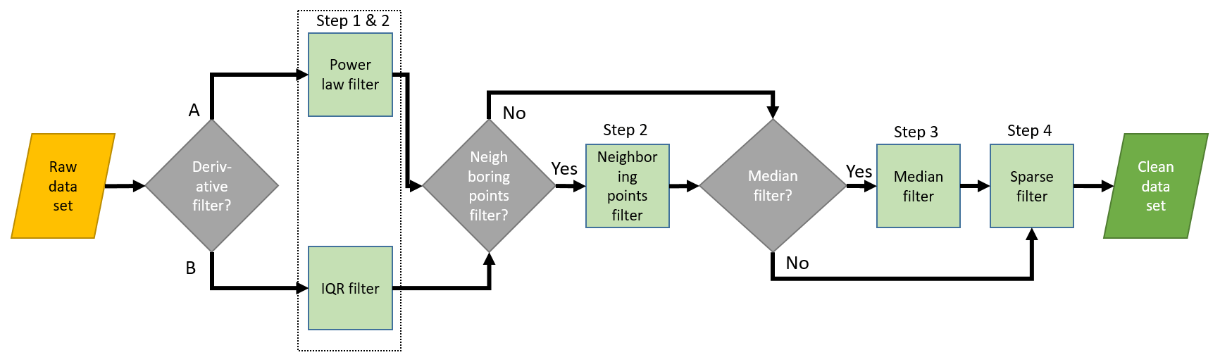
Figure 2 Schematic of the pollution detection algorithm. The key is the power law filter (highlighted in a dotted rectangle), which is followed by a series of steps. The neighboring points and the median filter are optional and can be skipped. Parameters of each step can be adjusted. IQR stands for interquartile range (see Sect. 2.4.1).

Table 1 Overview of all filter steps and parameters of the PDA applied to different datasets.

2.4.1 Steps 1 and 2: derivative and threshold filters

The derivative filter is used to separate periods characterized by rapid fluctuations in concentrations (we consider them to be polluted periods) from those dominated by slow changes in concentration (we consider them to be unaffected periods). At each data point at the native time resolution (10 s in our dataset) we calculate the absolute value of the time derivative (i.e., change in concentration) of the concentration using the central differences formula.

$$\begin{array}{}\text{(1)}& \left|\mathrm{d}C{{}^{\prime }}_t\right|\approx \left|{\displaystyle \frac{C_{t+\mathrm{1}}-C_{t-\mathrm{1}}}{\mathrm{2}}}\right|,\end{array}$$

where $\mathrm{d}C{{}^{\prime }}_t$ refers to the derivative of concentration C at time t, and C_t+1 and C_t−1 refer to the previous and following measured concentrations at times (t+1) and (t−1), respectively. Note that the derivative cannot be calculated with Eq. (1) at the edges of the dataset (very first and very last data points in the time series). Instead of the derivatives, the algorithm calculates the difference between the first (last) two data points at the beginning (end) of the dataset and uses those values for the derivative filter. This ensures that the edges of the dataset are also considered in the PDA. The derivative filter also ignores data gaps. For data points at the beginning and the end of a data gap, the derivative will still be calculated considering the previous and following data points, regardless of the duration of the gap (see Eq. 1). To separate polluted from unaffected data, we developed two methods.

Method A separates polluted from unaffected data with a power law. We average the time derivatives of the particle number concentration over 1 min (six values) and plot them against the 1 min-averaged particle number concentrations (Fig. 3). The averaging time can be varied and adapted to datasets with different time resolutions. This is discussed in Appendix C. We choose 1 min for a pragmatic reason: at 1 min time resolution we can still see influences of short-lived changes in particle number concentration (e.g., from contamination), and it makes data processing faster as the size of the 1-year-long dataset is large. Figure 3a shows two “branches” of data points (visually emphasized by the relative wind direction color code): one with higher derivatives representing periods of high concentration variability, i.e., due to local contamination, and one with lower derivatives, indicating smooth variation, i.e., not affected by local contamination. Separating the polluted and unaffected branches is the fundamental step of the PDA developed here. The derivative of the particle number concentration can be described as a power law of the particle number concentration, and the two branches distribute around two different power laws. Thus, for the separation, we use a power law between those two branches:

$$\begin{array}{}\text{(2)}& \left(y=a\times x^m\right).\end{array}$$

m corresponds to the slope and log (a) to the intercept with the logarithmic y axis. Values for the power law fits are empirically selected.

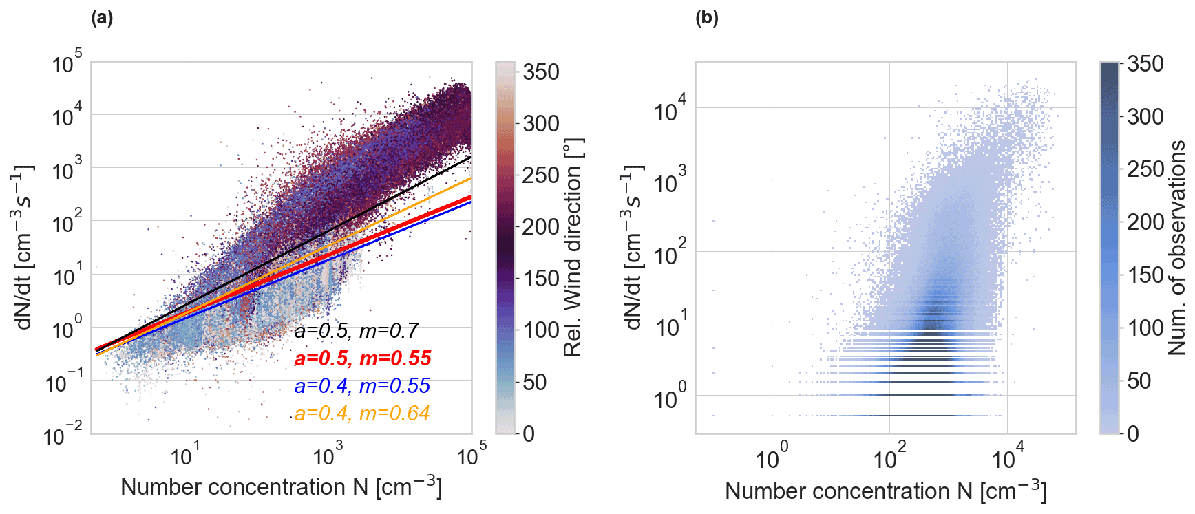
Figure 3 Absolute value of the minute-averaged particle number concentration derivative as a function of the minute-averaged particle number concentration. (a) The dataset collected during the MOSAiC expedition. The color code indicates the relative wind direction. The four lines show potential separation lines between polluted and unaffected data points for four different combinations of slope and intercept ($y=a\times x^m$). Here we used the red line. (b) The binned dataset collected at Jungfraujoch station in the Swiss Alps in 2016 (Bukowiecki et al., 2021). The color code indicates the number of observations per bin.

Finding optimal values for a and m is an empirical process which can be validated by looking at the time series of the polluted and unaffected data together. This process likely needs several iterations until values for a and m are found which satisfy the needs of the intended data analysis. A higher slope in the separation line means that, for a fixed particle number concentration, the threshold of separation moves towards higher derivatives of particle number concentration and therefore allows more variability in the data; i.e., the method is less strict. A higher intercept sets the threshold of separation to higher derivatives at lower concentrations, allowing for more variability there. Examples of four different separation lines are shown in Fig. 3a. For the MOSAiC dataset, we found values of m=0.55 s⁻¹ and a=0.5 cm⁻³ s⁻¹ (red line) to work well with our dataset (see Sect. 3.1).

Method B separates data based on the interquartile range (IQR) of the derivatives within a defined period. Not all datasets show an equally clear separation of the derivatives into two branches like the particle number concentration shown in Fig. 3a. An example is the particle number concentration dataset from Jungfraujoch (Fig. 3b). An alternative method is thus to separate polluted from unaffected data based on the deviation of the derivatives from their centered IQR. For this, we calculate the centered IQR of the derivatives of each data point in a moving time window (called the IQR window) (24 h in the case study described in Sect. 3.3.3, which is equal to 1440 data points). This means that, for each data point, we calculate the IQR from the data ± half of the IQR window before and after the data point. When the absolute derivative of a data point exceeds the 75th percentile by a given factor (hereafter called the IQR factor), the data point is flagged. We use an IQR factor of 1.7 to identify contamination in the JFJ dataset. Both the IQR window size and the IQR factor of the IQR method can be adjusted in the PDA code. Method B is well suited to separating datasets with less obvious differences between polluted and unaffected periods. As a first start, we therefore suggest trying an IQR window size of 1440× x, where x is the time resolution of the dataset. We found the factor 1440 to work for datasets with 1 min time resolution, where it represents a time window of 24 h.

Note that the moving centered IQR can only be calculated for data points with a distance of half of the IQR window from the edges in the dataset. To also account for the edges of the dataset, we fill the first (last) data points with the calculated IQR value of the first (last) calculated data point. This means that the IQR is assumed constant for half of the IQR time window at the edges. In our case (with an IQR window of 24 h), this affects the first and last 12 h of the dataset.

Simultaneously with the derivative filter, we introduce upper and lower concentration thresholds (step 2), as described below, beyond which data are removed. For specific regions, like the central Arctic in our case, one can assume concentrations not to exceed a certain threshold as long as they are not influenced by local contamination sources. Based on the particle number concentration dataset throughout the whole MOSAiC and MOCCHA observation periods, we argue that it is safe to assume that particle number concentrations above 10⁴ cm⁻³ can be considered to be influenced by local contamination with the detection limits of the instruments used for the two campaigns. Note that new particle formation events, which typically lead to the highest number concentrations second to ship activities during the expedition, do not exceed this threshold. See Fig. 3, where the branch of unaffected data below the separation line does not show any data points >10⁴ cm⁻³. A similar principle is applied to a lower limit, here 60 cm⁻³. Below this threshold, we assume the dataset is not influenced by contamination. This threshold helps to maintain the background when a sudden concentration drop (e.g., from a precipitation event) would trigger the derivative filter. We choose 60 cm⁻³ to be a suitable threshold for this dataset because we did not observe such low values during polluted time periods, except on very rare occasions, but those data points would be detected by the sparse filter (Sect. 2.4.4). Both thresholds can be adjusted in the tool, because they will vary with location, the detection limit of the instrument, averaging time, and target compound. For example, a higher lower-limit threshold might be appropriate in a remote forest region, where lower particle number concentration limits can be as high as 500 cm⁻³ (Schmale et al., 2018). If the lower threshold is set to zero, all data below the upper-limit threshold are included in the filtering algorithm. The threshold filter activates automatically with the application of the derivative filter. Hereafter we also mean the threshold filter when we talk about the derivative filter.

2.4.2 Step 3: neighboring points filter

It can be useful to discard points at the beginning and end of polluted periods where single data points might not be tagged because the deviation of their values from previous or subsequent points is too small to be detected by the PDA. This filter targets data points at the transition from polluted to unaffected periods and vice versa. Applying this filter is optional as it discards additional data but in return results in a dataset less affected by local contamination. We show and discuss the results of this step in Sect. 3.1.

2.4.3 Step 4: median filter

The median filter aims at detecting false negatives, i.e., data points which are not representative of the background signal but which were not flagged by the previous filter. For each data point, we calculate its deviation from the running median over a time interval (the median time interval). If the deviation exceeds a given factor above this median, it is flagged as polluted. The factor can be adjusted to lower (stricter) or higher (less strict) values with the trade-off of more false positive data points (i.e., unaffected data points flagged as polluted) or false negative data points (i.e., polluted data points which are not flagged), respectively. We found an empirical deviation factor of 1.4 to support the detection of outliers for MOSAiC and keep the number of false positively detected data points as small as possible. This is further discussed in Sect. 3.1.

2.4.4 Step 5: sparse data filter

As a last step, we apply a sparse data filter to tag leftover unaffected data points in periods affected by local contamination. More quantitatively, if the number of polluted data points in a given time window (subsequently called a sparse window) exceeds a given threshold (termed a sparse threshold), all points in the sparse window are flagged as polluted. We use a sparse threshold of 24 within 30 data points (which corresponds to 30 min in our case). The sparse threshold and the associated time window can be adjusted in the PDA. The sparse data filter is automatically activated as the final filtering step. To de-activate the sparse data filter, one can simply set the sparse threshold to the same number of data points as in the sparse window.

3 Results and discussion

In this section, we present and discuss the performance of the PDA and compare the results to other commonly used approaches to identify local contamination (wind direction and visual inspection methods). We test the PDA on different types of atmospheric measurements as well as on particle number concentration datasets with different time resolutions.

3.1 Performance of the PDA

First, we demonstrate the effect of the successive application of the various pollution filter steps, and second, we evaluate the performance of the final PDA settings against characteristic situations from the MOSAiC expedition. While the algorithm was applied to the entire dataset, below we show 24 h case studies to illustrate the results.

Figure 4a–c show, for the case study from 6 March 2020, how the individual filtering steps (the derivative filter, the derivative filter combined with the neighboring points filter, and all filters together) affect the final cleaned particle number concentration dataset. The original time series is marked in red, while the cleaned dataset appears in blue. The case study shows a stable signal with concentrations around 100 cm⁻³, which is interrupted by a pollution event with particle number concentrations up to 10⁵ cm⁻³ from 09:00 to 12:00 UTC. The derivative filter (Fig. 4a) detects the majority of the polluted data points. Only 10 data points in this period remain untagged. Including the neighboring points filter (Fig. 4b) and the median and sparse data filters (Fig. 4c) removes all those points, improving the performance of the algorithm. Figure 4d shows histograms of the entire MOSAiC particle number concentration record for the original dataset and, after application of the derivative filter, the derivative and neighboring points filter and all filters. Concentrations below 200 cm⁻³ remain nearly untouched by all filters in the PDA. The strongest filter effect is visible at larger number concentrations (>3000 cm⁻³), where only a few counts remain in the cleaned dataset. In accordance with the threshold filter, number concentrations above 10⁴ cm⁻³ are removed. The application of all the filters combined is not always necessary, as shown in Fig. A6. Here, the derivative filter already detects all the polluted data points, and no further filters are needed. Table 2 shows how the year-round dataset is reduced in size after applying the derivative filter, the derivative and neighboring points filters, or all filters combined. The second row shows the percentage of the original dataset that is left after applying the respective filters. After application of the derivative (and threshold) filter, 44 % of the data points are retained, showing the importance of the application of a filtering method in general. Applying further filtering with the neighboring points and median filters removes only 5 % and 1 % of additional data points, respectively. This demonstrates that the derivative filter alone captures the majority of locally polluted data points (90 %), while the additional filters have a “fine-tuning” effect. This effect can still be very important for individual cases as shown in Fig. 4a–c. Figure A7 summarizes the percentage of clean data per day after application of the PDA for the whole expedition. The data were most affected from contamination in spring and summer and least affected in winter. Note that this graph is indicative of contamination visible in the particle number concentration data and not necessarily for all atmospheric chemical and microphysical measurements taken during MOSAiC. To assess the effect of each filtering step, we applied each of them individually to the CPC3025 dataset and discuss this in Appendix B.

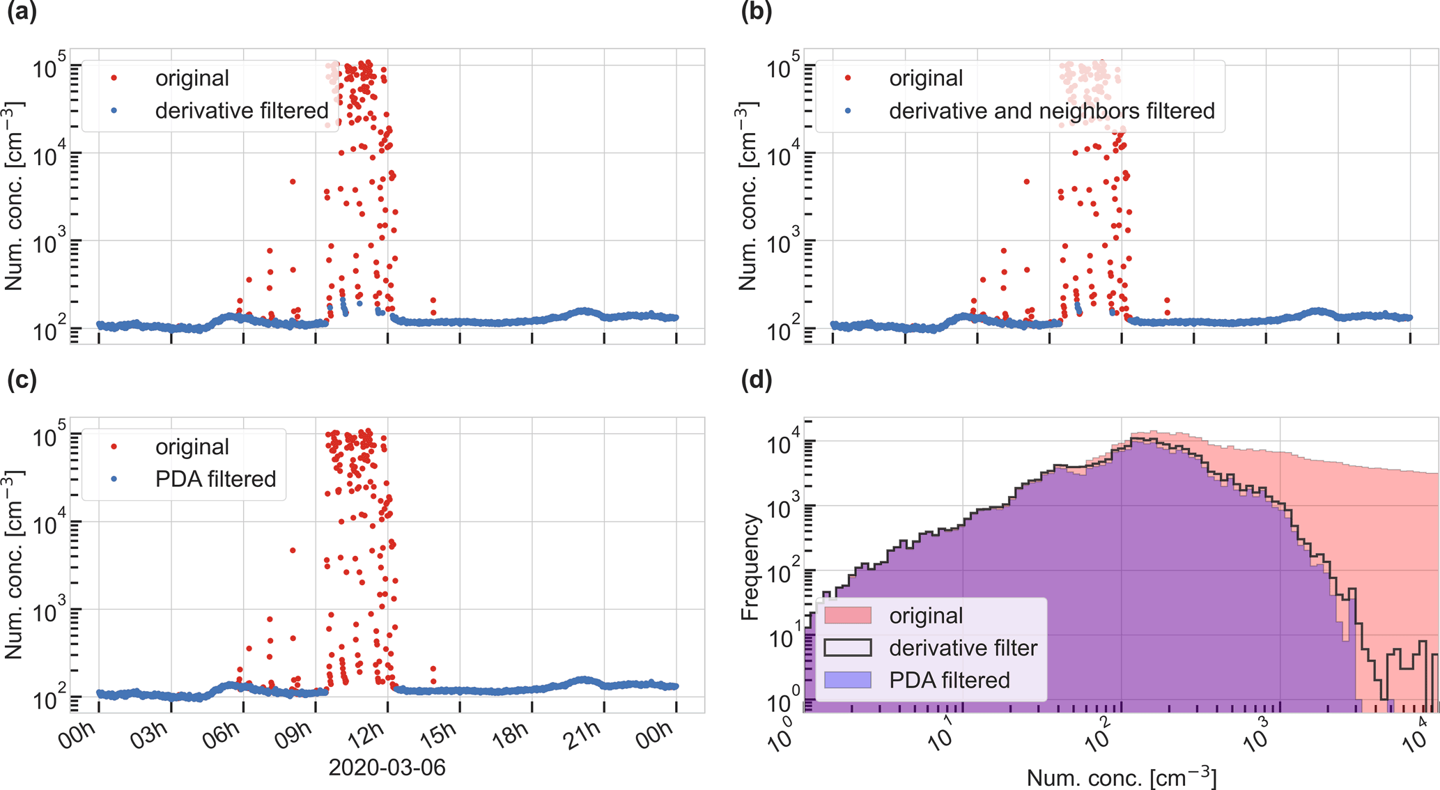
Figure 4 Comparison of the derivative filtering method with additional filtering steps. Cleaned data (in blue) are plotted over raw data (in red). (a) Only derivative filter applied. (b) Derivative and neighboring points filters applied. (c) All filters applied. (d) Histogram of the original (in red) and remaining datasets after steps (a) (black contour line) and (c) (purple). “PDA filtered” means all options of the PDA were applied. For all plots we used data from the CPC3025. Raw data have only been pre-cleaned for zero filter measurements. The orange circles indicate areas where the additional filters remove additional data points.

Table 2 Number of data points and percentage (relative to raw data) of data left when different filtering steps are applied.

3.1.1 Case studies

Particle number concentrations in the Arctic can vary by orders of magnitude. To verify that the algorithm can be used under different environmental and contamination conditions, we tested its performance in characteristic situations throughout the expedition.

First, under conditions when the dataset is not affected by strong pollution spikes, it is required that the algorithm still detects small influences from local contamination. Figure 5a shows a day in January with a very stable and low boundary layer, resulting in a stable particle number concentration background around 150 cm⁻³ and occasional pollution spikes around 12:00. The algorithm successfully detects polluted data points and leaves the background untouched. In contrast, the wind filter would not detect any of the contamination. In this case, a stricter wind filter would not be possible since it would basically have to be extended to all wind directions. Second, under very polluted conditions, the requirement for the algorithm is to detect the full contaminated period and to not leave polluted data points undetected (false negatives).

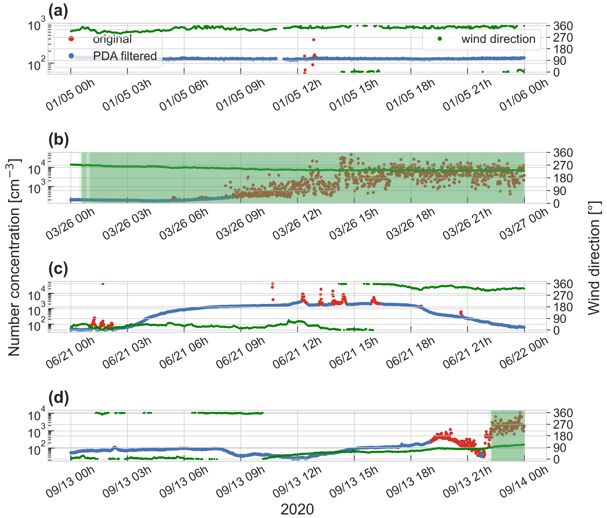
Figure 5 Performance test of the PDA method in four different situations. (a) Under overall stable conditions, (b) transition from clean to polluted conditions, (c) a natural increase in particle number concentration due to new particle formation, and (d) a natural decrease in particle number concentration due to a precipitation event (freezing rain) in the morning (from 09:00 to 12:00 UTC). Green shaded areas indicate where the wind filter would flag data as polluted. Green points show the wind direction, and red points show the raw particle number concentration, overlaid with the cleaned data points in blue.

In Fig. 5b, a transition from unaffected to polluted conditions can be seen around 09:00 UTC due to changes in wind direction that resulted in stack exhaust contamination. The variability in the signal increases strongly, and so does the gradient between data points. The PDA detects all relevant points as pollution. The wind filter would, in this case, also detect all the relevant points but would become effective much earlier and thus detect false positives.

Third, new particle formation (NPF) and subsequent growth of particles are common processes in the Arctic which lead to an increase in particle number concentrations over a relatively short time (Kulmala et al., 2014; Baccarini et al., 2020; Schmale and Baccarini, 2021; L. J. Beck et al., 2021). This could potentially cause the derivative algorithm to accidentally flag naturally high concentrations as pollution (false positives). We analyze one NPF event observed on 21 June 2020 where the particle number concentration increased from <100 cm⁻³ to more than 1000 cm⁻³ within 3 h (Fig. 5c). In addition, a few pollution spikes were observed during the NPF event. The derivative filter detects the pollution spikes and leaves the background untouched during the NPF-driven rise as well as during the subsequent drop in particle number concentration later in the day. If a specific case study on this NPF event was done, the user could decide to apply the PDA only to this event and to tune the parameters specifically. Here we show that the settings chosen for the entire campaign treat the NPF event adequately.

Fourth, another potentially challenging situation for the algorithm is wet-removal events. Aerosols can be washed out of the atmosphere by rain or snow and their number concentration can decrease quickly, leading to elevated derivatives. We report such an event observed on 13 September 2020 from 09:00 to 12:00 UTC (Fig. 5d). The rate of change of the particle number concentration is not strong enough to cause false positives. These results demonstrate that the algorithm is able to deal with relevant situations and is therefore an adequate tool to clean particle number concentration datasets, which are influenced by both natural variability and local contamination sources.

To verify that the spikes in particle number concentration are caused by pollution and not by a natural local (or regional) event, we compare the particle number concentration data during a pollution event on 27 July to several other signals like nitric oxide (NO), CO, and BC (Fig. A4). The main pollution spike in this example (ca. 18:00 UTC) coincides with the NO signal, which also shows a distinct spike at the same time (panel a). The BC signal also reacts during this event with elevated concentrations (panel d). The CO signal does not react at this time. Note that the CO signal does not react strongly to ship pollution. This is in agreement with what we observed during the expedition and highlights the issues in operating the automated purge system in the AOS container (Sect. 2.1.1). The ship exhaust from RV Polarstern during the MOSAiC expedition did not consistently show elevated CO signals that could allow CO to be used to identify pollution reliably. However, there were cases where apparent pollution events did result in higher observed CO concentrations. During the event described here, there are two minor spikes at 08:00 and 10:00 UTC where the particle number concentration shows spikes that coincide with the CO signal (panel b). In contrast to the first example at 18:00 UTC, the wind direction was not coming from the stack. This points towards a different local source of contamination, e.g., a skidoo, snow groomer, or ship vent. These indicators lead us to conclude that the particle number concentration signal is sensitive to contamination from different sources and therefore provides a good basis for the development of the PDA.

3.1.2 Application of the PDA to particle size distribution

We applied the PDA with the parameters given in Table 1 to the measured total particle number concentration time series (i.e., the sum of the concentrations of all size bins) of an SMPS dataset, collected during the MOSAiC expedition in the Swiss Container. The result is shown in Fig. 6 on a 7 d subset of the particle size distribution (PSD) dataset. The polluted periods are clearly visible in the PSD and show as distinct yellow vertical lines. At the same time, the total number concentration shows strong spikes. The PDA detects the polluted periods (shown as red data points) and leaves unaffected data (shown as black data points). This validates the functionality of the PDA. The SMPS data have a time resolution of 3 min, which shows the ability of the PDA to detect contamination in datasets with different time resolutions. More tests of the PDA with datasets of different time resolutions are discussed in Appendix C.

Figure 6 Application of the PDA to the total number concentration dataset (black line) collected by an SMPS. Data points identified as polluted by the PDA are marked in red. The dataset is plotted over the particle size distribution data of the same instrument.

3.2 Comparison of the PDA to other commonly used methods

3.2.1 Comparison to the wind filter

The majority of pollution events are associated with wind arriving from the direction of the stack of the ship (Fig. 1). Thus, applying a simple filter based on wind direction might be sufficient to discard most polluted data. An example is shown in Fig. 7, where we assumed a polluted wind sector between 90 and 270^∘ and marked all tagged data points with a red band. The wind filter flags 59 % of the data as polluted compared to the PDA, which flags 62 %. However, apart from detecting a large portion of polluted data, it also creates false positives; i.e., it flags unaffected data as polluted, as described in Sect. 3.1. It also does not detect any polluted data outside of the polluted wind sector. This is illustrated in Fig. 8 for 17 February 2020, where we compare the wind filter (panel b) with the PDA (panel a). On that day, the wind came from the port side of the ship and carried polluted air from a snow groomer. The PDA (panel a) detects and tags more polluted data than the wind filter (panel b). In addition, the PDA allows unaffected data in the polluted wind sector to be kept (Fig. 7). The wind direction method might, however, be simple and easy to clean data when the only source of local pollution is a point source and if the only contamination source is in a fixed wind direction from the measurement point. Although widely used in ship campaigns (see Sect. 1), the wind filter is not well suited for those campaigns where multiple and moving emission sources exist.

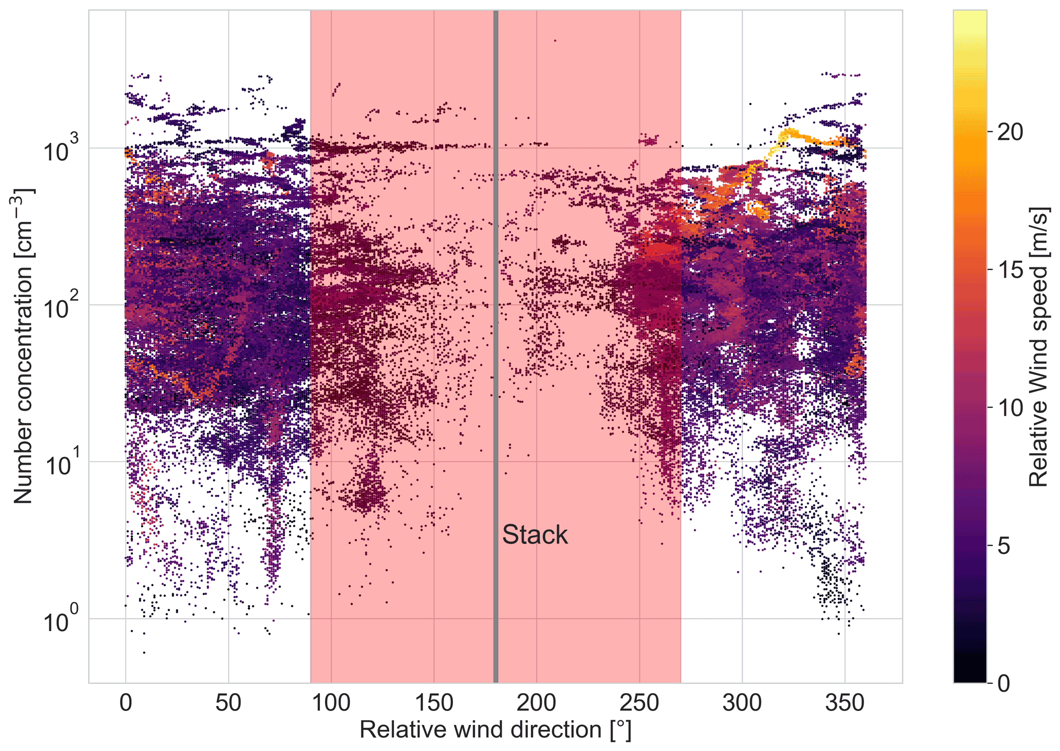
Figure 7 Same as Fig. 1 but after applying the PDA to the dataset. Flagged data points were removed to visualize the data product after application of all filtering steps. The red shaded area indicates where the wind filter would flag polluted data (between 90 and 270^∘ relative to the bow). The direction of the stack is marked at 180^∘ as a vertical line.

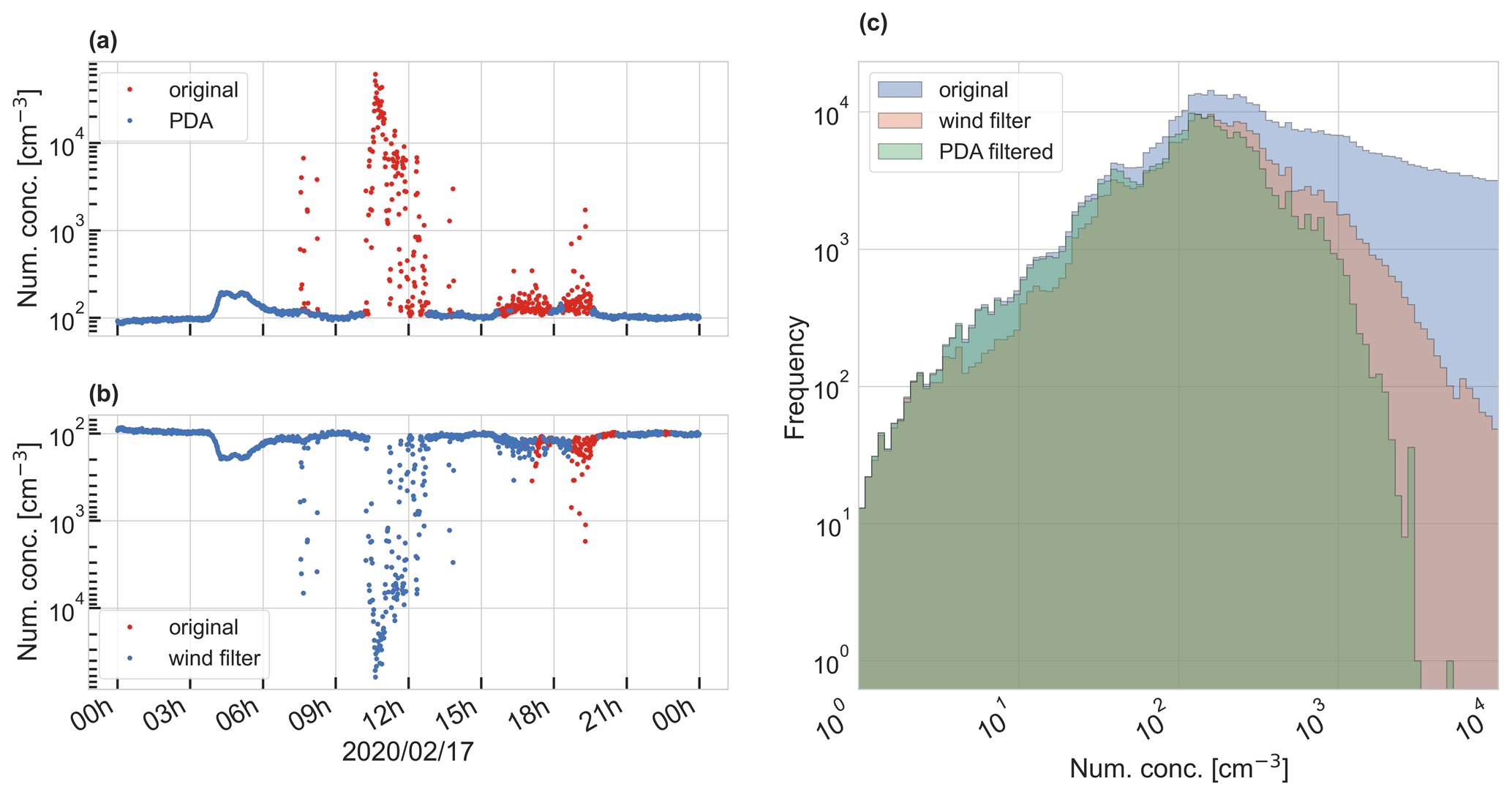
Figure 8 Comparison of the PDA (a) with the wind-based method, assuming a polluted-air sector of 90 to 270^∘ from the bow (b, mirrored). Both filtered time series (blue) are underlain with the original raw data (red). The wind-based filter method cannot detect pollution events coming from other directions than the given wind sector. Panel (c) shows histograms of particle number concentrations before (blue) and after application of the PDA (green) and the wind mask (red).

3.2.2 Comparison of the PDA to the visual inspection method

We applied the PDA to a dataset independently cleaned by visual inspection and compared the results of these two methods. The dataset used for this test was collected from the ARM AOS container during the MOSAiC expedition. The visual filtering method is described in Sect. 2.3. The parameters used to apply the PDA to the dataset are listed in Table 1.

Both methods detect roughly the same fraction of clean data and agree in 93.9 % of all data points (see Table 3). The visual filtering method identifies slightly more clean data. Figure 9 shows the results of both methods in histograms. It shows the distribution of the raw data points (in gray) and the fraction of data points where the two methods do not agree, i.e., the fraction of data points which are identified as clean by the visual inspection but not by the PDA and vice versa.

Table 3 Fraction of clean data points of the derivative filtering method and the visual filtering method compared to the total number of data points (total counts) in numbers and in percent of the total counts. This table is based on the CPCf dataset at 1 min time resolution.

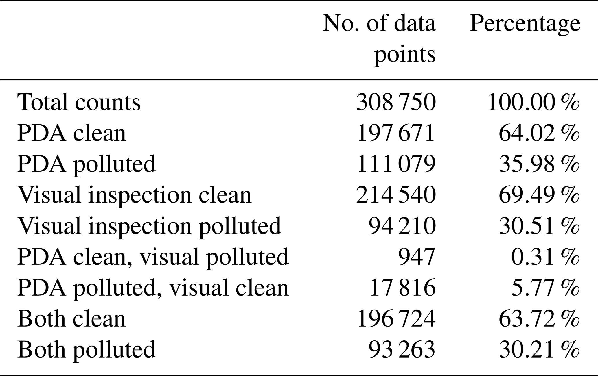
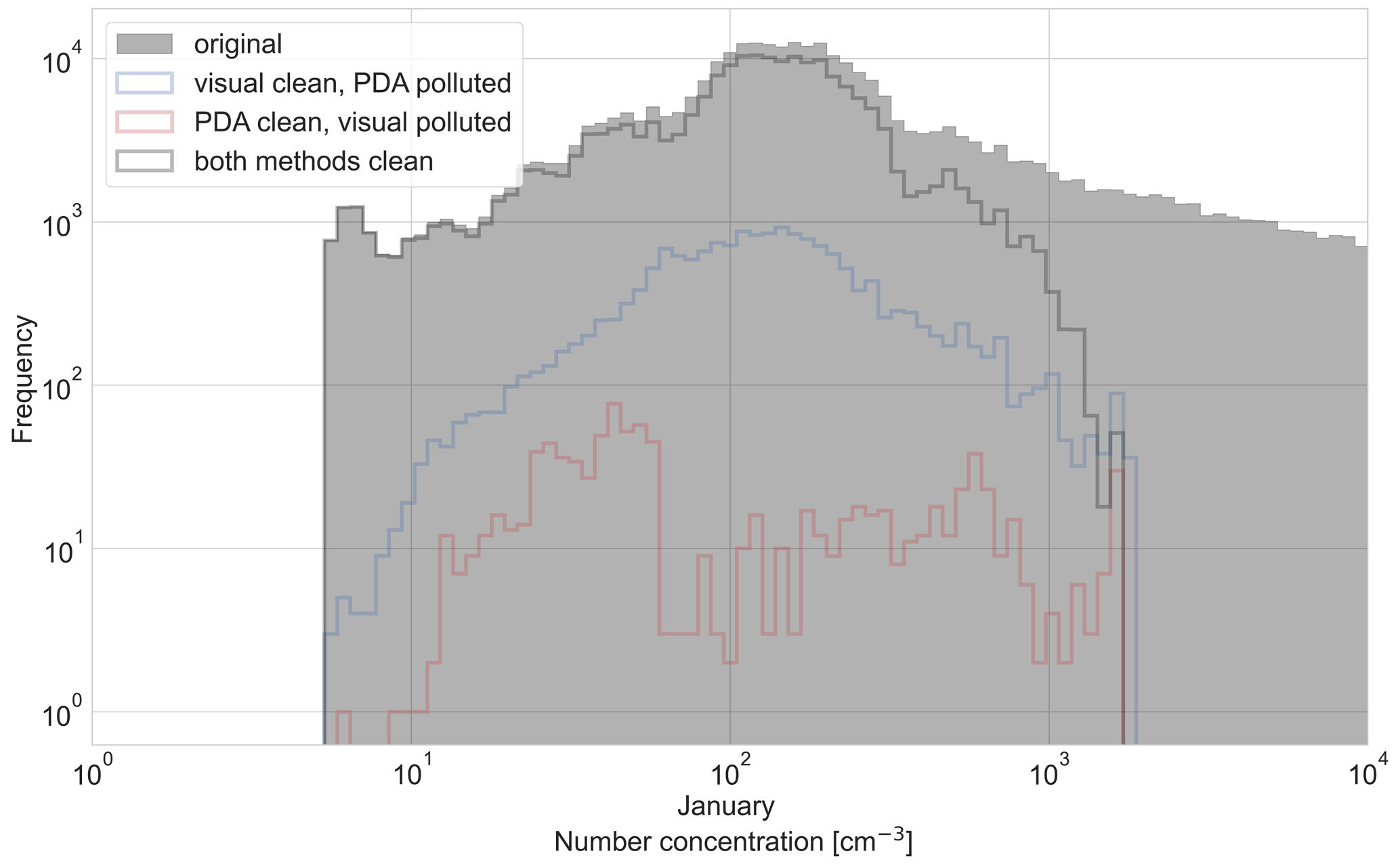
Figure 9 Comparison of the visual inspection method to the PDA on the dataset of the CPCf of ARM. Original data are shown in gray. The blue contour line shows the fraction of data points where only the visual inspection method but not the PDA considered data to be clean (6 %). The red contour line shows the opposite, i.e., the fraction of data points where only the PDA but not the visual inspection method considered data to be clean (<1 %). The dark gray contour line shows the fraction of data points where both methods considered data to be clean (∼64 %).

The fact that the visual method keeps slightly more data points unaffected at lower concentrations compared to the PDA could be an indication that visual inspection detects slightly fewer false positives (unaffected data points detected as polluted). However, the advantage of the PDA is that it can be applied to other datasets with relatively little effort. Also, it applies strict thresholds to the dataset, which makes the result reproducible, while the visual filtering method depends on the users and their experience, which makes it more prone to user bias. A comparison of both filtering methods in a time series is shown in Fig. A8.

3.3 Broader application of the PDA

We test the performance of the PDA on datasets with different characteristics using time series of particle chemical composition and ambient air CO₂ concentrations collected during MOSAiC (Sect. 3.3.1 and 3.3.2, respectively) and on a particle number concentration dataset collected at JFJ in the Swiss Alps (Sect. 3.3.3).

3.3.1 Application to aerosol chemical composition datasets

To check whether the algorithm works on other datasets than particle number concentration data, we applied it to the ion fragment signal of C₄H${}_{\mathrm{9}}^{+}$ ($m/z=\mathrm{57}$) measured by the AMS, which characterizes fresh contamination from combustion. In a perfect scenario, our developed algorithm is able to group the signal of this fragment (C₄H${}_{\mathrm{9}}^{+}$) into high mass (and high derivative) resulting from ship emissions in comparison to low background mass concentration (and low derivative), the latter associated with a relative wind direction away from the stack (90 to 270^∘ relative to the bow). Figure 10a shows the relation of the derivative of the mass concentration of C₄H${}_{\mathrm{9}}^{+}$ (averaged over 5 min) as a function of its mass concentration. We observe a separation of the derivatives into two branches with two different slopes as in Fig. 3a. However, the mass concentrations do not overlap in the two branches of the derivatives $(\mathrm{d}M/\mathrm{d}t)$ of clean and polluted periods, and therefore a separation based on the derivative is impossible. This is also visible based on the wind direction (indicated by the color); a separation between the “pollution” and “clean” data points occurs at approximately 10⁻² µg m⁻³, resulting in a critical concentration threshold rather than a defined slope. However, such a separation at a defined mass concentration grouped certain “clean” data points into the “polluted” category and thereby failed to produce a reliable pollution mask. Our hypothesis for the failure of the derivative algorithm when applied to AMS data is that the AMS has a lower particle cut-off of 70 nm and the >70 nm particles detected by the AMS are affected by contamination in a different way than the entire particle population also containing smaller particles, as reflected by the CPC data, which contain particles as small as 3 nm. We found that the typical peak diameter of ship pollution observed on RV Polarstern was approximately 30 nm. An alternative way to produce a pollution tag for AMS data is to apply a chemically resolved method, where the mass spectrum as a whole is compared to a previously defined chemical pollution spectrum. This method is described in more detail in Dada et al. (2022).

Figure 10 (a) Derivative of the ion mass signal of C₄H${}_{\mathrm{9}}^{+}$ ($m/z=\mathrm{57}$) compared to its total mass concentration, measured by the AMS. (b) Derivative of the CO₂ concentration signal compared to its concentration, measured by cavity ring-down spectroscopy. Colors indicate the relative wind direction.

3.3.2 Application to trace gas datasets

Figure 10b shows the distribution of the derivatives for the CO₂ dataset. We used CO₂ data at a 1 s time resolution and averaged the derivative over 1 min. The CO₂ signal varies by less than 1 order of magnitude when affected by pollution. The majority of the data points do not deviate from the observed atmospheric background concentration of around 400 parts per million (ppm). The color-coded wind direction also gives no indication of separation of the data by wind direction. One reason is that the magnitude of the derivative of the CO₂ signal in case of pollution is low compared to its relatively high background concentration, and therefore polluted data points do not separate clearly from the main “branch” of data points. Therefore, the separation of polluted and unaffected data points based on two branches of derivatives (step 1A) does not work for the CO₂ dataset. We thus applied the PDA with step 1B (the derivative filter based on the deviation from the running interquartile range) to the CO₂ dataset. The parameters used for the PDA are shown in Table 1. An example of the resulting time series is shown in Fig. A9 on the same case study on 27 July as we described in Sect. 3.1.1. The CO₂ signal is noisy and shows a strong spike between 16:00 and 20:00 UTC. This spike matches the observations described in Fig. A4. The PDA detects and flags data points within the spike as polluted. Situations like this example with a noisy signal are further discussed in Sect. 3.4. Angot et al. (2022b) applied this method and describe the CO₂ dataset in more detail.

3.3.3 Application of the PDA to a long-term high-altitude site-monitoring dataset

We applied the PDA to a particle number concentration dataset collected at the high-altitude research station JFJ in the Swiss Alps. The data have a time resolution of 1 min. The calculated derivatives show a very different pattern compared to those from the MOSAiC expedition (Fig. 3a–b). The difference in magnitude between contamination and the JFJ background dataset is much smaller (Fig. A10) compared to MOSAiC. The JFJ dataset is therefore well suited for separating polluted data using the IQR filtering method (step 1B). The parameters used in the PDA are shown in Table 1. The PDA was applied to an example time series from 2 d in July 2016 (Fig. A10), where a diurnal cycle of the background and pollution spikes during daytime are visible. This example demonstrates how the background is distinguished from the spikes even when the background varies by an order of magnitude. Given the different approach by Bukowiecki et al. (2021), i.e., detecting and counting spikes versus masking polluted time periods with the PDA, we cannot make a direct comparison between the two methods like in Sect. 3.2.2 (visual method). The final decision about flagging individual data points remains the user's responsibility and will depend on the objective of the analysis.

3.4 Limitations of the PDA

This study shows that the PDA is capable of cleaning contamination from a variety of particle and trace gas datasets. However, a challenge for the algorithm remains to deal with false negatives, which are left after applying the derivative filter (step 1 of the PDA). In situations with small pollution peaks, which occur on top of a clean background, this is often the case at the beginning and at the end of the affected period. The application of the neighboring points filter on top of the derivative filter improves the result significantly but might not catch all pollution-affected points. An example of this is shown in Fig. A11a and b.

Another challenge for the PDA is situations where the signal is influenced by subtle contamination, which does not result in large spikes but rather in a very noisy signal with low amplitude above a background. Two examples are shown in Figs. A9 and A11. These situations are also difficult to assess for an expert using the visual inspection method. The boundary between polluted and unaffected data is blurred, and the derivative filter in Fig. A11 only flags a subset of data points that protrude from the main signal. In this example, some of the flagged data points do not exceed the “baseline” concentration at all. The difference between an unaffected and a flagged data point can be 2 cm⁻³ at concentrations of 190 cm⁻³ or 10 cm⁻³ at 390 cm⁻³ (the derivative filter threshold depends on the concentration). If we choose a stricter derivative filter, for example, with a=0.45 (instead of 0.5) and m=0.5 (instead of 0.55), more data points are flagged as contaminated and hence fewer false negatives remain (Fig. A12). However, this might also remove unaffected data points, and it is up to the user to make this decision.

The applicability of the PDA to a dataset also depends on the response time of the instrument. A response time which is slower than the occurrence of pollution (i.e., the instrument cannot capture the sharp rise and fall in concentrations) leads to smaller derivatives of the measured particle number concentrations. This would set an upper limit to the measured derivative. Still, pollution could be detected as long as this upper limit is substantially higher than the derivatives of the natural signal. This does not matter for the measurements with the CPCs, since the response time is typically lower than 1 s (Enroth et al., 2018). In essence, this issue is similar to recording data at a coarse time resolution, which would smear out the difference in magnitude between background and pollution (see Appendix C).

4 Conclusions

We developed a pollution detection algorithm (PDA) to identify periods of local contamination in atmospheric aerosol and trace gas concentration time series. The PDA was successfully tested with particle number concentration datasets from two different sites – a ship-based expedition in the high Arctic Ocean and a background station in the Swiss Alps affected by tourism – as well as with a CO₂ concentration dataset from the high Arctic. In comparison to the commonly used wind direction method to clean datasets, the PDA is capable of identifying contamination from different sources and directions and reduces false positive and false negative results. Compared to a visual filtering method, the PDA identifies a similar amount of contamination (41 % with the visual method compared to 43 % with the PDA). The PDA only uses the target concentration data and does not rely on ancillary datasets to identify polluted data points. It works for datasets with a relatively low background where pollution spikes exceed the background significantly and the sampling rate is fast enough so that the derivative of polluted signals separates clearly from that of unaffected ones. “Fast enough” depends on the variability of the background and occurrence of pollution. In our case the methods worked for time resolutions between 10 s and 10 min. The PDA is primarily designed for remote locations, but it might also be applied to locations where local contamination interference is so frequent that the majority of data points exceed the contribution from the underlying background in the period of interest, like in urban areas, for example.

The relative magnitude of interference from local contamination varies between different measurement campaigns and may depend on the type of instrument. The PDA is best suited to identifying primary pollution, i.e., for particle number concentration, trace gases directly emitted by the pollution source (e.g., CO₂), or size distribution datasets with a clear primary pollution mode. For other variables, such as for accumulation-mode particle chemical composition data, which are not representative of the main pollution size range (around 30 nm), a different approach might be better (e.g., Dada et al., 2022) because the PDA will discard too many data points.

The PDA is published open source in a user-friendly code toolkit downloadable from Beck et al. (2021) (see reference list). All PDA parameters can be adjusted to adapt it to specific datasets or to customize the filtering level for specific needs. This makes it flexible and allows its application to locations where no ancillary datasets might be available. It also allows a fast application to multiple datasets and provides an objective, reproducible method to identify local contamination under remote or background conditions.

Appendix A: Supporting figures

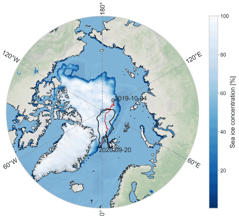
Figure A1 Track of RV Polarstern during the MOSAiC expedition in the central Arctic (Schmithuesen, 2021a, c, d, e, b). Drift (red line) started in October 2019 and ended in September 2020. The black lines show periods where the ship was in transit. The sea ice extent is displayed from September 2019 at the annual minimum. We used sea ice data from the National Snow and Ice Data Center (Maslanik and Stroeve, 1999). The background map is made with Natural Earth (https://www.naturalearthdata.com/, last access: 6 October 2021).

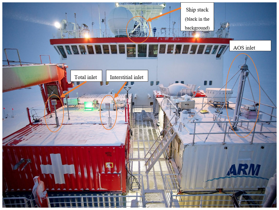
Figure A2 Bow of the ship during the expedition. In red with a white cross, the Swiss Container with its two inlets. The ARM measurements were performed on the port side of the ship in the white container at the front with a higher inlet. Photo credit: Michael Gutsche.

Figure A3 Full setup of the Swiss Container during the MOSAiC expedition (not all elements are discussed in this paper). In yellow the total inlet, in green the interstitial inlet. The valve switched between the two inlets to allow the instruments behind it (Aethalometer, AMS, SMPS, cloud condensation nuclei counter) to measure from both inlets. The blue inlet is the new particle formation inlet. CI-Api-ToF stands for chemical ionization atmospheric pressure interface time-of-flight mass spectrometer. NAIS stands for neutral cluster and air ion spectrometer.

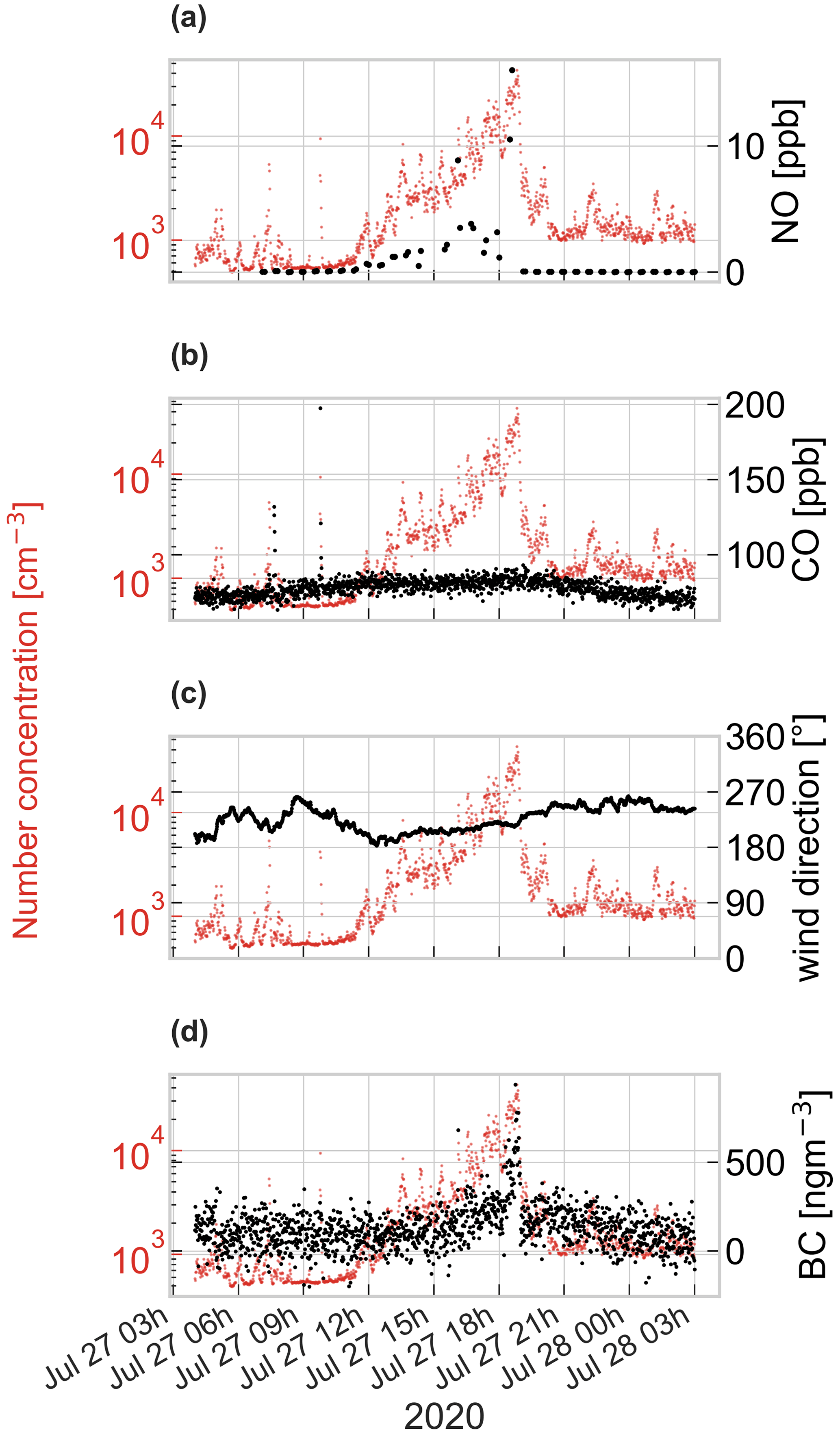
Figure A4 Particle number concentration (left axis) along with (a) NO (in parts per billion; ppb), (b) CO (ppb), (c) relative wind direction, and (d) equivalent BC (ng m⁻³) at 880 nm with standard manufacturer settings for the correction factor and mass absorption cross section during a local contamination event in the afternoon of 27 July 2020. Starting around 12:00, the particle number concentration and NO and BC concentrations increased as wind came from the stack. Note that CO concentrations did not exhibit any significant variability during that event.

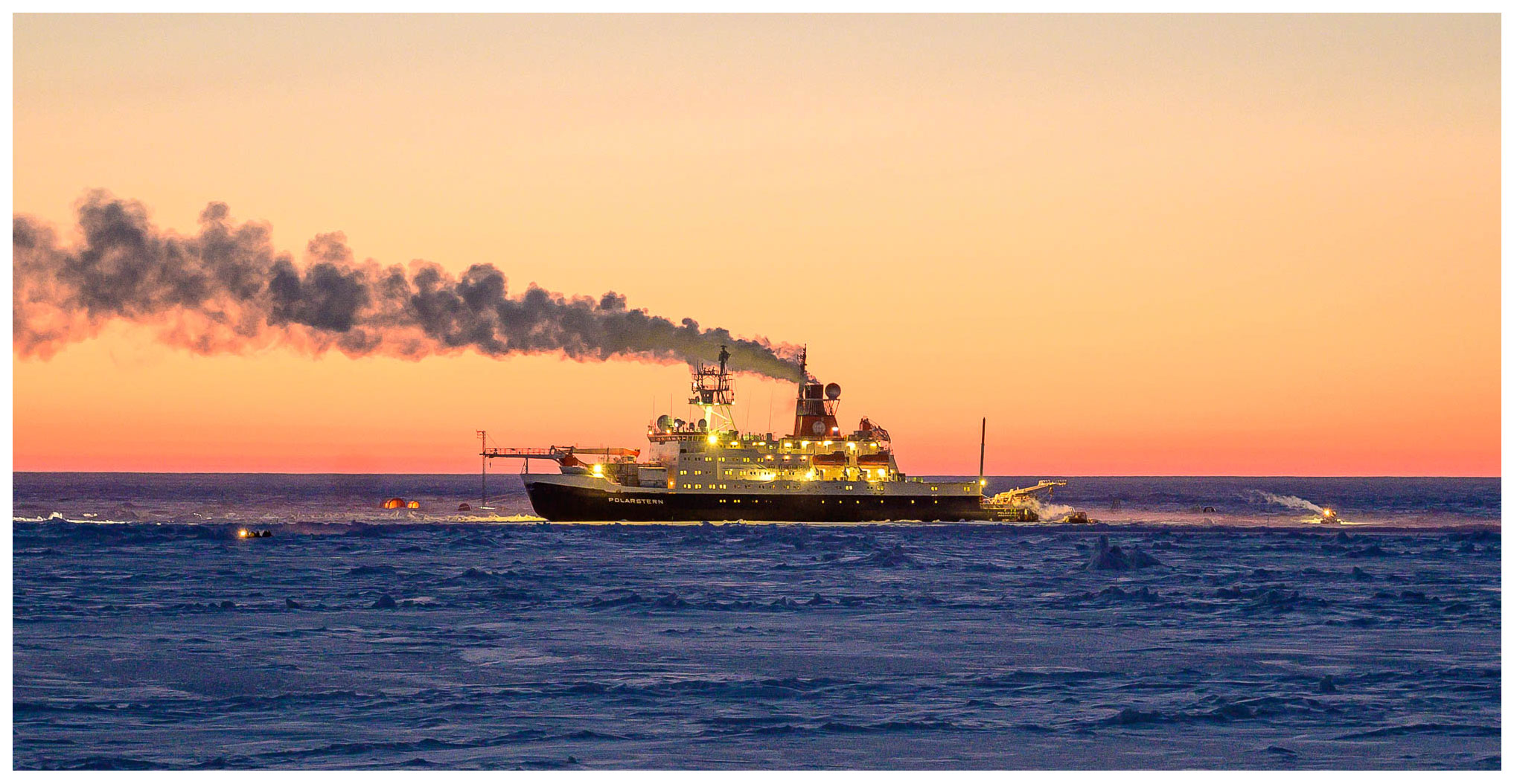
Figure A5 A situation when the wind was coming from the stack's direction and the exhaust plume went directly over the Swiss Container, but due to the surface inversion no pollution spikes were measured in the Swiss Container. The container was located at the bow of the ship, below the crane (left-hand side in this picture). Photo credit: Ivo Beck.

Figure A6 Same as Fig. 4 but for another day (16 January 2020). Panels (a)–(c) show the original particle number concentration data in red, overlaid with the unaffected data in blue. The application of additional filters in panels (b) and (c) does not show an effect. Panel (d) shows the distribution of the particle number concentrations of the complete dataset in red after the application of the gradient filter as a black contour line and after the application of all filters of the PDA in purple.

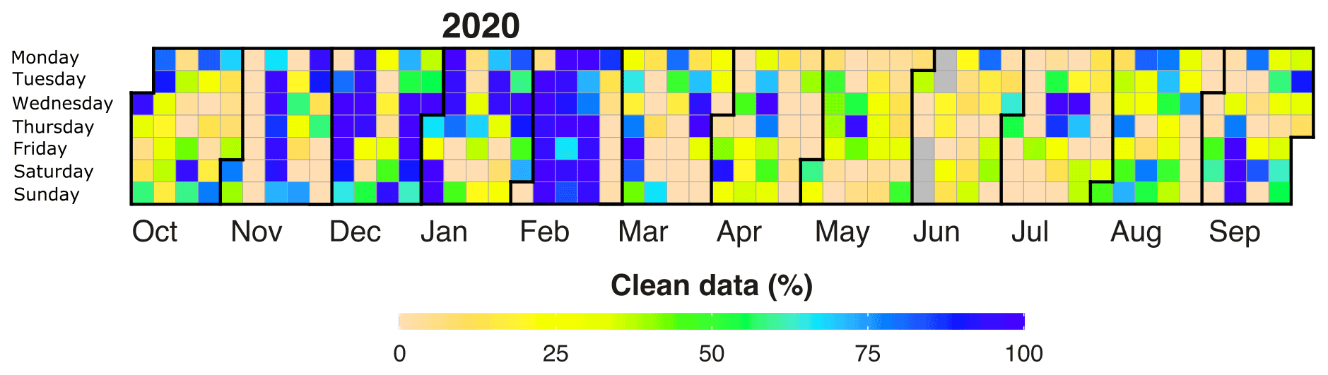
Figure A7 Percentage of clean particle number concentration data points per day during the MOSAiC expedition after application of the PDA. Missing data are indicated in gray and correspond to data removed when R/V Polarstern was within Svalbard's 12 nautical miles zone. Please note that this figure is indicative only and does not necessarily reflect the percentage of clean data points collected by other instruments during the expedition.

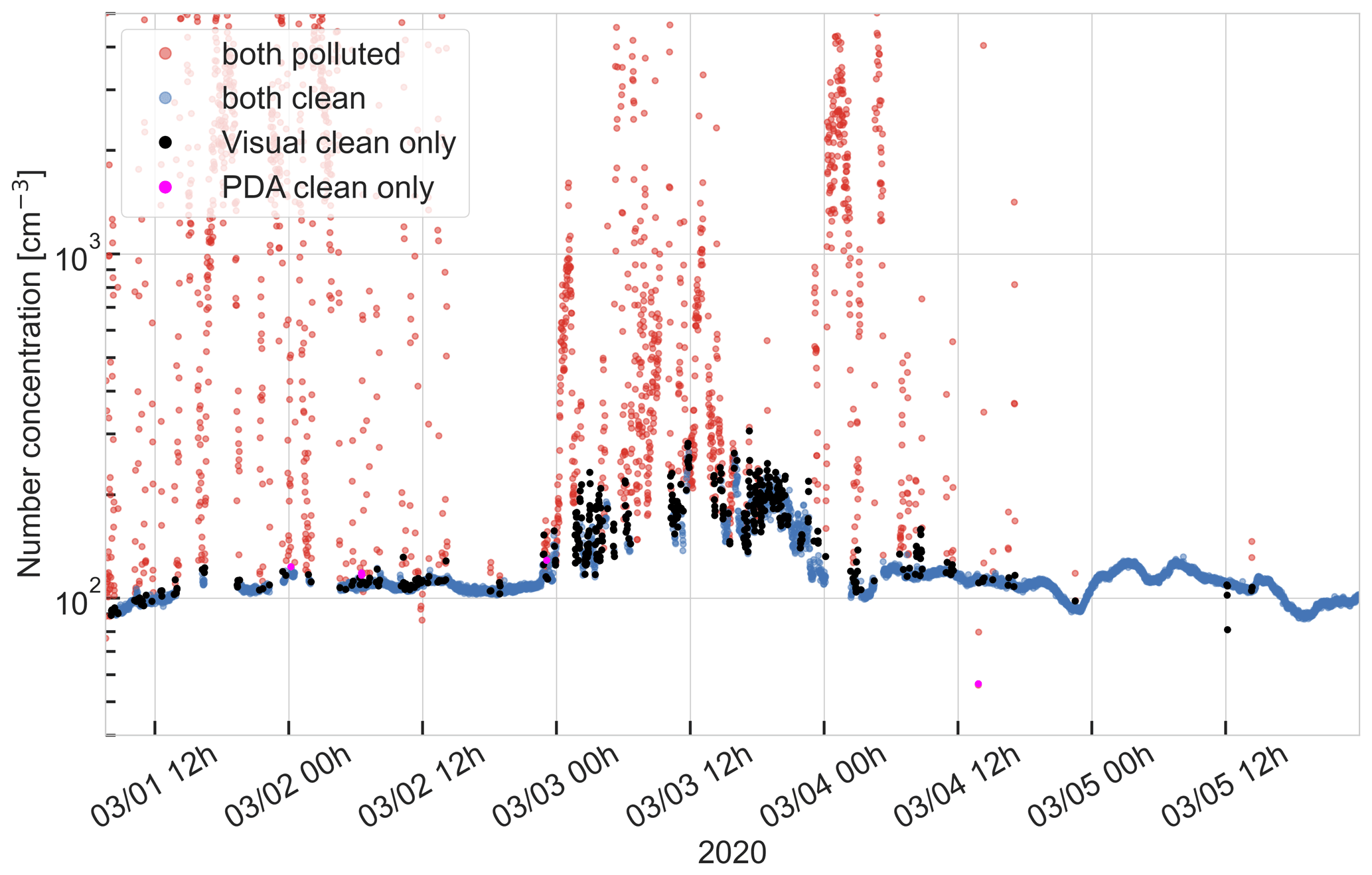
Figure A8 Time series with a comparison of the visual identification method and the PDA between 1 and 5 March. In red: data points which are detected as contaminated by both methods. In blue: data points which are detected as unaffected by pollution by both methods. In black: data points which are detected as unaffected by pollution only by the visual identification method. In magenta: data points which are detected as pollution free only by the PDA.

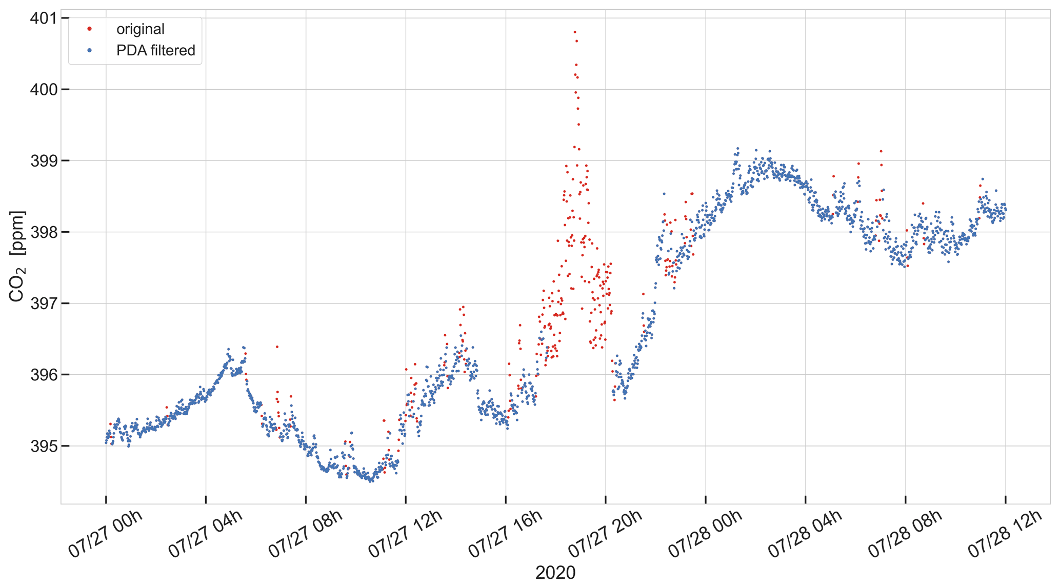
Figure A9 CO₂ mixing ratios on 27 July 2020 after the application of the PDA using step 1B. Original data are shown in red, overlaid with unaffected data filtered by the PDA in blue.

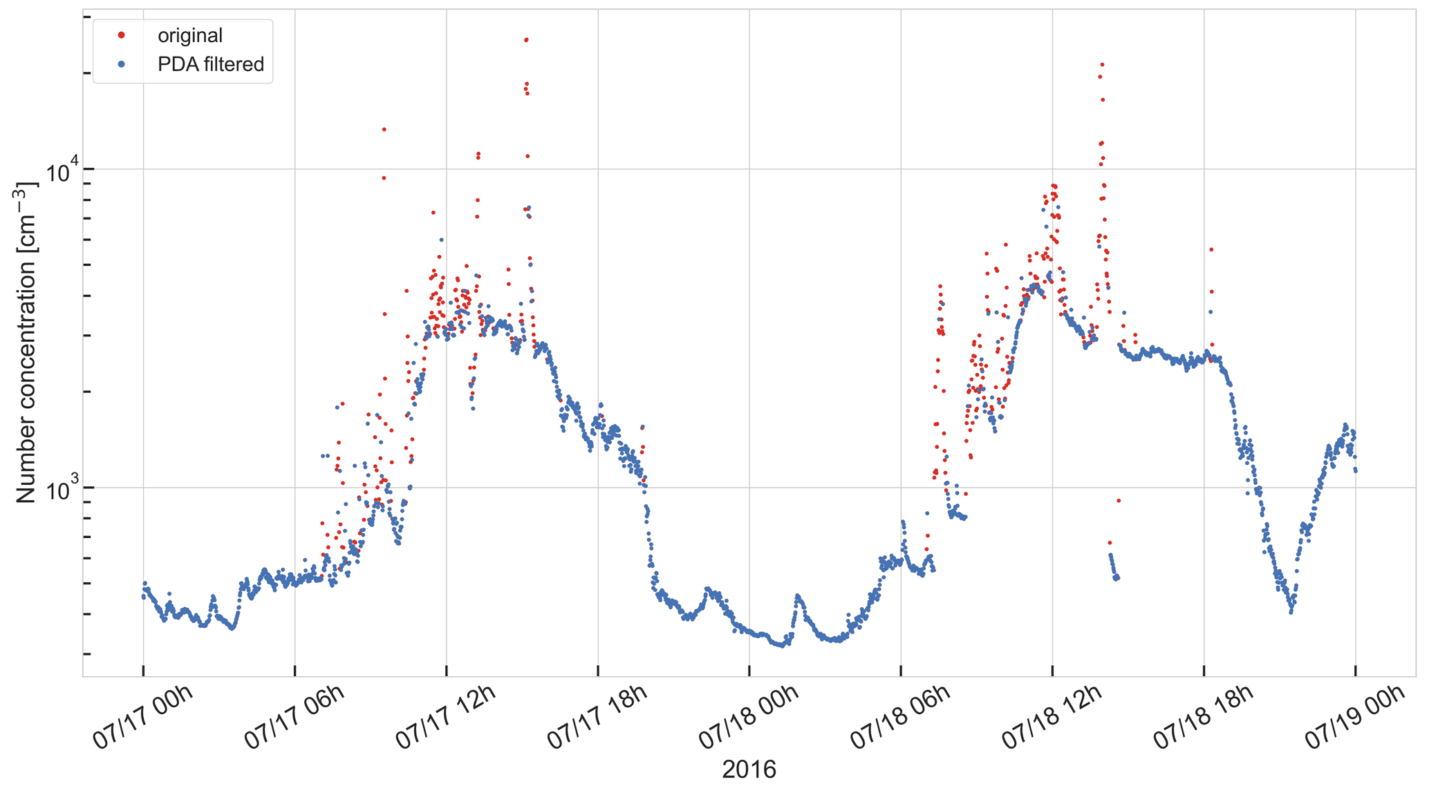
Figure A10 Time series of the particle number concentration dataset from JFJ after the application of the PDA. Original data are shown in red, overlaid with unaffected data filtered by the PDA.

Figure A11 Case study of 1 January 2020. The particle number concentration signal is influenced by contamination which shows as a noisy signal and not in distinct spikes. Panels (a)–(d) show the original particle number concentration data in red, overlaid with the unaffected data in blue after applying different filtering steps of the PDA. The orange circles highlight situations where applications of the neighbors filter and the sparse data filter improve the detection of polluted data significantly.

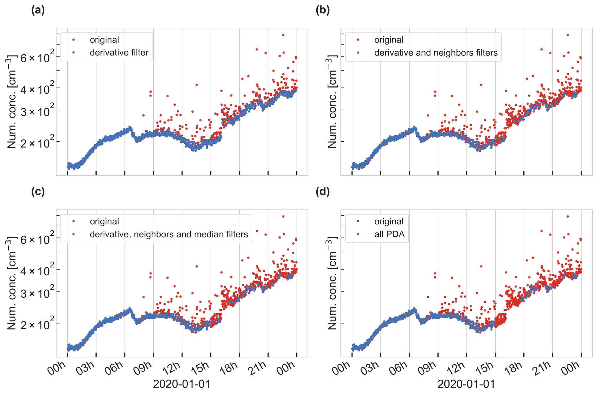
Figure A12 Same as Fig. A11 but with slightly stricter coefficients of the derivative filter. We chose a derivative filter with a=0.45 and m=0.5 to flag more data points in this case study.

Appendix B: Comparison of individual filtering steps

In Fig. B1, we compare how the application of each individual filtering step to the 1 min resolution dataset of the CPC3025 performs in the case study from 6 to 8 March. Panel (a) shows the result after the application of the derivative filter and the lower-threshold filter only (but not the upper-threshold filter) with a=0.5 and m=0.55 and a lower threshold of 60 cm⁻³. As we can see, the application of the derivative filter detects and flags most data points during the polluted time periods but leaves some during the contamination event on 6 March. The application of the derivative filter leaves 43 % of the data unaffected, and it reduces the mean concentration from 5198 to 202 cm⁻³. Panel (b) shows the application of the upper-threshold filter alone. Here we set the upper threshold to as low as 130 cm⁻³ to be able to retrieve the background signal as much as possible. With this threshold, 23 % of the data are left unaffected, with a mean concentration of 70 cm⁻³. However, the application of a single threshold to a longer time series is difficult, since the background concentration can rise to higher concentrations (as can be seen, for example, in Fig. 6). The upper threshold can be useful in cases when the measured concentration stays at the upper detection limit of the instrument over a long time period and thus the derivative filter would not catch those contaminated data points. Panel (c) shows the application of the median filter alone with a median window of 360 data points (6 h) and a median threshold of 1.05. The application of the median filter alone with these parameters leaves 68 % of the data unaffected, with a mean concentration of 2979 cm⁻³. It is not satisfying because it is not able to flag the strong contamination on 8 March after 12:00. Too many contaminated data points raise the median concentration. The median filter relies on a pre-cleaned dataset, where most of the contaminated data points have been removed already. Therefore, it can only be applied after the application of the derivative filter. Finally, panel (d) shows the result after the application of the whole PDA, with the parameters presented in Table 1. The application of the whole PDA leaves 38 % of the data unaffected, with a mean concentration of 191 cm⁻³. Evaluated visually by expert judgment, we find that it performs better than the application of the single filters, detects more contaminated data points, and results in a time series which represents the background concentration. Table B1 shows an overview of how many data remain unaffected after the application of the different filtering steps. Additionally, the mean concentrations and the standard deviations are shown. The derivative filter is by far the most powerful step of the PDA, as it already detects 64 % of the total contamination and reduces the mean concentration drastically. The other filters of the PDA only have a “fine-tuning” effect and add another 6 % of flagged data points. This effect can still be very important for individual cases, as shown in the case study on 6 March around 12:00 (Fig. 4).

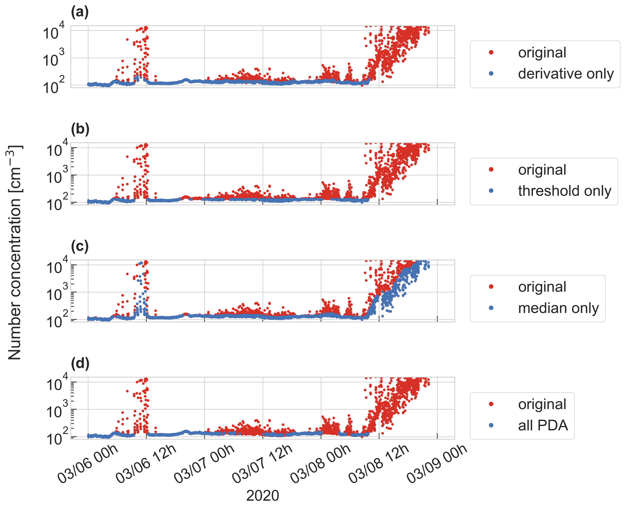
Figure B1 Intercomparison of individual filtering steps in a case study of 6 to 8 March. Clean data (in blue) are overlaid over the original data (in red) after the application of one filtering step individually to the data: the (a) derivative filter, (b) threshold filter, (c) median filter, and (d) all filtering steps of the PDA were applied. For all plots we used data from the CPC3025 at 1 min time resolution. Original data have only been pre-cleaned for zero filter measurements.

Figure B2 Power spectral density (PSD) of the particle number concentrations of the CPC3025 as a function of the frequencies. The dataset has a time resolution of 10 s. For this figure we used the subset of the month of March.

Since local contamination often shows in quickly changing concentration spikes, it is worth exploring whether a low-pass filter is applicable. For this, we looked at the power spectral density of the CPC3025 particle concentration data by means of a Fourier frequency decomposition (Fig. B2). No high frequency is visible which would allow a low-pass filter to be applied. Local contamination in this dataset does not show in a high-frequency signal, which is distinguishable from the background signal. The detection of pollution based on frequency analysis is therefore not possible here.

Table B1 Percentage of data declared as unaffected when different filtering steps are applied and the mean concentrations and standard deviations of the corresponding particle number concentrations.

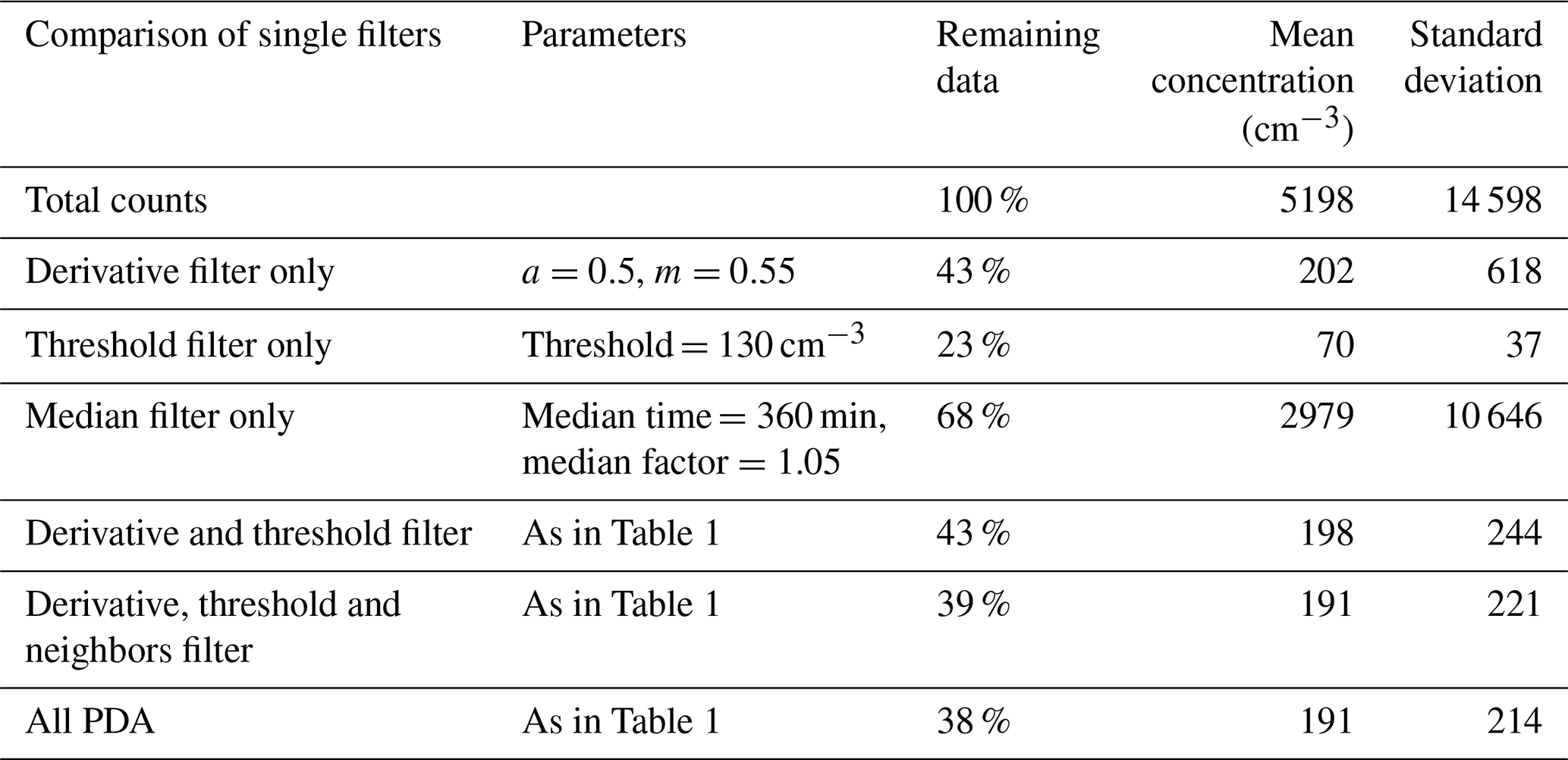
In order to elaborate on the effect of changes in the parameters of individual filtering steps, we let the PDA run several times and thereby only change one parameter at the time. The resulting size of the filtered dataset is shown in Table B2. The first row shows the initial setting as we used them in Table 1. For example, the largest change is caused by turning off the neighbors filter. This increases the dataset by 11.4 %. Relatively small changes in the power law slope and intercept of the derivative filter change the size of the dataset by roughly 5 % to 10 %, whereby the effect of changes in the slope are stronger. Changes in the median filter only cause small changes by <1 % to the final dataset, and setting the sparse threshold from 24 to 18 out of 30 data points (from 80 % to 60 % allowed polluted data points in the sparse window) reduces the dataset by ca. 3 %. The table illustrates again that the derivative filter is responsible for the largest part of the filtering by the PDA. Even though the filtering steps 2 to 4 only contribute little to the PDA, they are valuable for avoiding false negatives after the application of the derivative filter.

Table B2 The effect of changes in the parameters of individual filtering steps on the number of unaffected data points. The first row shows the standard settings used to filter the CPC3025 dataset and the number of remaining data points. The following rows show changes in different parameters and again the number of unaffected data points with these changes in the PDA.

Appendix C: Application of the PDA to various time resolutions

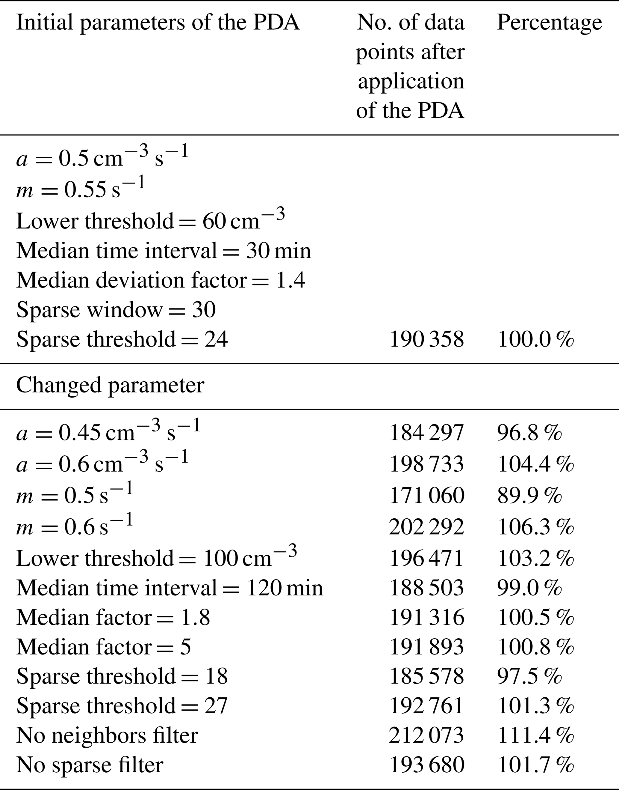
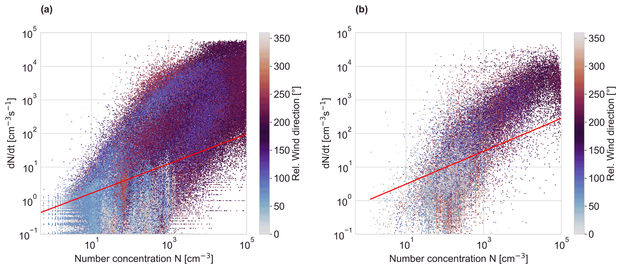
Figure C1 Relation of the absolute value of the particle number concentration derivative to the absolute number concentration for two different time resolutions: (a) 10 s; (b) 10 min. The color code indicates the relative wind direction. The red lines separate polluted from unaffected data points with a slope of 0.44 s⁻¹ and an intercept of 0.6 cm⁻³ s⁻¹ in panel (a) and a slope of 0.49 s⁻¹ and an intercept of 1 cm⁻³ s⁻¹ in panel (b).

We use the averaged time series from the derivative filter for further filtering steps in the PDA. This comes with the trade-off that the dataset loses time resolution when applying the PDA. In many applications this might not be a problem since data are often collected at higher time resolutions than needed for further analysis. We applied the PDA to the original dataset of the CPC3025 (10 s time resolution). Figure C1a shows the derivatives plotted against the total number concentrations for this dataset, which is used to determine the separation line (in red) for the derivative filter. It is less intuitive to find a good position of the separation line compared to the 1 min-averaged derivative (Fig. 3), because the two branches do not separate as clearly. We chose a separation line with the parameters a=0.6 cm⁻³ s⁻¹ and m=0.44 s⁻¹. Figure C1b shows the same graph for the 10 min-averaged time series of the same dataset. Here, we used a=1 cm⁻³ s⁻¹ and m=0.49 s⁻¹ for the separation line. In both cases, it is possible to distinguish between the two derivative branches, which indicates polluted and unaffected data. We observe that the separation line tends to go to higher derivatives with coarser time resolution, which is a result of the longer averaging time, because this smoothens the variability. Figure C2 shows the original (in red) and filtered (in blue) time series over 3 d after application of all PDA filtering steps to the two datasets (10 s time resolution in panel a and 10 min time resolution in panel b). The used parameters of the PDA are listed in Table C1. The PDA detects the polluted spikes in both cases and is able to separate clean and polluted data. Even though the lower time resolution data do not have as distinct pollution “spikes”, potential outliers could have been smoothened when averaging. We conclude that the possibility of “tuning” different parameters of the PDA makes it applicable to datasets with different temporal resolutions.

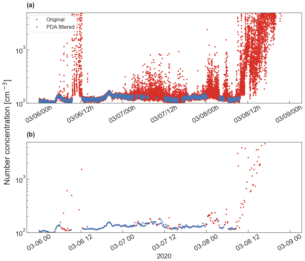
Figure C2 Performance test of the PDA on datasets with two different time resolutions: (a) 10 s time resolution data; (b) 10 min time resolution data. Filtered data in blue are shown on top of the original data of the corresponding time series in red.

Table C1 Parameters used for the application of the PDA to two datasets with different time resolutions.