the Creative Commons Attribution 4.0 License.
the Creative Commons Attribution 4.0 License.
 | 21 Oct 2022
Source apportionment resolved by time of day for improved deconvolution of primary source contributions to air pollution
Sahil Bhandari
Zainab Arub
Gazala Habib
Joshua S. Apte
Present methodologies for source apportionment assume fixed source profiles. Since meteorology and human activity patterns change seasonally and diurnally, application of source apportionment techniques to shorter rather than longer time periods generates more representative mass spectra. Here, we present a new method to conduct source apportionment resolved by time of day using the underlying approach of positive matrix factorization (PMF). We call this approach “time-of-day PMF” and statistically demonstrate the improvements in this approach over traditional PMF. We report on source apportionment conducted on four example time periods in two seasons (winter and monsoon seasons of 2017), using organic aerosol measurements from an aerosol chemical speciation monitor (ACSM). We deploy the EPA PMF tool with the underlying Multilinear Engine (ME-2) as the PMF solver. Compared to the traditional seasonal PMF approach, we extract a larger number of factors as well as PMF factors that represent the expected sources of primary organic aerosol using time-of-day PMF. By capturing diurnal time series patterns of sources at a low computational cost, time-of-day PMF can utilize large datasets collected using long-term monitoring and improve the characterization of sources of organic aerosol compared to traditional PMF approaches that do not resolve by time of day.
- Article
(3530 KB) - Full-text XML
- Companion paper
-
Supplement
(2558 KB) - BibTeX
- EndNote


Air pollution is considered the greatest current environmental health threat to humanity, with an estimated mortality burden of 7 million per year (World Health Organization, 2018; Schraufnagel et al., 2019; Health Effects Institute, 2020). Air pollutants also cause climate forcing and environmental damages to ecosystems and biodiversity (Intergovernmental Panel on Climate Change, 2019, 2021). Apart from physiological and environmental effects, air pollution is associated with negative psychological, economic, and social effects (Lu, 2020). High race-, ethnicity-, income-, region-, and nationality-based disparities exist in air pollution exposure, making air pollution exposure an important environmental justice issue (Hajat et al., 2015; Goodkind et al., 2019; Tessum et al., 2019; Thind et al., 2019; Health Effects Institute, 2020; Pandey et al., 2020; Chakraborty et al., 2021). These disparities are associated with a wide variety of sectors, activities, processes, and pollutants (Thakrar et al., 2020). Policy solutions targeting specific pollutants have led to nonuniform reductions of air pollution contributions of different sectors (Tschofen et al., 2019). Thus, reduction of air pollution is essential to global health and can be expected to generate long-term societal benefits (Tessum et al., 2019; Goodkind et al., 2019; Tschofen et al., 2019; Organization for Economic Co-operation and Development, 2020). However, more than half the world's population is exposed to increasing air pollution (Shaddick et al., 2020). Most of this population lives in developing nations. Moreover, economic resources are limited, and reduction of air pollution alongside continued economic growth requires investment in abatement measures for older technologies and adoption of cleaner technologies (Lei et al., 2021). Thus, sources of air pollution need to be prioritized to appropriately focus limited resources on the most effective abatement measures. This prioritization should be based on the contributions of different emission sources to air pollution in a region.
Source apportionment is the practice of attributing air pollution to different causes such as sectors (residential, industrial), activities (traffic, biomass burning), and atmospheric processes (oxidation). Several approaches have been developed to conduct source apportionment studies (Belis et al., 2014). Broadly, these approaches can be categorized into emission inventories, receptor-oriented modeling, and source-oriented modeling. These approaches have been accepted by regional, national, and international agencies for use in air quality policy and planning (Belis et al., 2014; Environmental Protection Agency, 2017; California Air Resources Board, 2018; Wayland, 2018). Source-oriented models and emission inventories together capture the emissions, chemical transformation, transport, and dispersion of pollution. However, they have heavy computational burden, require extensive data collection, and are subject to cumulative uncertainties from model inputs as well as the different computational components (Hopke, 2016). Receptor models are mathematical tools with relatively lower computational requirements that use mass balance analysis to output source contributions (time series of source concentrations) and source profiles (relative strength of different pollutants) for identified sources of air pollution (Belis et al., 2013; Hopke, 2016). Positive matrix factorization (PMF) has been identified as an appropriate receptor modeling technique that can be deployed for quantifying source contributions for air quality management (Belis et al., 2015).
Three tools are currently in active use for application of PMF to atmospheric datasets: the Igor PMF Evaluation Tool (PET) (Ulbrich et al., 2009), the EPA PMF tool (Brown et al., 2012), and Source Finder (SoFi) (Canonaco et al., 2013). The Igor PET tool uses the PMF2 program to resolve factors from 2-D matrices (Paatero and Tapper, 1994; Ulbrich et al., 2009). Further details on the statistical basis of this method are available elsewhere (Ulbrich et al., 2009; Zhang et al., 2011, and references therein). Both SoFi and EPA PMF are based on the Multilinear Engine (ME-2), which allows for the application of factor profile constraints to extract specific sources (Paatero, 1999; Paatero et al., 2002; Canonaco et al., 2013; Crippa et al., 2014; Norris et al., 2014). PMF2 does not allow for the application of factor profile constraints, and it often results in greater uncertainty in solutions, poorer source separation, and fewer identified sources compared to ME-2 (Ramadan et al., 2003; Amato et al., 2009; Amato and Hopke, 2012). A further important advantage of the EPA PMF tool over Igor PET and SoFi is its error estimation techniques, which systematically account for both random error and rotational ambiguity using bootstrapping, displacements, and bootstrapping enhanced with displacements, as explained in more detail in Sect. 2.5 (Paatero et al., 2014; Brown et al., 2015). Currently, the Igor PET and the SoFi tools only use bootstrapping to account for random errors and, partially, rotational ambiguity (Ulbrich et al., 2009; Canonaco et al., 2021).
PMF tools have been applied to identify sources using long-term datasets spanning multiple years (Zhang et al., 2019; Heikkinen et al., 2020) and seasonal datasets accounting for seasonal variability (Amil et al., 2016; Bikkina et al., 2019; Bhandari et al., 2020; Patel et al., 2021a), for studying special events (Reyes-Villegas et al., 2018; Rai et al., 2020, Patel et al., 2021b) and spatial variability (Crippa et al., 2014; Robinson et al., 2018), as well as for connecting sources to health effects (Daellenbach et al., 2020). Several studies have analyzed the influence of meteorology after conducting source apportionment on a larger dataset (Venturini et al., 2014; Pauraite et al., 2019; Bhandari et al., 2020). Some studies have quantified the effect of meteorological variables on the performance of the source apportionment approach for the identification of sources, with or without stratification. One such study stratified data based on mean temperature and showed that accounting for temperature variability using gas–particle partitioning before conducting source apportionment improved the stability of the solution (Xie et al., 2013a, b). Similar data-segmentation schemes have been deployed for wind direction, wind speed, and precipitation, and these techniques resulted in a larger number of and more representative PMF factors (Park et al., 2019).
A major limitation of PMF is the assumption of constant factor profiles throughout the modeling period – while the contribution of each factor is modeled to change over time, its profile (e.g., mass spectrum, when PMF is applied to mass spectrometer data) stays constant, which leads to modeling uncertainty (Ulbrich et al., 2009). Previous studies have tested the limitation of constant mass spectral profiles for seasonal and weekly changes in meteorology and activity patterns (Canonaco et al., 2015, 2021; Reyes-Villegas et al., 2016). These studies found that annual and seasonal datasets from an aerosol chemical speciation monitor (ACSM; Aerodyne Research, Billerica, MA) show high variations in mass spectral contributions, which cannot be sufficiently captured when PMF is conducted on the complete dataset. These studies recommended conducting PMF analysis on shorter time frames (weeks–months) with limited variability of emissions and meteorology. However, meteorological conditions influence source apportionment on hourly and smaller timescales; for example, changes in ventilation (Dai et al., 2020) and photochemistry (Lelieveld and Crutzen, 1991) affect source apportionment results. Human activity patterns also vary with time, leading to changes in source cocktails – for example, we expect higher cooking emissions during cooking-influenced periods (Abdullahi et al., 2013; Patel et al., 2021a), higher traffic emissions during rush hour (Zhang and Batterman, 2013), and time-of-day, day-of-week, and month-of-year patterns for other emission sources (Crippa et al., 2020). These changes in meteorology, photochemistry, and sources lead to diurnal variability in mass spectra (MS). For example, Canonaco et al. (2015) showed that the mass spectra of secondary organic aerosol (SOA) changed with concentrations of OX (O3 + NO2), which shows high diurnal variability due to monotonic association with ambient temperature. Finally, diurnal variability of time series patterns is frequently used for PMF factor selection and representation (Zhang et al., 2011). As an example, using data from 11 d of PMF runs, Williams et al. (2010) presented bi-hourly diurnal variability of PMF factor time series contributions. Recognizing the importance of variability of source influence at receptor sites, previous research has examined the influence of sampling periods, sampling time resolution, and time series variability of source emissions on the final PMF result (Tian et al., 2017; Wang et al., 2018). Results from these studies suggest that, given the assumption of constant factor profiles in PMF, PMF analysis should be conducted on time-resolved datasets. Additionally, to capture source emission and meteorological variability over the day, data from all times of day should be collected. Thus, an ideal PMF technique would make the most of the high time resolution of datasets while assuming constant factor profiles for periods with limited variability in emissions and meteorology.
One such approach is conducting different PMF runs for different times of the day across long-term datasets. A key advantage of such sub-setting is that it captures the diurnal variability in source apportionment using PMF while keeping computational load to a minimum. Differences in factor profiles between the seasonal PMF and time-of-day PMF runs may indicate the effect of diurnal process changes and/or reactivity (Norris et al., 2014). Conducting PMF on smaller time windows is expected to improve results for another reason. Positive matrix factorization approaches have influence functions that are designed to account for the influence of outliers on the solutions (Paatero, 1997; Paatero and Tapper, 1994; Ulbrich et al., 2009). These outliers depend on the time window on which the factorization is being applied (Paatero, 1997). A shorter time window for analysis is influenced by outliers present in that time window only and not any other period. Thus, a shorter time window can be expected to give higher factor resolution, given that the influence of many outliers in the dataset is removed. At the same time, the number of zeros in the dataset also assists with the quantification of PMF factors (Paatero, 1997). Thus, shortening time windows can also decrease the extraction of factors via PMF, as has been reported previously (Tian et al., 2017).
This paper improves upon the seasonal source apportionment previously employed in Delhi (Bhandari et al., 2020). The Delhi Aerosol Supersite (DAS) study provides long-term chemical characterization of ambient submicron aerosol in Delhi, with near-continuous online measurements of aerosol composition (Gani et al., 2019, 2020; Arub et al., 2020; Bhandari et al., 2020; Patel et al., 2021a). In that study (Bhandari et al., 2020), PMF was conducted on six seasons of highly time-resolved speciated nonrefractory submicron aerosol (NR-PM1) organic (Org) mass spectrometer data from an aerosol chemical speciation monitor (ACSM) in the PMF receptor model at a time resolution of 5–6 min. Then, we deployed the Igor PET tool on seasonal datasets, and two to three PMF factors were extracted. The extraction of a low number of factors implies low rotations, and therefore quantitative error estimation was not conducted in that study (Paatero and Tapper, 1994).
Here, we apply the approach of conducting PMF on long-term datasets where each day was separated into six 4 h periods with limited variability in emissions and meteorology. To our knowledge, no study has systematically assessed the use of PMF on data resolved by time of day. In this paper, we report on PMF conducted on ACSM organic aerosol data from the winter and monsoon seasons of 2017 – collected as a part of the Delhi Aerosol Supersite (DAS) study – after resolving by time of day. Thus, the factor MS are expected to vary in these time-of-day windows. The winter and monsoon seasons are selected for this analysis as they capture two extremes in seasonal concentrations, precipitation, and meteorology, especially in terms of temperature, ventilation coefficient, wind direction, and wind speed (Tables S1 and S2 and Fig. S1 in the Supplement). In addition, winter experiences extremely high organic and inorganic concentrations and high pollution episodes dominated by primary emissions (Gani et al., 2019; Bhandari et al., 2020). We use the EPA PMF tool to apply constraints, extract a larger number of factors, and quantify errors in PMF solutions.
2.1 Statistical basis of approach
ME-2 is a multilinear unmixing model that can be used to perform bilinear deconvolution of a measured mass spectral matrix (X) into the product of positively constrained mass spectral profiles (F) and their corresponding time series (G), as shown in Eq. (1). In Eq. (1), E corresponds to the data residual not fit by the model. Given that time series and mass spectra are deconvoluted, the model mass spectral profiles are assumed to remain constant in time. The mass balance equation underlying the bilinear implementation of the factor analytical model and the optimization problem in the EPA PMF tool can be represented as shown in Eqs. (1)–(3).
Equation (2) is an elemental notation of Eq. (1). For ACSM data analyzed here, xij represents an element of the m×n data matrix X, where i represents a single time point, and j represents a measured ion or . n corresponds to the number of factors in the PMF solution. Thus, gip refers to the time series contribution of the pth factor at the ith time point, and fpj represents the mass spectral contribution of the jth in the pth factor profile.
To derive factor time series and mass spectra in an iterative fitting process, ME-2 lowers the residual by minimizing the quality-of-fit parameter Q, using the gradient approach (Norris et al., 2014; Eq. 3). Thus, PMF attempts to achieve a global minimum for the optimization problem. Q is the weighted least-squares error (sum of squares of model error normalized to measurement error) or the summation of squares of scaled residuals of the fit at each data point. We do not expect the norm of the actual error matrix to be zero but instead close to the ACSM measured uncertainty (an element of the measured uncertainty is represented as σij in Eq. 3). The quality-of-fit parameter corresponding to this uncertainty is called Qexp (Ulbrich et al., 2009). While Qexp is precisely equal to mn, for large m and n, it simplifies to ∼mn. Usually, PMF solutions start from very high and converge to 1 as more factors are added. We refer to the Q for the entire dataset as Q0.
For this discussion, we assume that Eq. (3) is subject to a constant mass spectrum F0 and variable time series G0. A key limitation of PMF is that it assumes constant MS profiles, even though source signatures can change over the course of the day. To address this limitation, we divide our data into time segments to conduct PMF analysis resolved by time of day. We refer to this time-resolved organic MS-based PMF as “time-of-day PMF” and the traditional approach as “seasonal PMF” in the paper. In the time-of-day PMF approach presented here, we minimize Q separately in each of these time-of-day windows.
2.2 Mathematical formulation of the time-of-day PMF approach
The mathematical formulation of the time-of-day PMF approach is introduced in Eqs. (4)–(17). To provide an example for splitting of data by time of day, we modify Eq. (3), dividing the data matrix X into Xday (time, t∈ [00:00, 12:00]) and Xnight (time, t∈ [12:00, 00:00]) (Eq. 4). Here, we demonstrate that splitting the data by time of day will result in a better solution. Thus,
The mathematical representation of the objective functions for conducting PMF separately for Xday and Xnight periods is shown in Eqs. (5) and (6) respectively. We call Q for these data subsets Q1 and Q2.
For this discussion, we assume that Eq. (5) is subject to a constant mass spectrum F1 and variable time series G1 for dataset Xday, and Eq. (6) is subject to a constant mass spectrum F2 and variable time series G2 for the dataset Xnight. For simplification,
Using these definitions, we can also redefine Q0 as shown in Eq. (10).
Clearly, Q0 minimizes the sum of two functions A and B. Thus, Q0 is a multi-objective optimization problem attempting to achieve a global minimum for the combined dataset X (Gunantara and Ai, 2018; Eq. 10). The two functions A and B are globally minimized separately at (F1, G1) in Eq. (5) and at (F2, G2) in Eq. (6), respectively. Thus, by definition, Eqs. (5) and (6) can be written as
Adding the inequalities in Eqs. (11) and (12), we get
Since this is true for all (F, G), this is also true for (F, G) that gives the minimum of A+B. Thus,
In Eq. (16), Q and Q are Q contributions to Q0 in the (F, G) space corresponding to Q1 and Q2 respectively. Thus, we can see that if solutions to Q0 will attempt to minimize error in the (F, G) space corresponding to Q1 (minimize Q, the obtained solution will likely worsen the error in the (F, G) space corresponding to Q2 (and therefore not minimize Q. This property of solutions to multi-objective optimization problems is inherent to a large class of solutions known as Pareto solutions, which are used for source apportionment and air quality planning (Gunantara and Ai, 2018; Angelis et al., 2020). This limitation can also be viewed as a limitation on the mass spectral profiles – Q0 assumes constant mass spectral profiles for both day and night periods and likely fits both periods worse than the scenarios of Q1 and Q2, where separate mass profiles for the two periods were developed. Thus, in the traditional approach, varying time series (TS) on non-varying MS can only capture changes as a linear TS scaling factor for all MS contributions. In the time-of-day PMF approach, both MS and TS vary, and we can expect new MS and TS patterns. For the special case of the day–night data split, where an equal number of points are collected in Xday and Xnight, Qexp (∼mn) corresponding to the two matrices is equal (we call it Qexpdn), whereas Qexp corresponding to the matrix X would be double that value (2 ). Using these values, Eq. (16) can be written as
Clearly, using the day–night split, we show that the sum of Q1 and Q2 (and the equivalent sum in ) would be lower than Q0 (and the equivalent sum of components). By inference, dividing the time series into periods of similar length (six 4 h segments in this paper) should result in a similar relationship as Eq. (17). Overall, conducting PMF on each such time-of-day period challenges the assumption of diurnally non-varying MS factors in typical PMF.
Table 1Summary of meteorology in the time-of-day PMF periods.
∗ Median values for ventilation coefficient (VC) and planetary boundary layer height (PBLH) are reported in parentheses. T – temperature, RH – relative humidity, WS – wind speed, and WD – wind direction.
2.3 Sampling site and measurements
As a part of the DAS study, an ACSM (Aerodyne Research, Billerica, MA) was operated at ∼0.1 L min−1 at ∼1 min time resolution in a temperature-controlled laboratory on the top floor of a four-story building at IIT Delhi (Ng et al., 2011b). Additionally, BC, ultraviolet-absorbing particulate matter (UVPM), and their difference ΔC were measured using a seven-wavelength aethalometer operated at the 1 L min−1 flow rate and 1 min time resolution (Magee Scientific Model AE33, Berkeley, CA) (Drinovec et al., 2015). These instruments were on separate sampling lines, both of which had a PM2.5 cyclone followed by a water trap and a Nafion membrane diffusion dryer (Magee Scientific sample stream dryer, Berkeley, CA). Full details of sampling site, instrument setup, operating procedures, calibrations, and data processing are described in a separate publication (Gani et al., 2019).
We collected the data used in this paper in winter (January–February 2017) and the monsoon (July–September 2017). Definition of the seasons comes from the Indian National Science Academy (2018) (Table 2 from Bhandari et al., 2020). Diurnal plots of meteorological variables are shown in Fig. S1. We conduct seasonal PMF runs for the winter and monsoon seasons of 2017 and time-of-day PMF runs for two periods (11:00–15:00 and 23:00–03:00 LT) in the two seasons. We used the dataset obtained by averaging every five consecutive measurements for the seasonal PMF runs. We selected organic spectral data at a specific set of values between 12 and 120. This approach is the commonly used approach, and the reasons for the selection of the specific set of values have been described previously (Zhang et al., 2005). Spring, summer, and autumn (mid-September to November) periods are not included in the analysis here, but seasonal PMF analysis has been presented in previous publications (Bhandari et al., 2020; Patel et al., 2021a).
2.4 PMF tool and runs
Here, we used two alternative approaches for conducting PMF. In one approach, we apply PMF by splitting the data into six 4 h time windows each day to illustrate the use of our time-of-day PMF method. The choice of the 4 h window was based on a preliminary PMF analysis conducted in the monsoon that allowed us to identify the influence of cooking organic aerosol, based on the ratio of contributions at 55:57 (Robinson et al., 2018). We started from 12 h time windows and kept decreasing the window size until the ratio was substantially greater than 1.6, suggesting the presence of a cooking organic aerosol (COA) factor in at least one such time window (in this case, it was monsoon 23:00–03:00 LT; Table 2). We also conduct seasonal PMF runs for the winter and monsoon seasons of 2017 and time-of-day PMF runs for two periods (11:00–15:00 and 23:00–03:00 LT) in the two seasons. Thus, we conduct four time-of-day PMF runs in total. The two time-of-day periods in each season are selected to differentiate between the influence of primary sources, changing MS due to reaction chemistry, and the effect of meteorology (Table 1, Fig. S1). As shown in the companion paper, these periods represent the two extremes in total NR-PM1) concentrations (Tables 1–2, Bhandari et al., 2022). Results from PMF analysis for all times of the day are presented in a companion paper (Bhandari et al., 2022), and a brief summary of those results is also provided in the Supplement of this paper (Sect. S5). In the monsoon and winter, traffic is expected to be a dominant source at night due to low cooking-related emissions and overlap with high nighttime traffic on major traffic corridors (Mishra et al., 2019). At midday in the monsoon, high temperatures and solar flux imply high photochemical processing of aerosols; therefore, we expect to see more oxidized aerosols (Table 1, Fig. S1). At winter in the nighttime, biomass burning for heating is an expected source. To refer to PMF runs corresponding to specific time windows, we use the nomenclature “season” + “period” in the format “S-TT-TT” (Table 1). For example, W-11-15 corresponds to 11:00–15:00 LT of winter 2017. Using data presented in this paper, we also compare the Q (and ) values from the seasonal PMF runs corresponding to the periods of the time-of-day windows (Sect. 3.5). While this work addresses the diurnal variations in MS patterns, future work could investigate the optimal length of the time window to sufficiently represent the finer diurnal variations (less than 4 h) in mass spectral profiles while managing computational burden.
The EPA PMF v5.0 tool was used to conduct ME-2 analysis on this dataset and interpret its results (Norris et al., 2014). Further details on the statistical basis of this method are available elsewhere (Paatero, 1999; Paatero et al., 2002). For the base run, the iterative PMF technique does not make any assumptions for source or time profiles. If factors extracted in the base run were not clearly associated with a source type but suggestive of the presence or mixing of specific sources, constraints were applied on the factors in the base run to extract cleaner source profiles (Brown et al., 2012, 2015). An R package was developed to automate the process of data analysis of EPA PMF outputs (R Core Team, 2019). We readjusted the results from PMF analysis to account for underestimation of factor mass based on the selected values only. To account for particle losses, we applied transmission and collection efficiencies after conducting PMF analysis (Gani et al., 2019).
Details of the steps for conducting PMF, R code, and criteria for factor selection are discussed in detail in the Supplement (Sect. S1). Briefly, for selection of PMF solutions, we started by analyzing the different statistics of (a measure of fit), correlogram of residual TS and correlation with external tracers, time series patterns in residuals, and PMF fits at different s (Table S4). We also considered the correlation of factor mass spectral profiles with reference mass spectra since MS of different factors are characterized by different spectral signature peaks (Zhang et al., 2011). For example, hydrocarbon-like organic aerosol (HOA) is a proxy for fresh traffic and combustion emissions and shows prominent peaks at values 55 and 57 and a higher fractional organic signal at 43 than 44. For separation of cooking organic aerosol (COA) and to distinguish it from HOA in this study, we used the Robinson et al (2018) ratio of contributions at 55:57 of 1.6 as a preliminary test for relative positioning of the HOA and COA profiles (COA factors with the ratio close to or greater than 1.6 and HOA profiles with the ratio substantially lower than 1.6). We also validated obtained PMF factors by correlation of factor time series with external tracers. We use two tracers for HOA influence: CO and the fossil-fuel component of black carbon, BCFF, estimated using the model of Sandradewi et al. (2008). For the time series of biomass burning organic aerosol (BBOA) factors, we use three tracers: (i) chloride (under the influence of agricultural and other open-waste-burning-related contributions (Li et al., 2014a, b; Kumar et al., 2015; Fourtziou et al., 2017); (ii) ΔC, defined as the difference between UVPM (370 nm) and BC detected by the aethalometer (Wang et al., 2011; Olson et al., 2015; Tian et al., 2019); and (iii) the biomass-burning component of black carbon, BCBB, estimated using the model of Sandradewi et al. (2008). COA-related factors often exhibit weak correlations with external tracers (Huang et al., 2010; Sun et al., 2011, 2013; Liu et al., 2012; Hu et al., 2016; Stavroulas et al., 2019). Additionally, the EPA PMF tool provides detailed uncertainty analysis tools to validate how representative the chosen PMF solutions are of the respective time windows. Here, we use the uncertainty analysis to select PMF solutions and only finalize solutions that pass the EPA PMF tests of random error and rotational ambiguity, as described below in Sect. 2.5. The application of these detailed uncertainty analyses to select a PMF solution for each time window, including the consideration of three- to eight-factor solutions, is documented in Table S6, with supporting information in Tables S5 and S7–S10.
2.5 Uncertainty estimation
In EPA PMF, quantitative error estimation (EE) of random error and rotational ambiguity was conducted using bootstrapping (BS), displacement (DISP), and bootstrapping enhanced with displacement (BS-DISP). This detailed uncertainty analysis ensures that the identified MS and TS are representative of the 4 h time windows by fitting hundreds to thousands of PMF-like model runs to data subgroups within the 4 h time windows (Paatero et al., 2014). Detailed summary statistics from running these uncertainty analyses are presented as mappings onto the PMF solution for the entire time domain (Tables S8–S10). The algorithms and computational workload of these techniques are described in detail elsewhere (Paatero et al., 2014). The application of these EE techniques leads to several orders of magnitude increase of computational time and memory requirements in conducting PMF runs (Paatero et al., 2014).
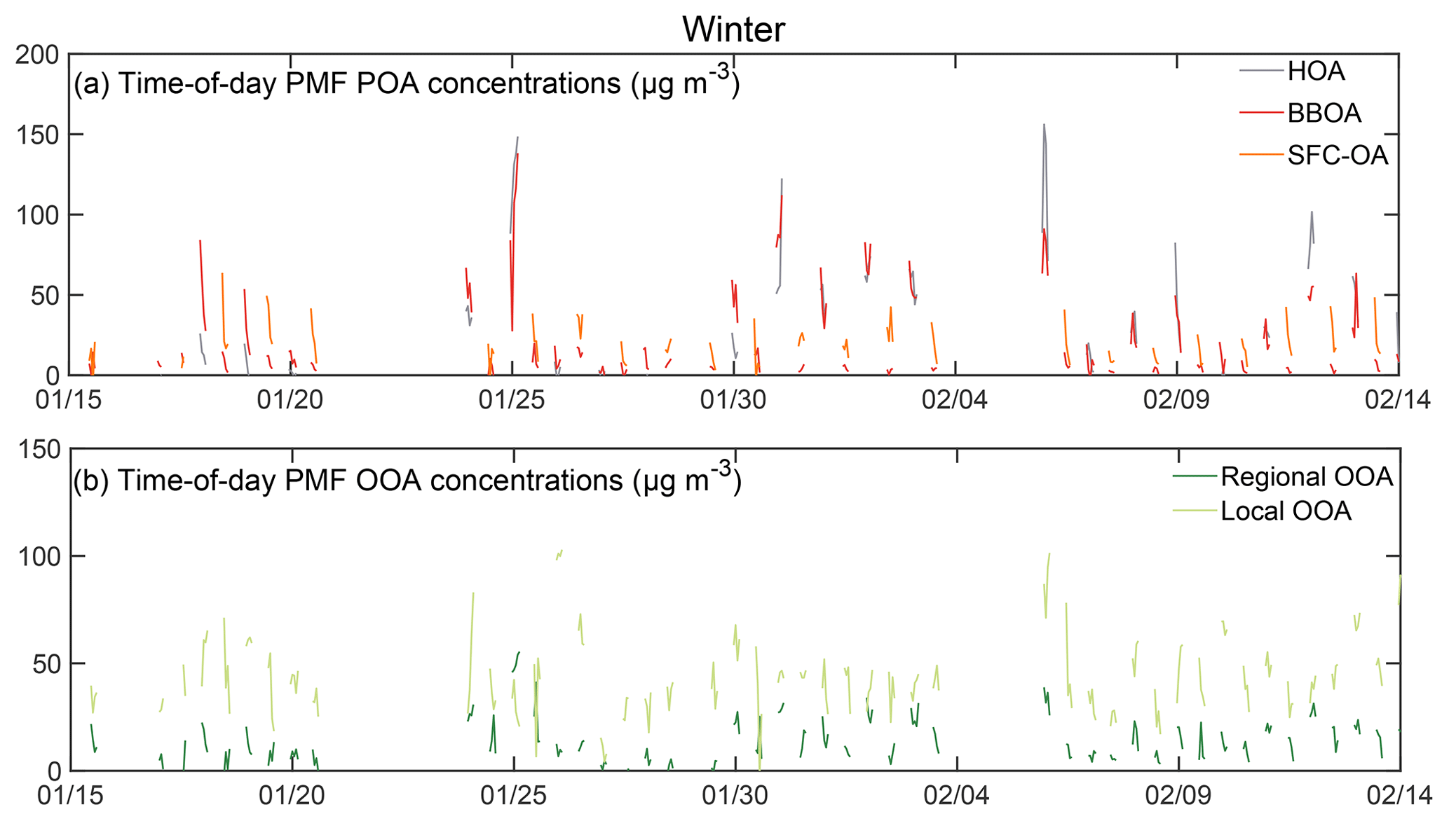
Figure 1Hourly averaged seasonally representative concentration time series of time-of-day PMF (a) primary and (b) secondary factors for winter 2017 (in µg m−3). POA PMF factors show stronger variability than OOA PMF factors. (Chopped lines are due to the analysis conducted on two 4 h periods each day.)
Bootstrapping or BS estimates “disproportionate effects of a small set of observations on the solution”. In the process, BS accounts for random error and to a limited extent rotational ambiguity (Norris et al., 2014). EPA PMF automatically identifies BS datasets using the parameter “block size” that is based on the principle of stationarity and accounts for underlying serial correlations (Politis and White, 2004). The default calculation of the “block size” in EPA PMF is based on incorrect calculations, and updated calculations have been published (Patton et al., 2009) but not implemented in the EPA PMF tool. We used the corrected block size estimation procedure as shown in the Supplement (Sect. S2, Table S5). BS factors are then mapped to base factors using the parameter “minimum correlation R value”, which is the minimum Pearson correlation coefficient used for BS factor assignment. We use the default value of 0.6 and conduct 100 BS runs for each PMF solution. Specification of too many factors in the base model may create artificial PMF factors (Ulbrich et al., 2009). BS factors with rotational ambiguity may also get mapped to other base factors. This scenario is called factor swapping and occurs for not-well-defined (NWD) solutions. These factors will likely have low BS mapping with their equivalent base run factors (Paatero et al., 2014). We only finalize PMF factor solutions with approximately 80 % or more BS mapping for all PMF factors.
Displacement or DISP estimates rotational ambiguity in PMF solutions by identifying the range of allowable MS profile contributions in the PMF factors. Bootstrapping enhanced with displacement or BS-DISP combines the bootstrap and displacement techniques to simultaneously estimate random error and rotational ambiguity in PMF solutions. In BS-DISP, BS resamples explore the solution space randomly, and DISP explores the rotationally accessible space around each BS resample. The ranges in DISP are obtained corresponding to four limits on changes in the Q value (dQ-max): 4, 8, 15, and 25. BS-DISP also reports ranges for contributions at different m/zs to MS profiles of PMF factors. These ranges correspond to four limits on changes in the Q value (dQ-max): 0.5, 1, 2, and 4. The obtained PMF factors using both approaches are then mapped to base factors, and the number of cases of factor swaps is noted. Sometimes, DISP and BS-DISP runs are terminated when encountering large changes in the Q value, which suggests the base case solution is not close to the global minimum. Generally, small changes in Q suggest PMF solutions are close to the global minimum. Additionally, a small number of factor swaps suggests low rotational ambiguity and robustness of the PMF solution. We only finalize PMF solutions with very few swaps at the smallest dQ-max value. Some DISP and BS-DISP runs terminated due to computational limits or encountering high dQ-max. For these cases, we used the number of factor swaps at termination as an estimate of total factor swaps. Finally, even when solutions with factor swaps are encountered, only solutions with swaps among the lowest number of factors are considered interpretable (Norris et al., 2014). All other solutions are rejected.
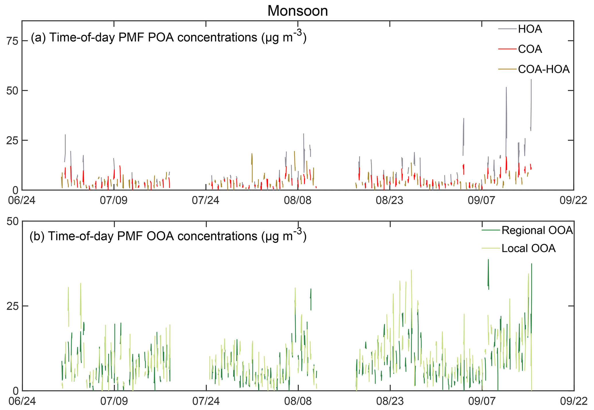
Figure 2Hourly averaged seasonally representative concentration time series of time-of-day PMF (a) primary and (b) secondary factors for the 2017 monsoon season (in µg m−3). POA PMF factors show stronger variability than OOA PMF factors. (Chopped lines are due to analysis conducted on two 4 h periods each day.)
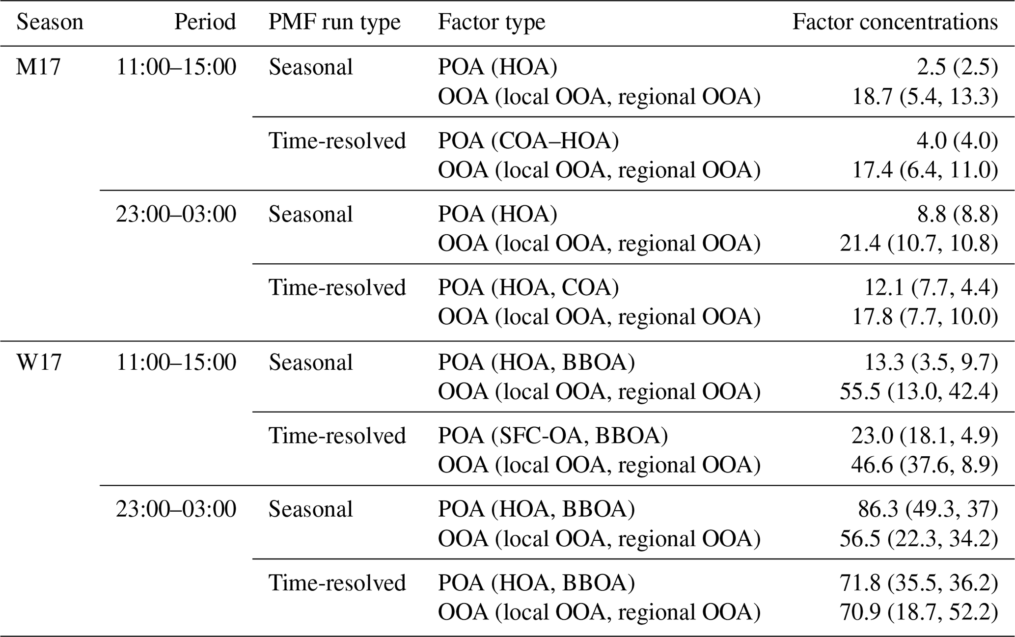
In this paper, we focus on the implementation of the time-of-day PMF technique on organic aerosol measured during monsoon midday and night periods and winter midday and night periods (Table 1). We report average concentrations of PMF factors in Table 2. For reference, data from seasonal PMF analysis are also presented. We find that time-of-day PMF analysis (i) generates a larger diversity of primary factors than seasonal PMF, (ii) resolves mass spectra of cooking-related factors such as cooking organic aerosol (COA), mixed COA–HOA, and solid-fuel combustion organic aerosol (SFC-OA) in Delhi, which are relatively unexplored (Tobler et al., 2020), and (iii) resolves different kinds of BBOA-related factors (two BBOAs, one SFC-OA) based on MS and TS correlations (Sect. 3.3) (Table 2). Seasonal monsoon PMF analysis represents primary organic aerosol (POA) by a single hydrocarbon-like organic aerosol (HOA), whereas monsoon time-of-day PMF analysis represents midday POA as a mixed COA–HOA factor and nighttime POA as separate HOA and COA. In winter, seasonal PMF analysis separates POA into HOA and BBOA factors. Winter time-of-day PMF analysis separates midday POA into an SFC-OA factor and a BBOA factor, and nighttime PMF analysis gives HOA and BBOA. All analyses generate two oxidized organic aerosol (OOA) factors. Time series of the different time-of-day PMF factors are shown in Figs. 1–2.
In Sect. 3.1, we discuss the mass spectral profiles (MS) and time series patterns (TS) of factors obtained in seasonal PMF analysis conducted for winter and monsoon. In Sect. 3.2, we discuss the mass spectral profiles and time series patterns of factors obtained in time-of-day PMF analysis conducted for winter and monsoon midday and nighttime periods. In Sect. 3.3, we contrast the mass spectra and time series patterns of primary and secondary PMF factors obtained from time-of-day and seasonal PMF analyses. The mass spectra of POA, a proxy for primary OA, and OOA, a proxy for secondary OA, were calculated by adding the component factors corresponding to each type (e.g., POA = HOA + BBOA + COA), weighted by their respective time series contributions. This estimation allows for a comparison between the results from the time-of-day and seasonal analyses. In Sect. 3.4, we compare the midday and nighttime POA and OOA MS profile results from the seasonal PMF and the time-of-day PMF approach. Our hypothesis is that the time-of-day PMF approach will show larger variability across the two time periods. In Sect. 3.5, we discuss period-specific Q (and ) values for the time-of-day PMF approach and the seasonal PMF approach. We also compare the TS patterns and by to identify periods and s with particularly significant changes in .
Table 2PMF factor concentrations in seasonal PMF and time-of-day PMF analysis (in µg m−3).
3.1 Seasonal PMF runs
The analysis in this section focuses on the PMF factors from seasonal PMF analysis; since this work focuses on specific times of day, the results are presented only for the 11:00–15:00 LT and the 23:00–03:00 LT time windows. Due to differing meteorology, sources, and photochemistry, the factor speciation, their mass spectra, and their time series patterns are quite different in the two seasons. A comparison of POA and OOA in different seasons has been previously presented (Bhandari et al., 2020). In winter, seasonal PMF analysis results in two factors representing POA, namely HOA and BBOA, whereas only HOA is obtained in monsoon seasonal PMF analysis. In the two seasonal PMF runs, we also obtain two OOA factors: local (less oxidized) OOA and regional (more oxidized) OOA (Drosatou et al., 2019; Table 2).
The behavior of the HOA factor MS is in line with the reference HOA factor MS, as suggested by the dominance of hydrocarbon signatures in the HOA spectrum belonging to the series CnH and CnH (Ng et al., 2011a; Bhandari et al., 2020; Pearson R∼0.95; Figs. S4, S5). In the monsoon, the seasonal PMF HOA MS is also strongly correlated with the reference COA factor MS (Ng et al., 2011a; Pearson R∼0.90; Fig. S5). However, the monsoon seasonal POA factor MS had a 55 to 57 ratio of 1.2 (Fig. S5). Therefore, the seasonal monsoon POA factor is presented as an HOA factor. This HOA factor has stronger correlations with tracers CO (Spearman R: 0.73) and BCFF (Spearman R: 0.91) than the OOA factors (Fig. S6). In winter, the fractional contributions of the BBOA factor MS at s 60, 73, and 115 are in line with the reference BBOA factor MS (He et al., 2010; Crippa et al., 2014; Bertrand et al., 2017; Pearson R∼0.90; Fig. S7). As expected, POA tracers, carbon monoxide (CO) and black carbon (BC), correlate more strongly with HOA and BBOA factor TS than with the OOA factor TS (Figs. S6 and S8). Additionally, BBOA correlates with chloride, particularly in the evening, suggestive of agricultural and other open-waste-burning-related contributions (Li et al., 2014a, b; Kumar et al., 2015; Fourtziou et al., 2017; Spearman R∼0.70; Figs. S8 and S9). We also observe strong correlations of the local OOA factor with chloride (Spearman R∼0.65; Fig. S8). These results are consistent with our previous seasonal organic–inorganic PMF analysis, which suggested that chloride, associated with an oxidized BBOA factor (likely a combination of local OOA and BBOA) with weak BCBB and ΔC correlations, might be linked to an industrial source (Bhandari et al., 2020). Indeed, chloride has weak correlations with BCBB (Spearman R∼0.45; Figs. S8 and S9).
OOA factors are principally associated with secondary organic aerosol (SOA; Zhang et al., 2011). Mass spectra of both local OOA and regional OOA correlate strongly with the reference OOA factor (Figs. S10–S11a, b; Pearson R≥0.95). However, local OOA correlates more strongly with the reference semi-volatile oxidized organic aerosol (SVOOA) factor (Zhang et al., 2011; Drosatou et al., 2019; Figs. S10 and S11; Pearson R∼0.80). The time series of the regional OOA factor correlates stronger with sulfate, whereas local OOA correlates stronger with chloride and black (BC) and brown carbon (UVPM) (Figs. S6 and S8). Overall, regional OOA shows less diurnal variability than local OOA, in line with a regional origin (Figs. S12 and S13). Detailed 15 min time series patterns of seasonal PMF factors for the midday (11:00–15:00 LT) and nighttime (23:00–03:00 LT) periods in the two seasons are discussed in the Supplement (Sect. S3).
3.2 Time-of-day PMF runs
The analysis in this section focuses on the PMF factors from time-of-day analysis for the 11:00–15:00 LT and the 23:00–03:00 LT time windows. Here, we show that time-of-day PMF analysis resolves mass spectra of cooking- and biomass-burning-related factors (one COA, one mixed COA–HOA, one SFC-OA, two BBOAs) based on MS and TS correlations. Only nighttime periods separate clean HOA factors.
3.2.1 Primary factor MS and TS
Winter 2017 primary factor MS
In winter at midday, PMF analysis results in two factors representing POA, SFC-OA and BBOA, whereas at nighttime, HOA and BBOA are obtained (Table 2). The behavior of the winter time-of-day PMF HOA factor MS is in line with the reference HOA factor MS (Ng et al., 2011a; Pearson R>0.95; Fig. S17a). The MS of the winter BBOA factors obtained are correlated with the reference profile but differ in contributions at key values such as s 29, 43, and 44 (Pearson ; Figs. S16b, S17b). Both MS profiles show much larger 29 contributions than the reference profile, suggesting a strong influence of wood burning (Bahreini et al., 2005; Schneider et al., 2006). The winter midday BBOA is more oxidized (MS shows a higher ratio of contributions at 44 to 43) and shows a low 60 contribution. It also has a high contribution at 15 (Fig. S16b). Similar BBOA MS profiles with high 15 have been observed previously as well (Crippa et al., 2013). In contrast, the winter nighttime BBOA is less oxidized, and BBOA MS show an 60 contribution closer to the higher end of the reference profile (Fig. S17b). At midday in winter, we also obtain a mixed POA factor (Fig. S16a). We call it solid-fuel combustion organic aerosol (SFC-OA) as the factor MS correlate with multiple reference MS profiles such as BBOA, HOA, and COA (Pearson R>0.8). This behavior is similar to a seasonal PMF SFC-OA factor identified recently in time-of-flight ACSM analysis for NR-PM2.5 in Delhi. In that study, that factor was expected to be associated with heating- and cooking-related domestic fuel combustion and open-fire activities (Tobler et al., 2020; correlation at all s but 44, Pearson R>0.95; Fig. S18).
Monsoon 2017 primary factor MS
At midday in the monsoon, we see only one POA factor, COA–HOA (Fig. S19). COA–HOA MS show similarities with both the reference COA and HOA MS (ref. COA: Pearson R 0.90, ref. HOA: Pearson R 0.80; Fig. S19). The inability to separate HOA and COA factors for mass spectral data obtained in a major city in the Indo-Gangetic Plain has been observed previously as well (Thamban et al., 2017; Bhandari et al., 2020). However, a key difference of this factor compared to the reference HOA and COA profiles is the large contributions at 44 in the monsoon midday COA–HOA. These high contributions are likely a result of the highly oxidizing environment in the afternoon. The afternoon overlaps with periods of high shortwave radiative flux (SWR) and therefore high reactivity of the atmosphere (Fig. S1). In the monsoon at nighttime, HOA and COA separate (Fig. S20a–b). The behavior of the monsoon nighttime time-of-day PMF HOA factor MS is in line with the reference HOA factor MS (Ng et al., 2011a; Pearson R>0.95; Fig. S20a). The monsoon nighttime COA factor MS are very similar to the reference COA factor MS (Pearson R 0.90; Robinson et al., 2018, ratio of contributions at 55 to 57–1.66; Fig. S20b). A key feature of this COA factor is the high 41, a characteristic feature of COA from heated cooking oils, especially in Asian cooking (Allan et al., 2010; Liu et al., 2018; Zhang et al., 2020; Zheng et al., 2020).
Primary factor TS
CO and BC serve as tracers for HOA, BBOA, and SFC-OA (Figs. S21–S24). The winter midday SFC-OA profile correlates strongly with chloride (Spearman R: 0.71), nitrate (Spearman R: 0.75), BCFF (Spearman R: 0.79), and ΔC (Spearman R: 0.60), pointing to the mixing of HOA, BBOA, and possibly COA in the factor (Fig. S21). In the winter at nighttime, we separate an HOA MS profile that correlates strongly with BCFF (Spearman R: 0.84) and CO (Spearman R: 0.83) (Fig. S22). We obtain one BBOA factor each for winter midday and winter nighttime. Among the two BBOA obtained, winter midday BBOA correlates strongly with chloride (Spearman R: 0.66) and CO (Spearman R: 0.67), suggesting an industrial source (Fig. S21, Sect. 3.1). At nighttime, however, winter BBOA correlates strongest with the wood burning component of BC (BCBB, Spearman R: 0.92) and weakly with chloride (Spearman R: 0.40), suggesting at least two different origins of BBOA (Fig. S22). This is consistent with our previous work, where we have separated BBOA-like factors with different correlations with chloride and BCBB in different seasons (Bhandari et al., 2020; Patel et al., 2021a). In the monsoon at midday, we observe only one primary factor, a COA–HOA factor, with strong correlations with chloride (Spearman R: 0.75), suggesting the influence of landfill emissions, trash burning, and solid-fuel sources (Fig. S23; Dall'Osto et al., 2015; Lin et al., 2017). Otherwise, COA–HOA has weak correlations with external tracers. Similar behavior of COA-dominated factors has been seen previously as well (Huang et al., 2010; Sun et al., 2011, 2013; Liu et al., 2012 Hu et al., 2016; Stavroulas et al., 2019). In the monsoon nighttime PMF run (M-23-03), we observe stronger correlations of the HOA factor with CO (Spearman R: 0.79) and BCFF (Spearman R: 0.86), compared to correlations of these tracers with the COA factor (CO: Spearman R: 0.70, BCFF: Spearman R: 0.71; Fig. S24).
3.2.2 Secondary factors' MS and TS
Time-of-day PMF and seasonal PMF generate two OOA factors, local OOA and regional OOA, in each run (Figs. S25 and S26). Typically, regional OOA is more oxidized (shows weaker correlations with reference SVOOA MS) and has less diurnal variation, in line with its expected average lower volatility and contributions from long-range transport (Drosatou et al., 2019). The time-of-day PMF OOA factors show MS and TS behavior similar to the seasonal PMF OOA factors, as shown in Sect. 3.3. Mass spectra of both local OOA and regional OOA correlate strongly with the reference OOA factor (Pearson R> 0.80; Figs. S25 and S26). Also, we consistently observe that the more oxidized regional OOA factors have flatter diurnal time series patterns (smaller range) than the less oxidized local OOA factors (larger range) (Figs. S27–S30; Table S11). However, we see an overlap of the 95 % confidence intervals of the normalized levels of the local and regional OOA factors (Figs. S27–S30) and an overlap of external tracers, suggesting mixing of the two OOA components (see Sect. S4). This is not surprising considering the similarity of MS of the two OOA factors and a continuum of the level of oxidation in the atmosphere (Drosatou et al., 2019). Since we observe factor mixing of the two secondary components, detailed analysis of the factor MS and TS (correlations with external tracers, features of the mass spectra) is only presented in the Supplement (see Sect. S4).
3.2.3 Time series patterns of time-of-day PMF factors
Time series patterns exhibit contrasting behavior in winter and monsoon time-of-day PMF analysis, similar to the seasonal factor contrast (Sect. S3; Figs. 3–4a, b). Midday concentrations of all primary factors exhibit a monotonically decreasing pattern, likely due to increasing ventilation (Figs. 3a, 4a, S1). In the midday period, winter peak SFC-OA and BBOA concentrations are both ∼3 times the period minimum (Fig. 3a). In the winter at night, peak concentrations of HOA and BBOA are ∼2.5 times and ∼3 times the period minimum (Fig. 3b). In contrast, monsoon primary factors exhibit lower variability at midday (peak COA–HOA concentrations∼2 times the period minimum) and nighttime (peak HOA ∼ 2.5 times the period minimum; peak COA ∼ 2 times the period minimum).
Additionally, the nighttime factors in both seasons show larger differences between the mean and the median than the corresponding midday factors in the same seasons, which suggests episodic nature of factors. The presence of episodes in these primary factors could be a consequence of the temperature-related inversions at nighttime, which lead to aerosol accumulation (Bhandari et al., 2020). These episodes could also be a result of episodic sources contributing to these factors. Generally, HOA shows the largest mean-median differences, and episodic contributions could be from heavy duty vehicles, brick kilns, and construction and road paving activities (Guttikunda and Calori, 2013; Dallmann et al., 2014; Mishra et al., 2019; Khare et al., 2020; Misra et al., 2020). For BBOA, these sources could be associated with burning events, as hypothesized previously (Bhandari et al., 2020). Episodic events could also be due to precipitation (Fig. S1). OOA factors experience mixing, so their time series patterns are not discussed.
Figure 3The 15 min averaged seasonally representative mean (+) and median concentrations (lines) of time-of-day PMF primary factors for the periods (a) W-11-15 and (b) W-23-03 (in µg m−3). Nighttime factors show evidence of episodes.
3.3 Comparisons of POA and OOA MS and TS obtained using time-of-day PMF and seasonal PMF
Results from the previous sections show that time-of-day PMF analysis generates a larger diversity of factors compared to seasonal PMF analysis. In this section, we summarize and compare the primary and secondary MS and TS contributions of factors using PMF results from two approaches – seasonal PMF and time-of-day PMF analysis. We show that (i) seasonal PMF analysis significantly underestimates primary concentrations at midday compared to time-of-day analysis (Tables 2 and 3; Figs. 5–6a, b); (ii) midday shows cleaner signatures in the POA factor MS in time-of-day PMF analysis compared to the seasonal PMF analysis (Figs. 7–8a, b); and (iii) nighttime OOA MS and TS show larger differences between the two techniques than nighttime POA MS and TS, whereas midday shows larger differences in POA MS and TS than OOA MS and TS (Table 3, Figs. 7–8a, b, S31–S36). Detailed MS and TS comparisons of time-of-day PMF POA and OOA with the seasonal PMF results are discussed below.
Figure 4The 15 min averaged seasonally representative mean (+) and median concentrations (lines) of time-of-day PMF primary factors for the periods (a) M-11-15 and (b) M-23-03 (in µg m−3). Nighttime HOA shows stronger episodes than COA.
Table 3Time series correlations of time-of-day POA and OOA TS with seasonal POA and OOA TS.

Here, we show that the time-of-day PMF approach shows strong similarities in time series patterns of primary factors compared to seasonal PMF analysis. However, the two approaches show substantial time-of-day-dependent differences in detected mass spectra.

Figure 5The 15 min averaged seasonally representative diurnal mean (+) and median (lines) concentration time series of POA for the periods: (a) W-11-15 and (b) W-23-03 (in µg m−3). Nighttime factors show evidence of episodes.
3.3.1 Comparison of POA time series
The behavior of POA is consistent with the individual component primary factors. POA is monotonically decreasing in all periods, concentrations are more variable during the day, and nighttime concentrations are several times those of midday concentrations (Figs. 5–6a, b). We observe striking similarities of the 15 min averaged time series patterns of POA between the two techniques across all periods (Table 3, Pearson R>0.85). The strong linear correlations suggest that time-of-day PMF analysis results in shifted (but correlated) TS patterns.
3.3.2 Comparison of POA mass spectra
The time-of-day PMF approach generates POA mass spectra both similar and different from the seasonal PMF approach, depending on the time of day (Figs. 7–8a, b). Two features stand out in these comparisons: the midday POA MS are dissimilar at key s, whereas the nighttime POA MS are nearly identical.
Figure 6The 15 min averaged seasonally representative diurnal mean (+) and median (lines) concentration time series of POA for the periods (a) M-11-15 and (b) M-23-03 (in µg m−3). Nighttime factors show stronger evidence of episodes.
Figures 7–8 show the MS pattern of time-of-day PMF POA and seasonal PMF POA for winter midday and nighttime (Fig. 7a–b) and monsoon midday and nighttime (Fig. 8a–b). In time-of-day PMF POA presented here, we observe a lower ratio of contributions at 43 to 44 than seasonal PMF POA. This lower ratio is indicative of the more oxidized nature of the POA factor compared to the seasonal POA (Ng et al., 2010). At midday, we observe higher contributions in time-of-day PMF POA at 44, in line with the high photochemical processing (SWR flux, Fig. S1). We also observe a higher ratio of contributions at 55 to 57 and lower contributions at 57 (Figs. 7a and 8a). These observations are in line with a strong cooking influence (and lower traffic influence) at midday (Ng et al., 2011a; Robinson et al., 2018). In winter at midday, we also observe lower contributions at s 29, 60, and 73 in time-of-day PMF than seasonal PMF (Bahreini et al., 2005; Schneider et al., 2006). This observation is likely a consequence of the removal of the influence of wood burning for nighttime heating on the time-of-day PMF POA MS for midday, in contrast to the seasonal PMF POA MS which are affected by the nighttime heating. In the monsoon at midday, we observe a higher contribution at 41 than 43 in time-of-day PMF POA, which is indicative of the influence of cooking (Allan et al., 2010; He et al., 2010). This POA also shows a higher contribution at 29, suggesting a higher influence of wood burning, likely associated with midday cooking. At nighttime, the differences between the time-of-day and seasonal profiles are much smaller. Overall, time-of-day PMF analysis seems to capture very specific features of primary aerosol behavior better than seasonal PMF analysis.

Figure 7Mass spectra of time-of-day PMF POA and seasonal PMF POA for the periods (a) midday and (b) nighttime in winter 2017. Midday MS show larger differences compared to nighttime MS.

Figure 8Mass spectra of time-of-day PMF POA and seasonal PMF POA for the periods (a) midday and (b) nighttime in the 2017 monsoon season. Midday MS show larger differences compared to nighttime MS.
3.4 Differences in midday and nighttime POA and OOA MS within time-of-day PMF versus seasonal PMF
We can also compare midday and nighttime POA MS from the time-of-day PMF analysis separately and also conduct the same comparison for midday and nighttime POA MS from the seasonal PMF analysis (Figs. S35–S36a, b). For both seasons, the two comparisons (seasonal PMF and time-of-day PMF) of midday and nighttime POA MS indicate more primary nature at nighttime than midday, based on the higher contributions at the s corresponding to the alkyl hydrocarbons associated with primary combustion (Zhang et al., 2011). However, this contrast is sharper in time-of-day PMF analysis in both winter (Figs. S35b; Fig. S40, winter midday and nighttime POA MS: time-of-day PMF Spearman R 0.93, seasonal PMF Spearman R 0.97) and monsoon (Fig. S36b; Fig. S41, monsoon midday and nighttime POA MS: time-of-day PMF Spearman R 0.81, seasonal PMF Spearman R 1.0), in line with the ability of the approach to capture variable MS. The seasonal PMF midday–nighttime comparison also fails to capture the influence of cooking midday based on the low and similar ratio of contributions at 55 to 57 at nighttime, especially in the monsoon (∼1, Figs. S35a and S36a). This contrast between midday and nighttime POA MS is higher in time-of-day PMF in winter (midday ratio: 1.2, nighttime ratio: 1.0, Fig. S31b) and in monsoon time-of-day PMF analysis (midday ratio: 1.4, nighttime ratio: 1.2, Fig. S36b). While seasonal PMF analysis for monsoon suggests no change in MS between midday and nighttime, time-of-day PMF analysis suggests large shifts in contributions at key s such as 41, 43, 44, 55, and 57, in line with the changing importance of cooking from midday to night. These differences demonstrate the ability of time-of-day PMF to capture variable MS corresponding to the source influence of those time-of-day periods (Sect. 3.3.2).
We can also compare OOA MS and TS as well as conduct midday and nighttime comparisons for time-of-day PMF and seasonal PMF analysis (Sect. S4; Figs. S37–S38a–b). Time-of-day PMF OOA MS and TS are similar to seasonal PMF OOA (Table 3, TS: Pearson R>0.95; Figs. S25–S26, MS: Pearson R≥0.95). However, the mass spectra of the time-of-day PMF OOA have major differences at 44 relative to the seasonal PMF OOA (Figs. S33–S34a, b). Comparisons of midday and nighttime time-of-day PMF OOA MS show interesting patterns not apparent in seasonal PMF analysis (Figs. S37–S38a, b). For example, time-of-day PMF analysis for the 2017 monsoon season suggests less oxidized OOA at midday than nighttime, likely caused by the presence of semi-volatile compounds (Fig. S38b). Similar behavior has been observed elsewhere as well and was attributed to biogenic emissions (Canonaco et al., 2015).
Figure S39 shows all PMF factors obtained in this paper in a triangle plot (Ng et al., 2010). We observe that factors obtained in the time-of-day PMF analysis occupy a larger spread compared to those obtained in seasonal PMF analysis. For example, in time-of-day PMF POA factors, we observe a spread of about 5 % in contributions at 43. In contrast, the spread of seasonal PMF POA factors is less than 3%. Overall, because time-of-day PMF conducts PMF analyses for each period independent of the influence of the variability in the other periods, it generates more representative MS for each time-of-day period (Sect. 3.3).
3.5 Quantification of quality of fit using Q and patterns
As discussed in the methods section, PMF iterates to identify minima in the Q value, a residual-based metric often used as a measure of the quality of fit of the PMF solution (Sect. 2.2). Here, we compare the time-of-day PMF and the seasonal PMF approaches based on their Q and patterns. We show that Q and are lower in time-of-day PMF analysis than seasonal PMF analysis. By allowing the MS to change substantially relative to the seasonal profile at specific times of day, the time-of-day PMF lowers the residuals and therefore the Q values. These improvements in Q are (i) larger in winter compared to monsoon, (ii) larger at midday than nighttime, and (ii) non-monotonic within the time-of-day periods.
3.5.1 Comparison of average Q and in different time-of-day periods
In Table 4, we compare the average Q and values obtained in the time-of-day PMF analysis and the seasonal PMF results. Our results indicate that the time-of-day PMF approach significantly improves Q by 6 %–55 % and by 5 %–30 % of the original Q and values, respectively. A part of the improvement in Q going from seasonal PMF to time-of-day PMF is also due to the lower number of points and, therefore, lower degree of freedom, as well as a larger number of weak m/zs (Paatero et al., 1994, 1997; Ulbrich et al., 2009; Table S3). However, decreases occurring in are less affected by the different number of weak m/zs and validate the improvement (Table 4). The winter midday period observes larger seasonal Q and values than the monsoon midday period despite a lower number of time series points in the winter midday period. This result is likely an effect of the larger diversity of sources expected in winter and a limitation of seasonal PMF to capture sources through static MS profiles (Paatero et al., 2002). Drops in monsoon and winter midday (going from seasonal PMF to time-of-day PMF) are likely an outcome of the factor switching from only HOA to cooking-related factors (COA–HOA and SFC-OA, respectively). Further, even though seasonal in the winter at nighttime is higher than in the monsoon at nighttime, time-of-day is similar. Improvements at nighttime come primarily from a change in the OOA MS, as shown in Sect. 3.3. Thus, time-of-day PMF results in large improvements in fit relative to the seasonal PMF analysis.
Table 4Comparison of average Q and in time-of-day PMF and seasonal PMF.

a The seasonal PMF Q (and ) values in these columns correspond to the Q (and ) values associated with the solution space of the respective time-resolved windows only. For details, refer to Sect. 2.2 Eqs. (16)–(17).
3.5.2 Comparison of time series patterns of in different time-of-day periods
We can further explore the time periods and s that show improvement in fits in the time-of-day PMF approach. In Fig. 9, we plot the percent change of 15 min averaged values from the seasonal PMF approach to the time-of-day PMF approach in the midday and nighttime periods. Monsoon results show limited variability, with the standard deviation (SD) of the percent change less than 5 % from the mean (excluding the edges). On the other hand, in winter, the SD of the percent change is ≥ 15 % from the mean, and the time-of-day PMF approach particularly improves the solution in the middle of the midday window (11:30–14:00 LT) and the first half of the nighttime window (23:30–00:45 LT). These selective improvements suggest that time-of-day PMF likely accounts for period-specific sources better than the seasonal PMF approach.
3.5.3 Comparison of by in different time-of-day periods
Instead of classifying improvements in by time, we can classify the improvements by s. In Fig. 10, we plot the percent change of at different s between the seasonal PMF approach and the time-of-day PMF approach. Our results show that the percent changes are either negative or slightly positive at important tracers in all periods. In addition, the changes are largely negative at s higher than 80, suggesting that the time-of-day PMF approach particularly improves the fits at s higher than 80. In particular, winter midday is accompanied by decreases at important s such as 29, 41, 43, 44, 55, 57, and 60, as well as s higher than 80.
We also observe that the fit quality reduced at some s; however, most of these s are not tracers of specific PMF factor types (Zhang et al., 2011). Future work could investigate the deployment of the binned PMF (binPMF) approach, selectively fitting important s only to identify PMF factors (Zhang et al., 2019). Overall, the time-of-day PMF approach improves PMF fit dissimilarly at different s compared to the seasonal PMF approach.
Figure 9Percent change of 15 min averaged seasonally representative values between the seasonal PMF approach and the time-of-day PMF approach in (a) midday and (b) nighttime periods. Time-of-day PMF selectively improves in specific periods compared to the seasonal PMF approach.
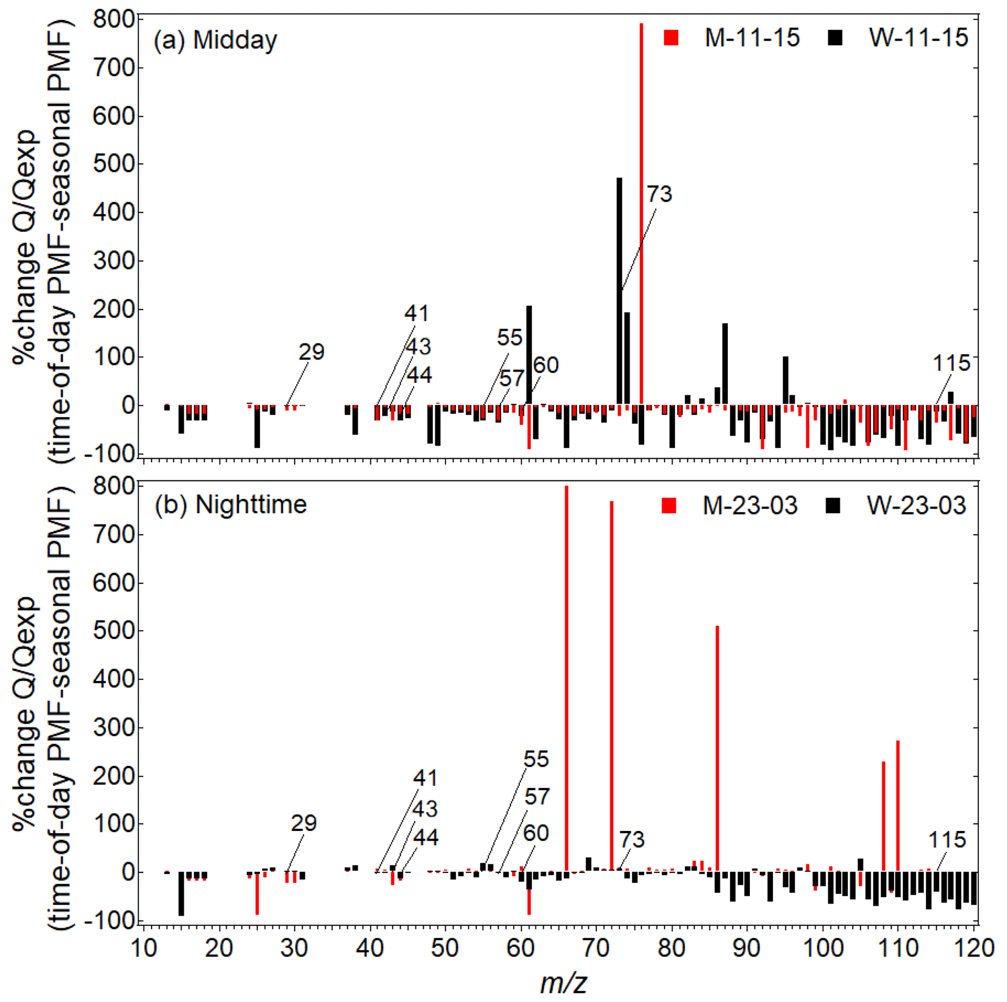
Figure 10Percent change of at different s between the seasonal PMF approach and the time-of-day PMF approach in (a) midday and (b) nighttime periods. Key s show a lower in the time-of-day PMF approach compared to the seasonal PMF approach.
This study introduces a new approach to conducting source apportionment analysis – conducting positive matrix factorization on long-term datasets with each day separated into six 4 h periods with limited variability in emissions and meteorology. The statistical viability of this new source apportionment approach is demonstrated, and the approach is called time-of-day PMF. We apply the time-of-day PMF approach on two seasons of highly time-resolved speciated nonrefractory submicron aerosol (NR-PM1) organics (Org). This dataset was collected as a part of the Delhi Aerosol Supersite (DAS) study. This study improves upon the seasonal source apportionment previously employed in Delhi. We use the EPA PMF tool to apply constraints, extract a larger number of factors, and quantify errors in PMF solutions.
Time-of-day PMF analysis resolves a greater diversity of factors compared to the traditional seasonal PMF approach. In winter, time-of-day PMF separates a mixed SFC-OA factor and a BBOA factor at midday but separates clean HOA and BBOA factors at night. Resolving by time of day allows for the identification of different types of BBOA; the midday BBOA is associated with chloride, and nighttime BBOA is associated with black carbon. In the monsoon, a mixed COA–HOA factor is obtained at midday, but separate clean HOA and COA factors are obtained at night. Even the mixed COA–HOA factor shows clear markers associated with influence of heated cooking oils, especially seen in Asian cooking. Such markers are not seen in seasonal PMF. PMF analysis also separates two OOA factors in each period, one more local and the other more regional in nature. The two OOA factors show signs of mixing and are therefore not discussed in detail.
In the monsoon, the seasonal PMF approach underestimates POA TS at all times of the day relative to the time-of-day PMF approach. In winter, the seasonal PMF approach underestimates POA TS at midday but overestimates POA TS at night. Several differences also occur at key s in POA MS extracted from the two approaches. Time-of-day PMF midday POA factors are more oxidized than the seasonal PMF POA factors, in line with the high photochemical processing at midday. Differences in nighttime POA MS profiles are small.
OOA TS show strong similarity between the two approaches. However, OOA MS show lower oxidation state in the monsoon at midday and in winter at nighttime and higher oxidation state in the monsoon at nighttime and in winter at midday in time-of-day PMF analysis compared to the seasonal PMF analysis. Presence of semi-volatile oxidized organics in the monsoon at midday and in winter at nighttime could be attributed to semi-volatile biogenic emissions in the monsoon and slow oxidation processes in winter respectively.
values of the PMF solutions are a measure of quality of fit and show a decrease of 5 %–30 % going from seasonal PMF analysis to time-of-day PMF analysis. These improvements in can be mapped out to specific time points and s. In winter, improvements in are particularly larger in specific time periods in the 4 h time windows. In the monsoon, the improvements are, for the most part, independent of time. In winter, improvements in are associated with improvements at key s. Improvements in for all periods are partially driven by improvements in fits at s higher than 80.
Application of PMF on field monitoring datasets is a powerful approach to separate the effects of contributing sources. Typically, such analysis is conducted on datasets lasting from a few weeks to a few months. However, in the last decade, several long-term aerosol mass spectrometry deployments have occurred, and one such deployment is the Delhi Aerosol Supersite study. Long-term measurements are also conducted for regulatory-level air pollution monitoring. In the coming years, source apportionment strategies could become mainstream policy tools, and organic mass spectrometry instrumentation may obtain regulatory-grade status. Given this context, the time-of-day PMF approach combines the benefits of large datasets collected using long-term monitoring with the enhancement of time-resolving capability of source apportionment approaches such as PMF at a lower computational intensity compared to the traditional approaches. Results in this paper demonstrate that the time-of-day PMF approach gives a greater number of factors as well as more representative PMF factors compared to the traditional seasonal PMF approach.
| ACSM | Aerosol chemical speciation monitor |
| BBOA | Biomass burning organic aerosol |
| BC | Black carbon |
| BCBB | Wood burning component of BC |
| BCFF | Fossil fuel component of BC |
| BS | Bootstrapping |
| BS-DISP | Bootstrapping enhanced with displacement |
| CO | Carbon monoxide |
| COA | Cooking organic aerosol |
| DAS | Delhi Aerosol Supersite |
| DISP | dQ-controlled displacement of factor elements |
| HOA | Hydrocarbon-like organic aerosol |
| IIT | Indian Institute of Technology |
| LT | Local time |
| ME-2 | Multilinear Engine |
| MS | Mass spectra |
| NCR | National Capital Region |
| NR-PM1 | Nonrefractory submicron particulate matter |
| NR-PM2.5 | Nonrefractory PM smaller than 2.5 µm |
| in diameter | |
| OOA | Oxygenated organic aerosol |
| Org | Organic |
| PBLH | Planetary boundary layer height |
| PET | PMF evaluation tool |
| PM | Particulate matter |
| PM1 | Submicron particulate matter |
| PM2.5 | Particulate matter smaller than 2.5 µm |
| in diameter | |
| PMF | Positive matrix factorization |
| POA | Primary organic aerosol |
| SD | Standard deviation |
| SFC-OA | Solid-fuel combustion organic aerosol |
| SOA | Secondary organic aerosol |
| SoFi | Source Finder |
| SVOOA | Semi-volatile oxygenated organic aerosol |
| SWR | Shortwave radiative flux |
| T | Temperature |
| TS | Time series |
| UVPM | Ultraviolet-absorbing particulate matter |
| VC | Ventilation coefficient |
Data published in this main paper's figures and tables are available via the Texas Data Repository (https://doi.org/10.18738/T8/VIRK5O, Hildebrandt Ruiz and Bhandari, 2022). Underlying research data are also available by request to Lea Hildebrandt Ruiz (lhr@che.utexas.edu).
The supplement related to this article is available online at: https://doi.org/10.5194/amt-15-6051-2022-supplement.
LHR, JSA, GH, and SB designed the study. SB and ZA carried out the data collection. SB carried out the data processing and analysis. SB, JSA, and LHR assisted with the interpretation of results. All co-authors contributed to writing and reviewing the paper.
The contact author has declared that none of the authors has any competing interests.
Publisher’s note: Copernicus Publications remains neutral with regard to jurisdictional claims in published maps and institutional affiliations.
We are thankful to the Indian Institute of Technology (IIT) Delhi for institutional support. We are grateful to all students and staff members of the Aerosol Research Characterization Laboratory (especially Prashant Soni, Nisar Ali Baig, and Mohammad Yawar) and the Environmental Engineering Laboratory (especially Sanjay Gupta) at IIT Delhi for their constant support. We are thankful to Philip Croteau (Aerodyne Research) for always providing timely technical support for the ACSM and Penttti Paatero, Phil Hopke (University of Rochester), and Dave Sullivan (UT Austin) for insightful conversations about PMF. We would also like to thank Nancy Sanchez (now Chevron; then at Rice University) for discussions at the UT Austin Texas Air Quality Symposium that inspired this work. Lastly, we thank Shahzad Gani (University of Helsinki) for leading the instrument setup for the Delhi Aerosol Supersite study.
This research has been supported by the National Science Foundation (grant no. 1653625) and the Welch Foundation (grant nos. F-1925-20170325 and F-1925-20200401).
This paper was edited by Mingjin Tang and reviewed by three anonymous referees.
Abdullahi, K. L., Delgado-Saborit, J. M., and Harrison, R. M.: Emissions and indoor concentrations of particulate matter and its specific chemical components from cooking: a review, Atmos. Environ., 71, 260–294, https://doi.org/10.1016/j.atmosenv.2013.01.061, 2013.
Allan, J. D., Williams, P. I., Morgan, W. T., Martin, C. L., Flynn, M. J., Lee, J., Nemitz, E., Phillips, G. J., Gallagher, M. W., and Coe, H.: Contributions from transport, solid fuel burning and cooking to primary organic aerosols in two UK cities, Atmos. Chem. Phys., 10, 647–668, https://doi.org/10.5194/acp-10-647-2010, 2010.
Amato, F. and Hopke, P. K.: Source apportionment of the ambient PM2.5 across St. Louis using constrained positive matrix factorization, Atmos. Environ., 46, 329–337, https://doi.org/10.1016/j.atmosenv.2011.09.062, 2012.
Amato, F., Pandolfi, M., Escrig, A., Querol, X., Alastuey, A., Pey, J., Perez, N., and Hopke, P. K.: Quantifying road dust resuspension in urban environment by Multilinear Engine: a comparison with PMF2, Atmos. Environ., 43, 2770–2780, https://doi.org/10.1016/j.atmosenv.2009.02.039, 2009.
Amil, N., Latif, M. T., Khan, M. F., and Mohamad, M.: Seasonal variability of PM2.5 composition and sources in the Klang Valley urban-industrial environment, Atmos. Chem. Phys., 16, 5357–5381, https://doi.org/10.5194/acp-16-5357-2016, 2016.
Angelis, E. D., Carnevale, C., Turrini, E., and Volta, M.: Source apportionment and integrated assessment modelling for air quality planning, Electronics, 9, 1098, https://doi.org/10.3390/electronics9071098, 2020.
Arub, Z., Bhandari, S., Gani, S., Apte, J. S., Hildebrandt Ruiz, L., and Habib, G.: Air mass physiochemical characteristics over New Delhi: impacts on aerosol hygroscopicity and cloud condensation nuclei (CCN) formation, Atmos. Chem. Phys., 20, 6953–6971, https://doi.org/10.5194/acp-20-6953-2020, 2020.
Bahreini, R., Keywood, M. D., Ng, N. L., Varutbangkul, V., Gao, S., Flagan, R. C., Seinfeld, J. H., Worsnop, D. R., and Jimenez, J. L.: Measurements of secondary organic aerosol from oxidation of cycloalkenes, terpenes, and m-xylene using an aerodyne aerosol mass spectrometer, Environ. Sci. Technol., 39, 5674–5688, https://doi.org/10.1021/es048061a, 2005.
Belis, C. A., Karagulian, F., Larsen, B. R., and Hopke, P. K.: Critical review and meta-analysis of ambient particulate matter source apportionment using receptor models in Europe, Atmos. Environ., 69, 94–108, https://doi.org/10.1016/j.atmosenv.2012.11.009, 2013.
Belis, C. A., Larsen, B. R., Amato, F., Haddad, E., Favez, O., Harrison, R. M., Hopke, P. K., Nava, S., Paatero, P., Prévôt, A., Quass, U., and Vecchi, R.: European guide on air pollution source apportionment with receptor models, https://publications.jrc.ec.europa.eu/repository/handle/JRC83309 (last access: 10 March 2022), 2014.
Belis, C. A., Karagulian, F., Amato, F., Almeida, M., Artaxo, P., Beddows, D. C., Bernardoni, V., Bove, M. C., Carbone, S., Cesari, D., Contini, D., Cuccia, E., Diapouli, E., Eleftheriadis, K., Favez, O., Haddad, I. E., Harrison, R. M., Hellebust, S., Hovorka, J., Jang, E., Jorquera, H., Kammermeier, T., Karl, M., Lucarelli, F., Mooibroek, D., Nava, S., Nøjgaard, J. K., Paatero, P., Pandolfi, M., Perrone, M. G., Petit, J. E., Pietrodangelo, A., Pokorná, P., Prati, P., Prevot, A. S., Quass, U., Querol, X., Saraga, D., Sciare, J., Sfetsos, A., Valli, G., Vecchi, R., Vestenius, M., Yubero, E., and Hopke, P. K.: A new methodology to assess the performance and uncertainty of source apportionment models II: the results of two European intercomparison exercises, Atmos. Environ., 123, 240–250, https://doi.org/10.1016/j.atmosenv.2015.10.068, 2015.
Bertrand, A., Stefenelli, G., Bruns, E. A., Pieber, S. M., Temime-Roussel, B., Slowik, J. G., Prévôt, A. S., Wortham, H., Haddad, I. E., and Marchand, N.: Primary emissions and secondary aerosol production potential from woodstoves for residential heating: influence of the stove technology and combustion efficiency, Atmos. Environ., 169, 65–79, https://doi.org/10.1016/j.atmosenv.2017.09.005, 2017.
Bhandari, S., Gani, S., Patel, K., Wang, D. S., Soni, P., Arub, Z., Habib, G., Apte, J. S., and Hildebrandt Ruiz, L.: Sources and atmospheric dynamics of organic aerosol in New Delhi, India: insights from receptor modeling, Atmos. Chem. Phys., 20, 735–752, https://doi.org/10.5194/acp-20-735-2020, 2020.
Bhandari, S., Arub, Z., Habib, G., Apte, J. S., and Hildebrandt Ruiz, L.: Contributions of primary sources to submicron organic aerosols in Delhi, India, Atmos. Chem. Phys., 22, 13631–13657, https://doi.org/10.5194/acp-22-13631-2022, 2022.
Bikkina, S., Andersson, A., Kirillova, E. N., Holmstrand, H., Tiwari, S., Srivastava, A. K., Bisht, D. S., and Örjan Gustafsson: Air quality in megacity Delhi affected by countryside biomass burning, Nat. Sustain., 2, 200–205, https://doi.org/10.1038/s41893-019-0219-0, 2019.
Brown, S. G., Lee, T., Norris, G. A., Roberts, P. T., Collett Jr., J. L., Paatero, P., and Worsnop, D. R.: Receptor modeling of near-roadway aerosol mass spectrometer data in Las Vegas, Nevada, with EPA PMF, Atmos. Chem. Phys., 12, 309–325, https://doi.org/10.5194/acp-12-309-2012, 2012.
Brown, S. G., Eberly, S., Paatero, P., and Norris, G. A.: Methods for estimating uncertainty in PMF solutions: examples with ambient air and water quality data and guidance on reporting PMF results, Sci. Total Environm., 518–519, 626–635, https://doi.org/10.1016/j.scitotenv.2015.01.022, 2015.
California Air Resources Board: AB 617 recommended source attribution technical approaches, https://ww2.arb.ca.gov/resources/documents/ab-617-recommended-source-attribution-technical-approaches (last access: 10 March 2022), 2018.
Canonaco, F., Crippa, M., Slowik, J. G., Baltensperger, U., and Prévôt, A. S. H.: SoFi, an IGOR-based interface for the efficient use of the generalized multilinear engine (ME-2) for the source apportionment: ME-2 application to aerosol mass spectrometer data, Atmos. Meas. Tech., 6, 3649–3661, https://doi.org/10.5194/amt-6-3649-2013, 2013.
Canonaco, F., Slowik, J. G., Baltensperger, U., and Prévôt, A. S. H.: Seasonal differences in oxygenated organic aerosol composition: implications for emissions sources and factor analysis, Atmos. Chem. Phys., 15, 6993–7002, https://doi.org/10.5194/acp-15-6993-2015, 2015.
Canonaco, F., Tobler, A., Chen, G., Sosedova, Y., Slowik, J. G., Bozzetti, C., Daellenbach, K. R., El Haddad, I., Crippa, M., Huang, R.-J., Furger, M., Baltensperger, U., and Prévôt, A. S. H.: A new method for long-term source apportionment with time-dependent factor profiles and uncertainty assessment using SoFi Pro: application to 1 year of organic aerosol data, Atmos. Meas. Tech., 14, 923–943, https://doi.org/10.5194/amt-14-923-2021, 2021.
Carslaw, D. C. and Ropkins, K.: openair: an R package for air quality data analysis, Environ. Modell. Softw., 27–28, 52–61, https://doi.org/10.1016/j.envsoft.2011.09.008, 2012.
Chakraborty, J. and Basu, P.: Air Quality and Environmental Injustice in India: Connecting Particulate Pollution to Social Disadvantages, Int. J. Environ. Res. Pub. Health, 18, 304, https://doi.org/10.3390/ijerph18010304, 2021.
Crippa, M., DeCarlo, P. F., Slowik, J. G., Mohr, C., Heringa, M. F., Chirico, R., Poulain, L., Freutel, F., Sciare, J., Cozic, J., Di Marco, C. F., Elsasser, M., Nicolas, J. B., Marchand, N., Abidi, E., Wiedensohler, A., Drewnick, F., Schneider, J., Borrmann, S., Nemitz, E., Zimmermann, R., Jaffrezo, J.-L., Prévôt, A. S. H., and Baltensperger, U.: Wintertime aerosol chemical composition and source apportionment of the organic fraction in the metropolitan area of Paris, Atmos. Chem. Phys., 13, 961–981, https://doi.org/10.5194/acp-13-961-2013, 2013.
Crippa, M., Canonaco, F., Lanz, V. A., Äijälä, M., Allan, J. D., Carbone, S., Capes, G., Ceburnis, D., Dall'Osto, M., Day, D. A., DeCarlo, P. F., Ehn, M., Eriksson, A., Freney, E., Hildebrandt Ruiz, L., Hillamo, R., Jimenez, J. L., Junninen, H., Kiendler-Scharr, A., Kortelainen, A.-M., Kulmala, M., Laaksonen, A., Mensah, A. A., Mohr, C., Nemitz, E., O'Dowd, C., Ovadnevaite, J., Pandis, S. N., Petäjä, T., Poulain, L., Saarikoski, S., Sellegri, K., Swietlicki, E., Tiitta, P., Worsnop, D. R., Baltensperger, U., and Prévôt, A. S. H.: Organic aerosol components derived from 25 AMS data sets across Europe using a consistent ME-2 based source apportionment approach, Atmos. Chem. Phys., 14, 6159–6176, https://doi.org/10.5194/acp-14-6159-2014, 2014.
Crippa, M., Solazzo, E., Huang, G., Guizzardi, D., Koffi, E., Muntean, M., Schieberle, C., Friedrich, R., and Janssens-Maenhout, G.: High resolution temporal profiles in the Emissions Database for Global Atmospheric Research, Sci. Data, 7, 1–17, 2020.
Daellenbach, K. R., Uzu, G., Jiang, J., Cassagnes, L. E., Leni, Z., Vlachou, A., Stefenelli, G. Canonaco, F., Weber, S., Segers, A., Kuenen, J. J., Schaap, M., Favez, O., Albinet, A., Aksoyoglu, S., Dommen, J., Baltensperger, U., Geiser, M., Haddad, I. E., Jaffrezo, J. L., and Prévôt, A. S.: Sources of particulate-matter air pollution and its oxidative potential in Europe, Nature, 587, 414–419, https://doi.org/10.1038/s41586-020-2902-8, 2020.
Dai, Q., Liu, B., Bi, X., Wu, J., Liang, D., Zhang, Y., Feng, Y., and Hopke, P. K.: Dispersion normalized PMF provides insights into the significant changes in source contributions to PM2.5 after the CoviD-19 outbreak, Environ. Sci. Technol., 54, 9917–9927, https://doi.org/10.1021/acs.est.0c02776, 2020.
Dallmann, T. R., Onasch, T. B., Kirchstetter, T. W., Worton, D. R., Fortner, E. C., Herndon, S. C., Wood, E. C., Franklin, J. P., Worsnop, D. R., Goldstein, A. H., and Harley, R. A.: Characterization of particulate matter emissions from on-road gasoline and diesel vehicles using a soot particle aerosol mass spectrometer, Atmos. Chem. Phys., 14, 7585–7599, https://doi.org/10.5194/acp-14-7585-2014, 2014.
Dall'Osto, M., Paglione, M., Decesari, S., Facchini, M. C., O'Dowd, C., Plass-Duellmer, C., and Harrison, R. M.: On the origin of AMS “cooking organic aerosol” at a rural site, Environ. Sci. Technol., 49, 13964–13972, https://pubs.acs.org/doi/abs/10.1021/acs.est.5b02922, 2015.
Drinovec, L., Močnik, G., Zotter, P., Prévôt, A. S. H., Ruckstuhl, C., Coz, E., Rupakheti, M., Sciare, J., Müller, T., Wiedensohler, A., and Hansen, A. D. A.: The ”dual-spot” Aethalometer: an improved measurement of aerosol black carbon with real-time loading compensation, Atmos. Meas. Tech., 8, 1965–1979, https://doi.org/10.5194/amt-8-1965-2015, 2015.
Drosatou, A. D., Skyllakou, K., Theodoritsi, G. N., and Pandis, S. N.: Positive matrix factorization of organic aerosol: insights from a chemical transport model, Atmos. Chem. Phys., 19, 973–986, https://doi.org/10.5194/acp-19-973-2019, 2019.
Environmental Protection Agency: 40 CFR Part 51 Revisions to the guideline on air quality models: enhancements to the AERMOD dispersion modeling system and incorporation of approaches to address ozone and fine particulate matter, https://www.federalregister.gov/documents/2017/01/ (last access: 10 March 2022), 2017.
Fourtziou, L., Liakakou, E., Stavroulas, I., Theodosi, C., Zarmpas, P., Psiloglou, B., Sciare, J., Maggos, T., Bairachtari, K., Bougiatioti, A., Gerasopoulos, E., Sarda-Estève, R., Bonnaire, N., and Mihalopoulos, N.: Multi-tracer approach to characterize domestic wood burning in Athens (Greece) during wintertime, Atmos. Environ., 148, 89–101, https://doi.org/10.1016/j.atmosenv.2016.10.011, 2017.
Fröhlich, R., Crenn, V., Setyan, A., Belis, C. A., Canonaco, F., Favez, O., Riffault, V., Slowik, J. G., Aas, W., Aijälä, M., Alastuey, A., Artiñano, B., Bonnaire, N., Bozzetti, C., Bressi, M., Carbone, C., Coz, E., Croteau, P. L., Cubison, M. J., Esser-Gietl, J. K., Green, D. C., Gros, V., Heikkinen, L., Herrmann, H., Jayne, J. T., Lunder, C. R., Minguillón, M. C., Močnik, G., O'Dowd, C. D., Ovadnevaite, J., Petralia, E., Poulain, L., Priestman, M., Ripoll, A., Sarda-Estève, R., Wiedensohler, A., Baltensperger, U., Sciare, J., and Prévôt, A. S. H.: ACTRIS ACSM intercomparison – Part 2: Intercomparison of ME-2 organic source apportionment results from 15 individual, co-located aerosol mass spectrometers, Atmos. Meas. Tech., 8, 2555–2576, https://doi.org/10.5194/amt-8-2555-2015, 2015.
Gani, S., Bhandari, S., Seraj, S., Wang, D. S., Patel, K., Soni, P., Arub, Z., Habib, G., Hildebrandt Ruiz, L., and Apte, J. S.: Submicron aerosol composition in the world's most polluted megacity: the Delhi Aerosol Supersite study, Atmos. Chem. Phys., 19, 6843–6859, https://doi.org/10.5194/acp-19-6843-2019, 2019.
Gani, S., Bhandari, S., Patel, K., Seraj, S., Soni, P., Arub, Z., Habib, G., Hildebrandt Ruiz, L., and Apte, J. S.: Particle number concentrations and size distribution in a polluted megacity: the Delhi Aerosol Supersite study, Atmos. Chem. Phys., 20, 8533–8549, https://doi.org/10.5194/acp-20-8533-2020, 2020.
Goodkind, A. L., Tessum, C. W., Coggins, J. S., Hill, J. D., and Marshall, J. D.: Fine-scale damage estimates of particulate matter air pollution reveal opportunities for location-specific mitigation of emissions, P. Natl. Acad. Sci. USA, 116, 8775–8780, 2019.
Grolemund, G. and Wickham, H.: Dates and times made easy with lubridate, J. Stat. Softw., 40, 1–25, 2011.
Gunantara, N. and Ai, Q.: A review of multi-objective optimization: methods and its applications, Cog. Eng., 5, 1502242, https://doi.org/10.1080/23311916.2018.1502242, 2018.
Guttikunda, S. K. and Calori, G.: A GIS based emissions inventory at 1 km × 1 km spatial resolution for air pollution analysis in Delhi, India, Atmos. Environ., 67, 101–111, https://doi.org/10.1016/j.atmosenv.2012.10.040, 2013.
Hajat, A., Hsia, C., and O'Neill, M. S.: Socioeconomic disparities and air pollution exposure: a global review, Current Environ. health Rep., 2, 440–450, https://doi.org/10.1007/s40572-015-0069-5, 2015.
Hayfield, T. and Racine, J. S.: Nonparametric econometrics: The np package, J. Stat. Softw., 27, 1–32, https://doi.org/10.18637/jss.v027.i05, 2008.
He, L.-Y., Lin, Y., Huang, X.-F., Guo, S., Xue, L., Su, Q., Hu, M., Luan, S.-J., and Zhang, Y.-H.: Characterization of high-resolution aerosol mass spectra of primary organic aerosol emissions from Chinese cooking and biomass burning, Atmos. Chem. Phys., 10, 11535–11543, https://doi.org/10.5194/acp-10-11535-2010, 2010.
Health Effects Institute: State of global air 2020: special report, https://www.stateofglobalair.org/ (last access: 10 March 2022), 2020.
Heikkinen, L., Äijälä, M., Riva, M., Luoma, K., Dällenbach, K., Aalto, J., Aalto, P., Aliaga, D., Aurela, M., Keskinen, H., Makkonen, U., Rantala, P., Kulmala, M., Petäjä, T., Worsnop, D., and Ehn, M.: Long-term sub-micrometer aerosol chemical composition in the boreal forest: inter- and intra-annual variability, Atmos. Chem. Phys., 20, 3151–3180, https://doi.org/10.5194/acp-20-3151-2020, 2020.
Hemann, J. G., Brinkman, G. L., Dutton, S. J., Hannigan, M. P., Milford, J. B., and Miller, S. L.: Assessing positive matrix factorization model fit: a new method to estimate uncertainty and bias in factor contributions at the measurement time scale, Atmos. Chem. Phys., 9, 497–513, https://doi.org/10.5194/acp-9-497-2009, 2009.
Hildebrandt Ruiz, L. and Bhandari, S.: Data published in “Source apportionment resolved by time of day for improved deconvolution of primary source contributions to air pollution”, Texas Data Repository [data set], https://doi.org/10.18738/T8/VIRK5O, 2022.
Hopke, P. K.: Review of receptor modeling methods for source apportionment, J. Air Waste Manage. Assoc., 66, 237–259, https://doi.org/10.1080/10962247.2016.1140693, 2016.
Hu, W., Hu, M., Hu, W., Jimenez, J. L., Yuan, B., Chen, W., Wang, M., Wu, Y., Chen, C., Wang, Z., Peng, J., Zeng, L., and Shao, M.: Chemical composition, sources, and aging process of submicron aerosols in Beijing: contrast between summer and winter, J. Geophys. Res., 121, 1955–1977, https://doi.org/10.1002/2015JD024020, 2016.
Huang, X.-F., He, L.-Y., Hu, M., Canagaratna, M. R., Sun, Y., Zhang, Q., Zhu, T., Xue, L., Zeng, L.-W., Liu, X.-G., Zhang, Y.-H., Jayne, J. T., Ng, N. L., and Worsnop, D. R.: Highly time-resolved chemical characterization of atmospheric submicron particles during 2008 Beijing Olympic Games using an Aerodyne High-Resolution Aerosol Mass Spectrometer, Atmos. Chem. Phys., 10, 8933–8945, https://doi.org/10.5194/acp-10-8933-2010, 2010.
Indian National Science Academy: Seasons of Delhi, https://www.insaindia.res.in/climate.php (last access: 10 March 2022), 2018.
Intergovernmental Panel on Climate Change, 2019: Summary for Policymakers, in: Climate Change and Land: an IPCC special report on climate change, desertification, land degradation, sustainable land management, food security, and greenhouse gas fluxes in terrestrial ecosystems, https://www.ipcc.ch/srccl/chapter/summary-for-policymakers/ (last access: 10 March 2022), 2019.
Intergovernmental Panel on Climate Change, 2021: Summary for Policymakers, in: Climate Change 2021: The Physical Science Basis. Contribution of Working Group I to the Sixth Assessment Report of the Intergovernmental Panel on Climate Change, https://www.ipcc.ch/report/ar6/wg1/downloads/report/IPCC_AR6_WGI_SPM_final.pdf (last access: 10 March 2022), 2021.
Jimenez, J. L., Canagaratna, M. R., Donahue, N. M., Prevot, A. S., Zhang, Q., Kroll, J. H., DeCarlo, P. F., Allan, J. D., Coe, H., Ng, N. L., Aiken, A. C., Docherty, K. S., Ulbrich, I. M., Grieshop, A. P., Robinson, A. L., Duplissy, J., Smith, J. D., Wilson, K. R., Lanz, V. A., Hueglin, C., Sun, Y. L., Tian, J., Laaksonen, A., Raatikainen, T., Rautiainen, J., Vaattovaara, P., Ehn, M., Kulmala, M., Tomlinson, J. M., Collins, D. R., Cubison, M. J., Dunlea, E. J., Huffman, J. A., Onasch, T. B., Alfarra, M. R., Williams, P. I., Bower, K., Kondo, Y., Schneider, J., Drewnick, F., Borrmann, S., Weimer, S., Demerjian, K., Salcedo, D., Cottrell, L., Griffin, R., Takami, A., Miyoshi, T., Hatakeyama, S., Shimono, A., Sun, J. Y., Zhang, Y. M., Dzepina, K., Kimmel, J. R., Sueper, D., Jayne, J. T., Herndon, S. C., Trimborn, A. M., Williams, L. R., Wood, E. C., Middlebrook, A. M., Kolb, C. E., Baltensperger, U., and Worsnop, D. R.: Evolution of organic aerosols in the atmosphere, Science, 326, 1525–1529, https://science.sciencemag.org/content/326/5959/1525, 2009.
Khare, P., Machesky, J., Soto, R., He, M., Presto, A. A., and Gentner, D. R.: Asphalt-related emissions are a major missing nontraditional source of secondary organic aerosol precursors, Sci. Adv., 6, eabb9785, https://doi.org/10.1126/sciadv.abb9785, 2020.
Kumar, S., Aggarwal, S. G., Gupta, P. K., and Kawamura, K.: Investigation of the tracers for plastic-enriched waste burning aerosols, Atmos. Environ., 108, 49–58, https://doi.org/10.1016/j.atmosenv.2015.02.066, 2015.
Lei, R., Feng, S., and Lauvaux, T.: Country-scale trends in air pollution and fossil fuel CO2 emissions during 2001–2018: confronting the roles of national policies and economic growth, Environ. Res. Lett., 16, 014006, https://doi.org/10.1088/1748-9326/abc9e1, 2021.
Lelieveld, J. and Crutzen, P. J.: The role of clouds in tropospheric photochemistry, J. Atmos. Chem., 12, 229–267, https://link.springer.com/article/10.1007/BF00048075, 1991.
Li, J., Song, Y., Mao, Y., Mao, Z., Wu, Y., Li, M., Huang, X., He, Q., and Hu, M.: Chemical characteristics and source apportionment of PM2.5 during the harvest season in eastern China's agricultural regions, Atmos. Environ., 92, 442–448, https://doi.org/10.1016/j.atmosenv.2014.04.058, 2014a.
Li, J., Wang, G., Aggarwal, S. G., Huang, Y., Ren, Y., Zhou, B., Singh, K., Gupta, P. K., Cao, J., and Zhang, R.: Comparison of abundances, compositions and sources of elements, inorganic ions and organic compounds in atmospheric aerosols from Xi'an and New Delhi, two megacities in China and India, Sci. Total Environ., 476–477, 485–495, https://doi.org/10.1016/j.scitotenv.2014.01.011, 2014b.
Lin, C., Ceburnis, D., Hellebust, S., Buckley, P., Wenger, J., Canonaco, F., Prévôt, A. S. H., Huang, R. J., O'Dowd, C., and Ovadnevaite, J.: Characterization of primary organic aerosol from domestic wood, peat, and coal burning in Ireland, Environ. Sci. Technol., 51, 10624–10632, https://doi.org/10.1021/acs.est.7b01926, 2017.
Liu, Q., Sun, Y., Hu, B., Liu, Z. R., Akio, S., and Wang, Y. S.: In situ measurement of PM1 organic aerosol in Beijing winter using a high-resolution aerosol mass spectrometer, Chinese Sci. Bull., 57, 819–826, https://doi.org/10.1007/s11434-011-4886-0, 2012.
Liu, T., Wang, Z., Wang, X., and Chan, C. K.: Primary and secondary organic aerosol from heated cooking oil emissions, Atmos. Chem. Phys., 18, 11363–11374, https://doi.org/10.5194/acp-18-11363-2018, 2018.
Lu, J. G.: Air pollution: a systematic review of its psychological, economic, and social effects, Curr. Opinion Psychol., 32, 52–65, https://doi.org/10.1016/j.copsyc.2019.06.024, 2020.
Mishra, R. K., Pandey, A., Pandey, G., and Kumar, A.: The effect of odd-even driving scheme on PM2.5 and PM1.0 emission, Transport. Res. Part D: Transport and Environment, 67, 541–552, https://doi.org/10.1016/j.trd.2019.01.005, 2019.
Misra, P., Imasu, R., Hayashida, S., Arbain, A. A., Avtar, R., and Takeuchi, W.: Mapping brick kilns to support environmental impact studies around Delhi using Sentinel-2, ISPRS Int. J. Geo-Inform., 9, 544, https://doi.org/10.3390/ijgi9090544, 2020.
Ng, N. L., Canagaratna, M. R., Zhang, Q., Jimenez, J. L., Tian, J., Ulbrich, I. M., Kroll, J. H., Docherty, K. S., Chhabra, P. S., Bahreini, R., Murphy, S. M., Seinfeld, J. H., Hildebrandt, L., Donahue, N. M., DeCarlo, P. F., Lanz, V. A., Prévôt, A. S. H., Dinar, E., Rudich, Y., and Worsnop, D. R.: Organic aerosol components observed in Northern Hemispheric datasets from Aerosol Mass Spectrometry, Atmos. Chem. Phys., 10, 4625–4641, https://doi.org/10.5194/acp-10-4625-2010, 2010.
Ng, N. L., Canagaratna, M. R., Jimenez, J. L., Zhang, Q., Ulbrich, I. M., and Worsnop, D. R.: Realtime methods for estimating organic component mass concentrations from aerosol mass spectrometer data, Environ. Sci. Technol., 45, 910–916, https://doi.org/10.1021/es102951k, 2011a.
Ng, N. L., Herndon, S. C., Trimborn, A., Canagaratna, M. R., Croteau, P. L., Onasch, T. B., Sueper, D., Worsnop, D. R., Zhang, Q., Sun, Y. L., and Jayne, J. T.: An Aerosol Chemical Speciation Monitor (ACSM) for routine monitoring of the composition and mass concentrations of ambient aerosol, Aerosol Scie. Technol., 45, 780–794, https://doi.org/10.1080/02786826.2011.560211, 2011b.
Norris, G., Duvall, R., Brown, S., and Bai, S.: EPA Positive Matrix Factorization 5.0 fundamentals and user guide, https://www.epa.gov/air-research/epa-positive-matrix-factorization-50-fundamentals-and-user-guide (last access: 10 March 2022), 2014.
Olson, M. R., Garcia, M. V., Robinson, M. A., Rooy, P. V., Dietenberger, M. A., Bergin, M., and Schauer, J. J.: Investigation of black and brown carbon multiple-wavelength dependent light absorption from biomass and fossil fuel combustion source emissions, J. Geophys. Res., 120, 6682–6697, https://doi.org/10.1002/2014JD022970, 2015.
Organization for Economic Co-operation and Development: The economic cost of air pollution: evidence from Europe, https://www.oecd-ilibrary.org/economics/the-economic-cost-of-air-pollution-evidence-from-europe_56119490-en (last access: 10 March 2022), 2020.
Paatero, P.: Least squares formulation of robust non-negative factor analysis, Chemomet. Intell. Labor. Syst., 37, 23–35, https://doi.org/10.1016/S0169-7439(96)00044-5, 1997.
Paatero, P.: The Multilinear Engine – a table-driven, least squares program for solving multilinear problems, including the n-way parallel factor analysis model, J. Comput. Graph. Stat., 8, 854–888, https://doi.org/10.1080/10618600.1999.10474853, 1999.
Paatero, P. and Hopke, P. K.: Discarding or downweighting high-noise variables in factor analytic models, Anal. Chim. Acta, 490, 277–289, https://doi.org/10.1016/S0003-2670(02)01643-4, 2003.
Paatero, P. and Hopke, P. K.: Rotational tools for factor analytic models, J. Chemomet., 23, 91–100, https://doi.org/10.1002/cem.1197, 2009.
Paatero, P. and Tapper, U.: Positive matrix factorization: a non-negative factor model with optimal utilization of error estimates of data values, Environmetrics, 5, 111–126, https://doi.org/10.1002/env.3170050203, 1994.
Paatero, P., Hopke, P. K., Song, X. H., and Ramadan, Z.: Understanding and controlling rotations in factor analytic models, Chemomet. Intell. Labor. Syst., 60, 253–264, https://doi.org/10.1016/S0169-7439(01)00200-3, 2002.
Paatero, P., Eberly, S., Brown, S. G., and Norris, G. A.: Methods for estimating uncertainty in factor analytic solutions, Atmos. Meas. Tech., 7, 781–797, https://doi.org/10.5194/amt-7-781-2014, 2014.
Pandey, A., Brauer, M., Cropper, M. L., Balakrishnan, K., Mathur, P., Dey, S., Turkgulu, B., Kumar, G. A., Khare, M., Beig, G., Gupta, T., Krishnankutty, R. P., Causey, K., Cohen, A. J., Bhargava, S., Aggarwal, A. N., Agrawal, A., Awasthi, S., Bennitt, F., Bhagwat, S., Bhanumati, P., Burkart, K., Chakma, J. K., Chiles, T. C., Chowdhury, S., Christopher, D. J., Dey, S., Fisher, S., Fraumeni, B., Fuller, R., Ghoshal, A. G., Golechha, M. J., Gupta, P. C., Gupta, R., Gupta, R., Gupta, S., Guttikunda, S., Hanrahan, D., Harikrishnan, S., Jeemon, P., Joshi, T. K., Kant, R., Kant, S., Kaur, T., Koul, P. A., Kumar, P., Kumar, R., Larson, S. L., Lodha, R., Madhipatla, K. K., Mahesh, P. A., Malhotra, R., Managi, S., Martin, K., Mathai, M., Mathew, J. L., Mehrotra, R., Mohan, B. V. M., Mohan, V., Mukhopadhyay, S., Mutreja, P., Naik, N., Nair, S., Pandian, J. D., Pant, P., Perianayagam, A., Prabhakaran, D., Prabhakaran, P., Rath, G. K., Ravi, S., Roy, A., Sabde, Y. D., Salvi, S., Sambandam, S., Sharma, B., Sharma, M., Sharma, S., Sharma, R. S., Shrivastava, A., Singh, S., Singh, V., Smith, R., Stanaway, J. D., Taghian, G., Tandon, N., Thakur, J. S., Thomas, N. J., Toteja, G. S., Varghese, C. M., Venkataraman, C., Venugopal, K. N., Walker, K. D., Watson, A. Y., Wozniak, S., Xavier, D., Yadama, G. N., Yadav, G., Shukla, D. K., Bekedam, H. J., Reddy, K. S., Guleria, R., Vos, T., Lim, S. S., Dandona, R., Kumar, S., Kumar, P., Landrigan, P. J., and Dandona, L.: Health and economic impact of air pollution in the states of India: the Global Burden of Disease Study 2019, The Lancet Planet. Health, 5, 25–38, https://doi.org/10.1016/S2542-5196(20)30298-9, 2020.
Park, M. B., Lee, T. J., Lee, E. S., and Kim, D. S.: Enhancing source identification of hourly PM2.5 data in Seoul based on a dataset segmentation scheme by positive matrix factorization (PMF), Atmos. Pollut. Res., 10, 1042–1059, https://doi.org/10.1016/j.apr.2019.01.013, 2019.
Patel, K., Bhandari, S., Gani, S., Campmier, M. J., Kumar, P., Habib, G., Apte, J., and Ruiz, L. H.: Sources and dynamics of submicron aerosol during the Autumn onset of the air pollution season in Delhi, India, ACS Earth and Space Chemistry, https://doi.org/10.1021/acsearthspacechem.0c00340, 2021a.
Patel, K., Campmier, M. J., Bhandari, S., Baig, N., Gani, S., Habib, G., Apte, J. S., and Hildebrandt Ruiz, L.: Persistence of Primary and Secondary Pollutants in Delhi: Concentrations and Composition from 2017 through the COVID Pandemic, Environ. Sci. Technol. Lett., 8, 492–497, https://doi.org/10.1021/acs.estlett.1c00211, 2021b.
Patel, S., Sankhyan, S., Boedicker, E. K., Decarlo, P. F., Farmer, D. K., Goldstein, A. H., Katz, E. F., Nazaroff, W. W., Tian, Y., Vanhanen, J., and Vance, M. E.: Indoor particulate matter during HOMEChem: concentrations, size distributions, and exposures, Environ. Sci. Technol., 54, 7107–7116, https://doi.org/10.1021/acs.est.0c00740, 2020.
Patton, A., Politis, D. N., and White, H.: Correction to automatic block-length selection for the dependent bootstrap by D. Politis and H. White, Econom. Rev., 28, 372–375, https://doi.org/10.1080/07474930802459016, 2009.
Pauraite, J., Pivoras, A., Plauškaite, K., Bycenkiene, S., Mordas, G., Augustaitis, A., Marozas, V., Mozgeris, G., Baumgarten, M., Matyssek, R., and Ulevicius, V.: Characterization of aerosol mass spectra responses to temperature over a forest site in Lithuania, J. Aerosol Sci., 133, 56–65, https://doi.org/10.1016/j.jaerosci.2019.03.010, 2019.
Politis, D. N. and White, H.: Automatic block-length selection for the dependent bootstrap, Econom. Rev., 23, 53–70, https://doi.org/10.1081/ETC-120028836, 2004.
Rai, P., Furger, M., Slowik, J. G., Canonaco, F., Fröhlich, R., Hüglin, C., Minguillón, M. C., Petterson, K., Baltensperger, U., and Prévôt, A. S. H.: Source apportionment of highly time-resolved elements during a firework episode from a rural freeway site in Switzerland, Atmos. Chem. Phys., 20, 1657–1674, https://doi.org/10.5194/acp-20-1657-2020, 2020.
R Core Team: R: a language and environment for statistical computing, R Foundation for Statistical Computing, Vienna, Austria, https://www.R-project.org/ (last access: 10 March 2022), 2019.
Ramadan, Z., Eickhout, B., Song, X. H., Buydens, L. M., and Hopke, P. K.: Comparison of Positive Matrix Factorization and Multilinear Engine for the source apportionment of particulate pollutants, Chemomet. Intellig. Labor. Syst., 66, 15–28, https://doi.org/10.1016/S0169-7439(02)00160-0, 2003.
Reyes-Villegas, E., Green, D. C., Priestman, M., Canonaco, F., Coe, H., Prévôt, A. S. H., and Allan, J. D.: Organic aerosol source apportionment in London 2013 with ME-2: exploring the solution space with annual and seasonal analysis, Atmos. Chem. Phys., 16, 15545–15559, https://doi.org/10.5194/acp-16-15545-2016, 2016.
Reyes-Villegas, E., Priestley, M., Ting, Y.-C., Haslett, S., Bannan, T., Le Breton, M., Williams, P. I., Bacak, A., Flynn, M. J., Coe, H., Percival, C., and Allan, J. D.: Simultaneous aerosol mass spectrometry and chemical ionisation mass spectrometry measurements during a biomass burning event in the UK: insights into nitrate chemistry, Atmos. Chem. Phys., 18, 4093–4111, https://doi.org/10.5194/acp-18-4093-2018, 2018.
Robinson, E. S., Gu, P., Ye, Q., Li, H. Z., Shah, R. U., Apte, J. S., Robinson, A. L., and Presto, A. A.: Restaurant impacts on outdoor air quality: elevated organic aerosol mass from restaurant cooking with neighborhood-scale plume extents, Environ. Sci. Technol., 52, 9285–9294, https://pubs.acs.org/doi/abs/10.1021/acs.est.8b02654, 2018.
Sandradewi, J., Prévôt, A. S., Szidat, S., Perron, N., Alfarra, M. R., Lanz, V. A., Weingartner, E., and Baltensperger, U. R.: Using aerosol light abosrption measurements for the quantitative determination of wood burning and traffic emission contribution to particulate matter, Environ. Sci. Technol., 42, 3316–3323, https://doi.org/10.1021/es702253m, 2008.
Schlag, P., Kiendler-Scharr, A., Blom, M. J., Canonaco, F., Henzing, J. S., Moerman, M., Prévôt, A. S. H., and Holzinger, R.: Aerosol source apportionment from 1-year measurements at the CESAR tower in Cabauw, the Netherlands, Atmos. Chem. Phys., 16, 8831–8847, https://doi.org/10.5194/acp-16-8831-2016, 2016.
Schneider, J., Weimer, S., Drewnick, F., Borrmann, S., Helas, G., Gwaze, P., Schmid, O., Andreae, M. O., and Kirchner, U.: Mass spectrometric analysis and aerodynamic properties of various types of combustion-related aerosol particles, Int. J. Mass Spectro., 258, 37–49, https://doi.org/10.1016/j.ijms.2006.07.008, 2006.
Schraufnagel, D. E., Balmes, J. R., Cowl, C. T., Matteis, S. D., Jung, S. H., Mortimer, K., Perez Padilla, R., Rice, M. B., Riojas-Rodriguez, H., Sood, A., Thurston, G. D., To, T., Vanker, A., and Wuebbles, D. J.: Air pollution and noncommunicable diseases: a review by the Forum of International Respiratory Societies' Environmental Committee, part 1: the damaging effects of air pollution, Chest, 155, 409–416, https://doi.org/10.1016/j.chest.2018.10.042, 2019.
Shaddick, G., Thomas, M. L., Mudu, P., Ruggeri, G., and Gumy, S.: Half the world's population are exposed to increasing air pollution, npj Clim. Atmos. Sci., 3, 1–5, https://doi.org/10.1038/s41612-020-0124-2, 2020.
Stavroulas, I., Bougiatioti, A., Grivas, G., Paraskevopoulou, D., Tsagkaraki, M., Zarmpas, P., Liakakou, E., Gerasopoulos, E., and Mihalopoulos, N.: Sources and processes that control the submicron organic aerosol composition in an urban Mediterranean environment (Athens): a high temporal-resolution chemical composition measurement study, Atmos. Chem. Phys., 19, 901–919, https://doi.org/10.5194/acp-19-901-2019, 2019.
Sun, Y.-L., Zhang, Q., Schwab, J. J., Demerjian, K. L., Chen, W.-N., Bae, M.-S., Hung, H.-M., Hogrefe, O., Frank, B., Rattigan, O. V., and Lin, Y.-C.: Characterization of the sources and processes of organic and inorganic aerosols in New York city with a high-resolution time-of-flight aerosol mass apectrometer, Atmos. Chem. Phys., 11, 1581–1602, https://doi.org/10.5194/acp-11-1581-2011, 2011.
Sun, Y. L., Wang, Z. F., Fu, P. Q., Yang, T., Jiang, Q., Dong, H. B., Li, J., and Jia, J. J.: Aerosol composition, sources and processes during wintertime in Beijing, China, Atmos. Chem. Phys., 13, 4577–4592, https://doi.org/10.5194/acp-13-4577-2013, 2013.
Tessum, C. W., Apte, J. S., Goodkind, A. L., Muller, N. Z., Mullins, K. A., Paolella, D. A., Polasky, S., Springer, N. P., Thakrar, S. K., Marshall, J. D., and Hill, J. D.: Inequity in consumption of goods and services adds to racial-ethnic disparities in air pollution exposure, P. Natl. Acad. Sci. USA, 116, 6001–6006, https://doi.org/10.1073/pnas.1818859116, 2019.
Thakrar, S. K., Balasubramanian, S., Adams, P. J., Azevedo, I. M., Muller, N. Z., Pandis, S. N., Polasky, S., Pope, C. A., Robinson, A. L., Apte, J. S., Tessum, C. W., Marshall, J. D., and Hill, J. D.: Reducing mortality from air pollution in the United States by targeting specific emission sources, Environ. Sci. Technol. Lett., 7, 639–645, https://doi.org/10.1021/acs.estlett.0c00424, 2020.
Thamban, N. M., Tripathi, S. N., Moosakutty, S. P., Kuntamukkala, P., and Kanawade, V. P.: Internally mixed black carbon in the Indo-Gangetic Plain and its effect on absorption enhancement, Atmos. Res., 197, 211–223, https://doi.org/10.1016/j.atmosres.2017.07.007, 2017.
Thind, M. P., Tessum, C. W., Azevedo, I. L., and Marshall, J. D.: Fine particulate air pollution from electricity generation in the US: health impacts by race, income, and geography, Environ. Sci. Technol., 53, 14010–14019, https://pubs.acs.org/doi/abs/10.1021/acs.est.9b02527, 2019.
Tian, J., Wang, Q., Ni, H., Wang, M., Zhou, Y., Han, Y., Shen, Z., Pongpiachan, S., Zhang, N., Zhao, Z., Zhang, Q., Zhang, Y., Long, X., and Cao, J.: Emission characteristics of primary brown carbon absorption from biomass and coal burning: development of an optical emission inventory for China, J. Geophys. Res.-Atmos., 124, 1879–1893, https://onlinelibrary.wiley.com/doi/abs/10.1029/2018JD029352, 2019.
Tian, Y., Xiao, Z., Wang, H., Peng, X., Guan, L., Huangfu, Y., Shi, G., Chen, K., Bi, X., and Feng, Y.: Influence of the sampling period and time resolution on the PM source apportionment: study based on the high time-resolution data and long-term daily data, Atmos. Environ., 165, 301–309, https://doi.org/10.1016/j.atmosenv.2017.07.003, 2017.
Tobler, A., Bhattu, D., Canonaco, F., Lalchandani, V., Shukla, A., Thamban, N. M., Mishra, S., Srivastava, A. K., Bisht, D. S., Tiwari, S., Singh, S., Mocnik, G., Baltensperger, U., Tripathi, S. N., Slowik, J. G., and Prévôt, A. S.: Chemical characterization of PM2.5 and source apportionment of organic aerosol in New Delhi, India, Sci. Total Environ., 745, 140924, https://doi.org/10.1016/j.scitotenv.2020.140924, 2020.
Tschofen, P., Azevedo, I. L., and Muller, N. Z.: Fine particulate matter damages and value added in the US economy, P. Natl. Acad. Sci. USA, 116, 19857–19862, https://doi.org/10.1073/pnas.1905030116, 2019.
Ulbrich, I. M., Canagaratna, M. R., Zhang, Q., Worsnop, D. R., and Jimenez, J. L.: Interpretation of organic components from Positive Matrix Factorization of aerosol mass spectrometric data, Atmos. Chem. Phys., 9, 2891–2918, https://doi.org/10.5194/acp-9-2891-2009, 2009.
Ulbrich, I. M., Handschy, A., Lechner, M., and Jimenez, J.: AMS Spectral Database, http://cires.colorado.edu/jimenez-group/AMSsd/ (last access: 25 April 2019), 2017.
Ulbrich, I. M., Handschy, A., Lechner, M., and Jimenez, J.: High-Resolution AMS Spectral Database, http://cires.colorado.edu/jimenez-group/HRAMSsd/ (last access: 25 April 2019), 2018.
Venables, W. N. and Ripley, B. D.: Modern applied statistics with S, Springer, New York, fourth Edn., http://www.stats.ox.ac.uk/pub/MASS4 (last access: 10 March 2022), 2002.
Venturini, E., Vassura, I., Raffo, S., Ferroni, L., Bernardi, E., and Passarini, F.: Source apportionment and location by selective wind sampling and Positive Matrix Factorization, Environ. Sci. Pollut. Res., 21, 11634–11648, https://doi.org/10.1007/s11356-014-2507-6, 2014.
Wang, Q., Qiao, L., Zhou, M., Zhu, S., Griffith, S., Li, L., and Yu, J. Z.: Source apportionment of PM2.5 using hourly measurements of elemental tracers and major constituents in an urban environment: investigation of time-resolution influence, J. Geophys. Res.-Atmos., 123, 5284–5300, https://doi.org/10.1029/2017JD027877, 2018.
Wang, Y., Hopke, P. K., Rattigan, O. V., Xia, X., Chalupa, D. C., and Utell, M. J.: Characterization of residential wood combustion particles using the two-wavelength aethalometer, Environ. Sci. Technol., 45, 7387–7393, https://doi.org/10.1021/es2013984, 2011.
Wayland, R. A.: EPA modeling guidance for demonstrating attainment of air quality goals for ozone, PM2.5, and regional haze, https://www.epa.gov/scram/state-implementation-plan-sip-attainment-demonstration-guidance (last access: 10 March 2022), 2018.
Wickham, H., Averick, M., Bryan, J., Chang, W., McGowan, L. D., François, R., Grolemund, G., Hayes, A., Henry, L., Hester, J., Kuhn, M., Pedersen, T. L., Miller, E., Bache, S. M., Müller, K., Ooms, J., Robinson, D., Seidel, D. P., Spinu, V., Takahashi, K., Vaughan, D., Wilke, C., Woo, K., and Yutani, H.: Welcome to the tidyverse, Journal of Open Source Software, 4, 1686, https://doi.org/10.21105/joss.01686), 2019.
Williams, B. J., Goldstein, A. H., Kreisberg, N. M., Hering, S. V., Worsnop, D. R., Ulbrich, I. M., Docherty, K. S., and Jimenez, J. L.: Major components of atmospheric organic aerosol in southern California as determined by hourly measurements of source marker compounds, Atmos. Chem. Phys., 10, 11577–11603, https://doi.org/10.5194/acp-10-11577-2010, 2010.
World Health Organization: AAP air quality database, http://www.who.int/phe/health_topics/outdoorair/databases/cities/en/ (last access: 20 December 2020), 2018.
Xie, M., Barsanti, K. C., Hannigan, M. P., Dutton, S. J., and Vedal, S.: Positive matrix factorization of PM2.5 – eliminating the effects of gas/particle partitioning of semivolatile organic compounds, Atmos. Chem. Phys., 13, 7381–7393, https://doi.org/10.5194/acp-13-7381-2013, 2013a.
Xie, M., Piedrahita, R., Dutton, S. J., Milford, J. B., Hemann, J. G., Peel, J. L., Miller, S. L., Kim, S. Y., Vedal, S., Sheppard, L., and Hannigan, M. P.: Positive matrix factorization of a 32-month series of daily PM2.5 speciation data with incorporation of temperature stratification, Atmos. Environ., 65, 11–20, https://doi.org/10.1016/j.atmosenv.2012.09.034, 2013b.
Zhang, K. and Batterman, S.: Air pollution and health risks due to vehicle traffic, Sci. Total Environ., 450–451, 307–316, https://doi.org/10.1016/j.scitotenv.2013.01.074, 2013.
Zhang, Q., Alfarra, M. R., Worsnop, D. R., Allan, J. D., Coe, H., Canagaratna, M. R., and Jimenez, J. L.: Deconvolution and quantification of hydrocarbon-like and oxygenated organic aerosols based on aerosol mass spectrometry, Environ. Sci. Technol., 39, 4938–4952, https://pubs.acs.org/doi/abs/10.1021/es048568l, 2005.
Zhang, Q., Jimenez, J. L., Canagaratna, M. R., Ulbrich, I. M., Ng, N. L., Worsnop, D. R., and Sun, Y.: Understanding atmospheric organic aerosols via factor analysis of aerosol mass spectrometry: a review, Analyt. Bioanalyt. Chem., 401, 3045–3067, https://link.springer.com/article/10.1007/s00216-011-5355-y, 2011.
Zhang, Y., Favez, O., Petit, J.-E., Canonaco, F., Truong, F., Bonnaire, N., Crenn, V., Amodeo, T., Prévôt, A. S. H., Sciare, J., Gros, V., and Albinet, A.: Six-year source apportionment of submicron organic aerosols from near-continuous highly time-resolved measurements at SIRTA (Paris area, France), Atmos. Chem. Phys., 19, 14755–14776, https://doi.org/10.5194/acp-19-14755-2019, 2019.
Zhang, Z., Zhu, W., Hu, M., Wang, H., Chen, Z., Shen, R., Yu, Y., Tan, R., and Guo, S.: Secondary organic aerosol from typical Chinese domestic cooking emissions, Environ. Sci. Technol. Lett., 8, 1, https://doi.org/10.1021/acs.estlett.0c00754, 2020.
Zheng, Y., Cheng, X., Liao, K., Li, Y., Li, Y. J., Huang, R.-J., Hu, W., Liu, Y., Zhu, T., Chen, S., Zeng, L., Worsnop, D. R., and Chen, Q.: Characterization of anthropogenic organic aerosols by TOF-ACSM with the new capture vaporizer, Atmos. Meas. Tech., 13, 2457–2472, https://doi.org/10.5194/amt-13-2457-2020, 2020.
Zhu, Q., Huang, X.-F., Cao, L.-M., Wei, L.-T., Zhang, B., He, L.-Y., Elser, M., Canonaco, F., Slowik, J. G., Bozzetti, C., El-Haddad, I., and Prévôt, A. S. H.: Improved source apportionment of organic aerosols in complex urban air pollution using the multilinear engine (ME-2), Atmos. Meas. Tech., 11, 1049–1060, https://doi.org/10.5194/amt-11-1049-2018, 2018.