the Creative Commons Attribution 4.0 License.
the Creative Commons Attribution 4.0 License.
 | 25 Oct 2022
SAGE III/ISS ozone and NO2 validation using diurnal scaling factors
Ghassan Taha
Luke D. Oman
Robert Damadeo
David Flittner
Mark Schoeberl
Christopher E. Sioris
Ryan Stauffer
We developed a set of solar zenith angle, latitude- and altitude-dependent scaling factors to account for the diurnal variability in ozone (O3) and nitrogen dioxide (NO2) when comparing Stratospheric Aerosol and Gas Experiment (SAGE) III/ISS observations to observations from other times of day. The scaling factors are calculated as a function of solar zenith angle from the four-dimensional output of a global atmospheric chemistry model simulation of 2017–2020 that shows good agreement with observed vertical profiles. Using a global atmospheric chemistry model allows us to account for both chemically and dynamically driven variability. Both year-specific scale factors and a multi-year monthly climatology are available to decrease the uncertainty in inter-instrument comparisons and allow consistent comparisons between observations from different times of day. We describe the variability in the diurnal scale factors as a function of space and time. The quasi-biennial oscillation (QBO) appears to be a contributing factor to interannual variability in the NO2 scaling factors, leading to differences between years that switch sign with altitude. We show that application of these scaling factors improves the comparison between SAGE III/ISS and OSIRIS NO2 and between SAGE III/ISS and OMPS LP, OSIRIS, and ACE-FTS O3 observations. The comparisons between SAGE III/ISS O3 for sunrise or sunset vs. Microwave Limb Sounder (MLS) daytime or nighttime observations are also more consistent when we apply the diurnal scaling factors. There is good agreement between SAGE III/ISS V5.2 ozone and correlative measurements, with differences within 5 % between 20 and 50 km when corrected for diurnal variability. Similarly, the SAGE III/ISS V5.2 NO2 agreement with correlative measurement is mostly within 10 %. While the scale factors were designed for use with SAGE III/ISS observations, they can easily be applied to other observation intercomparisons as well.
- Article
(6791 KB) - Full-text XML
-
Supplement
(681 KB) - BibTeX
- EndNote


Observations from the Stratospheric Aerosol and Gas Experiment (SAGE) III began in 2017 following its successful docking with the International Space Station (ISS). SAGE III/ISS measures vertical profiles of ozone (O3), nitrogen dioxide (NO2), and water vapor as well as cloud presence using solar occultation measurements (McCormick et al., 1989; Wang et al., 2006; Schoeberl et al., 2021). Observations are thus available at both sunrise and sunset. It also provides profiles of aerosol extinction at multiple visible, near-infrared, and ultraviolet wavelengths. SAGE III/ISS extends the SAGE series of solar occultation instruments that began with the Stratospheric Aerosol Measurement (SAM) in July 1975 and includes SAM II, which flew from 1978 to 1993, SAGE I, which launched in 1979, SAGE II, launched in 1984, and SAGE III Meteor, launched in 2001. SAGE I/II instruments were heavily used in long-term trend studies because of their precise measurements and long data record (WMO, 1988, 2011; Harris et al., 2015). Accurate, continuous measurements of stratospheric NO2 are necessary because of the important role of NO2 in the Earth's O3 distribution (Crutzen, 1979).
Stratospheric NO2 experiences a strong diurnal cycle. Photolysis of NO2 leads to a rapid drop in concentration at sunrise, while NO2 concentrations rapidly rise at sunset as NO is converted to NO2 (e.g., Brohede et al., 2007; Solomon et al., 1986, and references therein). Previous studies often used the PRATMO (Prather, 1992; Prather and Jaffe, 1990) photochemical box model to account for diurnal variability in NO2 when comparing observations from different times of day (Brohede et al., 2007; Dubé et al., 2020) and to account for NO2 variability along the line of sight (Dubé et al., 2021). Using PRATMO, Dubé et al. (2021) showed a diurnal range exceeding a factor of 3 for NO2 at the Equator at 30 km.
O3 also experiences a diurnal cycle due to photochemistry. This cycle is large in the upper stratosphere and mesosphere (e.g., Vaughan, 1982; Prather, 1981) but also exceeds 2 % in the mid-stratosphere (Sakazaki et al., 2013; Parrish et al., 2014). Frith et al. (2020) found that the O3 diurnal cycle exceeds 15 % in the upper stratosphere near the edge of the polar day. Model simulations suggest diurnal variability in the tropospheric O3 column can reach over 9 DU in some locations and changes over time due to evolving precursor emissions (Strode et al., 2019). Damadeo et al. (2018) found that biases in diurnal sampling in occultation instruments can affect O3 trend calculations due to changes over time in the relative frequency of sunrise and sunset measurements combined with diurnal variability. Accounting for the diurnal cycle above 35 km allows a more direct comparison between SAGE III/ISS observations and observations from instruments that measure at different times of day, such as the Microwave Limb Sounder (MLS) (Waters et al., 2006) on the Aura satellite (Schoeberl et al., 2006), which measures O3 at midday and in the middle of the night outside of the polar regions, where sampling occurs over a wider range of local times. Estimates of the diurnal variability also provide a basis for comparison of the sunrise vs. sunset measurements with SAGE III/ISS (Wang et al., 2020). In order to account for differences in sampling times between ozone instruments, Frith et al. (2020) used a global model simulation to develop a climatology of O3 diurnal variability based on time of day.
In this work, we create diurnal scaling factors for ozone and NO2 as a function of solar zenith angle (SZA), latitude, and altitude for each month and year of the SAGE III/ISS period. We use a global model to account for vertical, horizontal, and temporal differences in NO2 and O3 due to both chemistry and transport. Studer et al. (2014) found interannual variability in the diurnal cycle of stratospheric and mesospheric O3 above Switzerland. We therefore develop year-specific diurnal scale factors as well as climatological diurnal scaling factors. The resulting scale factors are publicly available and provide a convenient resource for accounting for the diurnal cycle when comparing observations from SAGE III/ISS or other instruments to observations from other times of day. This allows a greater number of observations to be directly compared since the observations can occur at different times of day.
We describe the model and methods used to develop diurnal scaling factors in Sect. 2 and evaluate the simulated O3 and NO2 with observations in Sect. 3. Section 4 presents the geographic and temporal variability of the scaling factors and demonstrates their application to measurement comparisons for NO2 and O3. We present conclusions in Sect. 5.
2.1 Instrument descriptions
2.1.1 SAGE III/ISS
The SAGE III/ISS instrument was launched to the ISS on 19 February 2017. The instrument scans over the Sun during sunrise and sunset events, measuring the atmospheric extinction along the line of sight (Cisewski et al., 2014). SAGE III/ISS profiles are produced on a 0.5 km grid with an estimated vertical resolution of 0.7 km from 10 to 50 km for NO2 and from 6 to 85 km for O3 (SAGE III Algorithm Theoretical Basis Document, 2002). SAGE III coverage and number of profiles are limited to about 15 sunrise and 15 sunset events per day, with the majority of observations occurring between 60∘ S and 60∘ N. Dubé et al. (2021) reported that the SAGE III/ISS NO2 V5.1 is over 20 % biased high in much of the mid-stratosphere even when accounting for diurnal variability. We also use the “aerosol ozone” (AO3) ozone retrieval, which is similar to the SAGE II retrieval method (Damadeo et al., 2013), as recommended by Wang et al. (2020). Wang et al. (2020) reported that the V5.1 O3 profile has 5 % accuracy between 15 and 55 km and 3 % precision between 20 and 40 km. They also reported a 5 %–8 % sunrise versus sunset bias in the upper stratosphere that they could not explain. However, the Wang et al. (2020) analysis did not account for O3 diurnal variability and attributed the larger bias above 45 km to the O3 diurnal cycle. The difference between V5.2 and V5.1 ozone is less than 0.5 % and resulted from various algorithm improvements, while the NO2 in V5.2 decreased by 5 %, which was caused mainly by the new wavelength map (SAGE III/ISS V5.2 release notes, 2021). Additional changes include better oxygen dimer (O4) corrections and the removal of all vertical smoothing.
2.1.2 Optical Spectrograph and InfraRed Imaging System (OSIRIS)
The OSIRIS instrument (Llewellyn et al., 2004) is a limb sounder that was launched in February 2001 on board the Odin satellite (Murtagh et al., 2002). OSIRIS provides vertical profiles of ozone, aerosol, and NO2 with approximately 2 km vertical resolution. Variations in SZA along the line of sight can impact retrievals of species with strong diurnal cycles such as NO2 for occultation and limb measurements (Mclinden et al., 2006; Brohede et al., 2007). The reported accuracy of the OSIRIS V6.1 NO2 retrieval is ±10 % when accounting for the diurnal variability in NO2 along the line of sight (Sioris et al., 2017) and 5 % above 21 km for the ozone v5.07 retrieval (Adams et al., 2014).
2.1.3 Atmospheric Chemistry Experiment Fourier Transform Spectrometer (ACE-FTS)
The ACE-FTS (Bernath et al., 2005; Bernath, 2017) measures trace gas profiles from the SCISAT-1 satellite. ACE-FTS, like SAGE III/ISS, uses solar occultation to take measurements during sunrise and sunset. Consequently, comparisons between ACE-FTS and SAGE III/ISS observations do not require correction for the diurnal cycle as long as sunset is compared with sunset and sunrise with sunrise. The ACE-FTS O3 profile accuracy is within 5 % between 20 and 45 km and exhibits a large bias of 10 %–20 % above 45 km (Sheese et al., 2017). The NO2 accuracy is 20% between 20 and 40 km (Kerzenmacher et al., 2008). We used version 3.6 instead of V4.1 since it was the recommended version for validation studies (Wang et al., 2020). In addition, the positive bias for ozone in the mid-stratosphere is approximately 3 % in version 3.6 but 2 %–9 % in version 4.1 (Sheese et al., 2022).
2.1.4 MLS
MLS (Waters et al., 2006) was launched on the Aura satellite (Schoeberl et al., 2006) in July 2004 and provides global observations of trace gases including ozone. MLS O3 observations extend from the upper troposphere to the mesosphere. We use MLS V4.2 O3 observations, since the differences in stratospheric O3 compared to version 5 are small (Livesey et al., 2022). We use MLS data from both early afternoon and nighttime overpasses. The accuracy of MLS O3 measurements varies with altitude, ranging between 5 % and 10 % from 68 to 0.2 hPa (∼18–59 km) (Livesey et al., 2020).
2.1.5 Ozone Mapping and Profiler Suite (OMPS) limb profiler (LP)
OMPS consists of three instruments designed to measure the ozone layer. OMPS is on board the Suomi National Polar-orbiting Partnership (NPP) satellite (Flynn et al., 2006), which launched in October of 2011. The LP instrument is designed to provide high-vertical-resolution O3 and aerosol profiles from measurements of the scattered solar radiation in the 290–1000 nm spectral range and can provide daily global measurements of O3 and aerosol profiles from the cloud top up to 60 and 40 km, respectively. The V5.2 O3 profiles' accuracy is within 10 % at altitude range 18–42 km, except for the northern high latitudes, which have a larger negative bias between 20 and 32 km and above 43 km (Kramarova et al., 2018).
2.2 Simulation and scaling factors
2.2.1 GEOS model simulation
We use the global three-dimensional Goddard Earth Observing System (GEOS) model (Molod et al., 2015) coupled with the Global Modeling Initiative (GMI) stratospheric and tropospheric chemistry mechanism (Nielsen et al., 2017; Duncan et al., 2007; Strahan et al., 2007) and the Goddard Chemistry Aerosol Radiation and Transport (GOCART) aerosol module (Chin et al., 2002; Colarco et al., 2010) to simulate the distribution and variability of O3, NO2, and other trace gases and aerosols. GMI uses an updated version of Fast-JX (Bian and Prather, 2002) to simulate photolysis. The GOCART aerosols are coupled to the GMI chemistry and impact the photolysis rates as well as the surface area density (SAD) of polar stratospheric clouds for heterogeneous chemistry. A replay method described by Orbe et al. (2017) is used to constrain the model's meteorology to the MERRA-2 reanalysis (Gelaro et al., 2017). We refer to this simulation setup hereafter as GEOS-GMI.
The simulation has 72 vertical levels from the surface to 1 Pa, a horizontal resolution of approximately 100 km, and a chemistry time step of 15 min. Three-dimensional O3 and NO2 concentrations are output every half hour in order to better resolve the diurnal cycle. We simulate the period from January 2017 through December 2020. In addition to trace gas concentrations, the model simulation includes several other diagnostics used in this analysis. These include SZA and the tendency of O3 due to chemistry and the tendency due to dynamics. These tendencies quantify the change in O3 in a given grid box caused by local chemical processes vs. large-scale transport and are diagnosed from the change over a given operator in the model.
2.2.2 Scaling factor calculation
We construct diurnal scaling factors from the GEOS-GMI model output by taking the ratio of the O3 and NO2 concentrations at each zenith angle to the concentration at sunrise and sunset. For convenience, we use “signed SZA”, with negative values for afternoon and positive values for morning. We thus define sunrise as SZA = 90∘ and sunset as SZA = −90∘. We interpolate the model output at each latitude/longitude to the SAGE III/ISS geometric altitude levels, which have a grid spacing of 0.5 km.
While model output is available for every day, we use monthly zonal mean values to construct the scaling factors for each latitude, altitude, and SZA. The diurnal variability of O3 is influenced by dynamics as well as chemistry. Sakazaki et al. (2013, 2015) highlight the contribution of tidal winds to the diurnal variability of stratospheric O3. Schanz et al. (2021) report variability in the O3 diurnal cycle due to dynamics in reanalysis fields. We aim to capture the chemistry effects as well as systematic dynamical effects on the diurnal cycle while filtering out the short-term temporal and spatial variability caused by day-to-day variations in transport. Using monthly and zonal means filters out much of this random variability to create a more reliable picture of the diurnal cycle and the relative role of chemical vs. dynamical effects. Examination of the dynamical vs. chemical tendencies from the simulations within the SAGE III/ISS observation range shows that the diurnal cycle in the O3 tendency from dynamics is important between 40 and 50 km, even in the monthly zonal mean. Figure 1 compares the amplitude of the diurnal cycle, defined here as the maximum of the monthly mean diurnal cycle minus the minimum, for the chemical and dynamical tendencies of O3 and NO2 for January 2019. While the chemical tendency of O3 is dominant throughout much of the atmosphere above 30 km, the diurnal amplitude of the dynamical tendency term can equal or exceed the amplitude of the chemical term near 45 km in the tropics. Our calculated scaling factors thus include both chemical and dynamical effects on the diurnal cycle. Our scaling factors for NO2 also include both chemical and dynamical effects, but for NO2, the chemical tendency is dominant throughout the profile (Fig. 1d–f). We note that if the tendencies are normalized by the concentration of the constituent, the chemical tendency of NO2 (% s−1) increases with altitude above 45 km rather than peaking at 40–50 km.
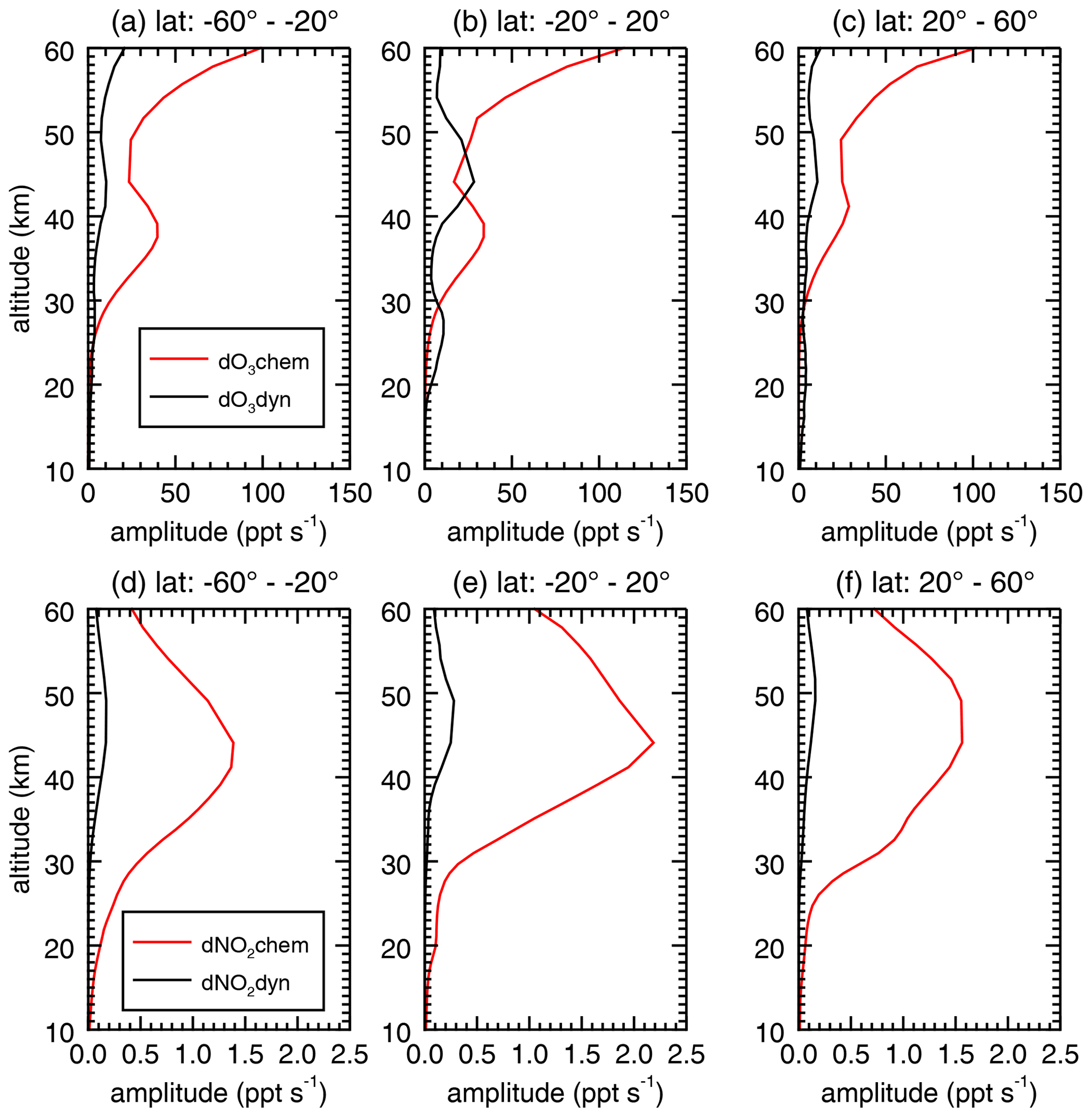
Figure 1The amplitude of the diurnal cycle of the simulated O3 tendency (a, b, c) and NO2 tendency (d, e, f) due to dynamics (black) and chemistry (red) for January 2019, averaged over three latitude bands.
We calculate scaling factors referenced to sunrise and sunset for easy application to SAGE III/ISS data when comparing to observations from different times of day. The factors are provided on an SZA by altitude grid with one file per month for January 2017 through December 2020. The SZA grid is nonlinear to allow finer resolution near the terminator when the values are changing rapidly. In addition to the year-specific scaling factors, we provide a monthly climatology of scaling factors, based on the average of 2017 through 2020, that can be applied to other time periods. We also provide the zonal mean concentrations of O3 and NO2 as functions of SZA, latitude, and altitude, so that users can derive their own scaling factors for arbitrary SZA pairs.
We compare the simulated NO2 and O3 profiles to observations from SAGE III/ISS and other instruments to determine the suitability and limitations of the simulated values for deriving scaling factors.
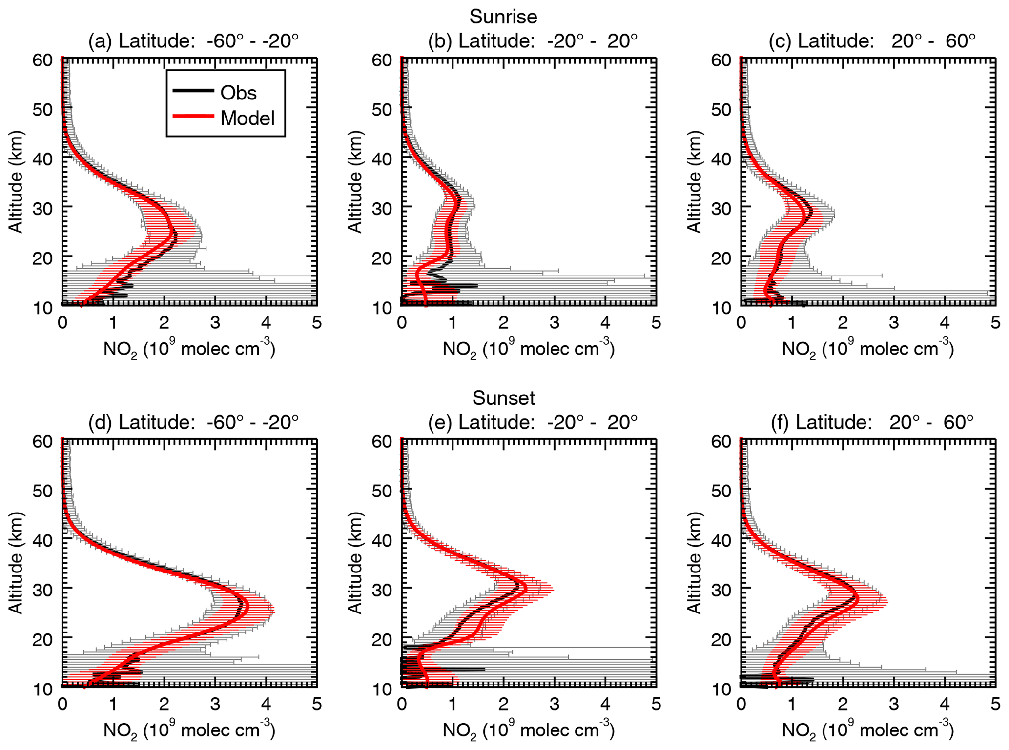
Figure 2Comparison of the model simulation (red) to SAGE III/ISS (black) sunrise (a, b, c) and sunset (d, e, f) NO2 vertical profile observations for December–January–February of 2017–2020 averaged over three different latitude bands. Error bars represent the standard deviation within the latitude band.
3.1 Comparison to NO2 observations
We compare the NO2 from our model simulation to sunrise and sunset observations from SAGE III/ISS. We note that the SZA diagnosed by the simulation sometimes deviates from that of the SAGE III/ISS observations at the same location, which by definition is ± 90∘ (depending on sunrise or sunset) and is reported for each event at the average longitude/latitude/time of all scans through a particular altitude. A mismatch in SZA can lead to disagreement between the simulated and observed NO2. Consequently, we sample the model by first determining the grid box corresponding to the SAGE III/ISS observation and then finding the grid box whose SZA best matches the SAGE III/ISS SZA (± 90∘) at the observation latitude within eight grid boxes (approximately 800 km) longitudinally of the observation location. This sampling methodology improves the agreement between the simulated and observed NO2.
Figure 2 shows the vertical profiles of simulated NO2 compared to SAGE III/ISS observations for sunrise and sunset for December through February of 2017–2020. Overall, the model simulation reproduces the major features of the vertical distribution and latitudinal variations of the SAGE III/ISS observations. The mean values are in good agreement at many altitudes and latitudes, but the simulation underestimates the SAGE III/ISS sunrise observations in the troposphere. Dubé et al. (2021) found that SAGE III/ISS NO2 is biased high, particularly at lower altitudes, and that accounting for diurnal variability along the line of sight can reduce the bias below 30 km by over 10 %. The sunset comparison shows a model overestimate at 20–30 km in the tropics. Between 20 and 40 km, the simulated profiles agree with the observed values within 20 %, except for the sunset profiles of the 20∘ S–20∘ N band, where the model overestimate reaches 40% at 20.5 km. However, comparison of the sunrise and sunset profiles suggests that the simulation is able to capture many of the observed sunrise–sunset differences. Figure S1 in the Supplement shows the sunrise and sunset NO2 comparisons for June–August of 2017–2020. There is good overall agreement between the simulated and observed NO2 in terms of the mean values and the profile shapes as well as how the profiles change between sunrise and sunset. The simulation underestimates the SAGE III/ISS peak around 30 km and places it slightly too low in the Southern Hemisphere. Both the simulation and the observations show lower values around 30 km for sunrise compared to sunset, consistent with the box model results of Dubé et al. (2020), since NOx concentrations increase over the day due to photolysis of N2O5 and other reservoir species (Belmonte Rivas et al., 2014). Increases in the NO2 column over the day are also seen in FTIR observations (Sussmann et al., 2005).
We also compare the simulated NO2 profiles to observations from the OSIRIS instrument (Llewellyn et al., 2004; Sioris et al., 2017). Figure S2 shows the comparison for July and August of 2017–2018. The simulation is biased high compared to OSIRIS throughout much of the profile between 10 and 40 km. The low biases seen in the SAGE III/ISS comparison (Fig. S1) are not present in the OSIRIS comparison. Some of this discrepancy may be due to the diurnal differences in NO2 along the line of sight (LOS) (Brohede et al., 2007; Dubé et al., 2021) that are not accounted for in the SAGE III/ISS retrieval.
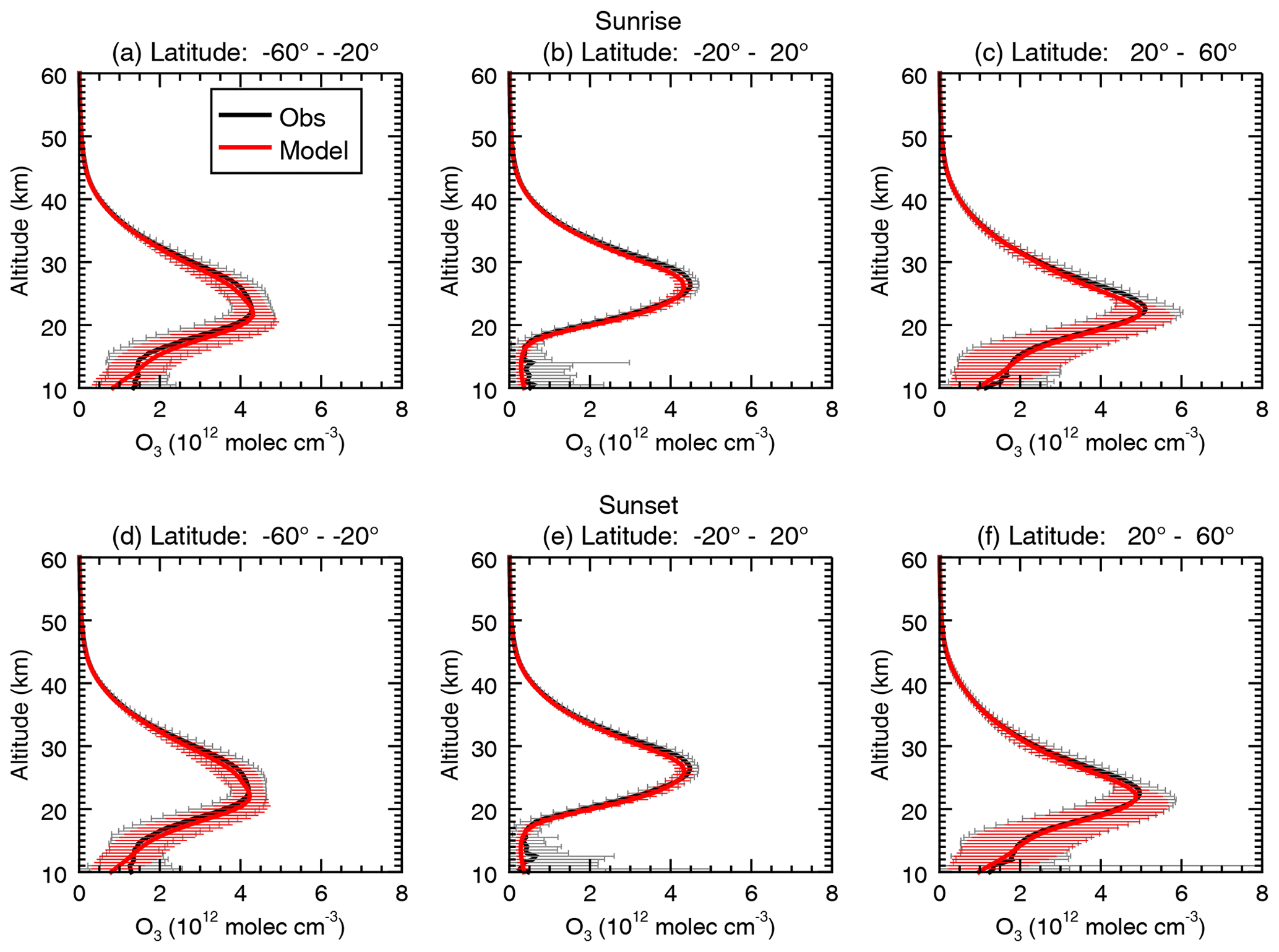
Figure 3Comparison of the model simulation (red) to SAGE III/ISS (black) sunrise (a, b, c) and sunset (d, e, f) O3 vertical profile observations for December–January–February of 2017–2020 averaged over three different latitude bands. Error bars represent the standard deviation within the latitude band.
3.2 Comparison to O3 observations
Previous studies have evaluated the stratospheric O3 and its variability in the GEOS model with GMI chemistry. Parrish et al. (2014) found reasonable agreement between the simulated O3 diurnal cycle at Mauna Loa, Hawaii, with microwave ozone profiling radiometer (MWR) observations at most levels, with most of the modeled and measured values agreeing to within 1.5 % of the midnight value. However, between 39 and 43 km, the morning vs. night differences in the MWR observations are 2 %–3 % higher than in the model. In addition, the diurnal peak relative to midnight is overestimated in the model compared to the MWR observations for 35–39 km in June–August. Frith et al. (2020) compared the climatological diurnal O3 cycle from a similar model simulation to the one in this paper to observations from the Superconducting Submillimeter-Wave Limb Emission Sounder (SMILES) and the Upper Atmosphere Research Satellite (UARS) MLS, with good agreement. They also compared the simulated day vs. night O3 differences to Aura MLS observations and the sunrise vs. sunset differences to SAGE III/ISS observations. They found good overall agreement with the structure of the MLS differences, generally within 2 %, while the simulated sunrise / sunset ratio differed from that of SAGE III/ISS above approximately 2 hPa but agreed within approximately a percent below 2 hPa.
We present additional validation of the simulated O3 with comparisons to SAGE III/ISS observations and ozonesondes. Figure 3 compares the simulated O3 with SAGE III/ISS observations from December–January–February of 2017–2020 for sunrise and sunset. There is good agreement between the model and observations above approximately 15 km. The model tends to underestimate the observations below 15 km, although the observations show large variability. Between 20 and 50 km, the model profiles for all three bands are within 15 % of the observations. The largest percent difference in this range for the sunrise observations is 13 % and occurs at 20 km for the 20∘ S–20∘ N band. The largest percent difference in this range for the sunset observations is 12 % and occurs at 20.5 km for the 20∘ S–20∘ N band. The model underestimates the O3 peak between approximately 25 and 30 km for the 20∘ S–20∘ N range. The SAGE III/ISS sunrise and sunset averages for this latitude band reach a peak of 4.5×10¹² molec cm−3 at 26.5 km, while the model reaches a peak of 4.3×10¹² molec cm−3 at 26 km. Similar features are seen in the June–August comparison (not shown) along with a small model overestimate around 15–20 km. For June–August, the model agrees with the observations within 30 % between 20 and 50 km, with the largest percent difference occurring at 20 km. Figure S3 shows a comparison of simulated O3 to ozonesonde profiles in three latitude ranges. There is good agreement in the profile shapes and latitudinal differences, but the simulated O3 is biased high in the 15–20 km range. Stauffer et al. (2019) also found a high bias in this region and attributed it partly to the model's limited vertical resolution causing discrepancies in the altitude of the tropopause gradient compared to sondes. The high bias below 10 km seen in the SAGE III/ISS comparison is not present in the ozonesonde comparison.
4.1 Diurnal scaling factors for NO2
In this section we describe the overall shape of the diurnal scaling factors for NO2 as well as their geographic and temporal variability. We then illustrate how application of the diurnal scale factors improves the agreement between observations taken at different times of day.
4.1.1 Description of NO2 diurnal scale factors
We present the climatological scale factors as a function of latitude, altitude, SZA, and month. Figure 4 shows the climatological sunrise and sunset diurnal scale factors for NO2 as a function of signed solar zenith angle for January and July at 45∘ N at 35 km. The U shape of the scaling factors reflects the high NO2 values at night and low values during the day, with sharp gradients occurring at sunrise (SZA = 90∘) and sunset (SZA = −90∘). The sunrise and sunset factors have a similar shape but are offset in magnitude because the sunrise and sunset values of NO2 differ as described in Sect. 3.1. Gaps in the plot represent SZA values that do not occur in the monthly mean. A larger gap around SZA = 0∘ occurs in January compared to July at 45∘ N, reflecting the lower Sun angle in January. The January scaling factors also reach a larger maximum value at night compared to the July factors at this latitude. While the overall shape of the NO2 scaling factors is similar across the altitude range of the SAGE III/ISS measurements, the magnitude changes dramatically with altitude because of the larger diurnal cycle of NO2 at higher altitudes. Figure S4 uses a nonlinear color scale to show the large amplitude of the diurnal scaling factors at high altitudes.
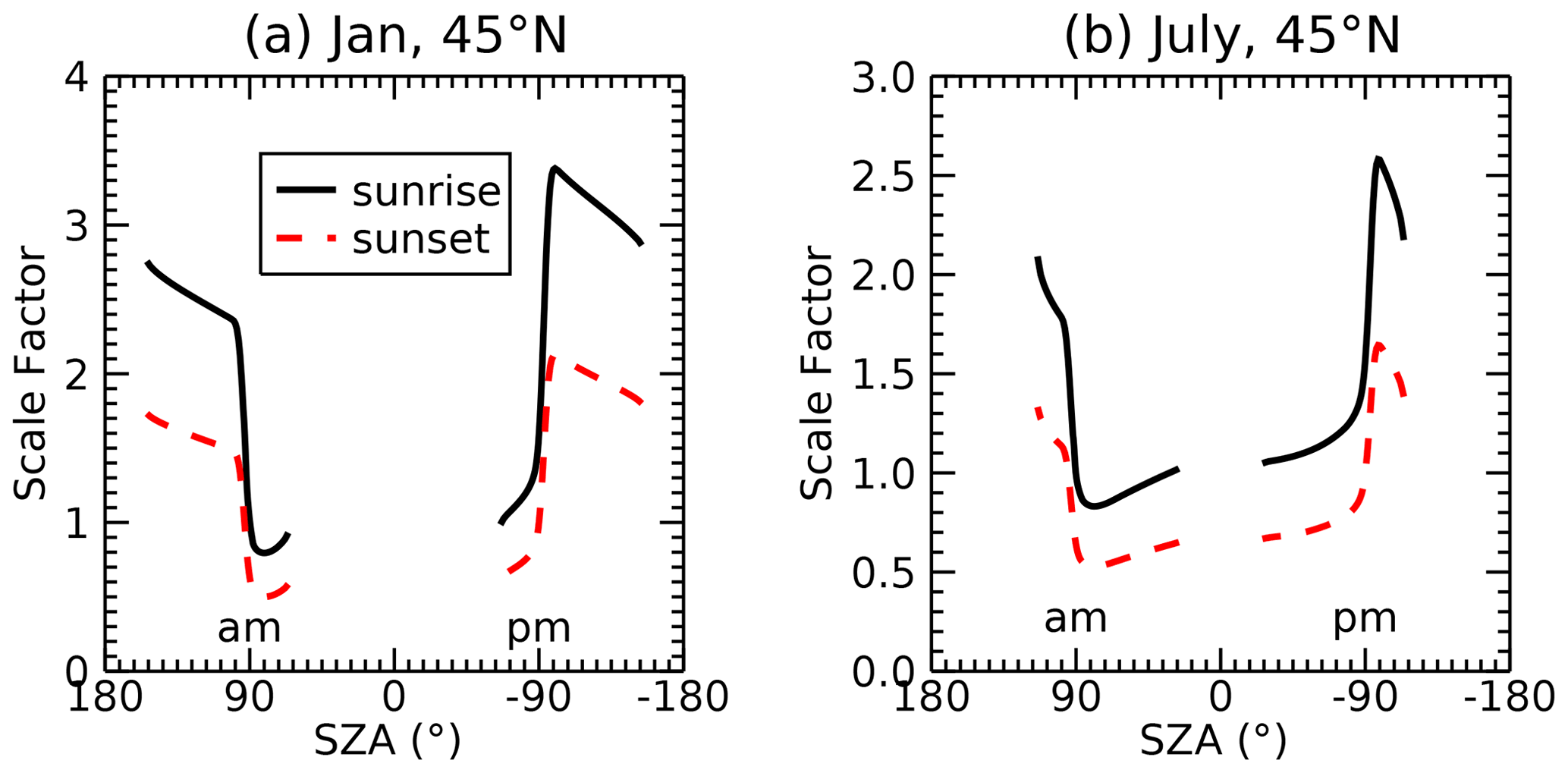
Figure 4Diurnal scaling factors for sunrise (black) and sunset (red) as a function of SZA at 45∘ N for (a) January and (b) July at 35 km altitude. The scaling factors represent the ratio of the NO2 at the given SZA to the values at sunrise or sunset.
We next explore the latitudinal variability in scaling factors using the sunrise factor for SZA = 60∘ at 35 km altitude as an example. We show the variations in the scale factor as a function of latitude for 1 month in each season in Fig. 5. There is considerable variability in the factor with both latitude and month. January shows the greatest variability, with values ranging from 0.65 at 69∘ S to 0.95 at 39∘ N. Both January and October show the largest deviation from 1 at the southern end of the range for which SZA = 60∘ is reached, while April and July deviate most strongly from 1 at the northern end.
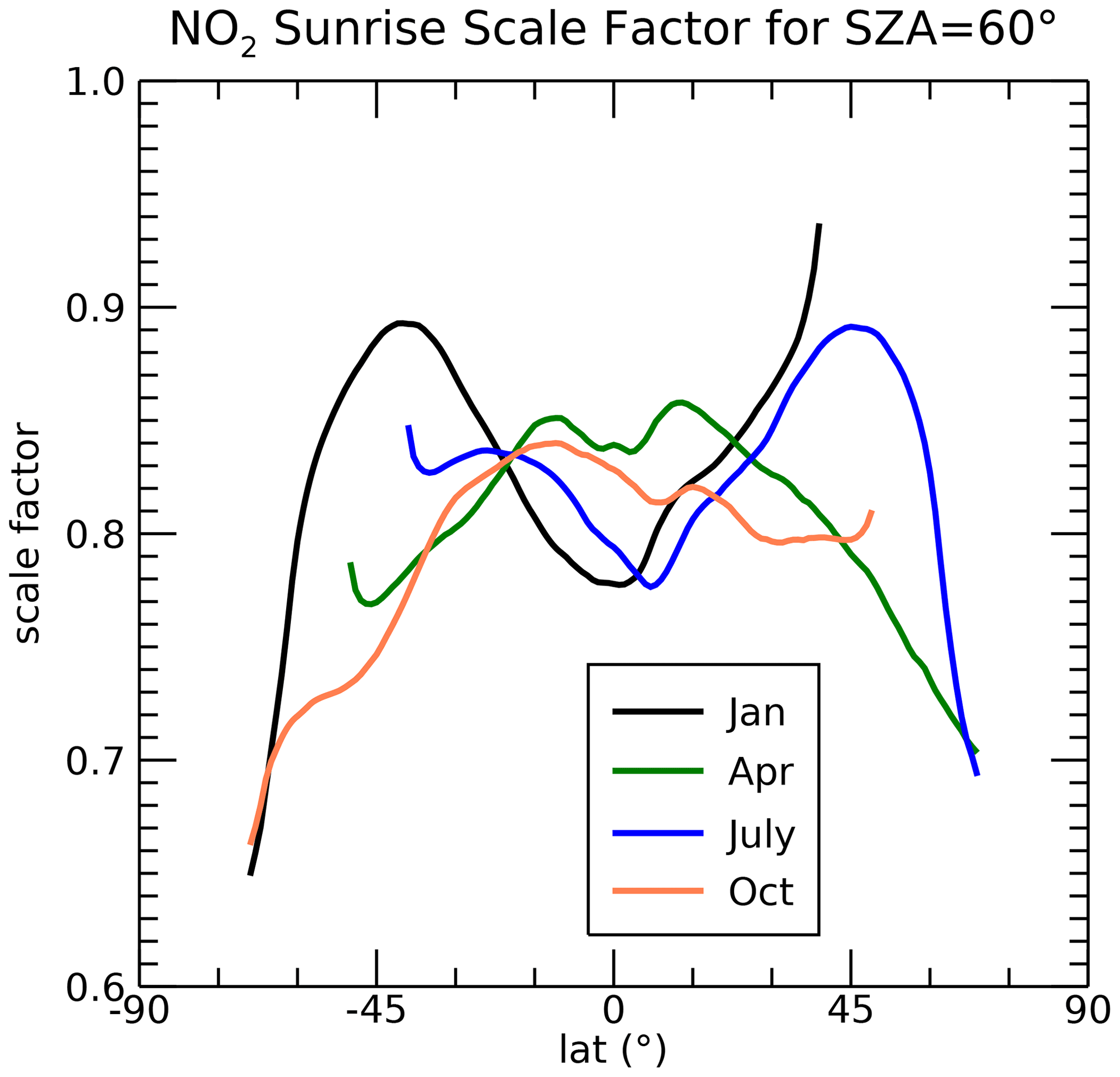
Figure 5The NO2 sunrise scale factor at 35 km for SZA = 60∘ as a function of latitude for January (black), April (green), July (blue), and October (orange).

Figure 6Interannual variability in the October sunrise NO2 scaling factors, which are referenced to SZA = 90∘. (a) Scaling factors as a function of signed SZA for the Equator at 25 km for the climatology (black), 2017 (orange), 2018 (magenta), 2019 (cyan), and 2020 (green). (b) Percent difference from climatology in the sunrise scaling factors (denoted “sunrise scale diff” in the axis labels) for SZA = 60∘ as a function of latitude for each year. (c) Percent difference from the climatology for the SZA = 60∘ scale factors for each year as a function of altitude at the Equator. (d) Percent difference from the climatology for the SZA = 60∘ scale factors for each year as a function of altitude at 60∘ S. (e) Simulated zonal mean zonal wind speed at the Equator as a function of altitude. (f) The vertical gradient in the zonal wind speed.
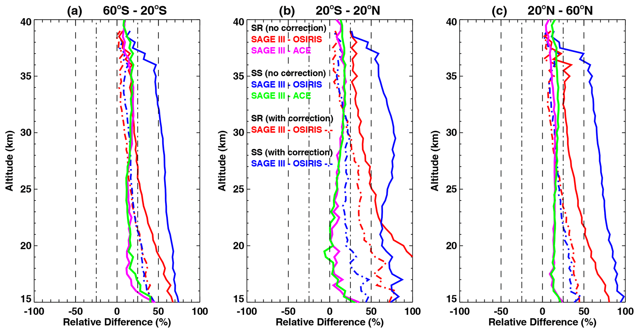
Figure 7The percent difference between SAGE III/ISS sunrise (SR) and sunset (SS) NO2 and OSIRIS and ACE-FTS observations averaged over three latitude bands. The OSIRIS comparisons without application of diurnal corrections are shown in solid red and blue lines for sunrise and sunset, respectively, while the comparisons with the diurnal scaling factors applied are shown in dashed red and blue lines for sunrise and sunset, respectively. The comparisons to ACE are shown in magenta for sunrise and green for sunset.
4.1.2 Interannual variability (IAV) of NO2 diurnal scale factors
Since we have created diurnal scale factors from both monthly climatological averages and from individual years, we investigate how much IAV exists in the NO2 diurnal scale factors. Figure 6 shows the IAV in the sunrise NO2 scaling factors for October. All 4 years show a similar shape for the factors as a function of signed SZA at the Equator at 25 km (Fig. 6a), but in 2018 the scale factors are larger than the climatology for SZA < 90∘, while for 2017 and 2019 they are smaller. The situation is reversed at the southern high latitudes, where 2018 and 2020 are smaller than the climatology and 2017 and 2019 are greater (Fig. 6b). Figure 6b shows that the percent difference between the individual years and the climatology is largest near the Equator and south of 60∘ S in October. Considering the difference from climatology for the SZA = 60∘ factor as a function of altitude, we find that, at the Equator, the differences are largest from approximately 15 to 35 km, but deviations from climatology do not exceed 15 % below 50 km (Fig. 6c). Park et al. (2017) found that the quasi-biennial oscillation (QBO) plays a dominant role in the IAV of tropical stratospheric NOx seen in OSIRIS observations. Zawodny and McCormick (1991) found that QBO variability of SAGE II NO2 was related to changes in the vertical transport of NOy and noted that the time of day could affect the relationship of NO2 with the QBO. We find that the yearly anomalies in the NO2 scale factors for the lower stratosphere show a similar vertical structure to the anomalies in the vertical gradient of the zonal wind anomalies at the Equator (Fig. 6f), indicating that variability associated with the QBO is likely responsible for the interannual variability at these altitudes.
At 60∘ S, the differences between individual years and climatology reach values above 20 % near 10–20 km (Fig. 6d). Considering all latitudes and altitudes below 50 km, the maximum difference between an individual year and climatology for the SZA = 60∘ factors is 54 % in October. The largest difference for the SZA = 60∘ factors when all months are considered is 75 %, which occurs in September at 23.5 km. When all SZA values between −90 and 90∘ are considered, the maximum difference reaches 118 % at 13.5 km in September. However, the IAV differs according to the month and latitude considered, so many of the differences average out when an entire year or large latitude range is considered.
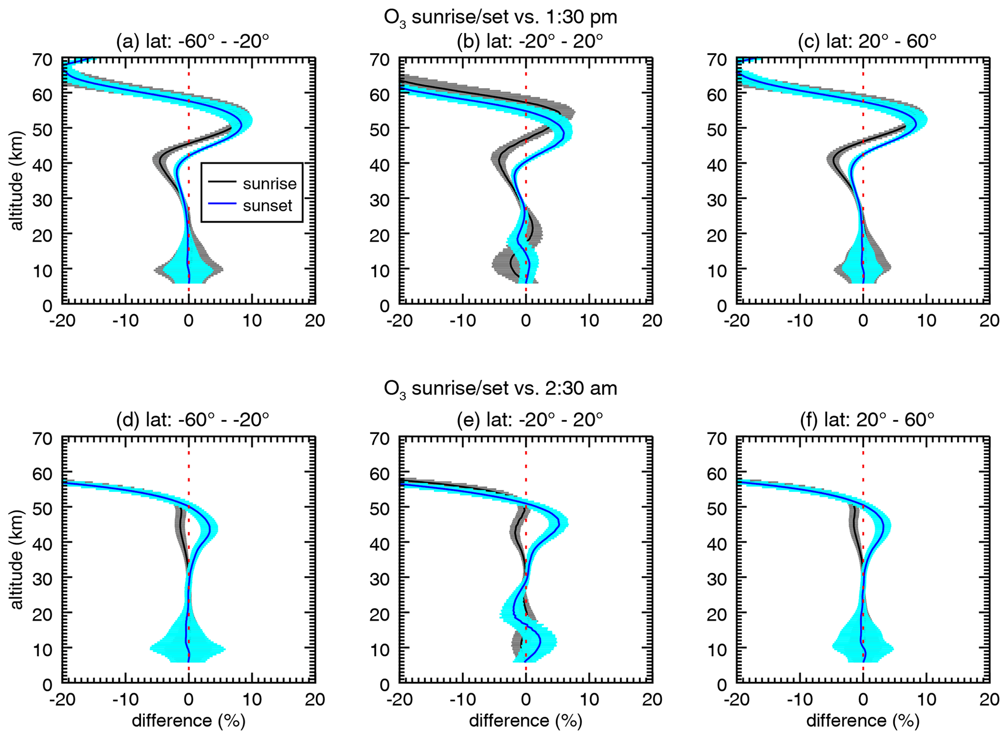
Figure 8The simulated percent difference in O3 between sunrise (black) or sunset (blue) vs. (a–c) 13:30 or (d–f) 02:30 for three latitude bands for all months of 2019. Error bars represent the variability within the band.

Figure 9Sunrise scale factors for O3 at 35 km as a function of SZA for January (solid lines) and July (dashed lines) at the Equator (black) and 60∘ S (red).
4.1.3 Application of NO2 diurnal scale factors
We demonstrate the utility of the NO2 diurnal scaling factors by comparing SAGE III/ISS NO2 observations with observations from OSIRIS with and without the application of the diurnal scaling factors. We also include the solar occultation ACE-FTS as a reference since it does not require any diurnal corrections when comparing with SAGE III/ISS. We note that the scale factors are intended to account for the temporal change in concentration between different observation times and not to alter the value of the SAGE III/ISS retrieval itself.
Figure 7 shows the percent difference between SAGE III/ISS sunrise (SR) and sunset (SS) and OSIRIS and ACE-FTS NO2 observations averaged over three latitude bands before and after applying the diurnal scale factors. The coincidence criteria between SAGE III and the reference instrument are defined as same-day measurements that are within 3∘ latitude and 10∘ longitude. For ACE-FTS, we matched SR/SS that met the criteria and were within 3 h of each other. In general, the disagreement between SAGE III and ACE-FTS for both sunrise and sunset measurements (magenta and green lines in Fig. 7) is 20 % or less for most altitudes. The difference between SAGE III and OSIRIS (red and blue solid lines) is large. The difference for sunrise observations exceeds 50 % below 20 km and exceeds 25 % below 35 km north of 20∘ S. Differences are especially large in the tropics below 22 km. Sunset differences exceed 50 % throughout much of the atmosphere below 35 km. NO2 diurnal variability and the mismatch of the measurement times explain much of these differences. The difference between the two instruments is significantly reduced when accounting for the NO2 diurnal cycle (red and blue dashed lines). The difference becomes mostly less than 50 % for both sunrise and sunset and below 25 % above 25 km, except for the sunrise observations between 20∘ S and 20∘ N. Applying the scaling factors improves the agreement between the SAGE and OSIRIS profiles in all latitude bands (Fig. 7) and improves the consistency between the sunrise and sunset comparisons, particularly in the 20–60∘ N and S ranges. The larger difference below 25 km is mostly caused by the diurnal effect error which occurs due to the variation of the SZA along the line of sight in occultation measurement. Like SAGE III, ACE-FTS does not account for the NO2 diurnal variability along the line of sight, and these two versions have a relatively uniform difference for all altitudes. The diurnal effect error is similar to what Brohede et al. (2007) found when comparing SAGE II and III to OSIRIS. In a recent study by Dubé et al. (2021), they attempted to correct for this effect in SAGE III/ISS NO2 measurements, which improved the agreement between SAGE III and OSIRIS below 20 km. However, they also noted that the corrections were not sufficient to account for all the differences at these altitudes.
The scale factors applied in this comparison were derived using individual months/years of the simulation. We found little difference when using monthly climatological scale factors, except for the year 2019 at altitudes between 10 and 20 km in the tropics and Northern Hemisphere (NH) midlatitude, where the difference can reach 2 % in the tropics and 7 % in the NH (not shown). It is therefore our recommendation that it is sufficient to use the global climatology when correcting for the NO2 diurnal variation in validation studies. However, we recommend using the month/year scale factor when merging multiple datasets for trend studies as differences caused by the QBO variability can be as large as 7 % below 20 km. Scale factors for specific years are also valuable when focusing on a specific month and region.
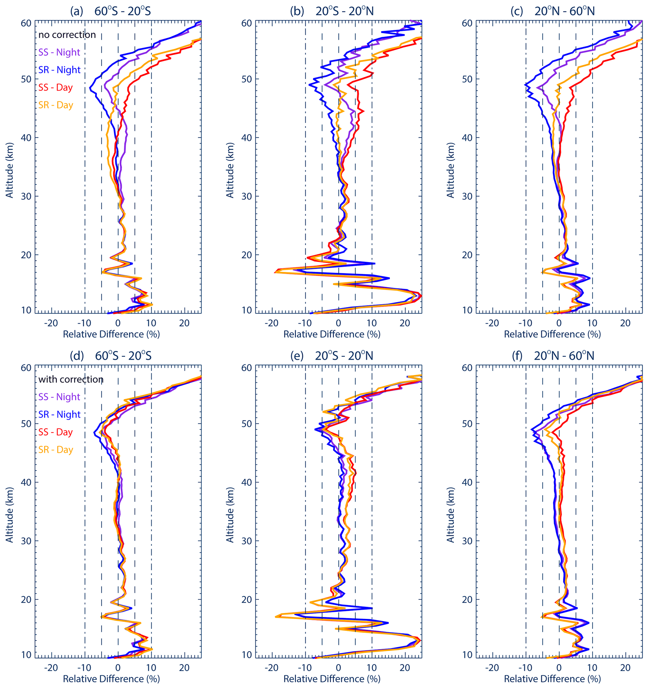
Figure 10(a, b, c) Comparison of SAGE III/ISS sunrise (red) and sunset (yellow) O3 observations with MLS daytime observations. Sunset and sunrise SAGE III/ISS observations are compared with MLS nighttime observations (purple and blue lines, respectively) in three different latitude zones. The relative difference is SAGE III − MLS and is shown in percent. No diurnal corrections are applied in this comparison. (d, e, f) Same as the top row but with the diurnal scaling factors applied.
4.2 Diurnal scaling factors for O3
This section presents the diurnal scaling factors for O3, including their temporal and spatial variability. We illustrate the importance of the diurnal correction for O3 in Fig. 8, which shows the difference between the simulated O3 at sunrise and sunset and the simulated O3 at 13:30, which is the approximate time of the MLS daytime overpass, and 02:30, corresponding to the MLS nighttime overpass. This difference represents the expected impact of the diurnal variability when comparing SAGE III/ISS observations with MLS daytime observations. Below approximately 25 km, the differences within latitude bands are small compared to the variability within the bands shown by the error bars. However, the average differences can also exceed 2% below 25 km in the tropics. The differences compared to MLS daytime observations increase above 25 km, although they remain within ±10 % until approximately 60 km (Fig. 8a–c). The sign of the difference switches between positive and negative depending on altitude. The sunrise O3 falls within a few percent of the MLS nighttime values for altitudes below 50 km, while somewhat larger relative differences are present for the sunset O3 between 35 and 50 km (Fig. 8d–f).
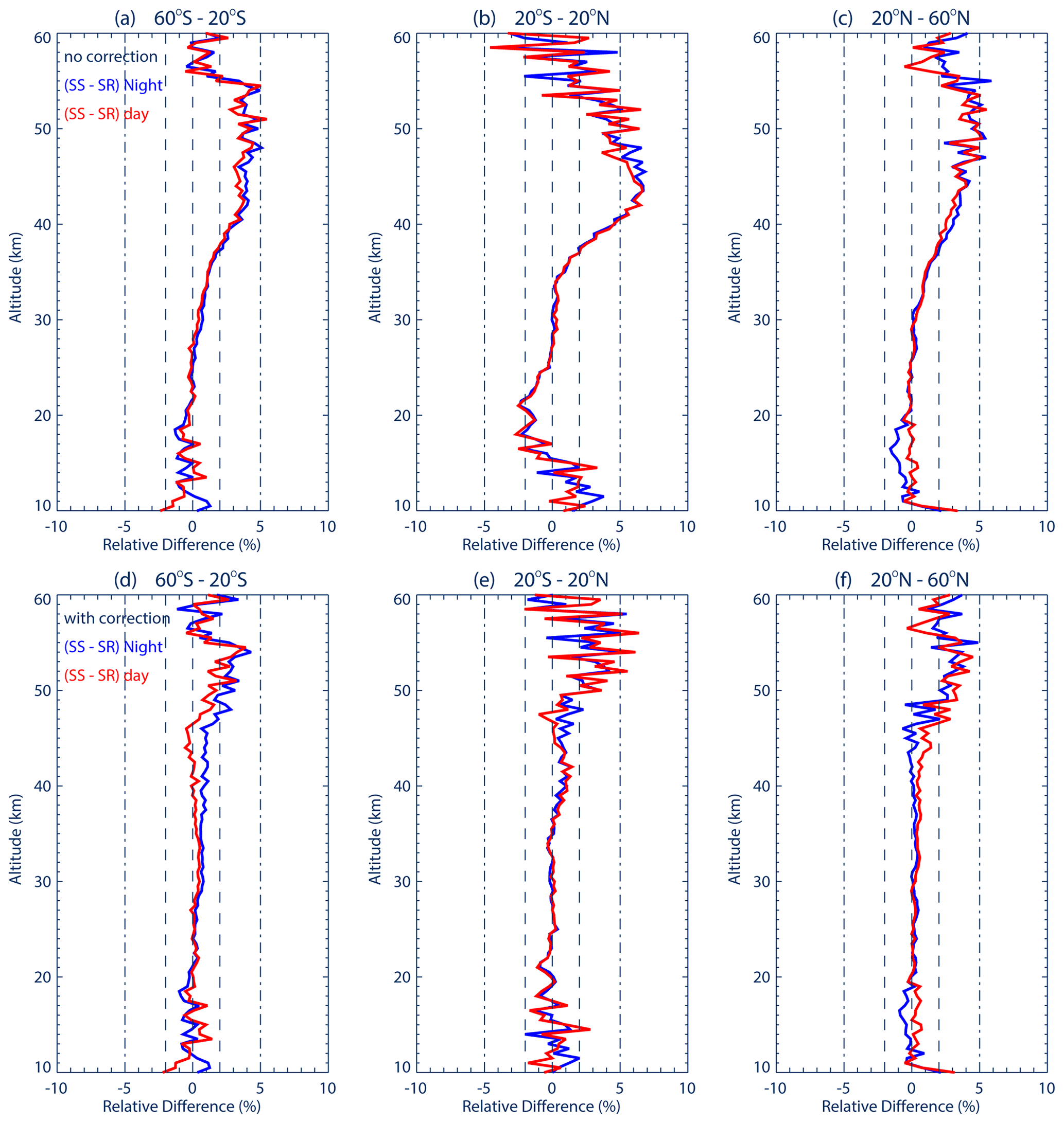
Figure 11(a, b, c) The difference (%) between SAGE III/ISS sunset (SS) and sunrise (SR) O3 observations in three different latitude zones when MLS daytime (red) and nighttime (blue) observations are used as a transfer standard. No diurnal corrections are applied in this comparison. (d, e, f) Same as the top row but with the diurnal scaling factors applied.
Figure 9 shows the shape of the sunrise diurnal scale factors for O3 at 35 km. We note that the y-axis range of Fig. 9 covers a smaller range of values than that of Fig. 4, which showed NO2 scale factors. The shape of the O3 scale factors at the Equator is similar for January and July (Fig. 9). Values dip shortly after sunrise (SZA = 90∘), rise over the course of the day to an afternoon peak, and then decrease until sunset. There is relatively little change in the nighttime (|SZA|> 90∘). This shape is even more pronounced at 60∘ S in January. The stronger variability at 60∘ S in Southern Hemisphere summer is consistent with the results of Schanz et al. (2014). The daytime increase to an afternoon maximum is consistent with the results of Haefele et al. (2008) and Parrish et al. (2014). Haefele et al. (2008) point out that production of odd oxygen by photolysis can explain this increase, since Ox is primarily O3 at this altitude. The dip after sunrise is consistent with the findings of Pallister and Tuck (1983), who attribute it to the photodissociation of NO2, followed by reaction of O3 with NO. The interannual variability in the O3 diurnal cycle diminishes below approximately 50 km (Fig. S5).
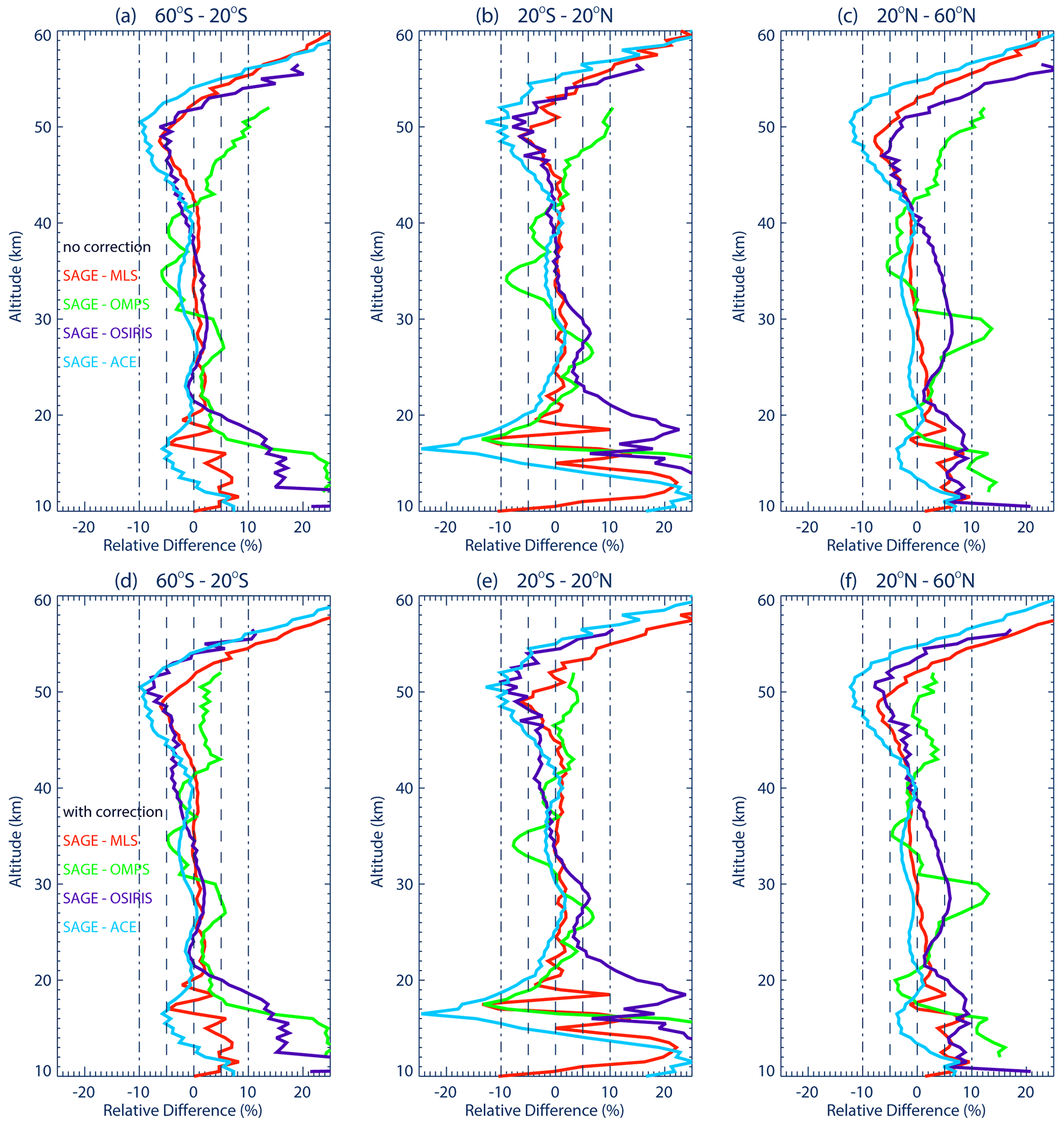
Figure 12(a, b, c) Comparison of SAGE III/ISS O3 observations with MLS nighttime observations (red), OMPS LP (green), OSIRIS (violet), and ACE-FTS (blue) in three different latitudinal zones. The relative difference is SAGE − instrument and is shown in percent. No diurnal corrections are applied in this comparison. (d, e, f) Same as the top row but with the diurnal scaling factors applied.
4.3 Application of O3 diurnal scale factors
To illustrate the utility of the derived O3 scaling factors, we compare SAGE III and MLS at different times with and without the diurnal corrections. The coincidence criteria used for all comparisons shown here are similar to those described in Sect. 4.1.2. MLS profiles were converted to number density and geometric altitude using MLS geopotential altitude, pressure, and temperature profiles. Figure 10 (top row) shows a comparison between SAGE III/ISS O3 observations at sunrise and sunset with daytime and nighttime MLS observations with no corrections for the diurnal cycle applied. The comparisons between the different time-of-day pairs diverge above approximately 35 km and exceed 10 % for the comparisons to MLS daytime observations above approximately 50 km. In addition, the sign of the difference between SAGE III/ISS observations and MLS observations is positive above 50 km, although the switch to positive occurs a few kilometers higher for the sunrise SAGE III/ISS vs. nighttime MLS cases. The bottom row of Fig. 10 shows the same comparison but with the diurnal scaling factors applied to account for differences due to the diurnal cycle. The spread between the different time-of-day pairings is greatly reduced above 35 km, providing a more consistent picture of the SAGE III/ISS vs. MLS O3 differences. In general, the difference between SAGE III/ISS and MLS is less than 5 % between 20 and 45 km. Application of the diurnal scaling factors reveals a consistent high bias in the SAGE III/ISS observations compared to MLS above 50 km.
Wang et al. (2020) reported a larger than expected diurnal magnitude of 5 %–8 % difference between SAGE III/ISS sunset and sunrise measurements in the upper stratosphere that they could not explain. We evaluate the differences in SAGE III/ISS sunrise vs. sunset measurements by comparing how they differ from MLS, similarly to Wang et al. (2020), who also used MLS observations as a transfer standard. Figure 11 shows the difference between SAGE III sunset and sunrise O3 observations using MLS daytime (blue) and nighttime (red) observations before and after applying the scale factors. The figure shows a 5 %–7 % difference at altitudes between 40 and 50 km, similar to the sunrise versus sunset differences shown in Fig. 7 by Wang et al. (2020). However, the difference is reduced significantly to less than 2 % through most of the 40–50 km range when applying the scale factors. Sunrise versus sunset differences are almost indistinguishable when using MLS daytime or nighttime measurements.
We also compared SAGE III to various satellite observations. Figure 12 shows the percent difference between SAGE III and MLS (night), OMPS-LP, OSIRIS, and ACE-FTS before (top) and after (bottom) applying the diurnal scale factor corrections. OMPS-LP and OSIRIS are limb scattering instruments that measure the O3 profiles at different times during the day. The figure shows that the difference between SAGE and correlative measurements is mostly within 5 % between 20 and 40 km, with some exceptions. ACE-FTS has a larger bias above 45 km similar to Sheese et al. (2017) and Wang et al. (2020), while OMPS LP has an over 10 % positive bias between 25 and 30 km in the NH, similar to Wang et al. (2020) and Kramarova et al. (2018). Around 50 km, the differences increase to 10 % between SAGE III and OMPS LP and ACE-FTS, but the bias compared to OMPS LP is positive at 50 km, while the bias compared to ACE-FTS, OSIRIS, and MLS is negative (Fig. 12, top). This difference compared to OMPS LP is largely reduced to within 5 % above 35 km once the scale factors are applied (Fig. 12, bottom). This is consistent with the finding of Frith et al. (2020) that accounting for the diurnal cycle reduced the differences between SAGE III/ISS and OMPS LP observations. This comparison illustrates the importance of accounting for the diurnal cycle of O3 when comparing observations from different times of the day or when merging multiple instruments used for trend studies. Above 50 km, the SAGE III/ISS observations are biased high compared to ACE-FTS and OSIRIS as well as MLS, consistent with the results in Fig. 10. As shown in Fig. S5, the variability of the scale factors is very small below 50 km. It is therefore our recommendation that using global climatology is sufficient to accurately correct for the O3 diurnal variations.
We used the GEOS-GMI global atmospheric chemistry model simulation to develop diurnal scale factors for 2017–2020 to account for differences between SAGE III/ISS and other observations due to the diurnal cycles of NO2 and O3. These scale factors provide a straightforward method for comparing observations from different times of day as they provide the ratios of O3 and NO2 at each solar zenith angle to their values at sunrise and sunset based on the simulated diurnal variability and account for dynamically and chemically driven variability. Furthermore, merging of the SAGE-measured photochemically active species, such as NO2 and O3 (above 45 km), with other satellite measurements is inherently difficult because of their strong diurnal variations. The diurnal scale factors can be used to scale all measurements to the same time of day. We validate the model simulation against SAGE III/ISS v5.2 retrievals and other observations and find good overall agreement in the profile shapes of NO2 and O3.
The scale factors vary with altitude, latitude, and month and are available for individual years to account for interannual variability. We also provide a monthly climatology based on the 2017–2020 average, which can be used to compare observations outside the 2017–2020 range. Interannual variability in the diurnal cycle of NO2 in the lower stratosphere is linked to the QBO. Overall, however, the interannual variability in the diurnal scale factors is relatively small in the stratosphere, especially for O3, so climatological scale factors are likely sufficient for most applications. However, accounting for IAV might be necessary when merging different NO2 datasets that are used for trend studies at altitudes above 40 km.
We show that application of the diurnal scale factors for NO2 improves this agreement between SAGE III/ISS and OSIRIS NO2 observations and the consistency between the comparisons for sunrise and sunset observations. The comparison between SAGE III/ISS and MLS O3 shows large differences in the magnitude and sign of the disagreement depending on whether sunrise or sunset SAGE III/ISS observations and daytime or nighttime MLS observations are considered. Application of the diurnal scale factors removes much of this variability, providing a more consistent view of the SAGE III/ISS vs. MLS O3 differences. Diurnal corrections can also account for the significant and unexplained differences in SAGE III/ISS sunrise vs. sunset O3 measurements reported by Wang et al. (2020). The scaling factors used in this study are now available as a tool to facilitate comparison between observations from different times of day. SAGE III/ISS V5.2 O3 agrees well with correlative measurements, with differences well within 5 % between 20 and 50 km when corrected for diurnal variability. Similarly, the SAGE III/ISS V5.2 NO2 agreement with correlative measurements is mostly within 10 %. The larger difference between SAGE III and OSIRIS below 25 km is caused by the diurnal effect from the variation of the SZA and hence the NO2 along the line of sight, which is neglected in the SAGE III retrieval and requires further corrections (Dubé et al., 2021).
The diurnal scale factors described in this work are available at https://avdc.gsfc.nasa.gov/pub/data/project/GMI_SF/ (Strode, 2021). SAGE III/ISS data are available from https://doi.org/10.5067/ISS/SAGEIII/SOLAR_BINARY_L2-V5.2 (NASA/LARC/SD/ASDC, 2017). OSIRIS data are available from https://research-groups.usask.ca/osiris/data-products.php (Roth, 2022). OMPS-LP data are available from https://doi.org/10.5067/X1Q9VA07QDS7 (Deland, 2017). ACE-FTS data are available from https://doi.org/10.20383/102.0495 (Bernath et al., 2021). MLS data are available from https://disc.gsfc.nasa.gov/datacollection/ML2O3_NRT_005.html (last access: 5 October 2022, EOS MLS Science Team (2022), 2022).
The supplement related to this article is available online at: https://doi.org/10.5194/amt-15-6145-2022-supplement.
SAS, GT, LDO, and MS designed the study. SAS created the scaling factors. SAS and GT performed the analyses, and LDO performed the model simulation. RS provided the ozonesonde comparison. RD and DF contributed scientific discussion of the SAGE III/ISS observations and CES contributed scientific discussion of the OSIRIS observations. SAS and GT wrote the manuscript, and all the co-authors contributed comments and editing of the manuscript.
The contact author has declared that none of the authors has any competing interests.
Publisher's note: Copernicus Publications remains neutral with regard to jurisdictional claims in published maps and institutional affiliations.
The ACE mission is supported by the Canadian Space Agency. GEOS-GMI development is supported by the NASA Modeling, Analysis, and Prediction (MAP) program, and computing resources were provided by the NASA Center for Climate Simulation (NCCS). We thank the instrument teams that provided the SAGE III/ISS, MLS, OSIRIS, ACE-FTS, and OMPS LP data.
This research has been supported by the National Aeronautics and Space Administration (grant no. 80NSSC18K0711).
This paper was edited by Ralf Sussmann and reviewed by two anonymous referees.
Adams, C., Bourassa, A. E., Sofieva, V., Froidevaux, L., McLinden, C. A., Hubert, D., Lambert, J.-C., Sioris, C. E., and Degenstein, D. A.: Assessment of Odin-OSIRIS ozone measurements from 2001 to the present using MLS, GOMOS, and ozonesondes, Atmos. Meas. Tech., 7, 49–64, https://doi.org/10.5194/amt-7-49-2014, 2014.
Belmonte Rivas, M., Veefkind, P., Boersma, F., Levelt, P., Eskes, H., and Gille, J.: Intercomparison of daytime stratospheric NO2 satellite retrievals and model simulations, Atmos. Meas. Tech., 7, 2203–2225, https://doi.org/10.5194/amt-7-2203-2014, 2014.
Bernath, P.: The Atmospheric Chemistry Experiment (ACE), J. Quant. Spectrosc. Ra. Transf., 186, 3–16, https://doi.org/10.1016/j.jqsrt.2016.04.006, 2017.
Bernath, P., McElroy, C., Abrams, M., Boone, C., Butler, M., Camy-Peyret, C., Carleer, M., Clerbaux, C., Coheur, P., Colin, R., DeCola, P., DeMaziere, M., Drummond, J., Dufour, D., Evans, W., Fast, H., Fussen, D., Gilbert, K., Jennings, D., Llewellyn, E., Lowe, R., Mahieu, E., McConnell, J., McHugh, M., McLeod, S., Michaud, R., Midwinter, C., Nassar, R., Nichitiu, F., Nowlan, C., Rinsland, C., Rochon, Y., Rowlands, N., Semeniuk, K., Simon, P., Skelton, R., Sloan, J., Soucy, M., Strong, K., Tremblay, P., Turnbull, D., Walker, K., Walkty, I., Wardle, D., Wehrle, V., Zander, R., and Zou, J.: Atmospheric Chemistry Experiment (ACE): Mission overview, Geophys. Res. Lett., 32, L15S01, https://doi.org/10.1029/2005GL022386, 2005.
Bernath, P., Boone, C., Steffen, J., and Crouse, J.: Atmospheric Chemistry Experiment SciSat Level 2 Processed Data, v3.5 / v3.6, Federated Research Data Repository [data set], https://doi.org/10.20383/102.0495, 2021.
Bian, H. and Prather, M.: Fast-J2: Accurate simulation of stratospheric photolysis in global chemical models, J. Atmos. Chem., 41, 281–296, https://doi.org/10.1023/A:1014980619462, 2002.
Brohede, S., Haley, C., McLinden, C., Sioris, C., Murtagh, D., Petelina, S., Llewellyn, E., Bazureau, A., Goutail, F., Randall, C., Lumpe, J., Taha, G., Thomasson, L., and Gordley, L.: Validation of Odin/OSIRIS stratospheric NO2 profiles, J. Geophys. Res.-Atmos., 112, D07310, https://doi.org/10.1029/2006JD007586, 2007.
Chin, M., Ginoux, P., Kinne, S., Torres, O., Holben, B., Duncan, B., Martin, R., Logan, J., Higurashi, A., and Nakajima, T.: Tropospheric aerosol optical thickness from the GOCART model and comparisons with satellite and Sun photometer measurements, J. Atmos. Sci., 59, 461–483, https://doi.org/10.1175/1520-0469(2002)059<0461:TAOTFT>2.0.CO;2, 2002.
Cisewski, M., Zawodny, J., Gasbarre, J., Eckman, R., Topiwala, N., Rodriguez-Alvarez, O., Cheek, D., and Hall, S.: The Stratospheric Aerosol and Gas Experiment (SAGE III) on the International Space Station (ISS) Mission, in: Sensors, Systems, and Next-Generation Satellites XVIII, vol. 9241, p. 924107, International Society for Optics and Photonics, Amsterdam, the Netherlands, 2014.
Colarco, P., da Silva, A., Chin, M., and Diehl, T.: Online simulations of global aerosol distributions in the NASA GEOS-4 model and comparisons to satellite and ground-based aerosol optical depth, J. Geophys. Res.-Atmos., 115, D14207, https://doi.org/10.1029/2009JD012820, 2010.
Crutzen, P.: Role of NO and NO2 in the Chemistry of the Troposphere and Stratosphere, Annu. Rev. Earth Planet. Sci., 7, 443–472, https://doi.org/10.1146/annurev.ea.07.050179.002303, 1979.
Damadeo, R. P., Zawodny, J. M., Remsberg, E. E., and Walker, K. A.: The impact of nonuniform sampling on stratospheric ozone trends derived from occultation instruments, Atmos. Chem. Phys., 18, 535–554, https://doi.org/10.5194/acp-18-535-2018, 2018.
Damadeo, R. P., Zawodny, J. M., Thomason, L. W., and Iyer, N.: SAGE version 7.0 algorithm: application to SAGE II, Atmos. Meas. Tech., 6, 3539–3561, https://doi.org/10.5194/amt-6-3539-2013, 2013.
Deland, M.: OMPS-NPP L2 LP Ozone (O3) Vertical Profile swath daily 3slit V2.5, Greenbelt, MD, USA, Goddard Earth Sciences Data and Information Services Center (GES DISC) [data set], https://doi.org/10.5067/X1Q9VA07QDS7, 2017.
Dube, K., Randel, W., Bourassa, A., Zawada, D., McLinden, C., and Degenstein, D.: Trends and Variability in Stratospheric NOx Derived From Merged SAGE II and OSIRIS Satellite Observations, J. Geophys. Res.-Atmos., 125, e2019JD031798, https://doi.org/10.1029/2019JD031798, 2020.
Dubé, K., Bourassa, A., Zawada, D., Degenstein, D., Damadeo, R., Flittner, D., and Randel, W.: Accounting for the photochemical variation in stratospheric NO2 in the SAGE III/ISS solar occultation retrieval, Atmos. Meas. Tech., 14, 557–566, https://doi.org/10.5194/amt-14-557-2021, 2021.
Duncan, B. N., Strahan, S. E., Yoshida, Y., Steenrod, S. D., and Livesey, N.: Model study of the cross-tropopause transport of biomass burning pollution, Atmos. Chem. Phys., 7, 3713–3736, https://doi.org/10.5194/acp-7-3713-2007, 2007.
EOS MLS Science Team (2022): MLS/Aura Near-Real-Time L2 Ozone (O3) Mixing Ratio V005, Greenbelt, MD, USA, Goddard Earth Sciences Data and Information Services Center (GES DISC) [data set], https://disc.gsfc.nasa.gov/datacollection/ML2O3_NRT_005.html, last access: 5 October 2022.
Flynn, L. E., Seftor, C. J., Larsen, J. C., and Xu, P.: The ozone mapping and profiler suite, in: Earth science satellite remote sensing, edited by: Qu, J. J., Gao, W., Kafatos, M., Murphy, R. E., and Salomonson, V. V., (pp. 279–296), Berlin: Springer, https://doi.org/10.1007/978-3-540-37293-6_15, 2006.
Frith, S. M., Bhartia, P. K., Oman, L. D., Kramarova, N. A., McPeters, R. D., and Labow, G. J.: Model-based climatology of diurnal variability in stratospheric ozone as a data analysis tool, Atmos. Meas. Tech., 13, 2733–2749, https://doi.org/10.5194/amt-13-2733-2020, 2020.
Gelaro, R., McCarty, W., Suarez, M., Todling, R., Molod, A., Takacs, L., Randles, C., Darmenov, A., Bosilovich, M., Reichle, R., Wargan, K., Coy, L., Cullather, R., Draper, C., Akella, S., Buchard, V., Conaty, A., da Silva, A., Gu, W., Kim, G., Koster, R., Lucchesi, R., Merkova, D., Nielsen, J., Partyka, G., Pawson, S., Putman, W., Rienecker, M., Schubert, S., Sienkiewicz, M., and Zhao, B.: The Modern-Era Retrospective Analysis for Research and Applications, Version 2 (MERRA-2), J. Climate, 30, 5419–5454, https://doi.org/10.1175/JCLI-D-16-0758.1, 2017.
Haefele, A., Hocke, K., Kampfer, N., Keckhut, P., Marchand, M., Bekki, S., Morel, B., Egorova, T., and Rozanov, E.: Diurnal changes in middle atmospheric H2O and O3: Observations in the Alpine region and climate models, J. Geophys. Res.-Atmos., 113, D17303, https://doi.org/10.1029/2008JD009892, 2008.
Harris, N. R. P., Hassler, B., Tummon, F., Bodeker, G. E., Hubert, D., Petropavlovskikh, I., Steinbrecht, W., Anderson, J., Bhartia, P. K., Boone, C. D., Bourassa, A., Davis, S. M., Degenstein, D., Delcloo, A., Frith, S. M., Froidevaux, L., Godin-Beekmann, S., Jones, N., Kurylo, M. J., Kyrölä, E., Laine, M., Leblanc, S. T., Lambert, J.-C., Liley, B., Mahieu, E., Maycock, A., de Mazière, M., Parrish, A., Querel, R., Rosenlof, K. H., Roth, C., Sioris, C., Staehelin, J., Stolarski, R. S., Stübi, R., Tamminen, J., Vigouroux, C., Walker, K. A., Wang, H. J., Wild, J., and Zawodny, J. M.: Past changes in the vertical distribution of ozone – Part 3: Analysis and interpretation of trends, Atmos. Chem. Phys., 15, 9965–9982, https://doi.org/10.5194/acp-15-9965-2015, 2015.
Kerzenmacher, T., Wolff, M. A., Strong, K., Dupuy, E., Walker, K. A., Amekudzi, L. K., Batchelor, R. L., Bernath, P. F., Berthet, G., Blumenstock, T., Boone, C. D., Bramstedt, K., Brogniez, C., Brohede, S., Burrows, J. P., Catoire, V., Dodion, J., Drummond, J. R., Dufour, D. G., Funke, B., Fussen, D., Goutail, F., Griffith, D. W. T., Haley, C. S., Hendrick, F., Höpfner, M., Huret, N., Jones, N., Kar, J., Kramer, I., Llewellyn, E. J., López-Puertas, M., Manney, G., McElroy, C. T., McLinden, C. A., Melo, S., Mikuteit, S., Murtagh, D., Nichitiu, F., Notholt, J., Nowlan, C., Piccolo, C., Pommereau, J.-P., Randall, C., Raspollini, P., Ridolfi, M., Richter, A., Schneider, M., Schrems, O., Silicani, M., Stiller, G. P., Taylor, J., Tétard, C., Toohey, M., Vanhellemont, F., Warneke, T., Zawodny, J. M., and Zou, J.: Validation of NO2 and NO from the Atmospheric Chemistry Experiment (ACE), Atmos. Chem. Phys., 8, 5801–5841, https://doi.org/10.5194/acp-8-5801-2008, 2008.
Kramarova, N. A., Bhartia, P. K., Jaross, G., Moy, L., Xu, P., Chen, Z., DeLand, M., Froidevaux, L., Livesey, N., Degenstein, D., Bourassa, A., Walker, K. A., and Sheese, P.: Validation of ozone profile retrievals derived from the OMPS LP version 2.5 algorithm against correlative satellite measurements, Atmos. Meas. Tech., 11, 2837–2861, https://doi.org/10.5194/amt-11-2837-2018, 2018.
Livesey, N. J., Read, W. G., Wagner, P. A., Froidevaux, L., Lambert, A., Manney, G. L., Millán Valle, L. F., Pumphrey, H. C., Santee, M. L., Schwartz, M. J., Wang, S., Fuller, R. A., Jarnot, R. F., Knosp, B. W., Martinez, E., and Lay, R. R.: Earth Observing System (EOS) Aura Microwave Limb Sounder (MLS) Version 4.2x Level 2 and 3 data quality and description document, JPL D-33509 Rev. E, 2020.
Livesey, N. J., Read, W. G., Wagner, P. A., Froidevaux, L., Santee, M. L., Schwartz, M. J., Lambert, A., Millán Valle, L. F., Pumphrey, H. C., Manney, G. L., Fuller, R. A., Jarnot, R. F., Knosp, B. W., and Lay, R. R.: Earth Observing System (EOS) Aura Microwave Limb Sounder (MLS) Version 5.0x Level 2 and 3 data quality and description document, JPL D-105336 Rev. B, 2022.
Llewellyn, E., Lloyd, N., Degenstein, D., Gattinger, R., Petelina, S., Bourassa, A., Wiensz, J., Ivanov, E., McDade, I., Solheim, B., McConnell, J., Haley, C., von Savigny, C., Sioris, C., McLinden, C., Griffioen, E., Kaminski, J., Evans, W., Puckrin, E., Strong, K., Wehrle, V., Hum, R., Kendall, D., Matsushita, J., Murtagh, D., Brohede, S., Stegman, J., Witt, G., Barnes, G., Payne, W., Piche, L., Smith, K., Warshaw, G., Deslauniers, D., Marchand, P., Richardson, E., King, R., Wevers, I., McCreath, W., Kyrola, E., Oikarinen, L., Leppelmeier, G., Auvinen, H., Megie, G., Hauchecorne, A., Lefevre, F., de La Noe, J., Ricaud, P., Frisk, U., Sjoberg, F., von Scheele, F., and Nordh, L.: The OSIRIS instrument on the Odin spacecraft, Can. J. Phys., 82, 411–422, https://doi.org/10.1139/P04-005, 2004.
McCorimick, M., Zawodny, J., Veiga, R., Larsen, J., and Wang, P.: An Overview of SAGE-I and SAGE-II Ozone Measurements, Planet. Space Sci., 37, 1567–1586, https://doi.org/10.1016/0032-0633(89)90146-3, 1989.
McLinden, C., Haley, C., and Sioris, C.: Diurnal effects in limb scatter observations, J. Geophys. Res.-Atmos., 111, D14302, https://doi.org/10.1029/2005JD006628, 2006.
Molod, A., Takacs, L., Suarez, M., and Bacmeister, J.: Development of the GEOS-5 atmospheric general circulation model: evolution from MERRA to MERRA2, Geosci. Model Dev., 8, 1339–1356, https://doi.org/10.5194/gmd-8-1339-2015, 2015.
Murtagh, D., Frisk, U., Merino, F., Ridal, M., Jonsson, A., Stegman, J., Witt, G., Eriksson, P., Jimenez, C., Megie, G., de la Noe, J., Ricaud, P., Baron, P., Pardo, J., Hauchcorne, A., Llewellyn, E., Degenstein, D., Gattinger, R., Lloyd, N., Evans, W., McDade, I., Haley, C., Sioris, C., von Savigny, C., Solheim, B., McConnell, J., Strong, K., Richardson, E., Leppelmeier, G., Kyrola, E., Auvinen, H., and Oikarinen, L.: An overview of the Odin atmospheric mission, Can. J. Phys., 80, 309–319, https://doi.org/10.1139/P01-157, 2002.
NASA/LARC/SD/ASDC: SAGE III/ISS L2 Solar Event Species Profiles (Native) V052, ASDC [data set], https://doi.org/10.5067/ISS/SAGEIII/SOLAR_BINARY_L2-V5.2, 2017.
Nielsen, J., Pawson, S., Molod, A., Auer, B., da Silva, A., Douglass, A., Duncan, B., Liang, Q., Manyin, M., Oman, L., Putman, W., Strahan, S., and Wargan, K.: Chemical Mechanisms and Their Applications in the Goddard Earth Observing System (GEOS) Earth System Model, J. Adv. Model. Earth Syst., 9, 3019–3044, https://doi.org/10.1002/2017MS001011, 2017.
Orbe, C., Oman, L., Strahan, S., Waugh, D., Pawson, S., Takacs, L., and Molod, A.: Large-Scale Atmospheric Transport in GEOS Replay Simulations, J. Adv. Model. Earth Syst., 9, 2545–2560, https://doi.org/10.1002/2017MS001053, 2017.
Pallister, R. and Tuck, A.: The Diurnal-Variation of Ozone in the Upper-Stratosphere as a Test of Photochemical Theory, Q. J. Roy. Meteorol. Soc., 109, 271–284, https://doi.org/10.1002/qj.49710946002, 1983.
Park, M., Randel, W., Kinnison, D., Bourassa, A., Degenstein, D., Roth, C., McLinden, C., Sioris, C., Livesey, N., and Santee, M.: Variability of Stratospheric Reactive Nitrogen and Ozone Related to the QBO, J. Geophys. Res.-Atmos., 122, 10103–10118, https://doi.org/10.1002/2017JD027061, 2017.
Parrish, A., Boyd, I. S., Nedoluha, G. E., Bhartia, P. K., Frith, S. M., Kramarova, N. A., Connor, B. J., Bodeker, G. E., Froidevaux, L., Shiotani, M., and Sakazaki, T.: Diurnal variations of stratospheric ozone measured by ground-based microwave remote sensing at the Mauna Loa NDACC site: measurement validation and GEOSCCM model comparison, Atmos. Chem. Phys., 14, 7255–7272, https://doi.org/10.5194/acp-14-7255-2014, 2014.
Prather, M.: Ozone in the Upper-Stratosphere and Mesosphere, J. Geophys. Res.-Oceans, 86, 5325–5338, https://doi.org/10.1029/JC086iC06p05325, 1981.
Prather, M.: Catastrophic Loss of Stratospheric Ozone in Dense Volcanic Clouds, J. Geophys. Res.-Atmos., 97, 10187–10191, https://doi.org/10.1029/92JD00845, 1992.
Prather, M. and Jaffe, A.: Global Impact of the Antarctic Ozone Hole – Chemical-Propagation, J. Geophys. Res.-Atmos., 95, 3473–3492, https://doi.org/10.1029/JD095iD04p03473, 1990.
Roth, C.: OSIRIS on ODIN, University of Saskatchewan [data set], https://research-groups.usask.ca/osiris/data-products.php, last access: 7 October 2022.
SAGE III ATBD: SAGE III Algorithm Theoretical Basis Document: Solar and Lunar Algorithm, Earth Observing System Project science Office, https://eospso.gsfc.nasa.gov/sites/default/files/atbd/atbd-sage-solar-lunar.pdf (last access: 18 August 2021), 2002.
SAGE III/ISS V5.2 release notes, available at: https://asdc.larc.nasa.gov/project/SAGE III-ISS/g3bsspb_52, last access: 14 September 2021.
Sakazaki, T., Shiotani, M., Suzuki, M., Kinnison, D., Zawodny, J. M., McHugh, M., and Walker, K. A.: Sunset–sunrise difference in solar occultation ozone measurements (SAGE II, HALOE, and ACE–FTS) and its relationship to tidal vertical winds, Atmos. Chem. Phys., 15, 829–843, https://doi.org/10.5194/acp-15-829-2015, 2015.
Sakazaki, T., Fujiwara, M., Mitsuda, C., Imai, K., Manago, N., Naito, Y., Nakamura, T., Akiyoshi, H., Kinnison, D., Sano, T., Suzuki, M., and Shiotani, M.: Diurnal ozone variations in the stratosphere revealed in observations from the Superconducting Submillimeter-Wave Limb-Emission Sounder (SMILES) on board the International Space Station (ISS), J. Geophys. Res.-Atmos., 118, 2991–3006, https://doi.org/10.1002/jgrd.50220, 2013.
Schanz, A., Hocke, K., and Kämpfer, N.: Daily ozone cycle in the stratosphere: global, regional and seasonal behaviour modelled with the Whole Atmosphere Community Climate Model, Atmos. Chem. Phys., 14, 7645–7663, https://doi.org/10.5194/acp-14-7645-2014, 2014.
Schanz, A., Hocke, K., Kämpfer, N., Chabrillat, S., Inness, A., Palm, M., Notholt, J., Boyd, I., Parrish, A., and Kasai, Y.: The Diurnal Variation in Stratospheric Ozone from MACC Reanalysis, ERA-Interim,WACCM, and Earth Observation Data: Characteristics and Intercomparison, Atmosphere, 12, 625, https://doi.org/10.3390/atmos12050625, 2021.
Schoeberl, M. R., Douglass, A. R., Hilsenrath, E., Bhartia, P. K., Beer, R., Waters, J. W., Gunson, M. R., Froidevaux, L., Gille, J. C., Barnett, J. J., Levelt, P. E., and DeCola, P.: Overview of the EOS Aura Mission, IEEE Trans. Geosci. Remote Sens., 44, 1066–1074, https://doi.org/10.1109/tgrs.2005.861950, 2006.
Schoeberl, M., Jensen, E., Wang, T., Taha, G., Ueyama, R., Wang, Y., DeLand, M., and Dessler, A.: Cloud and aerosol distributions from SAGE III/ISS observations, J. Geophys. Res.-Atmos., 126, e2021JD035550, https://doi.org/10.1029/2021JD035550, 2021.
Sheese, P., Walker, K., Boone, C., Bernath, P., Froidevaux, L., Funke, B., Raspollini, P., and von Clarmann, T.: ACE-FTS ozone, water vapour, nitrous oxide, nitric acid, and carbon monoxide profile comparisons with MIPAS and MLS, J. Quant. Spectrosc. Ra. Transf., 186, 63–80, https://doi.org/10.1016/j.jqsrt.2016.06.026, 2017.
Sheese, P. E., Walker, K. A., Boone, C. D., Bourassa, A. E., Degenstein, D. A., Froidevaux, L., McElroy, C. T., Murtagh, D., Russell III, J. M., and Zou, J.: Assessment of the quality of ACE-FTS stratospheric ozone data, Atmos. Meas. Tech., 15, 1233–1249, https://doi.org/10.5194/amt-15-1233-2022, 2022.
Sioris, C. E., Rieger, L. A., Lloyd, N. D., Bourassa, A. E., Roth, C. Z., Degenstein, D. A., Camy-Peyret, C., Pfeilsticker, K., Berthet, G., Catoire, V., Goutail, F., Pommereau, J.-P., and McLinden, C. A.: Improved OSIRIS NO2 retrieval algorithm: description and validation, Atmos. Meas. Tech., 10, 1155–1168, https://doi.org/10.5194/amt-10-1155-2017, 2017.
Solomon, S., Russell, J., and Gordley, L.: Observations of the Diurnal-Variation of Nitrogen-Dioxide in the Stratosphere, J. Geophys. Res.-Atmos., 91, 5455–5464, https://doi.org/10.1029/JD091iD05p05455, 1986.
Stauffer, R., Thompson, A., Oman, L., and Strahan, S.: The Effects of a 1998 Observing System Change on MERRA-2-Based Ozone Profile Simulations, J. Geophys. Res.-Atmos., 124, 7429–7441, https://doi.org/10.1029/2019JD030257, 2019.
Strahan, S. E., Duncan, B. N., and Hoor, P.: Observationally derived transport diagnostics for the lowermost stratosphere and their application to the GMI chemistry and transport model, Atmos. Chem. Phys., 7, 2435–2445, https://doi.org/10.5194/acp-7-2435-2007, 2007.
Strode, S: Diurnal Scaling Factors, NASA [data set], https://avdc.gsfc.nasa.gov/pub/data/project/GMI_SF/ (last access: 7 October 2022), 2021.
Strode, S., Ziemke, J., Oman, L., Lamsal, L., Olsen, M., and Liu, J.: Global changes in the diurnal cycle of surface ozone, Atmos. Environ., 199, 323–333, https://doi.org/10.1016/j.atmosenv.2018.11.028, 2019.
Studer, S., Hocke, K., Schanz, A., Schmidt, H., and Kämpfer, N.: A climatology of the diurnal variations in stratospheric and mesospheric ozone over Bern, Switzerland, Atmos. Chem. Phys., 14, 5905–5919, https://doi.org/10.5194/acp-14-5905-2014, 2014.
Sussmann, R., Stremme, W., Burrows, J. P., Richter, A., Seiler, W., and Rettinger, M.: Stratospheric and tropospheric NO2 variability on the diurnal and annual scale: a combined retrieval from ENVISAT/SCIAMACHY and solar FTIR at the Permanent Ground-Truthing Facility Zugspitze/Garmisch, Atmos. Chem. Phys., 5, 2657–2677, https://doi.org/10.5194/acp-5-2657-2005, 2005.
Vaughan, G.: Diurnal-Variation of Mesospheric Ozone, Nature, 296, 133–135, https://doi.org/10.1038/296133a0, 1982.
Wang, H., Cunnold, D., Trepte, C., Thomason, L., and Zawodny, J.: SAGE III solar ozone measurements: Initial results, Geophys. Res. Lett., 33, L03805, https://doi.org/10.1029/2005GL025099, 2006.
Wang, H., Damadeo, R., Flittner, D., Kramarova, N., Taha, G., Davis, S., Thompson, A., Strahan, S., Wang, Y., Froidevaux, L., Degenstein, D., Bourassa, A., Steinbrecht, W., Walker, K., Querel, R., Leblanc, T., Godin-Beekmann, S., Hurst, D., and Hall, E.: Validation of SAGE III/ISS Solar Occultation Ozone Products With Correlative Satellite and Ground-Based Measurements, J. Geophys. Res.-Atmos., 125, e2020JD032430, https://doi.org/10.1029/2020JD032430, 2020.
Waters, J., Froidevaux, L., Harwood, R., Jarnot, R., Pickett, H., Read, W., Siegel, P., Cofield, R., Filipiak, M., Flower, D., Holden, J., Lau, G., Livesey, N., Manney, G., Pumphrey, H., Santee, M., Wu, D., Cuddy, D., Lay, R., Loo, M., Perun, V., Schwartz, M., Stek, P., Thurstans, R., Boyles, M., Chandra, K., Chavez, M., Chen, G., Chudasama, B., Dodge, R., Fuller, R., Girard, M., Jiang, J., Jiang, Y., Knosp, B., LaBelle, R., Lam, J., Lee, K., Miller, D., Oswald, J., Patel, N., Pukala, D., Quintero, O., Scaff, D., Van Snyder, W., Tope, M., Wagner, P., and Walch, M.: The Earth Observing System Microwave Limb Sounder (EOS MLS) on the Aura satellite, IEEE Trans. Geosci. Remote Sens., 44, 1075–1092, https://doi.org/10.1109/TGRS.2006.873771, 2006.
WMO (World Meteorological Organization): Report of the International Ozone Trends Panel 1988, Global Ozone Research and Monitoring Project-Report No. 18, World Meteorological Organization, Geneva, Switzerland, https://csl.noaa.gov/assessments/ozone/1988/report.html (last access: 18 October 2022), 1988.
WMO (World Meteorological Organization): Scientific Assessment of Ozone Depletion: 2010, Global Ozone Research and Monitoring Project-Report No. 52, 516 pp., Geneva, Switzerland, https://csl.noaa.gov/assessments/ozone/2010/report.html (last access: 18 October 2022), 2011.
Zawodny, J. M. and McCormick, M. P.: Stratospheric Aerosol and Gas Experiment II Measurements of the Quasi-Biennial Oscillations in Ozone and Nitrogen Dioxide, J. Geophys. Res.-Atmos., 96, 9371–9377, https://doi.org/10.1029/91JD00517, 1991.